
Antenna Arrangement in UWB Helmet Brain Applicators for Deep Microwave Hyperthermia


Abstract
:Simple Summary
Abstract
1. Introduction
2. Method
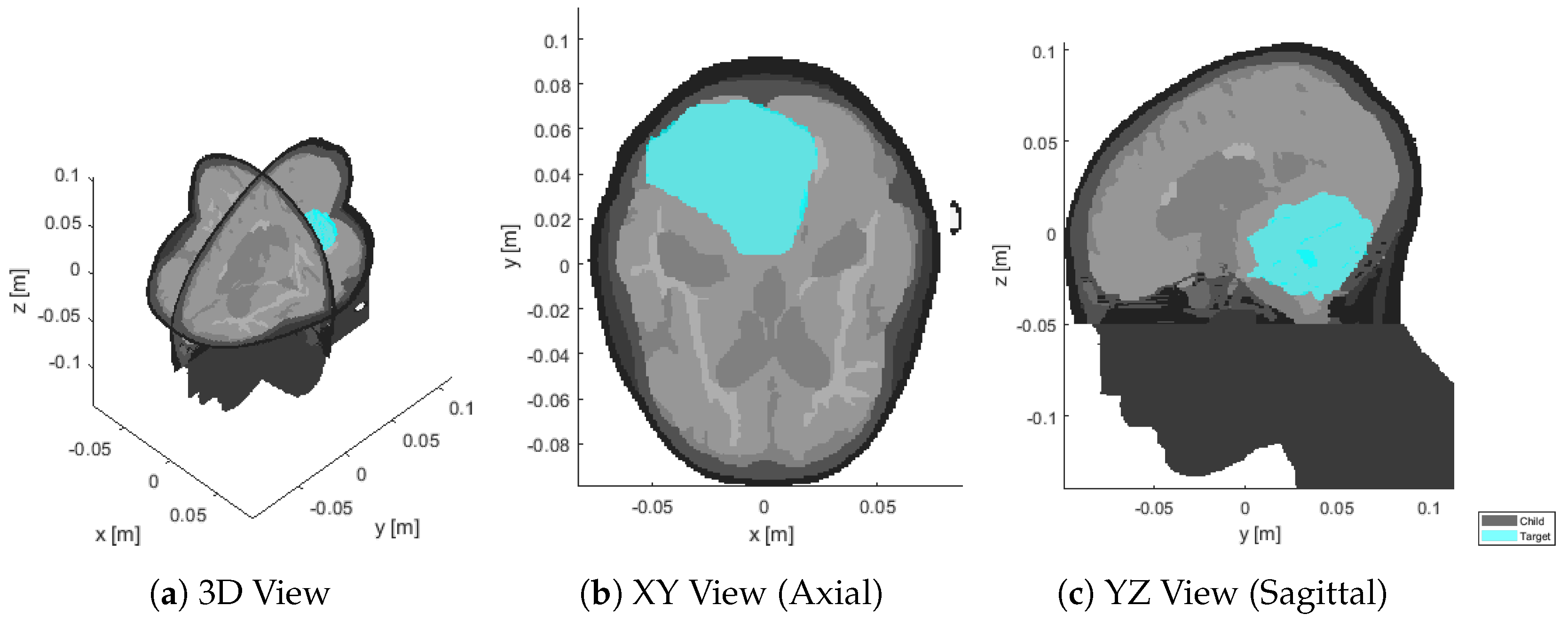
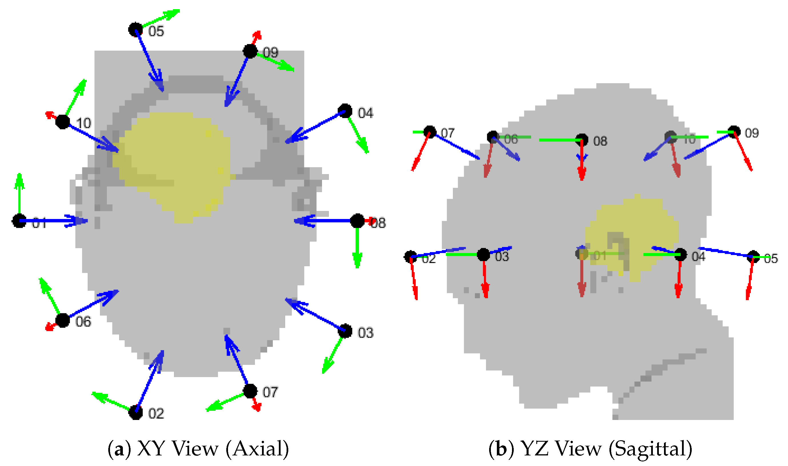
2.1. Patient Model
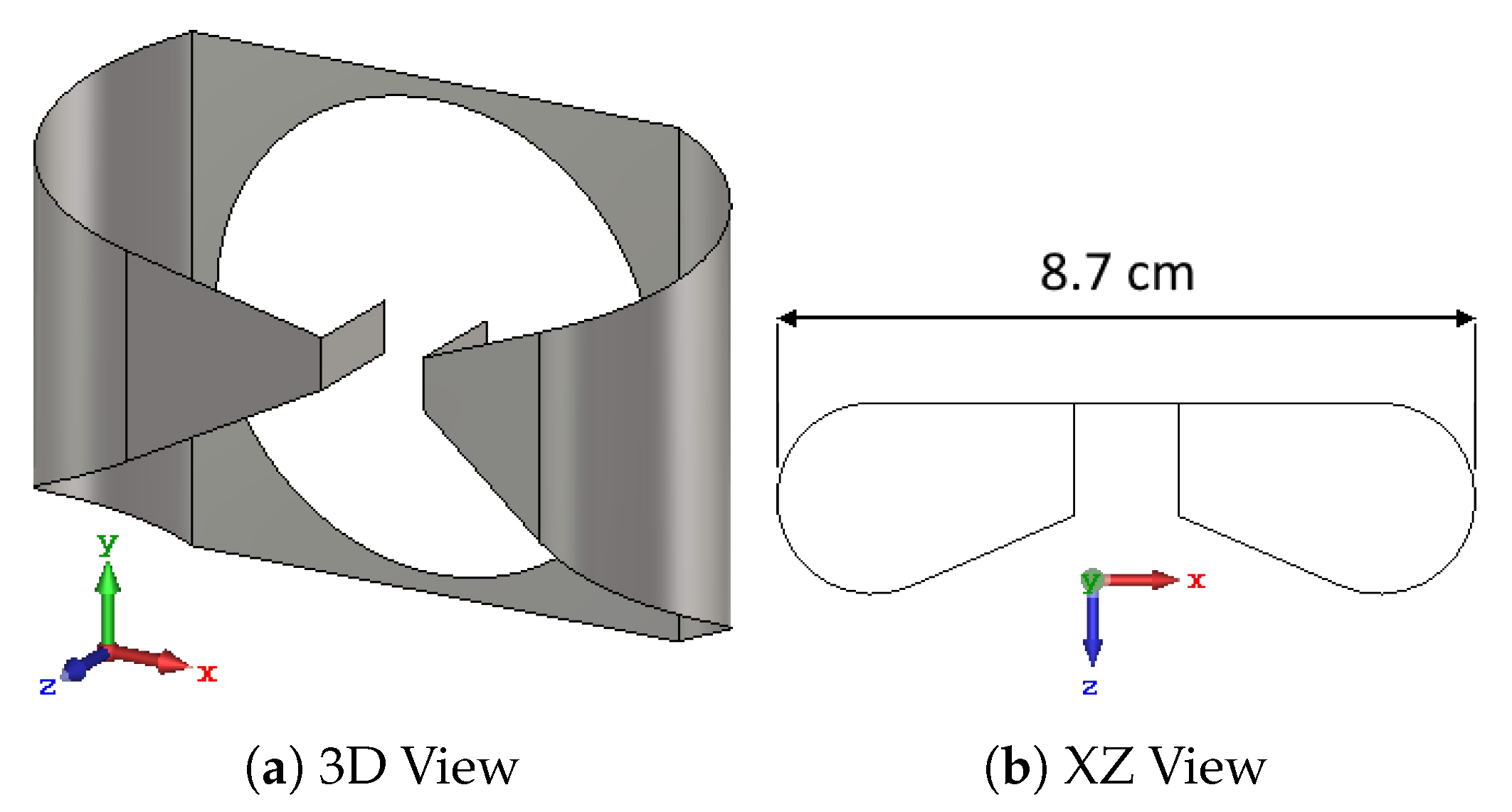
2.2. Antenna and Bolus Design
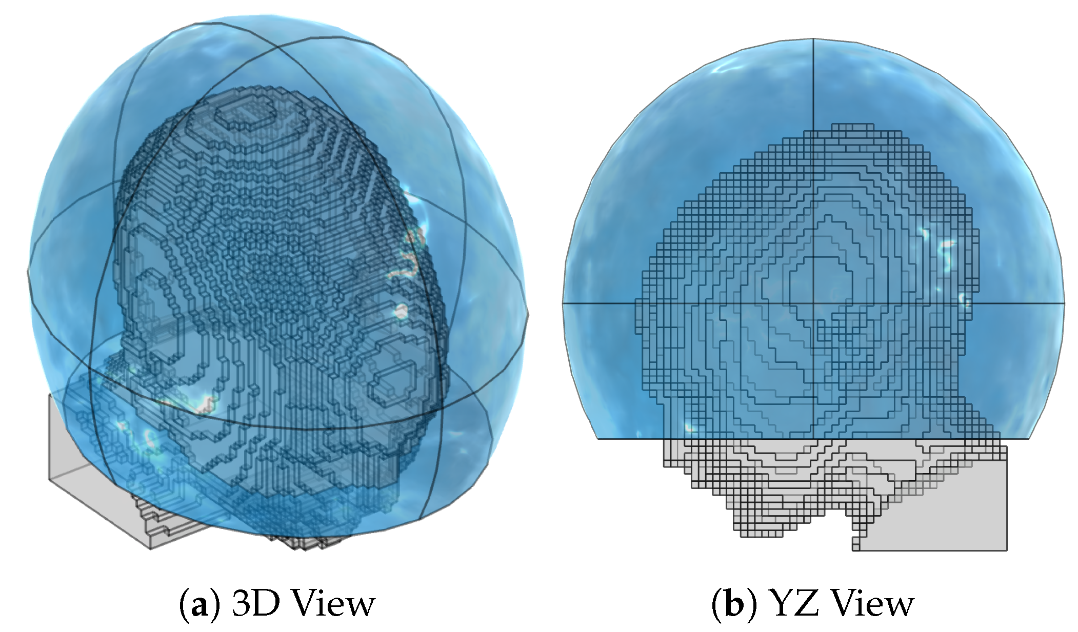
2.3. Numerical Simulations
2.4. Treatment Planning
2.5. Field Interpolation
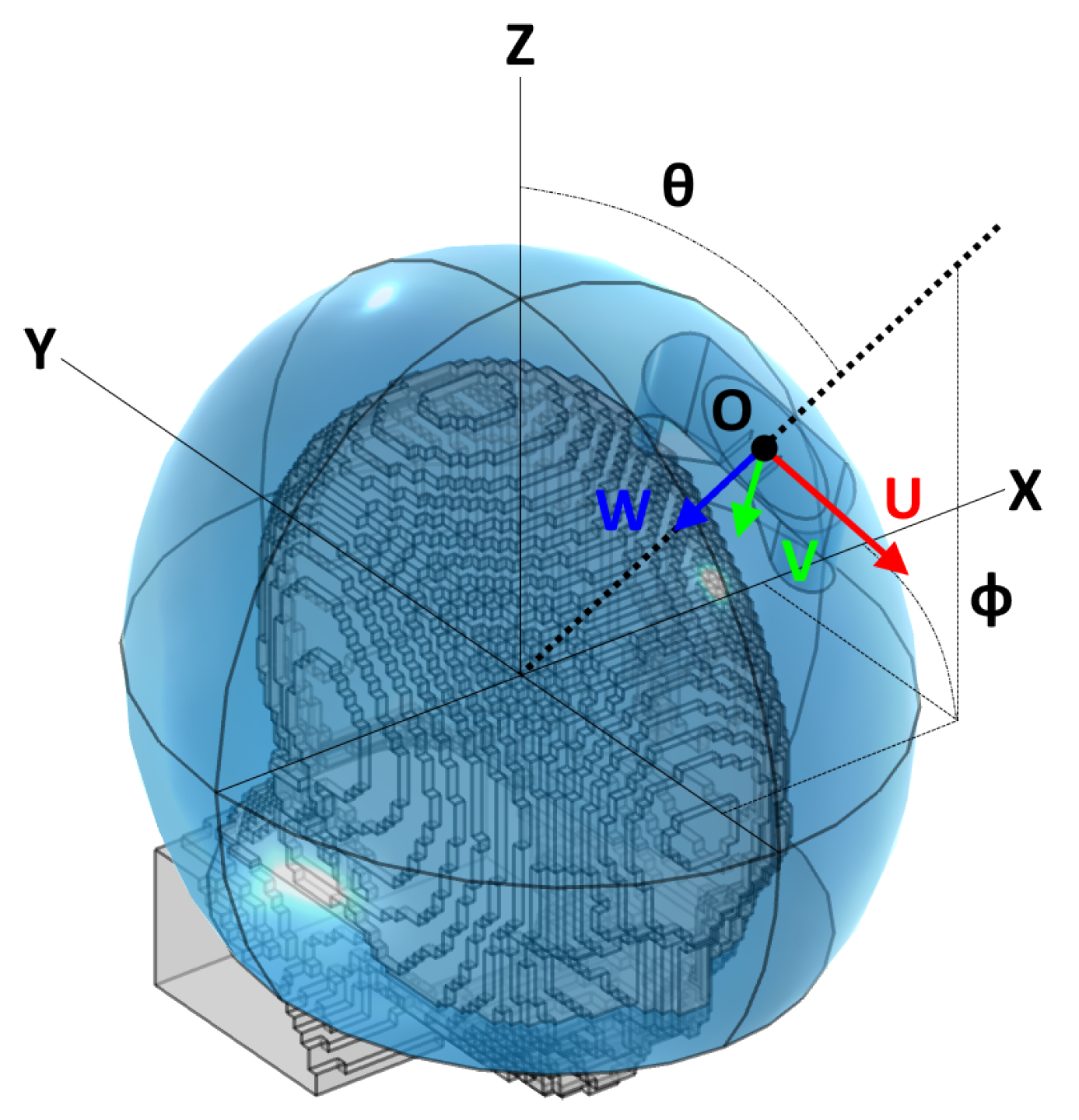
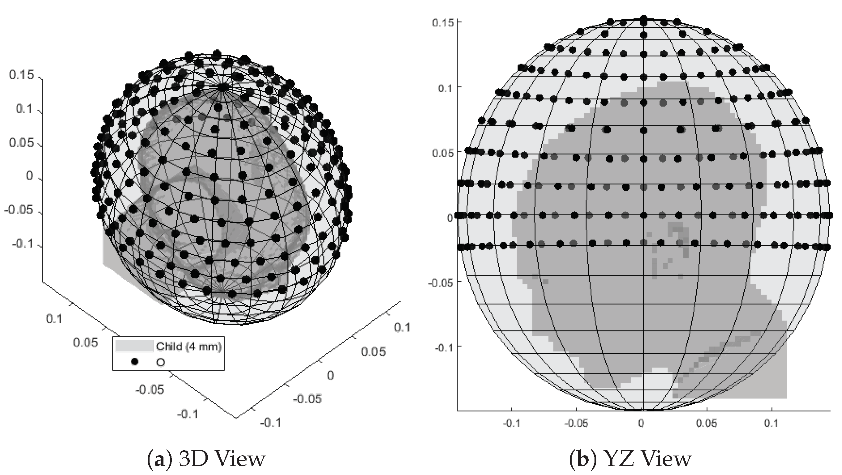
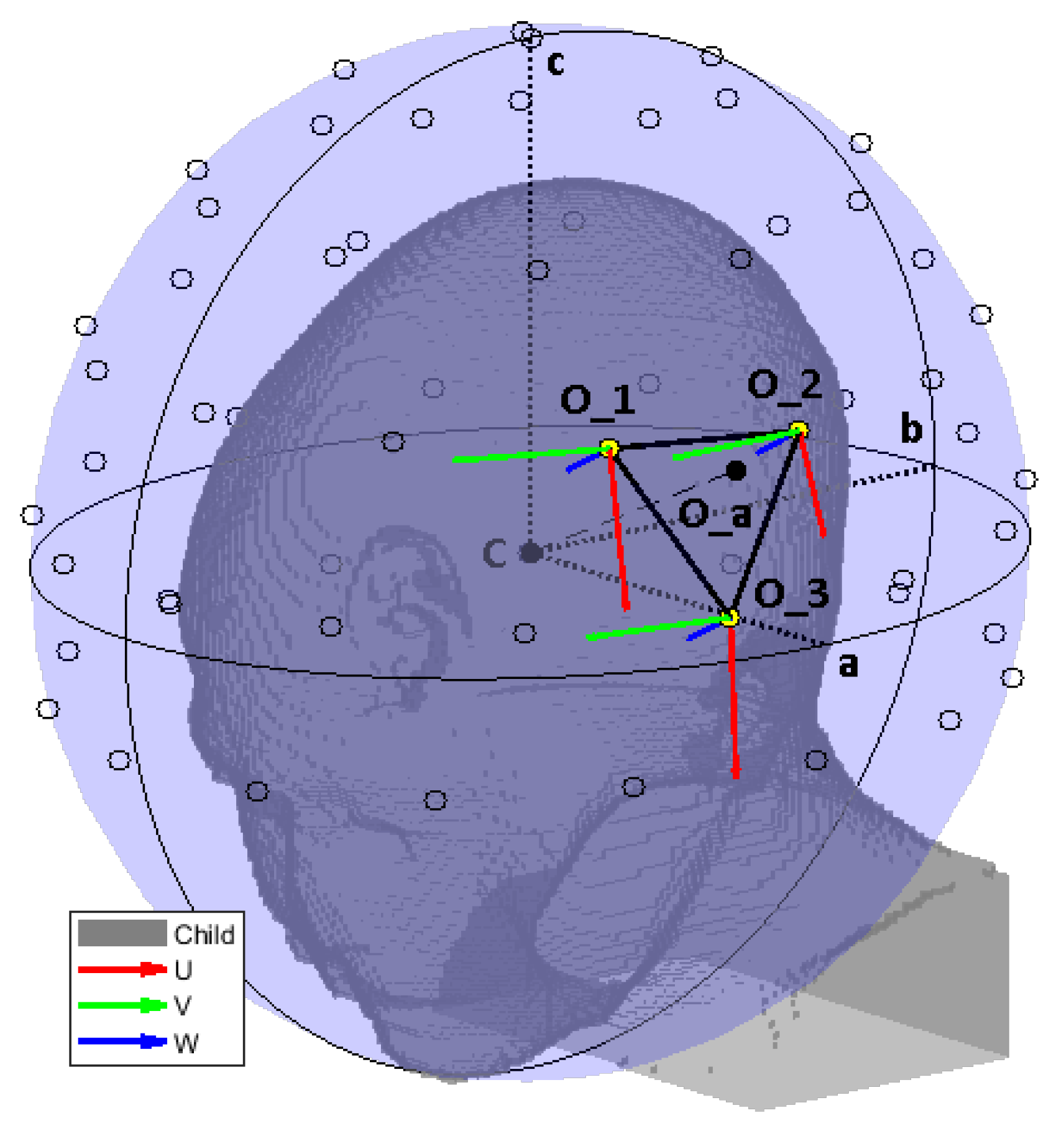
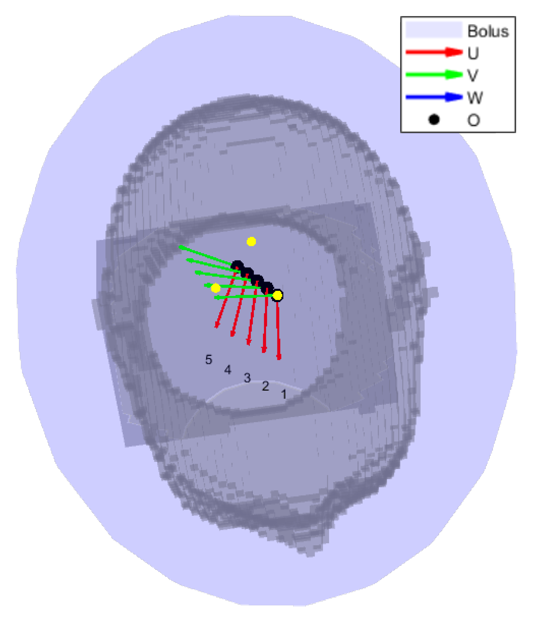
2.5.1. Interpolation Grid
2.5.2. Linear Interpolation
- 1.
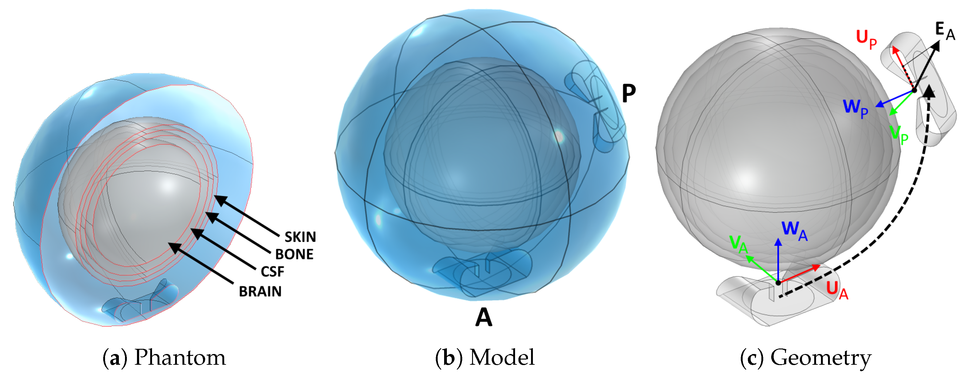
- A local coordinate system was built for the antenna, in a similar way to for the grid points in Section 2.5.1.
- 2.
- The complex vector E-field distribution of the first grid point at frequency f was divided everywhere by the local impedance of the material, yielding a surrogate of the H-field of an antenna at that location. This important step was included to render the field distribution less dependent on the patient’s anatomy, thanks to the biological tissues being predominantly non-magnetic.
- 3.
- This complex vector H-field distribution was transformed to according to a translation , a rotation , and a second translation , such that:
- 4.
- The transformed H-field distribution was multiplied by the material impedance to restore the transformed E-field intensity .
- 5.
- Steps 2 to 4 were repeated for each of the 3 closest grid points.
- 6.
- The E-field distribution relative to the individual antenna was obtained as a weighed average of the transformed distributions. The weights were determined as the ratio between the area of the subtended triangle to the area of the interpolation patch:where └⋄┐ denotes the area of the argument.
2.5.3. Coupling Modeling
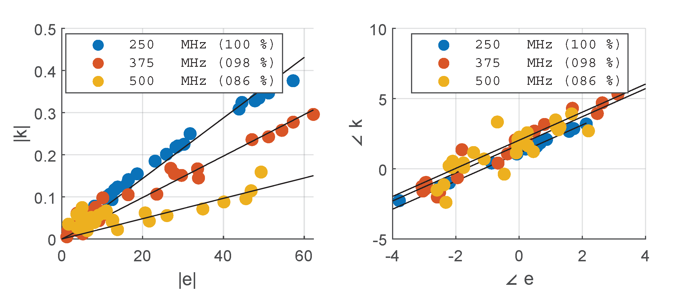
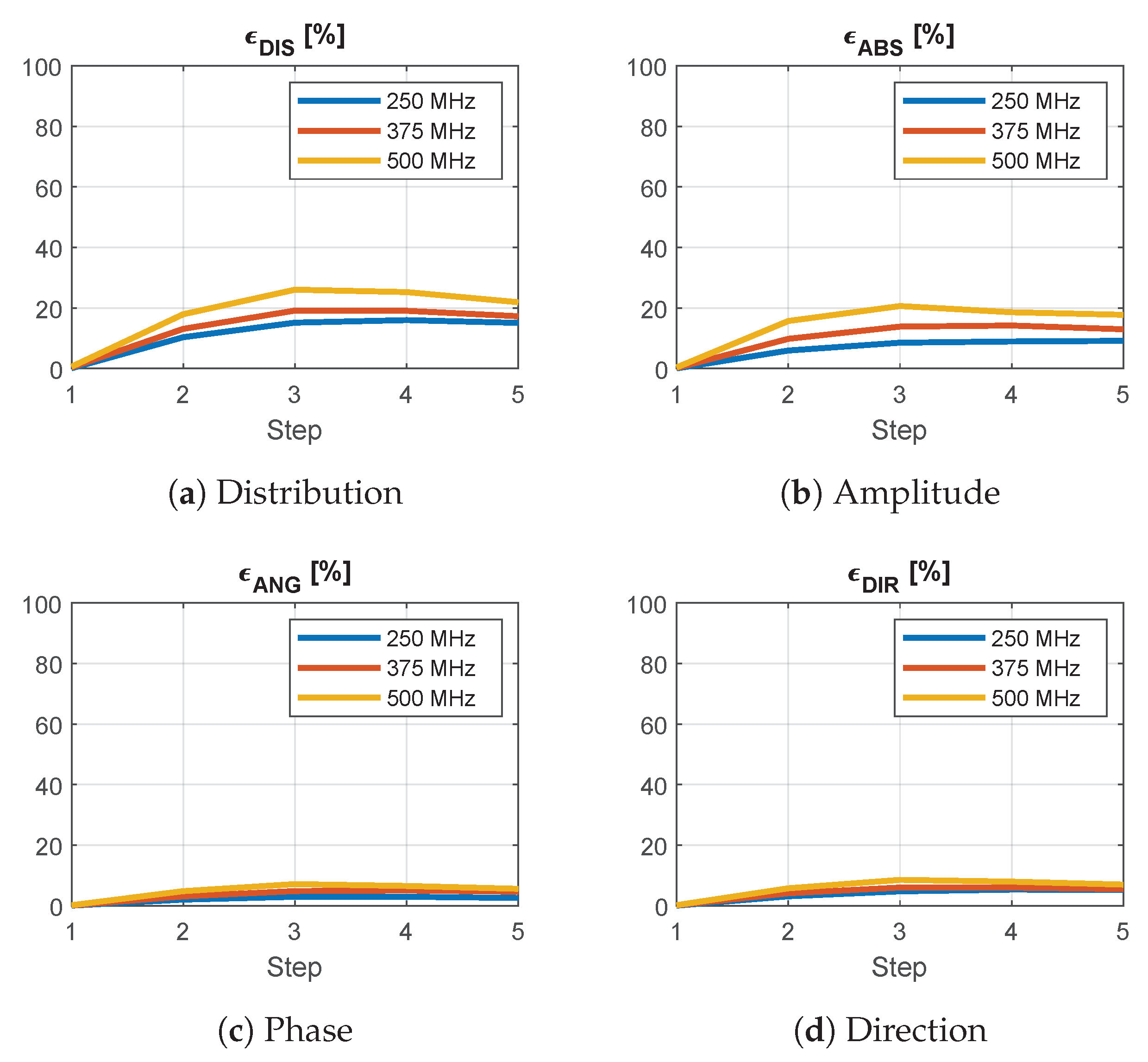
2.6. Approximation Analysis
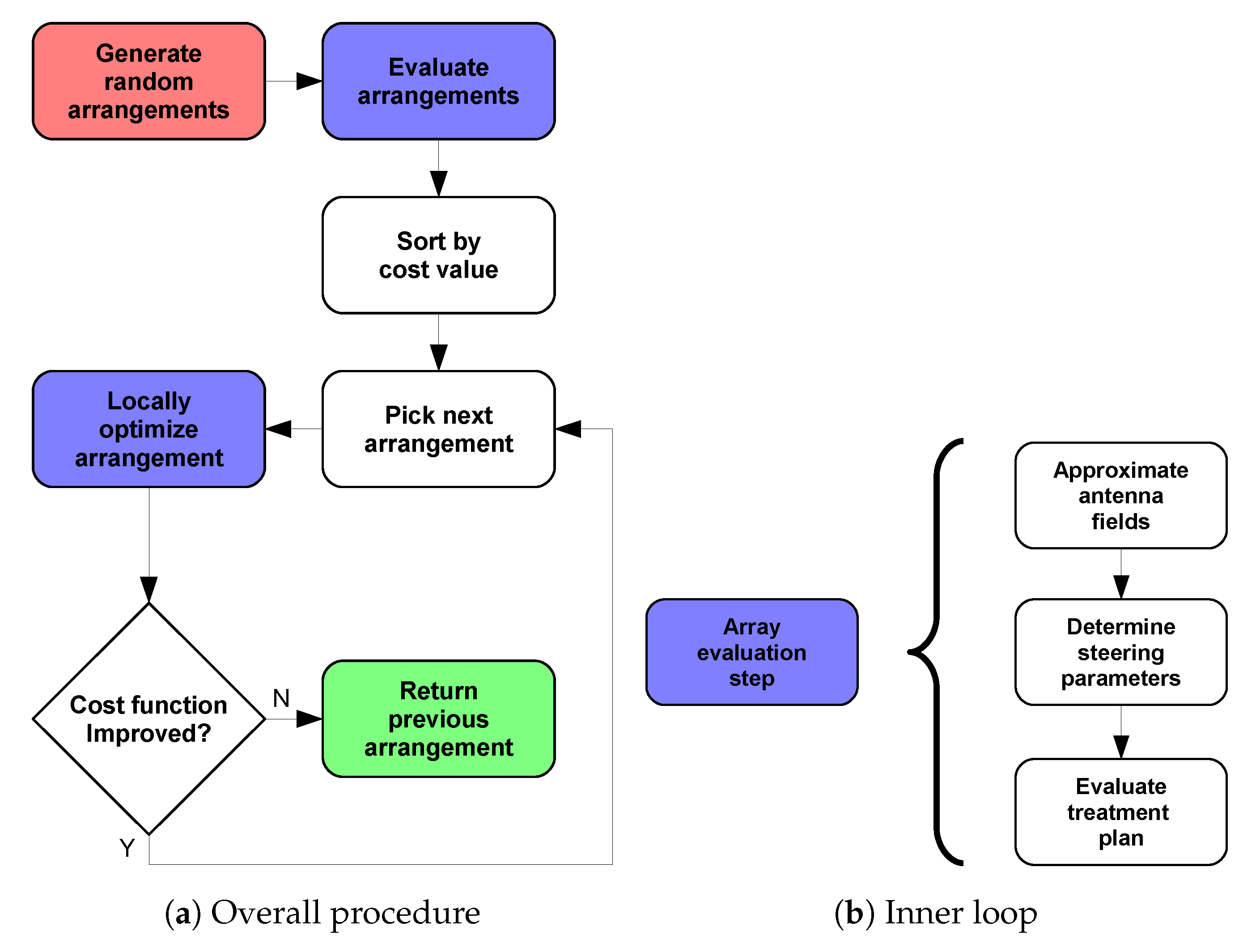
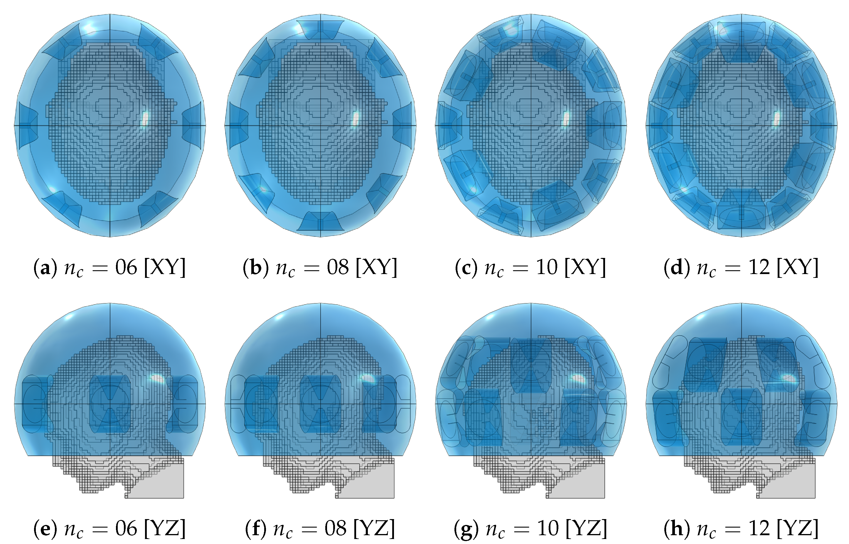
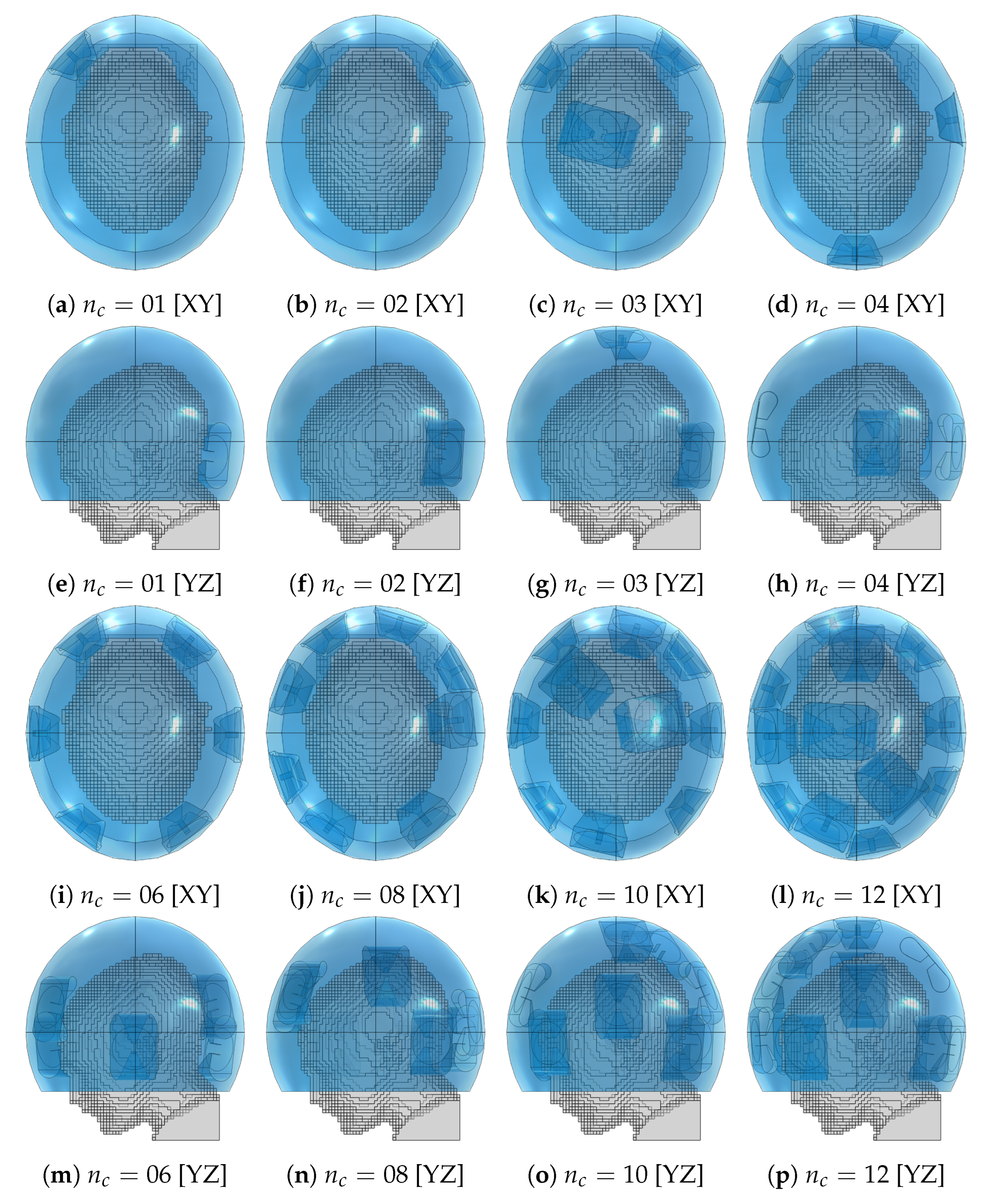
2.7. Array Optimization
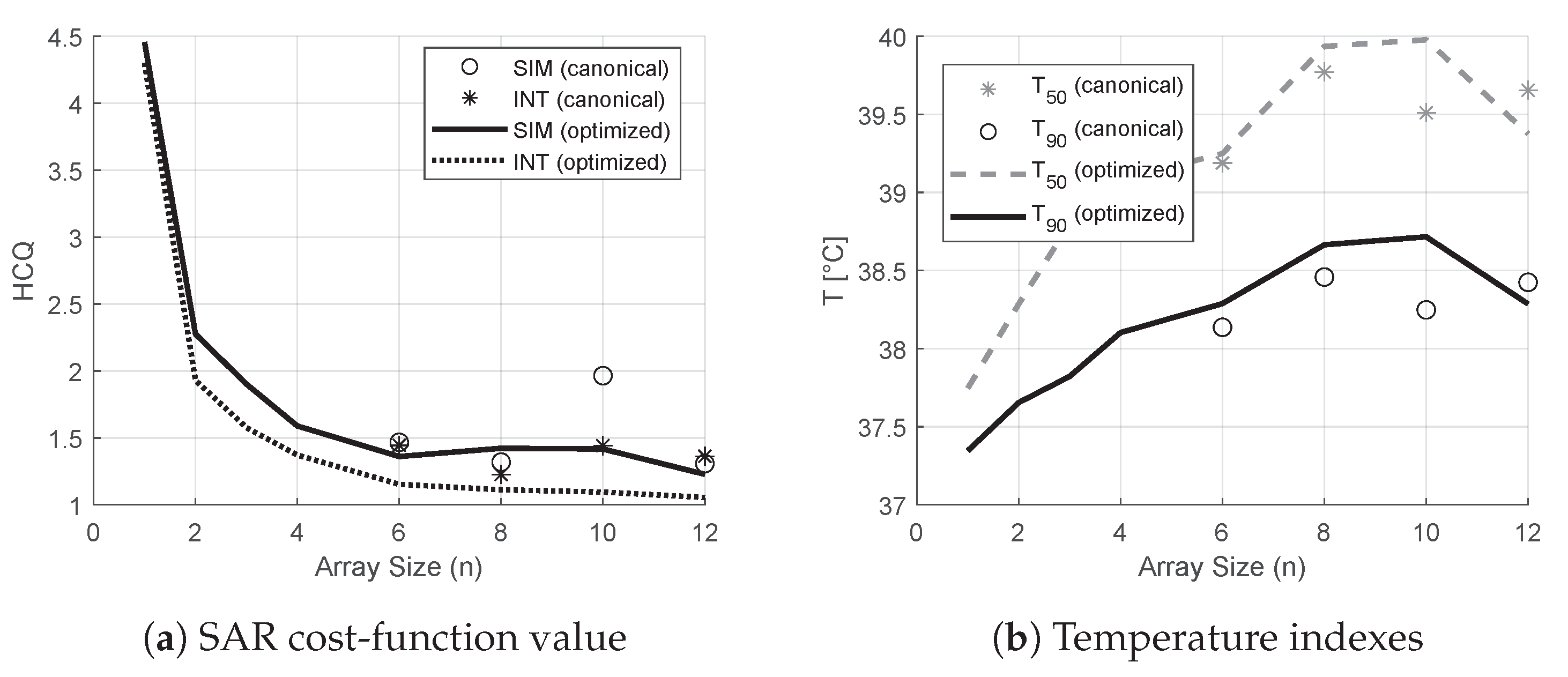
2.8. Design Validation
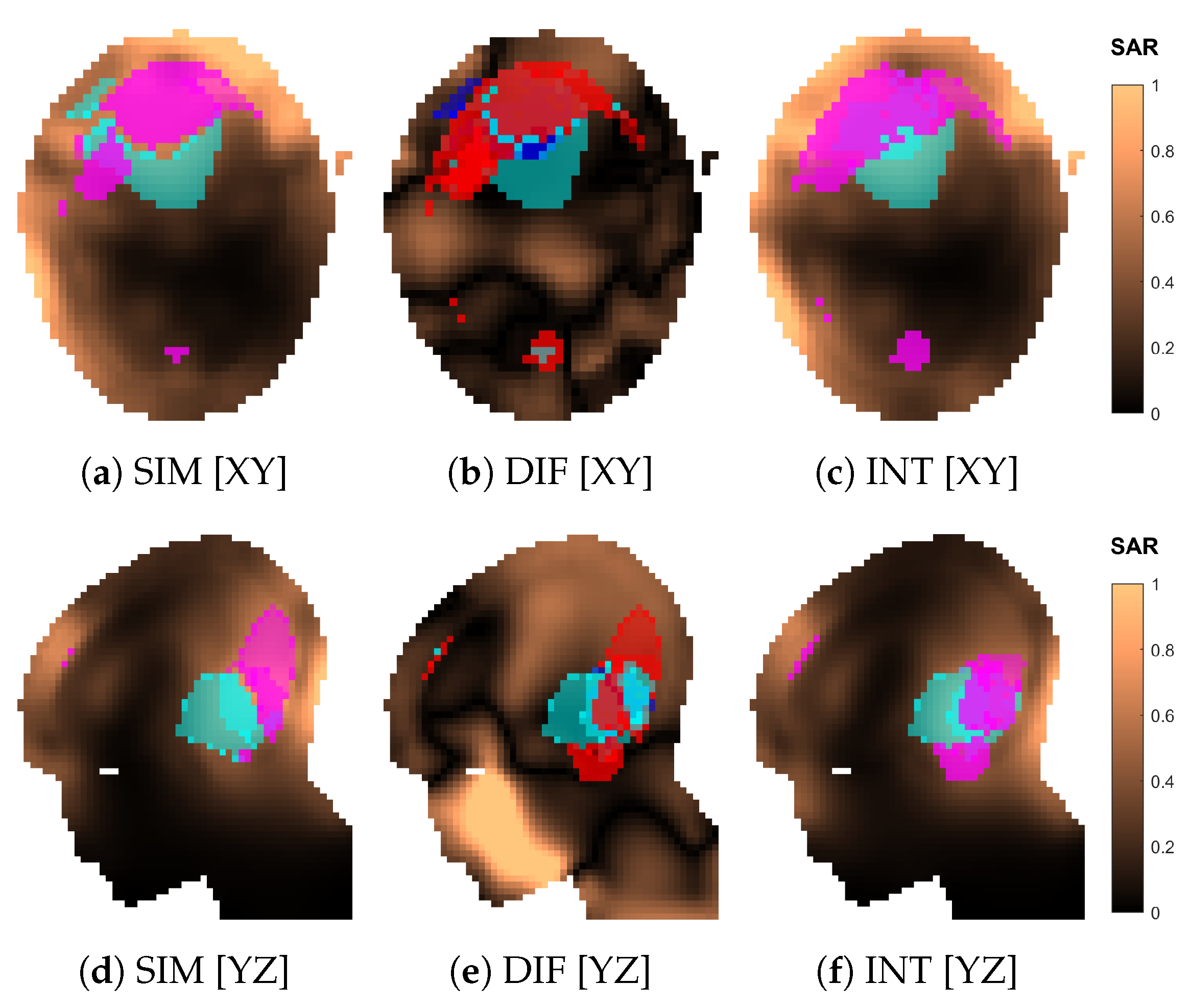
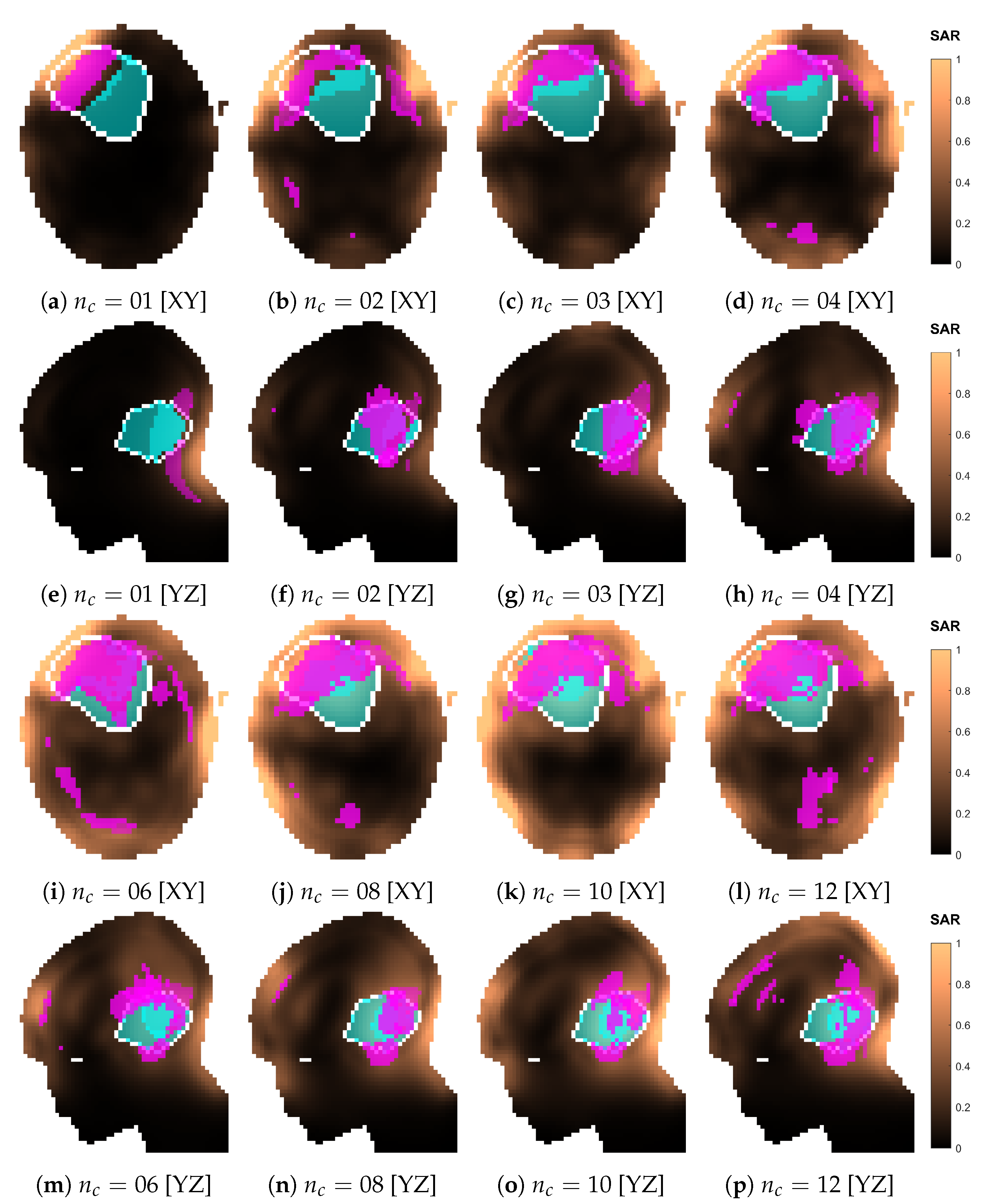
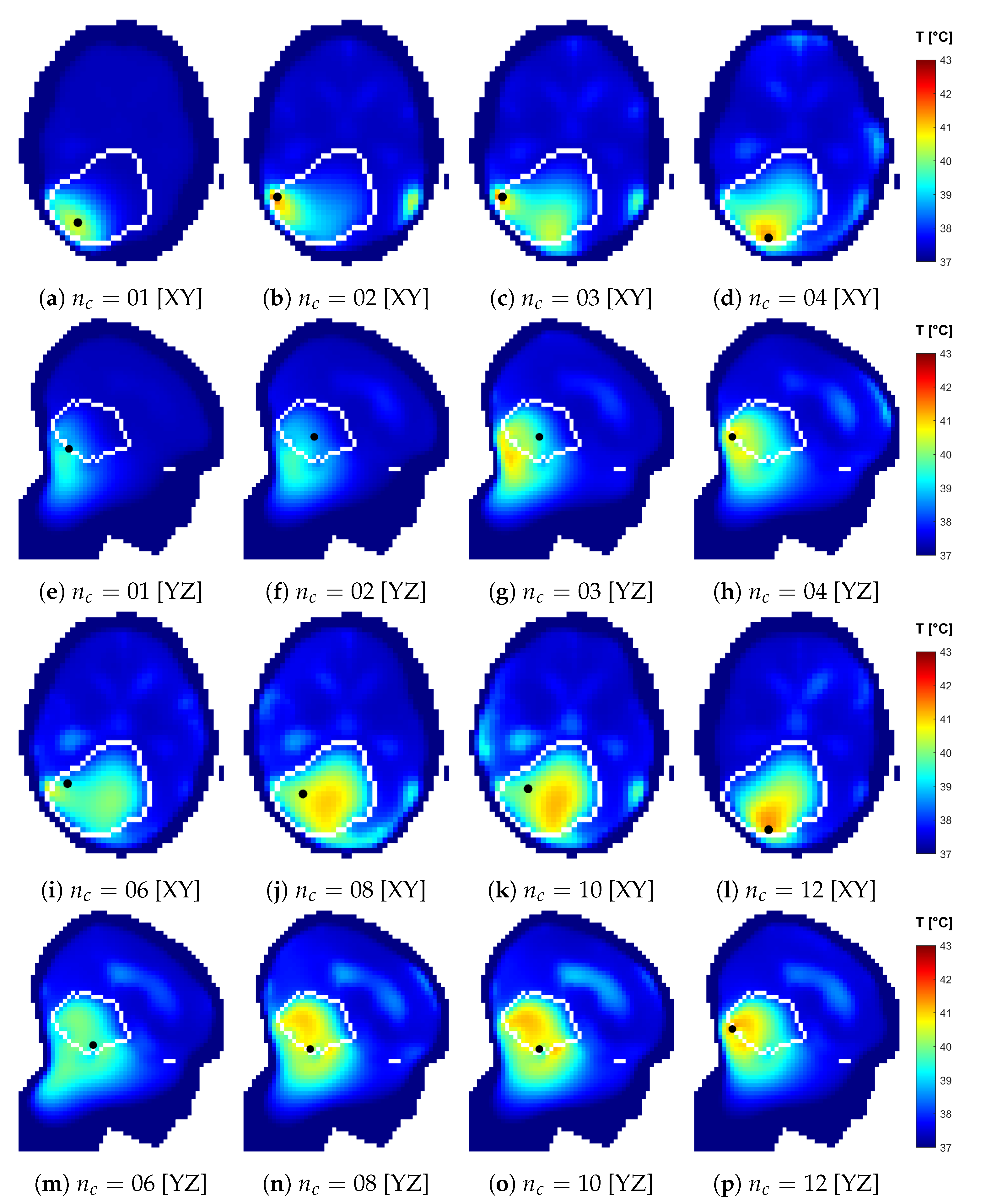
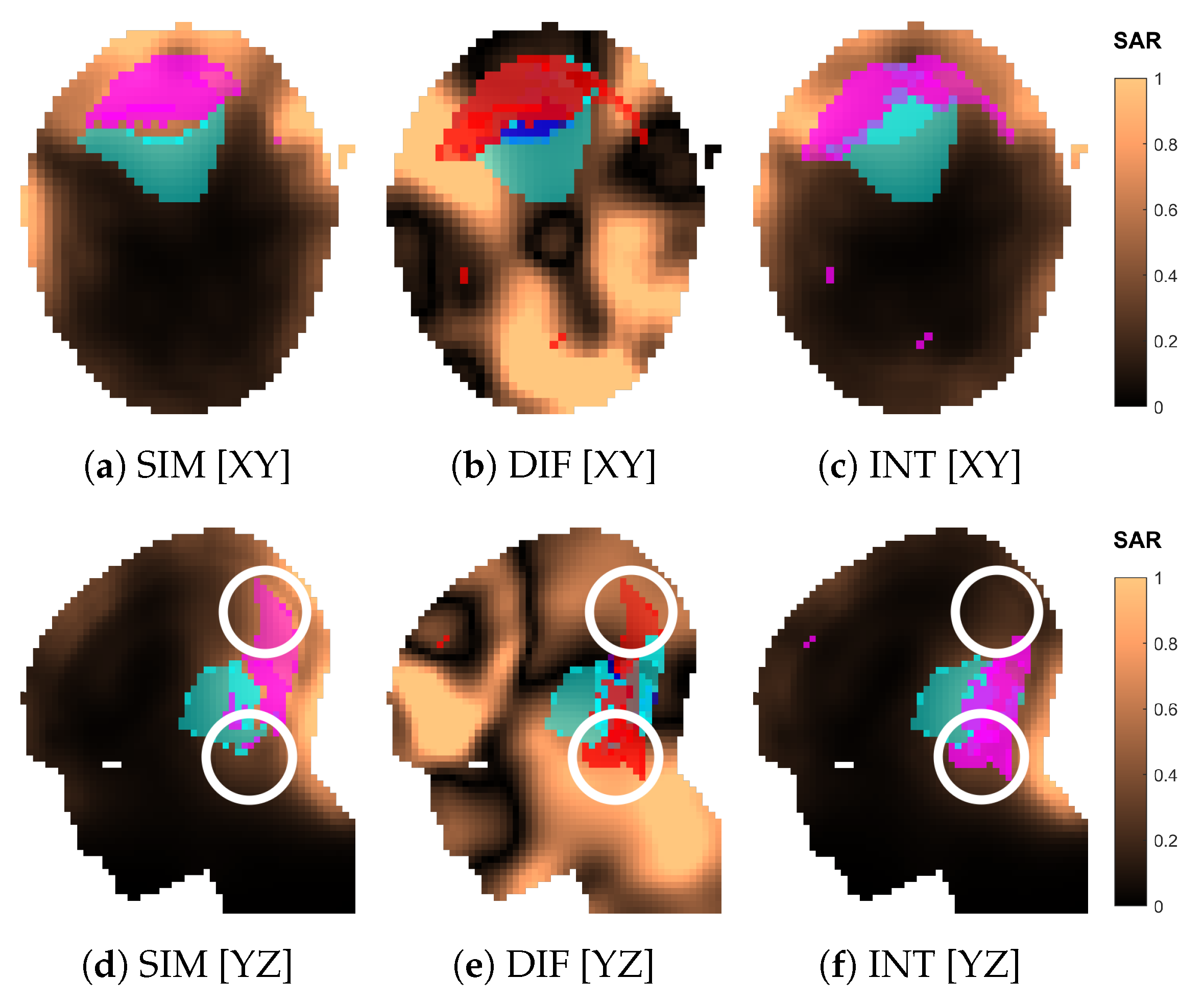
3. Results
Grid Simulation
4. Discussion
5. Conclusions
Author Contributions
Funding
Institutional Review Board Statement
Informed Consent Statement
Data Availability Statement
Acknowledgments
Conflicts of Interest
Abbreviations
| UWB | Ultra-wide band |
| MW | Microwave |
| HT | Hyperthermia |
| RF | Radio-frequency |
| CSF | Cerebrospinal fluid |
| BED | Biologically equivalent dose |
| HCQ | Hot-to-cold spot quotient |
| SAR | Specific absorption rate |
| PLD | Power loss density |
| HTV | Hyperthermia target volume |
| MRI | Magnetic resonance imaging |
| SGBT | Self-grounded bow tie |
| EM | Electromagnetic |
| TH | Thermal |
| PEC | Perfect electric conductor |
| TEM | Transverse electromagnetic |
| PML | Perfectly matched layer |
| GPU | Graphic processing unit |
| RAM | Random access memory |
| SIM | Simulated |
| INT | Interpolated |
| DIS | Distribution |
| ABS | Amplitude |
| ANG | Phase |
| DIR | Direction |
| DIF | Difference |
| RS | Random search |
| LR | Local refinement |
| CEM43T90 | Cumulative equivalent minutes at C using |
References
- Elming, P.B.; Sørensen, B.S.; Oei, A.L.; Franken, N.A.; Crezee, J.; Overgaard, J.; Horsman, M.R. Hyperthermia: The optimal treatment to overcome radiation resistant hypoxia. Cancers 2019, 11, 60. [Google Scholar] [CrossRef] [PubMed] [Green Version]
- Datta, N.; Ordóñez, S.G.; Gaipl, U.; Paulides, M.; Crezee, H.; Gellermann, J.; Marder, D.; Puric, E.; Bodis, S. Local hyperthermia combined with radiotherapy and-/or chemotherapy: Recent advances and promises for the future. Cancer Treat. Rev. 2015, 41, 742–753. [Google Scholar] [CrossRef] [PubMed]
- van der Horst, A.; Versteijne, E.; Besselink, M.G.; Daams, J.G.; Bulle, E.B.; Bijlsma, M.F.; Wilmink, J.W.; van Delden, O.M.; van Hooft, J.E.; Franken, N.A.; et al. The clinical benefit of hyperthermia in pancreatic cancer: A systematic review. Int. J. Hyperth. 2018, 34, 969–979. [Google Scholar] [CrossRef] [PubMed] [Green Version]
- Cihoric, N.; Tsikkinis, A.; van Rhoon, G.; Crezee, H.; Aebersold, D.M.; Bodis, S.; Beck, M.; Nadobny, J.; Budach, V.; Wust, P.; et al. Hyperthermia-related clinical trials on cancer treatment within the ClinicalTrials. gov registry. Int. J. Hyperth. 2015, 31, 609–614. [Google Scholar] [CrossRef]
- Kok, H.P.; Cressman, E.N.; Ceelen, W.; Brace, C.L.; Ivkov, R.; Grüll, H.; Ter Haar, G.; Wust, P.; Crezee, J. Heating technology for malignant tumors: A review. Int. J. Hyperth. 2020, 37, 711–741. [Google Scholar] [CrossRef]
- Bakker, A.; van der Zee, J.; van Tienhoven, G.; Kok, H.P.; Rasch, C.R.; Crezee, H. Temperature and thermal dose during radiotherapy and hyperthermia for recurrent breast cancer are related to clinical outcome and thermal toxicity: A systematic review. Int. J. Hyperth. 2019, 36, 1023–1038. [Google Scholar] [CrossRef] [Green Version]
- Sneed, P.K.; Gutin, P.H.; Stauffer, P.R.; Phillips, T.L.; Prados, M.D.; Weaver, K.A.; Suen, S.; Lamb, S.A.; Ham, B.; Ahn, D.K.; et al. Thermoradiotherapy of recurrent malignant brain tumors. Int. J. Radiat. Oncol. Biol. Phys. 1992, 23, 853–861. [Google Scholar] [CrossRef]
- McNeill, K.A. Epidemiology of brain tumors. Neurol. Clin. 2016, 34, 981–998. [Google Scholar] [CrossRef]
- Makale, M.T.; McDonald, C.R.; Hattangadi-Gluth, J.A.; Kesari, S. Mechanisms of radiotherapy-associated cognitive disability in patients with brain tumours. Nat. Rev. Neurol. 2017, 13, 52–64. [Google Scholar] [CrossRef] [Green Version]
- Haveman, J.; Sminia, P.; Wondergem, J.; van der Zee, J.; Hulshof, M. Effects of hyperthermia on the central nervous system: What was learnt from animal studies? Int. J. Hyperth. 2005, 21, 473–487. [Google Scholar] [CrossRef]
- Cutz, A. Effects of microwave radiation on the eye: The occupational health perspective. Lens Eye Toxic. Res. 1989, 6, 379–386. [Google Scholar] [PubMed]
- Fessenden, P.; Hand, J.W. Hyperthermia therapy physics. In Radiation Therapy Physics; Springer: Berlin/Heidelberg, Germany, 1995; pp. 315–363. [Google Scholar]
- Hasgall, P.; Di Gennaro, F.; Baumgartner, C.; Neufeld, E.; Lloyd, B.; Gosselin, M.; Payne, D.; Klingenböck, A.; Kuster, N. IT’IS Database for Thermal and Electromagnetic Parameters of Biological Tissues; IT’IS Foundation: Zurich, Switzerland, 2018. [Google Scholar]
- Shoji, H.; Motegi, M.; Osawa, K.; Okonogi, N.; Okazaki, A.; Andou, Y.; Asao, T.; Kuwano, H.; Takahashi, T.; Ogoshi, K. Output-limiting symptoms induced by radiofrequency hyperthermia. Are they predictable? Int. J. Hyperth. 2016, 32, 199–203. [Google Scholar] [CrossRef] [PubMed] [Green Version]
- Van der Gaag, M.; De Bruijne, M.; Samaras, T.; Van Der Zee, J.; Van Rhoon, G. Development of a guideline for the water bolus temperature in superficial hyperthermia. Int. J. Hyperth. 2006, 22, 637–656. [Google Scholar] [CrossRef] [PubMed]
- Seebass, M.; Beck, R.; Gellermann, J.; Nadobny, J.; Wust, P. Electromagnetic phased arrays for regional hyperthermia: Optimal frequency and antenna arrangement. Int. J. Hyperth. 2001, 17, 321–336. [Google Scholar] [CrossRef] [PubMed]
- Paulides, M.M.; Vossen, S.H.; Zwamborn, A.P.; van Rhoon, G.C. Theoretical investigation into the feasibility to deposit RF energy centrally in the head-and-neck region. Int. J. Radiat. Oncol. Biol. Phys. 2005, 63, 634–642. [Google Scholar] [CrossRef] [PubMed]
- Crezee, J.; Van Haaren, P.; Westendorp, H.; De Greef, M.; Kok, H.; Wiersma, J.; Van Stam, G.; Sijbrands, J.; Zum Vörde Sive Vörding, P.; Van Dijk, J.; et al. Improving locoregional hyperthermia delivery using the 3-D controlled AMC-8 phased array hyperthermia system: A preclinical study. Int. J. Hyperth. 2009, 25, 581–592. [Google Scholar] [CrossRef] [PubMed]
- Kok, H.; De Greef, M.; Borsboom, P.; Bel, A.; Crezee, J. Improved power steering with double and triple ring waveguide systems: The impact of the operating frequency. Int. J. Hyperth. 2011, 27, 224–239. [Google Scholar] [CrossRef]
- Togni, P.; Rijnen, Z.; Numan, W.; Verhaart, R.; Bakker, J.; Van Rhoon, G.; Paulides, M. Electromagnetic redesign of the HYPERcollar applicator: Toward improved deep local head-and-neck hyperthermia. Phys. Med. Biol. 2013, 58, 5997. [Google Scholar] [CrossRef]
- Skandalakis, G.P.; Rivera, D.R.; Rizea, C.D.; Bouras, A.; Jesu Raj, J.G.; Bozec, D.; Hadjipanayis, C.G. Hyperthermia treatment advances for brain tumors. Int. J. Hyperth. 2020, 37, 3–19. [Google Scholar] [CrossRef]
- Rodrigues, D.B.; Ellsworth, J.; Turner, P. Feasibility of heating brain tumors using a 915 MHz annular phased-array. IEEE Antennas Wirel. Propag. Lett. 2021, 20, 423–427. [Google Scholar] [CrossRef]
- Oberacker, E.; Kuehne, A.; Nadobny, J.; Zschaeck, S.; Weihrauch, M.; Waiczies, H.; Ghadjar, P.; Wust, P.; Niendorf, T.; Winter, L. Radiofrequency applicator concepts for simultaneous MR imaging and hyperthermia treatment of glioblastoma multiforme. Curr. Dir. Biomed. Eng. 2017, 3, 473–477. [Google Scholar] [CrossRef] [Green Version]
- Takook, P.; Persson, M.; Trefná, H.D. Performance evaluation of hyperthermia applicators to heat deep-seated brain tumors. IEEE J. Electromagn. RF Microwaves Med. Biol. 2018, 2, 18–24. [Google Scholar] [CrossRef]
- Oberacker, E.; Diesch, C.; Nadobny, J.; Kuehne, A.; Wust, P.; Ghadjar, P.; Niendorf, T. Patient-specific planning for thermal magnetic resonance of glioblastoma multiforme. Cancers 2021, 13, 1867. [Google Scholar] [CrossRef] [PubMed]
- Ghaderi Aram, M.; Zanoli, M.; Nordström, H.; Toma-Dasu, I.; Blomgren, K.; Dobšíček Trefná, H. Radiobiological Evaluation of Combined Gamma Knife Radiosurgery and Hyperthermia for Pediatric Neuro-Oncology. Cancers 2021, 13, 3277. [Google Scholar] [CrossRef] [PubMed]
- Zanoli, M.; Trefná, H.D. Combining target coverage and hot-spot suppression into one cost function: The hot-to-cold spot quotient. In Proceedings of the 2021 15th European Conference on Antennas and Propagation (EuCAP), Dusseldorf, Germany, 22–26 March 2021; pp. 1–4. [Google Scholar]
- Zanoli, M.; Dobšíček Trefná, H. The hot-to-cold spot quotient for SAR-based treatment planning in deep microwave hyperthermia. Int. J. Hyperth. 2022, 39, 1421–1439. [Google Scholar] [CrossRef] [PubMed]
- Takook, P.; Persson, M.; Gellermann, J.; Trefná, H.D. Compact self-grounded Bow-Tie antenna design for an UWB phased-array hyperthermia applicator. Int. J. Hyperth. 2017, 33, 387–400. [Google Scholar] [CrossRef] [PubMed]
- COMSOL AB. COMSOL Multiphysics® v. 5.6; COMSOL AB: Stockholm, Sweden, 2020. [Google Scholar]
- James, B.J.; Sullivan, D.M. Creation of three-dimensional patient models for hyperthermia treatment planning. IEEE Trans. Biomed. Eng. 1992, 39, 238–242. [Google Scholar] [CrossRef]
- Joines, W.T.; Zhang, Y.; Li, C.; Jirtle, R.L. The measured electrical properties of normal and malignant human tissues from 50 to 900 MHz. Med Phys. 1994, 21, 547–550. [Google Scholar] [CrossRef]
- Paulides, M.M.; Rodrigues, D.B.; Bellizzi, G.G.; Sumser, K.; Curto, S.; Neufeld, E.; Montanaro, H.; Kok, H.P.; Dobsicek Trefna, H. ESHO benchmarks for computational modeling and optimization in hyperthermia therapy. Int. J. Hyperth. 2021, 38, 1425–1442. [Google Scholar] [CrossRef]
- Verhaart, R.F.; Verduijn, G.M.; Fortunati, V.; Rijnen, Z.; van Walsum, T.; Veenland, J.F.; Paulides, M.M. Accurate 3D temperature dosimetry during hyperthermia therapy by combining invasive measurements and patient-specific simulations. Int. J. Hyperth. 2015, 31, 686–692. [Google Scholar] [CrossRef] [Green Version]
- Pennes, H.H. Analysis of tissue and arterial blood temperatures in the resting human forearm. J. Appl. Physiol. 1948, 1, 93–122. [Google Scholar] [CrossRef] [PubMed]
- Bruggmoser, G.; Bauchowitz, S.; Canters, R.; Crezee, H.; Ehmann, M.; Gellermann, J.; Lamprecht, U.; Lomax, N.; Messmer, M.B.; Ott, O.; et al. Quality assurance for clinical studies in regional deep hyperthermia. Strahlenther. Und Onkol. 2011, 187, 605–610. [Google Scholar] [CrossRef] [PubMed] [Green Version]
- The MathWorks Inc. MATLAB R2021; The MathWorks Inc.: Natick, MA, USA, 2021. [Google Scholar]
- Zanoli, M.; Trefná, H.D. Iterative time-reversal for multi-frequency hyperthermia. Phys. Med. Biol. 2021, 66, 045027. [Google Scholar] [CrossRef] [PubMed]
- Bakker, J.; Paulides, M.; Neufeld, E.; Christ, A.; Kuster, N.; Van Rhoon, G. Children and adults exposed to electromagnetic fields at the ICNIRP reference levels: Theoretical assessment of the induced peak temperature increase. Phys. Med. Biol. 2011, 56, 4967. [Google Scholar] [CrossRef]
- Romeijn, H.E. Random Search Methods. In Encyclopedia of Optimization; Floudas, C.A., Pardalos, P.M., Eds.; Springer: Boston, MA, USA, 2009; pp. 3245–3251. [Google Scholar] [CrossRef]
- Kroesen, M.; Mulder, H.T.; van Holthe, J.M.; Aangeenbrug, A.A.; Mens, J.W.M.; van Doorn, H.C.; Paulides, M.M.; Oomen-de Hoop, E.; Vernhout, R.M.; Lutgens, L.C.; et al. Confirmation of thermal dose as a predictor of local control in cervical carcinoma patients treated with state-of-the-art radiation therapy and hyperthermia. Radiother. Oncol. 2019, 140, 150–158. [Google Scholar] [CrossRef]
- van Rhoon, G.C. Is CEM43 still a relevant thermal dose parameter for hyperthermia treatment monitoring? Int. J. Hyperth. 2016, 32, 50–62. [Google Scholar] [CrossRef]
- Kok, H.; Schooneveldt, G.; Bakker, A.; de Kroon-Oldenhof, R.; Korshuize-van Straten, L.; De Jong, C.; Steggerda-Carvalho, E.; Geijsen, E.; Stalpers, L.; Crezee, J. Predictive value of simulated SAR and temperature for changes in measured temperature after phase-amplitude steering during locoregional hyperthermia treatments. Int. J. Hyperth. 2018, 35, 330–339. [Google Scholar] [CrossRef] [Green Version]
- Verhaart, R.F.; Fortunati, V.; Verduijn, G.M.; van der Lugt, A.; van Walsum, T.; Veenland, J.F.; Paulides, M.M. The relevance of MRI for patient modeling in head and neck hyperthermia treatment planning: A comparison of CT and CT-MRI based tissue segmentation on simulated temperature. Med Phys. 2014, 41, 123302. [Google Scholar] [CrossRef]
- Schooneveldt, G.; Dobšícek Trefná, H.; Persson, M.; de Reijke, T.M.; Blomgren, K.; Kok, H.P.; Crezee, H. Hyperthermia treatment planning including convective flow in cerebrospinal fluid for brain tumour hyperthermia treatment using a novel dedicated paediatric brain applicator. Cancers 2019, 11, 1183. [Google Scholar] [CrossRef] [Green Version]
- Aklan, B.; Gierse, P.; Hartmann, J.; Ott, O.J.; Fietkau, R.; Bert, C. Influence of patient mispositioning on SAR distribution and simulated temperature in regional deep hyperthermia. Phys. Med. Biol. 2017, 62, 4929. [Google Scholar] [CrossRef]
- Aklan, B.; Zilles, B.; Paprottka, P.; Manz, K.; Pfirrmann, M.; Santl, M.; Abdel-Rahman, S.; Lindner, L. Regional deep hyperthermia: Quantitative evaluation of predicted and direct measured temperature distributions in patients with high-risk extremity soft-tissue sarcoma. Int. J. Hyperth. 2019, 36, 169–184. [Google Scholar] [CrossRef] [PubMed]


| (OPT) | 08 | 98 | 99 |
| (OPT) | 32 | 80 | 95 |
| (OPT) | 36 | 79 | 96 |
| (OPT) | 22 | 63 | 87 |
| (OPT) | 28 | 54 | 84 |
| (OPT) | 29 | 46 | 81 |
| (OPT) | 32 | 46 | 82 |
| (OPT) | 28 | 65 | 84 |
| (CAN) | 26 | 46 | 88 |
| (CAN) | 20 | 69 | 91 |
| (CAN) | 58 | 41 | 84 |
| (CAN) | 25 | 57 | 85 |
| (OPT) | 42 | 62 | 86 |
| (OPT) | 34 | 71 | 94 |
| (OPT) | 28 | 65 | 84 |
| (OPT) | 29 | 72 | 95 |
| (OPT) | 28 | 44 | 78 |
| POWER [%] | 250 MHz | 375 MHz | 500 MHz | Antenna Total: |
|---|---|---|---|---|
| Ant. 01 | 06 | 04 | 05 | 15 |
| Ant. 02 | 00 | 00 | 00 | 00 |
| Ant. 03 | 02 | 01 | 03 | 05 |
| Ant. 04 | 07 | 08 | 02 | 17 |
| Ant. 05 | 16 | 05 | 02 | 23 |
| Ant. 06 | 03 | 01 | 02 | 06 |
| Ant. 07 | 01 | 06 | 03 | 10 |
| Ant. 08 | 01 | 03 | 04 | 09 |
| Ant. 09 | 05 | 01 | 04 | 09 |
| Ant. 10 | 04 | 01 | 02 | 07 |
| Frequency total: | 44 | 30 | 26 |
| 250 MHz | 375 MHz | 500 MHz | 250 MHz | 375 MHz | 500 MHz | ||
| Ant. 01 | 144 | 099 | 080 | Ant. 01 | 109 | 071 | 046 |
| Ant. 02 | 201 | 134 | 106 | Ant. 02 | 171 | 117 | 072 |
| Ant. 03 | 153 | 111 | 091 | Ant. 03 | 127 | 094 | 069 |
| Ant. 04 | 152 | 106 | 080 | Ant. 04 | 121 | 071 | 051 |
| Ant. 05 | 150 | 113 | 074 | Ant. 05 | 091 | 095 | 062 |
| Ant. 06 | 179 | 155 | 096 | Ant. 06 | 151 | 119 | 088 |
| Ant. 07 | 221 | 161 | 101 | Ant. 07 | 185 | 114 | 102 |
| Ant. 08 | 155 | 157 | 088 | Ant. 08 | 104 | 105 | 063 |
| Ant. 09 | 156 | 150 | 096 | Ant. 09 | 160 | 111 | 095 |
| Ant. 10 | 151 | 144 | 086 | Ant. 10 | 116 | 101 | 055 |
| MEAN: | 166 | 133 | 090 | MEAN: | 133 | 100 | 070 |
| 250 MHz | 375 MHz | 500 MHz | 250 MHz | 375 MHz | 500 MHz | ||
| Ant. 01 | 026 | 022 | 018 | Ant. 01 | 023 | 022 | 022 |
| Ant. 02 | 040 | 035 | 026 | Ant. 02 | 024 | 027 | 024 |
| Ant. 03 | 032 | 026 | 025 | Ant. 03 | 024 | 025 | 024 |
| Ant. 04 | 027 | 022 | 020 | Ant. 04 | 023 | 025 | 021 |
| Ant. 05 | 028 | 023 | 018 | Ant. 05 | 024 | 024 | 021 |
| Ant. 06 | 028 | 030 | 032 | Ant. 06 | 023 | 024 | 025 |
| Ant. 07 | 032 | 035 | 032 | Ant. 07 | 022 | 025 | 025 |
| Ant. 08 | 026 | 031 | 027 | Ant. 08 | 022 | 023 | 021 |
| Ant. 09 | 030 | 033 | 025 | Ant. 09 | 021 | 024 | 023 |
| Ant. 10 | 025 | 029 | 025 | Ant. 10 | 021 | 024 | 023 |
| MEAN: | 029 | 029 | 025 | MEAN: | 023 | 025 | 023 |
Disclaimer/Publisher’s Note: The statements, opinions and data contained in all publications are solely those of the individual author(s) and contributor(s) and not of MDPI and/or the editor(s). MDPI and/or the editor(s) disclaim responsibility for any injury to people or property resulting from any ideas, methods, instructions or products referred to in the content. |
© 2023 by the authors. Licensee MDPI, Basel, Switzerland. This article is an open access article distributed under the terms and conditions of the Creative Commons Attribution (CC BY) license (https://creativecommons.org/licenses/by/4.0/).
Share and Cite
Zanoli, M.; Ek, E.; Dobšíček Trefná, H. Antenna Arrangement in UWB Helmet Brain Applicators for Deep Microwave Hyperthermia. Cancers 2023, 15, 1447. https://doi.org/10.3390/cancers15051447
Zanoli M, Ek E, Dobšíček Trefná H. Antenna Arrangement in UWB Helmet Brain Applicators for Deep Microwave Hyperthermia. Cancers. 2023; 15(5):1447. https://doi.org/10.3390/cancers15051447
Chicago/Turabian StyleZanoli, Massimiliano, Erika Ek, and Hana Dobšíček Trefná. 2023. "Antenna Arrangement in UWB Helmet Brain Applicators for Deep Microwave Hyperthermia" Cancers 15, no. 5: 1447. https://doi.org/10.3390/cancers15051447