

Thermo-Mechanical Fluid–Structure Interaction Numerical Modelling and Experimental Validation of MEMS Electrothermal Actuators for Aqueous Biomedical Applications

 , , and
Abstract
:1. Introduction
1.1. MEMS for Biomedical Applications and Device Specifications
1.1.1. Dimensional Characteristics
1.1.2. Temperature
1.1.3. Test Medium
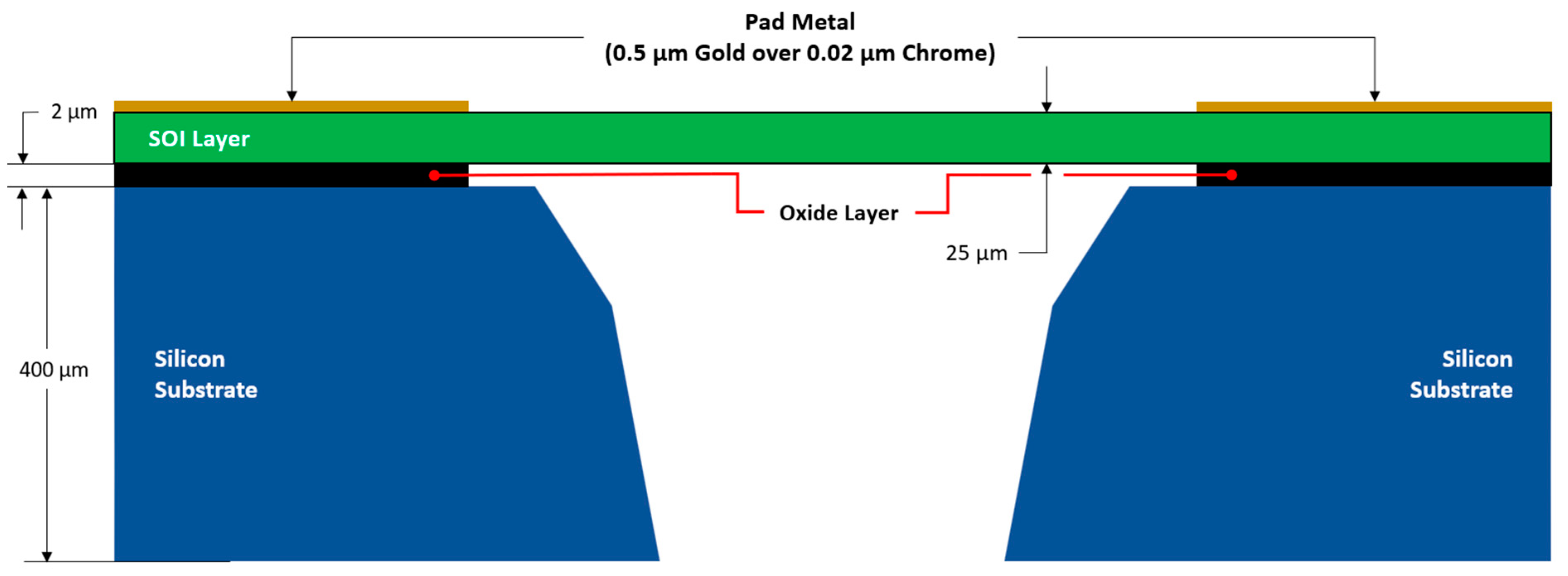
2. Fabrication Process Overview


3. Electrothermal MEMS Actuators’ Actuating Principles and Device Designs
3.1. MEMS Electrothermal Actuators’ Working Principles
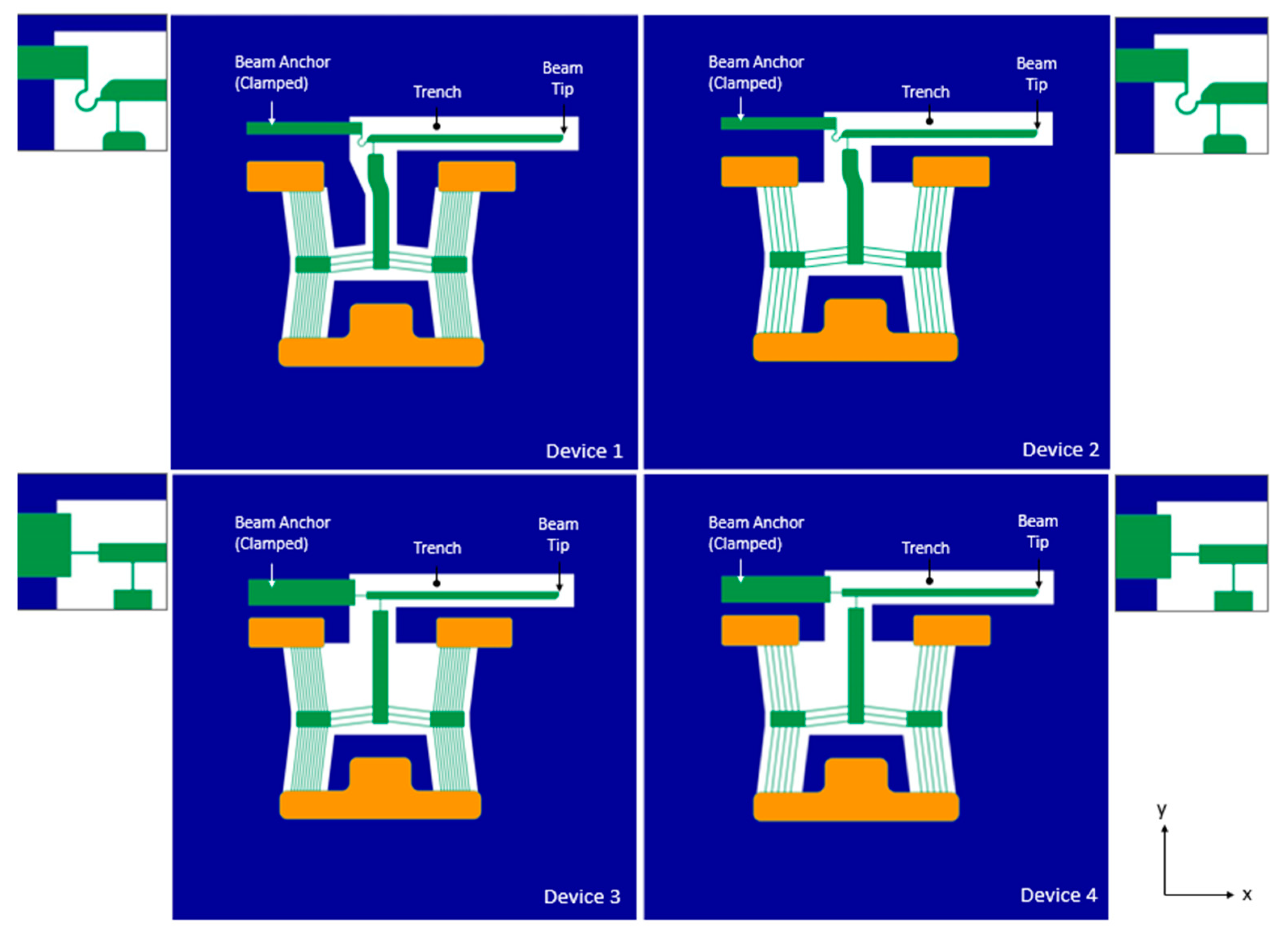
3.2. Device Designs and Configurations
4. Numerical Modelling
4.1. General
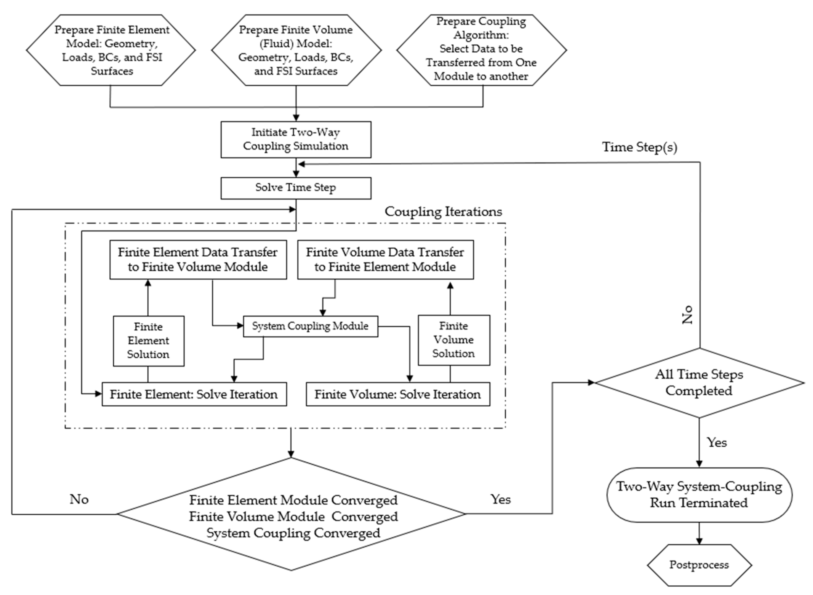
4.2. Thermo-Mechanical Fluid–Structure Interaction Numerical Modelling
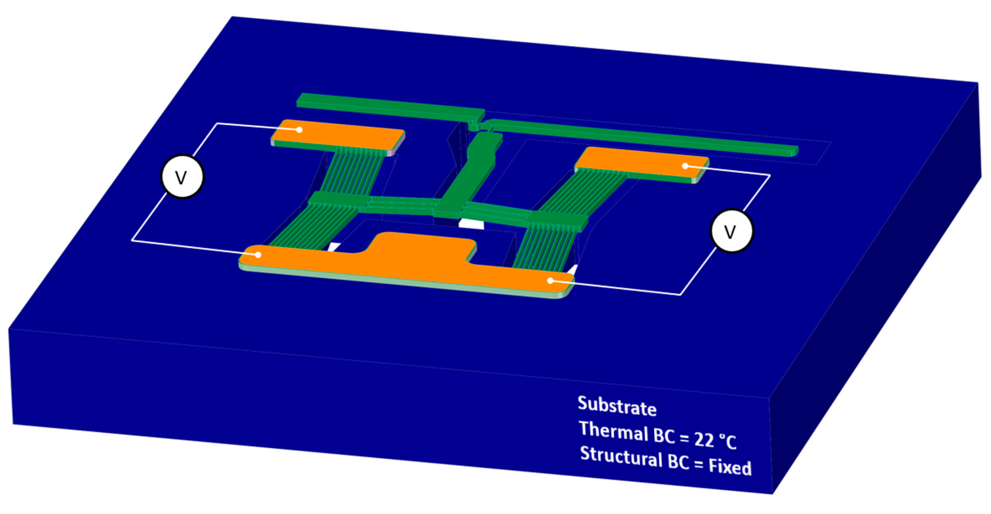
4.2.1. Finite Element Module—Model Setup
- i.
- A thermal boundary condition applied on the entire substrate as thermally clamped at 22 °C for all time steps;
- ii.
- The substrate was also mechanically clamped for all time steps, i.e., no translations are allowed;
- iii.
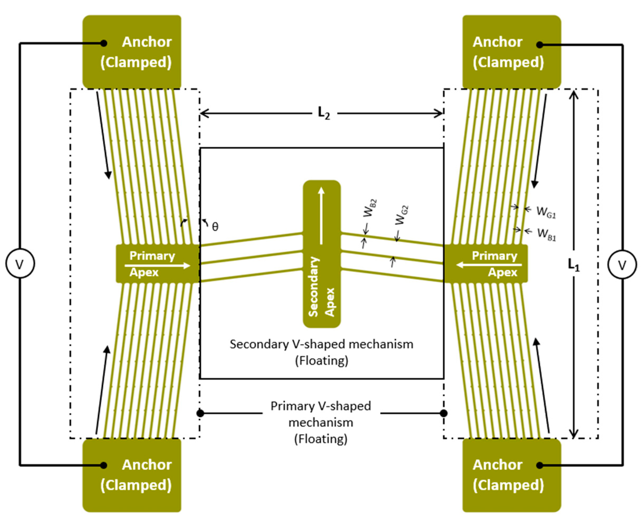
- A potential difference (V) was applied across the primary apexes via the pad metal regions, as denoted in Figure 6. The voltage loads for all devices were swept from 0 V to 5 V in increments of 1 V.

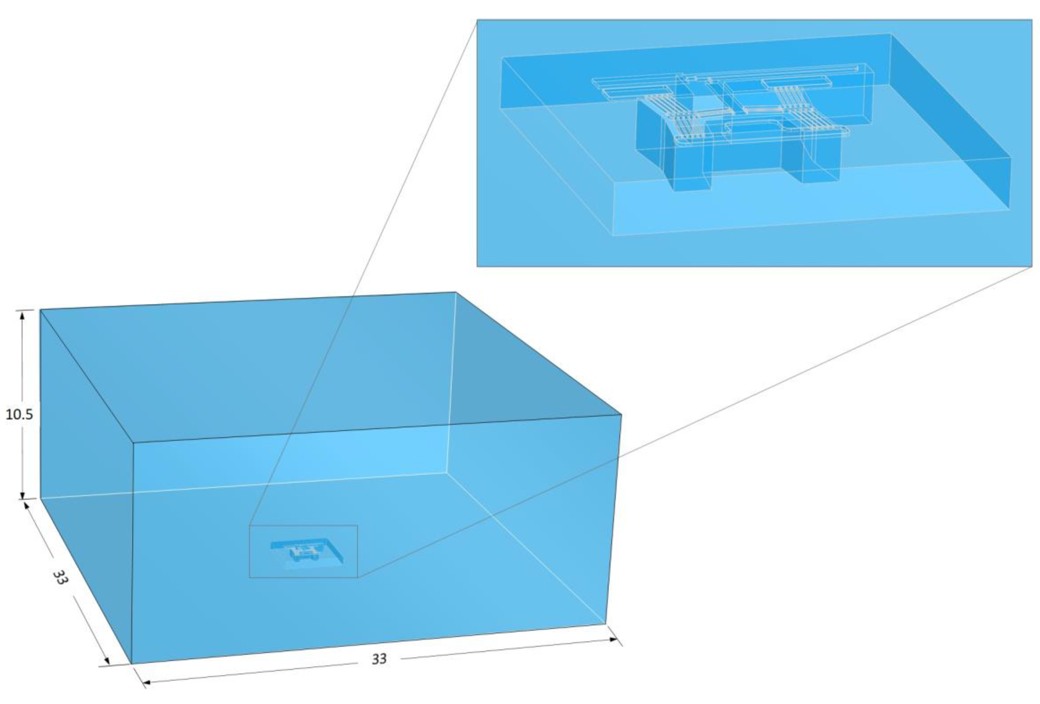
4.2.2. Finite Volume Module—Model Setup


- The bottom surface of the domain, which is assumed to be a fixed wall clamped at a constant temperature of 22 °C;
- The five extremities of the domain, which are assumed to be pressure outlets with a gauge pressure of 0 bar. Re-entry of the fluid is allowed here, with a temperature of 22 °C.
4.2.3. Data Transfer Setup
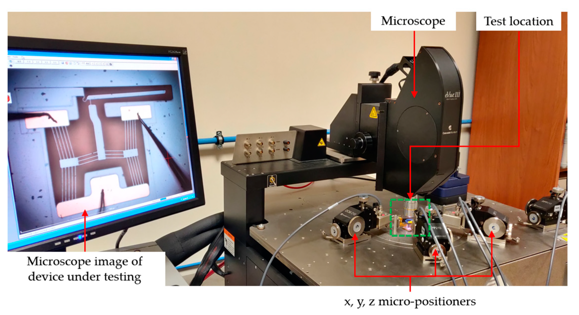
5. Experimental Testing
5.1. General
5.2. Testing in Air
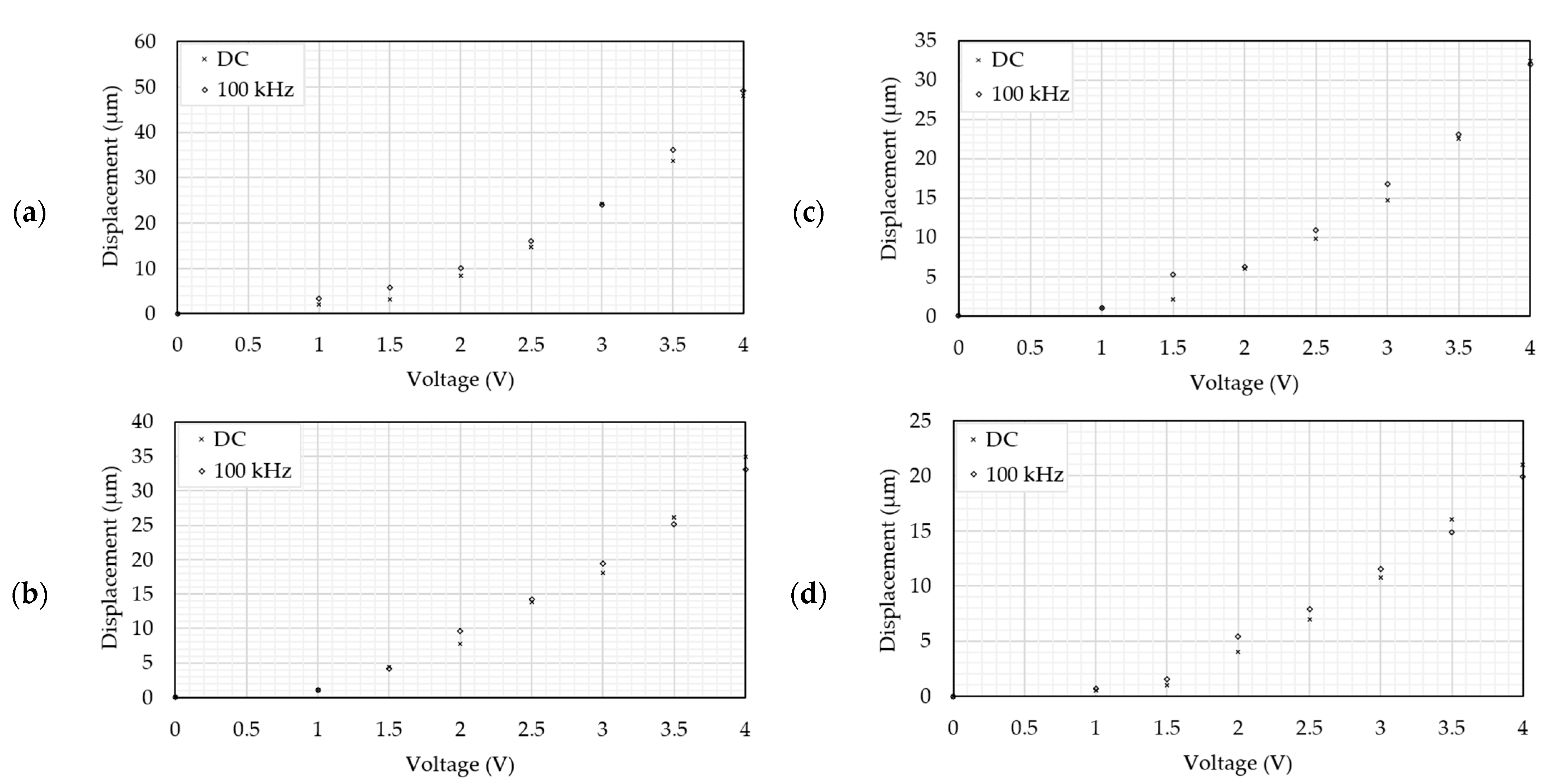
5.3. Frequency Independence Study
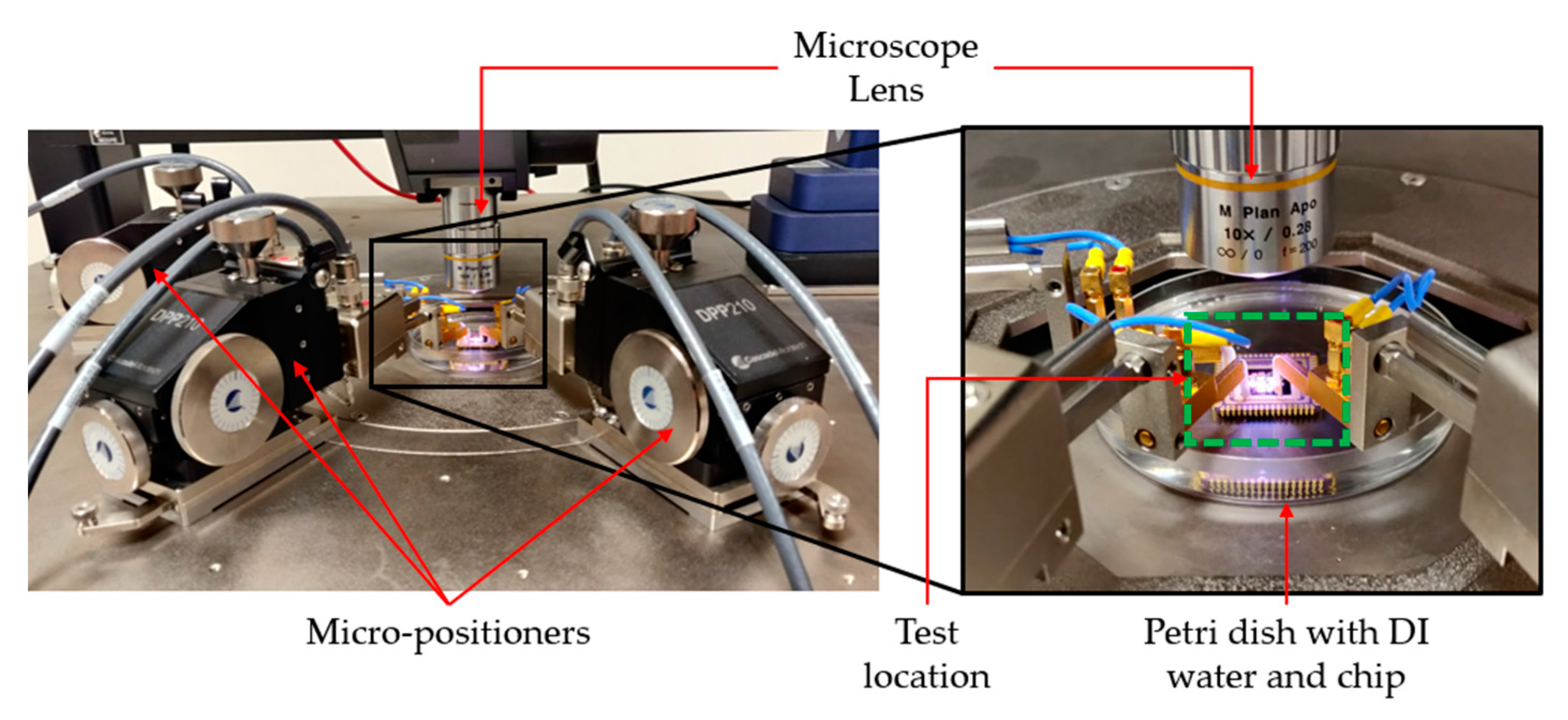
5.4. Testing in DI Water
- i.
- The devices were first subjected to a 10-minute soak in undiluted isopropyl alcohol (IPA);
- ii.
- The devices were then thoroughly rinsed three consecutive times in DI water;
- iii.
- Finally, the devices were submerged again in DI water for testing.
6. Results and Discussion
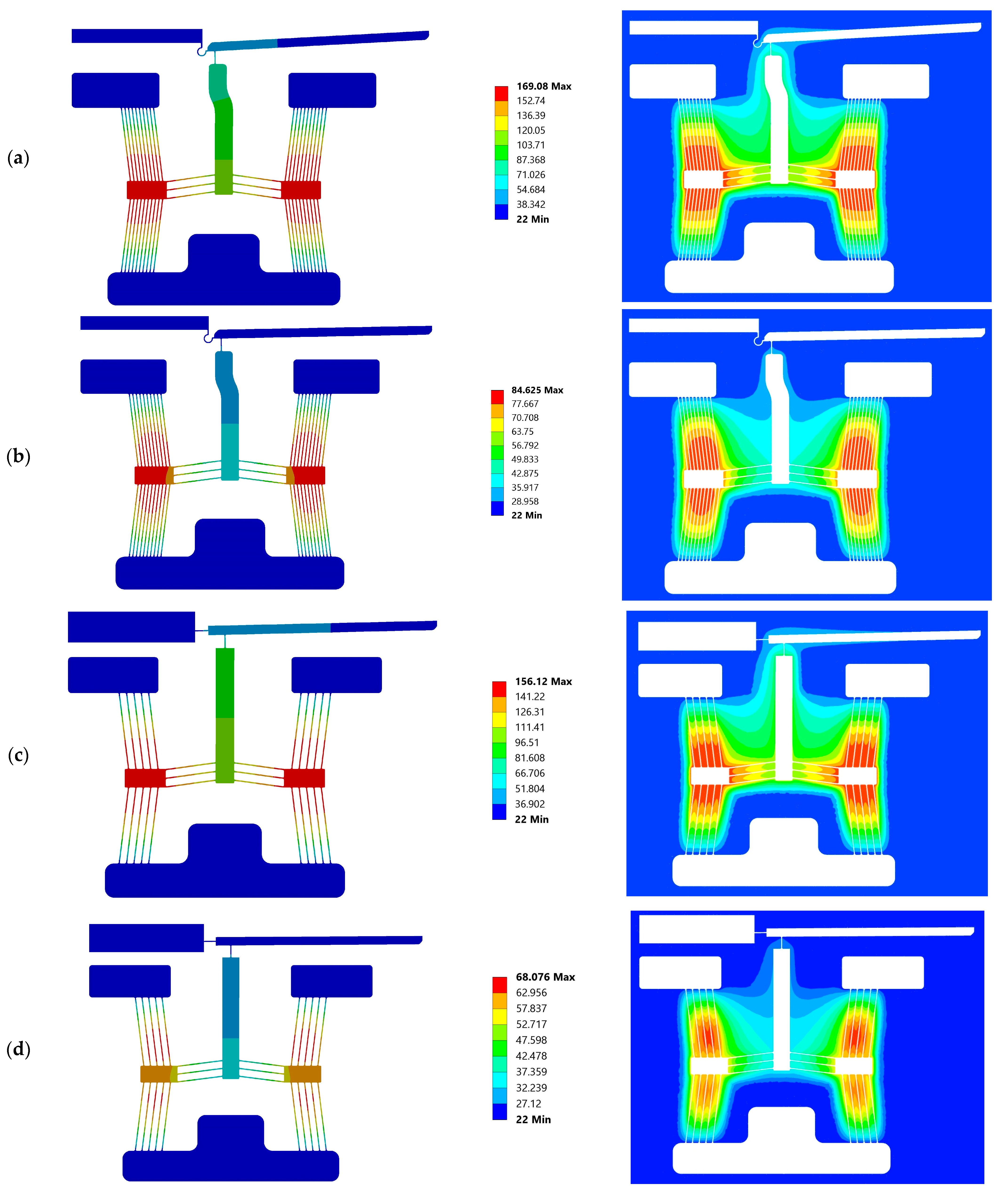
6.1. Electro-Thermal Performance
6.2. Structural Performance
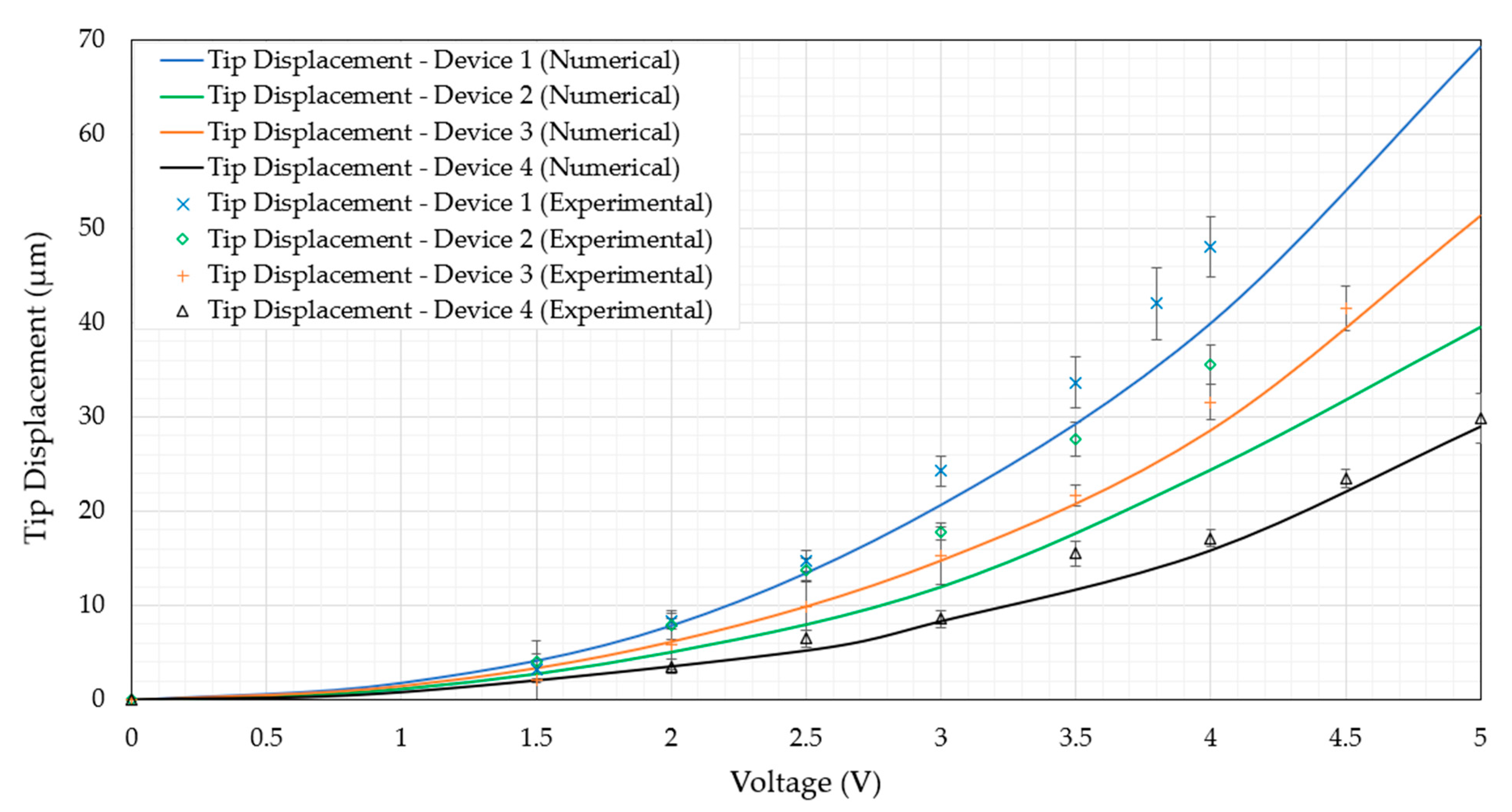
6.2.1. Device Structural Performance in Air
6.2.2. Frequency Independence Study in Air


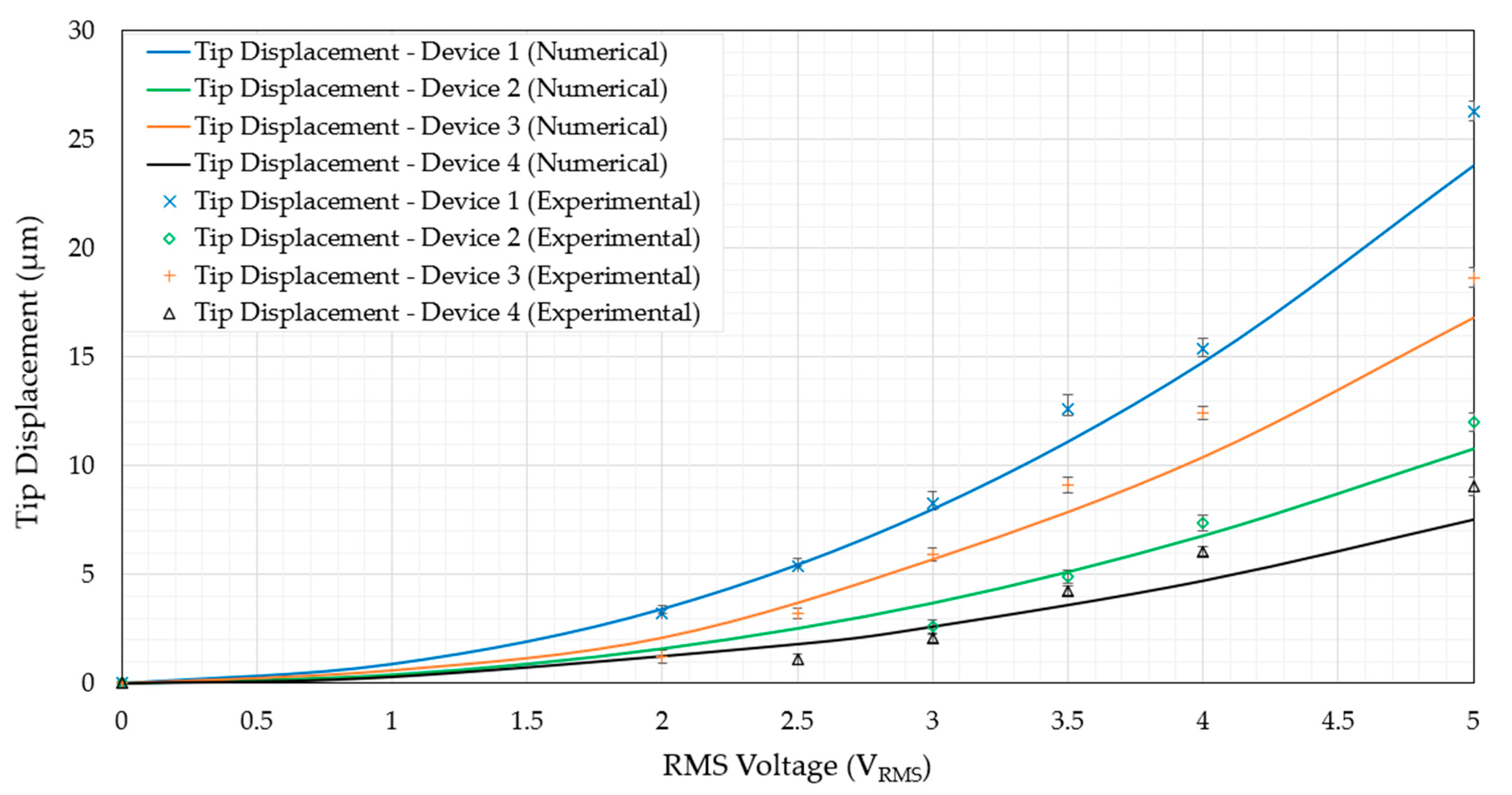
6.2.3. Device Structural Performance in DI Water
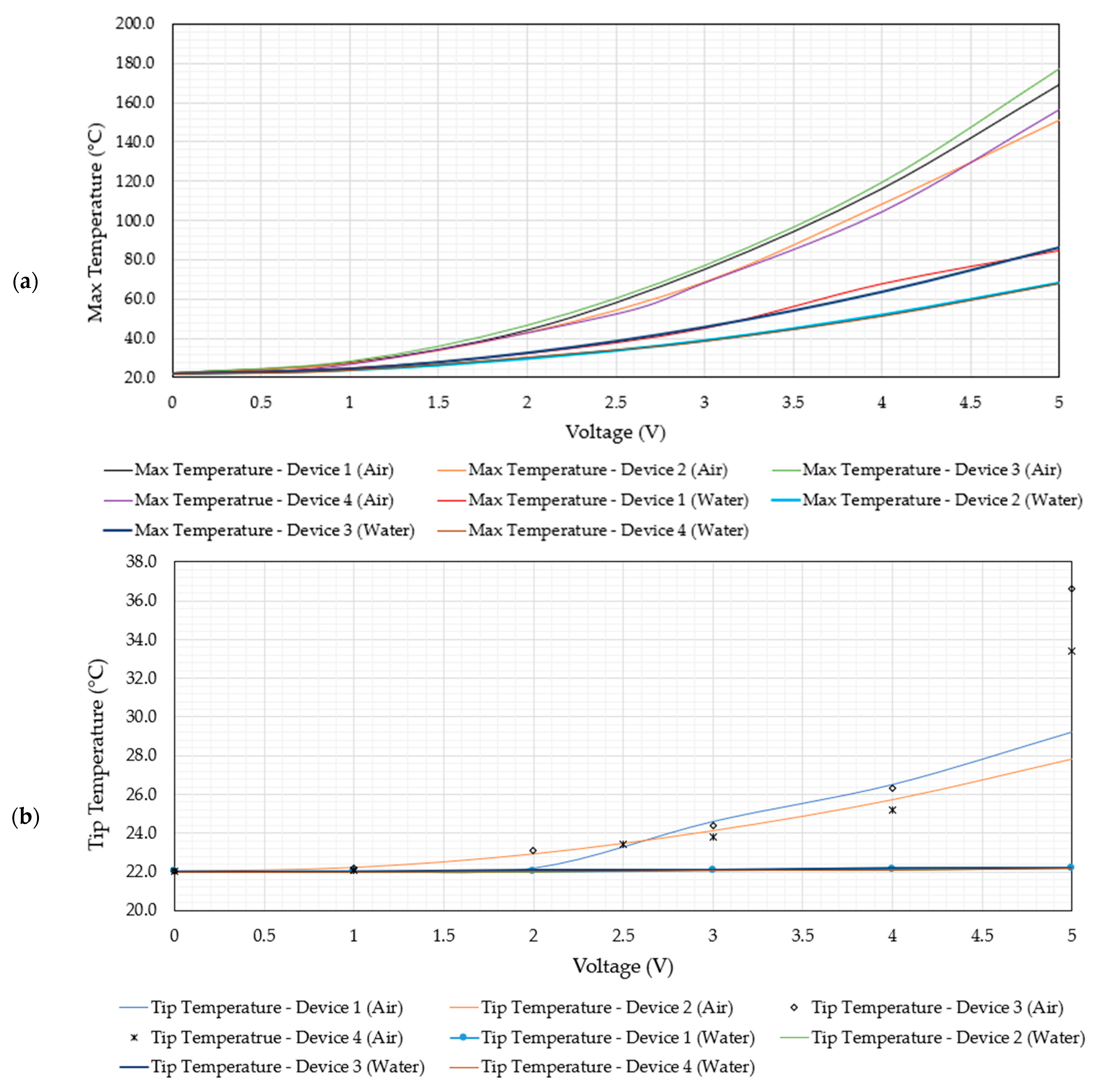
- All four devices operate at maximum temperatures well below 100 °C at an input voltage VRMS of 5 V;
- At VRMS = 5 V, all four devices maintain tip temperatures that are practically identical to the surrounding ambient temperature of 22 °C;
- The tip displacements at 5 V are all above 7 µm. The lowest was device 4, displaying experimental tip displacements of 9.1 µm, while the highest was showcased by device 1 at 26.3 µm.
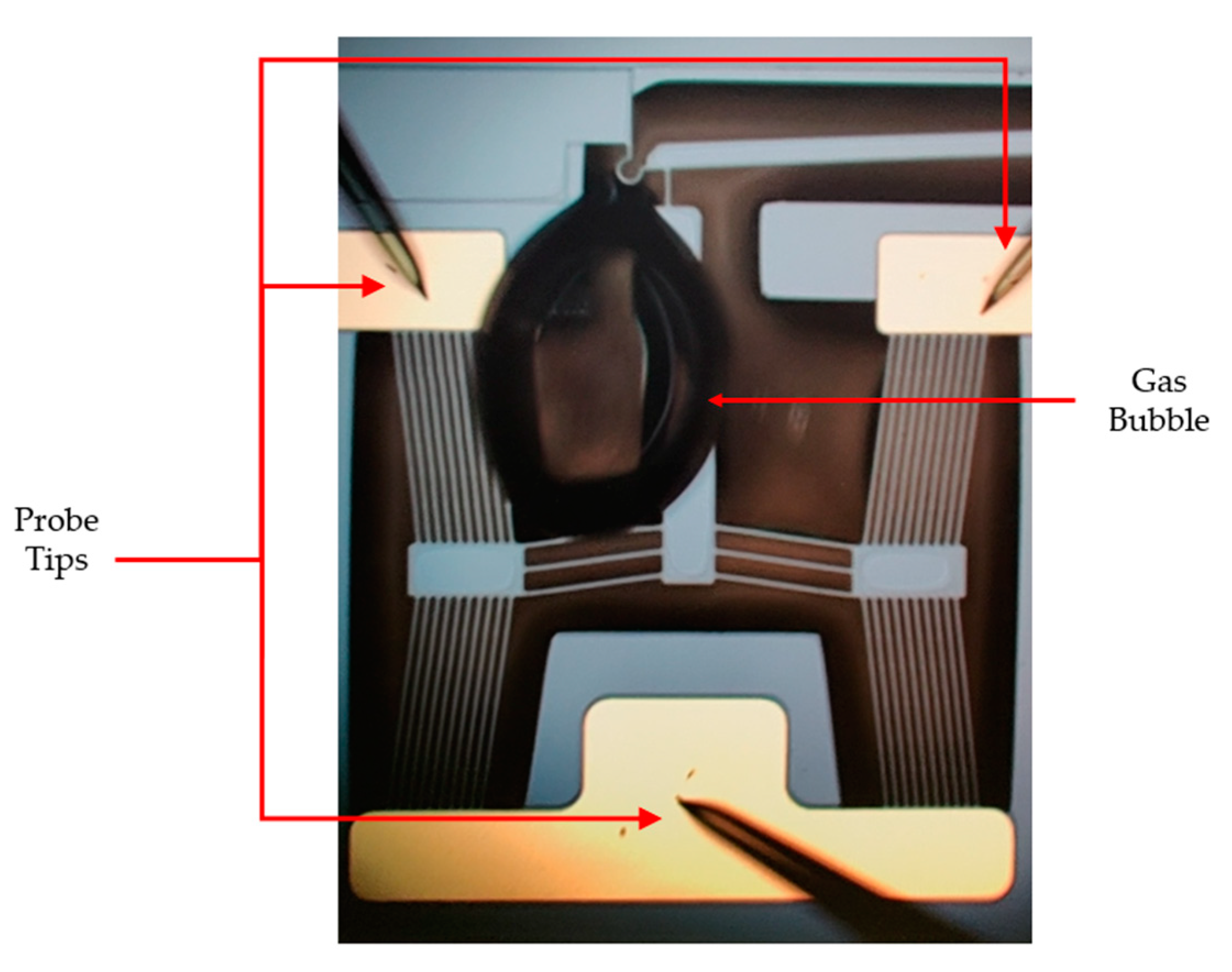
6.3. Gas Evolution Observation
7. Conclusions
Author Contributions
Funding
Data Availability Statement
Conflicts of Interest
Abbreviations
| BC | Boundary condition |
| ETA | Electrothermal actuator |
| FSI | Fluid–structure interaction |
| MEMS | Microelectromechanical system |
| SOI | Silicon-on-insulator |
| RBC | Red blood cell |
| DI | Deionised |
References
- Villarruel Mendoza, L.A.; Scilletta, N.A.; Bellino, M.G.; Desimone, M.F.; Catalano, P.N. Recent Advances in Micro-Electro-Mechanical Devices for Controlled Drug Release Applications. Front. Bioeng. Biotechnol. 2020, 8, 827. [Google Scholar] [CrossRef]
- Lee, H.J.; Choi, N.; Yoon, E.-S.; Cho, I.-J. MEMS devices for drug delivery. Adv. Drug Deliv. Rev. 2018, 128, 132–147. [Google Scholar] [CrossRef] [PubMed]
- Dong, X.; Johnson, W.; Sun, Y.; Liu, X. Robotic Micromanipulation of Cells and Small Organisms. In Micro- and Nanomanipulation Tools; John Wiley & Sons, Ltd.: Hoboken, NJ, USA, 2015; pp. 339–368. ISBN 9783527690237. [Google Scholar]
- Pan, P.; Wang, W.; Ru, C.; Sun, Y.; Liu, X. MEMS-based platforms for mechanical manipulation and characterization of cells. J. Micromech. Microeng. 2017, 27, 123003. [Google Scholar] [CrossRef]
- Belfiore, N.P.; Verotti, M.; Crescenzi, R.; Balucani, M. Design, optimization and construction of MEMS-based micro grippers for cell manipulation. In Proceedings of the 2013 International Conference on System Science and Engineering (ICSSE), Budapest, Hungary, 4–6 July 2013; pp. 105–110. [Google Scholar] [CrossRef]
- Cauchi, M.; Grech, I.; Mallia, B.; Mollicone, P.; Sammut, N. Analytical, Numerical and Experimental Study of a Horizontal Electrothermal MEMS Microgripper for the Deformability Characterisation of Human Red Blood Cells. Micromachines 2018, 9, 108. [Google Scholar] [CrossRef] [PubMed] [Green Version]
- Cauchi, M.; Grech, I.; Mallia, B.; Mollicone, P.; Sammut, N. The Effects of Cold Arm Width and Metal Deposition on the Performance of a U-Beam Electrothermal MEMS Microgripper for Biomedical Applications. Micromachines 2019, 10, 167. [Google Scholar] [CrossRef] [Green Version]
- Sciberras, T.; Demicoli, M.; Grech, I.; Mallia, B.; Mollicone, P.; Sammut, N. Experimental and Numerical Analysis of MEMS Electrothermal Actuators with Cascaded V-shaped Mechanisms. In Proceedings of the Design, Test, Integration & Packaging of MEMS/MOEMS, Pont-a-Mousson, France, 11–13 July 2022. [Google Scholar]
- Verotti, M.; Dochshanov, A.; Belfiore, N. A Comprehensive Survey on Modern Microgrippers Design: Mechanical Structure. J. Mech. Des. 2017, 139, 60801. [Google Scholar] [CrossRef]
- Dochshanov, A.; Verotti, M.; Belfiore, N. A Comprehensive Survey on Modern Microgrippers Design: Operational Strategy. J. Mech. Des. 2017, 139, 70801. [Google Scholar] [CrossRef]
- Cauchi, M.; Grech, I.; Mallia, B.; Mollicone, P.; Portelli, B.; Sammut, N. Essential design and fabrication considerations for the reliable performance of an electrothermal MEMS microgripper. Microsyst. Technol. 2019, 28, 1435–1450. [Google Scholar] [CrossRef]
- Liu, R.; Ye, X.; Cui, T. Recent Progress of Biomarker Detection Sensors. Research 2020, 2020, 7949037. [Google Scholar] [CrossRef]
- Nader, E.; Skinner, S.; Romana, M.; Fort, R.; Lemonne, N.; Guillot, N.; Gauthier, A.; Antoine-Jonville, S.; Renoux, C.; Hardy-Dessources, M.-D.; et al. Blood Rheology: Key Parameters, Impact on Blood Flow, Role in Sickle Cell Disease and Effects of Exercise. Front. Physiol. 2019, 10, 1329. [Google Scholar] [CrossRef] [Green Version]
- Musielak, M. Red blood cell-deformability measurement: Review of techniques. Clin. Hemorheol. Microcirc. 2009, 42, 47–64. [Google Scholar] [CrossRef] [PubMed]
- Parrow, N.L.; Violet, P.-C.; Tu, H.; Nichols, J.; Pittman, C.A.; Fitzhugh, C.; Fleming, R.E.; Mohandas, N.; Tisdale, J.F.; Levine, M. Measuring Deformability and Red Cell Heterogeneity in Blood by Ektacytometry. J. Vis. Exp. 2018, 131, e56910. [Google Scholar] [CrossRef]
- Chen, X.; Feng, L.; Jin, H.; Feng, S.; Yu, Y. Quantification of the erythrocyte deformability using atomic force microscopy: Correlation study of the erythrocyte deformability with atomic force microscopy and hemorheology. Clin. Hemorheol. Microcirc. 2009, 43, 243–251. [Google Scholar] [CrossRef] [PubMed]
- Jaiswal, D.; Cowley, N.; Bian, Z.; Zheng, G.; Claffey, K.P.; Hoshino, K. Stiffness analysis of 3D spheroids using microtweezers. PLoS ONE 2017, 12, e0188346. [Google Scholar] [CrossRef] [Green Version]
- Mills, J.P.; Qie, L.; Dao, M.; Lim, C.T.; Suresh, S. Nonlinear elastic and viscoelastic deformation of the human red blood cell with optical tweezers. Mech. Chem. Biosyst. 2004, 1, 169–180. [Google Scholar]
- Kuzman, D.; Svetina, S.; Waugh, R.E.; Zeks, B. Elastic properties of the red blood cell membrane that determine echinocyte deformability. Eur. Biophys. J. 2004, 33, 1–15. [Google Scholar] [CrossRef]
- Gnerlich, M.; Perry, S.F.; Tatic-Lucic, S. A submersible piezoresistive MEMS lateral force sensor for a diagnostic biomechanics platform. Sensors Actuators A Phys. 2012, 188, 111–119. [Google Scholar] [CrossRef]
- Potter, R.F.; Groom, A.C. Capillary diameter and geometry in cardiac and skeletal muscle studied by means of corrosion casts. Microvasc. Res. 1983, 25, 68–84. [Google Scholar] [CrossRef]
- Lecklin, T.; Egginton, S.; Nash, G.B. Effect of temperature on the resistance of individual red blood cells to flow through capillary-sized apertures. Pflugers Arch. 1996, 432, 753–759. [Google Scholar] [CrossRef]
- Fildes, J.; Fisher, S.; Sheaff, C.M.; Barrett, J.A. Effects of Short Heat Exposure on Human Red and White Blood Cells. J. Trauma Acute Care Surg. 1998, 45, 479–484. [Google Scholar] [CrossRef]
- Singh, M.; Stoltz, J. Influence of temperature variation from 5 °C to 37 °C on aggregation and deformability of erythrocytes. Clin. Hemorheol. Microcirc. 2002, 26, 1–7. [Google Scholar] [PubMed]
- Lukose, J.; Shastry, S.; Mithun, N.; Mohan, G.; Ahmed, A.; Chidangil, S. Red blood cells under varying extracellular tonicity conditions: An optical tweezers combined with micro-Raman study. Biomed. Phys. Eng. express 2020, 6, 15036. [Google Scholar] [CrossRef]
- Lopez, M.J.; Hall, C.A. Physiology, Osmosis. Available online: https://www.ncbi.nlm.nih.gov/books/NBK557609/ (accessed on 28 February 2023).
- Moritz, M.L. Why 0.9% saline is isotonic: Understanding the aqueous phase of plasma and the difference between osmolarity and osmolality. Pediatr. Nephrol. 2019, 34, 1299–1300. [Google Scholar] [CrossRef] [PubMed]
- Zhang, W.; Gnerlich, M.; Paly, J.; Sun, Y.; Jing, G.; Voloshin, A.; Tatic-Lucic, S. A polymer V-shaped electrothermal actuator array for biological applications. J. Micromech. Microeng. 2008, 18, 75020. [Google Scholar] [CrossRef]
- Xu, Z.; Zheng, Y.; Wang, X.; Shehata, N.; Wang, C.; Sun, Y. Stiffness increase of red blood cells during storage. Microsyst. Nanoeng. 2018, 4, 17103. [Google Scholar] [CrossRef] [Green Version]
- Barshtein, G.; Pajic-Lijakovic, I.; Gural, A. Deformability of Stored Red Blood Cells. Front. Physiol. 2021, 12, 722896. [Google Scholar] [CrossRef]
- Sameoto, D.; Hubbard, T.; Kujath, M. Operation of electrothermal and electrostatic MUMPs microactuators underwater. J. Micromech. Microeng. 2004, 14, 1359. [Google Scholar] [CrossRef]
- Mukundan, V.; Ponce, P.; Butterfield, H.E.; Pruitt, B.L. Modeling and Characterization of Electrostatic Comb-drive Actuators in Conducting Liquid Media. J. Micromech. Microeng. 2009, 19, 065008. [Google Scholar] [CrossRef] [Green Version]
- Hon, M.; DelRio, F.W.; White, J.T.; Kendig, M.; Carraro, C.; Maboudian, R. Cathodic corrosion of polycrystalline silicon MEMS. Sensors Actuators A Phys. 2008, 145–146, 323–329. [Google Scholar] [CrossRef]
- Zumdahl, S.S. Chemical Principles; D.C. Heath and Company: Lexington, MA, USA, 1992; ISBN 9780669278712. [Google Scholar]
- Cowen, A.; Hames, G.; Monk, D.; Wilcenski, S.; Hardy, B. SOIMUMPs Design Handbook; Memscap Inc.: Durham, NC, USA, 2011; Volume 6. [Google Scholar]
- Potekhina; Wang Review of Electrothermal Actuators and Applications. Actuators 2019, 8, 69. [CrossRef] [Green Version]
- Sciberras, T.; Demicoli, M.; Grech, I.; Mallia, B.; Mollicone, P.; Sammut, N. Coupled Finite Element-Finite Volume Multi-Physics Analysis of MEMS Electrothermal Actuators. Micromachines 2022, 13, 8. [Google Scholar] [CrossRef]
- Que, L.; Park, J.; Gianchandani, Y.B. Bent-beam electrothermal actuators-Part I: Single beam and cascaded devices. Microelectromech. Syst. J. 2001, 10, 247–254. [Google Scholar] [CrossRef] [Green Version]
- Cauchi, M.; Grech, I.; Mallia, B.; Mollicone, P.; Sammut, N. The Effects of Structure Thickness, Air Gap Thickness and Silicon Type on the Performance of a Horizontal Electrothermal MEMS Microgripper. Actuators 2018, 7, 38. [Google Scholar] [CrossRef] [Green Version]
- Voicu, R. An SU-8 Microgripper Based on the Cascaded V-Shaped Electrothermal Actuators: Design, Fabrication, Simulation and Experimental Investigations; IntechOpen: Rijeka, Croatia, 2018. [Google Scholar] [CrossRef]
- Shen, X.; Chen, X. Mechanical Performance of a Cascaded V-Shaped Electrothermal Actuator. Int. J. Adv. Robot. Syst. 2013, 10, 379. [Google Scholar] [CrossRef]
- Voicu, R.-C. Design, numerical simulation and experimental investigation of an {SU}-8 microgripper based on the cascaded V-shaped electrothermal actuators. J. Phys. Conf. Ser. 2016, 757, 12015. [Google Scholar] [CrossRef] [Green Version]
- Hickey, R.; Sameoto, D.; Hubbard, T.; Kujath, M. Time and frequency response of two-arm micromachined thermal actuators. J. Micromech. Microeng. 2002, 13, 40–46. [Google Scholar] [CrossRef]
- Qu, J.; Zhang, W.; Jung, A.; Silva-Da Cruz, S.; Liu, X. Microscale Compression and Shear Testing of Soft Materials Using an MEMS Microgripper With Two-Axis Actuators and Force Sensors. IEEE Trans. Autom. Sci. Eng. 2017, 14, 834–843. [Google Scholar] [CrossRef]
- Krecinic, F.; Duc, T.C.; Lau, G.K.; Sarro, P.M. Finite element modelling and experimental characterization of an electro-thermally actuated silicon-polymer micro gripper. J. Micromech. Microeng. 2008, 18, 64007. [Google Scholar] [CrossRef]
- Thangavel, A.; Rengaswamy, R.; Sukumar, P.K.; Sekar, R. Modelling of Chevron electrothermal actuator and its performance analysis. Microsyst. Technol. 2018, 24, 1767–1774. [Google Scholar] [CrossRef]
- Nilesh D Mankame; G K Ananthasuresh Comprehensive thermal modelling and characterization of an electro-thermal-compliant microactuator. J. Micromech. Microeng. 2001, 11, 452. [CrossRef]
- Serrano, J.R.; Phinney, L.M.; Rogers, J.W. Temperature amplification during laser heating of polycrystalline silicon microcantilevers due to temperature-dependent optical properties. Int. J. Heat Mass Transf. 2009, 52, 2255–2264. [Google Scholar] [CrossRef]
- Bharali, A.K.; Patowari, P.K.; Baishya, S. Design and analysis of multilayer electrothermal actuator for MEMS. In Proceedings of the 2010 2nd International Conference on Mechanical and Electronics Engineering, Kyoto, Japan, 1–3 August 2010; Volume 1, pp. V1-127–V1-131. [Google Scholar] [CrossRef]
- Yallew, T.S.; Pantano, M.F.; Bagolini, A. Design and Finite Element Analysis of an Electrothermally Actuated Microgripper for Biomedical Applications. In Proceedings of the 2021 Symposium on Design, Test, Integration & Packaging of MEMS and MOEMS (DTIP), Paris, France, 25–27 August 2021; pp. 1–5. [Google Scholar] [CrossRef]
- Liu, T.; Pan, T.; Qin, S.; Zhao, H.; Xie, H. Dynamic Response Analysis of an Immersed Electrothermally Actuated MEMS Mirror. Actuators 2023, 12, 83. [Google Scholar] [CrossRef]
- ANSYS. Academic Research Mechanical, Release 18.2, Help System, Mechanical APDL Theory Reference; ANSYS, Inc.: Canonsburg, PA, USA; Available online: https://www.ansys.com/legal/terms-and-conditions (accessed on 28 February 2023).
- ANSYS. Academic Research Mechanical, Release 21.1, Help System, ANSYS Fluent Theory Guide; ANSYS, Inc.: Canonsburg, PA, USA; Available online: https://www.ansys.com/legal/terms-and-conditions (accessed on 28 February 2023).
- Incropera, F.P.; DeWitt, D.P. Fundamentals of Heat and Mass Transfer, 4th ed.; John Wiley & Sons, Inc.: New York, NY, USA, 1996. [Google Scholar]
- ANSYS. Academic Research Mechanical, Release 15.0, Help System, ANSYS Fluent User’s Guide; ANSYS, Inc.: Canonsburg, PA, USA; Available online: https://www.ansys.com/legal/terms-and-conditions (accessed on 28 February 2023).


| Property Designation | SOI | Pad Metal |
|---|---|---|
| Shear modulus, G [GPa] | Gyz = Gzx = 79.6, Gxy = 50.9 | N/A |
| Young’s modulus, E [GPa] | Ex = Ey = 169, Ez = 130 | 57 |
| Poisson’s ratio, ν | νyz = 0.36, νzx = 0.29, νxy = 0.064 | 0.35 |
| Thermal conductivity, k [W/m·K] | 148 | 297 |
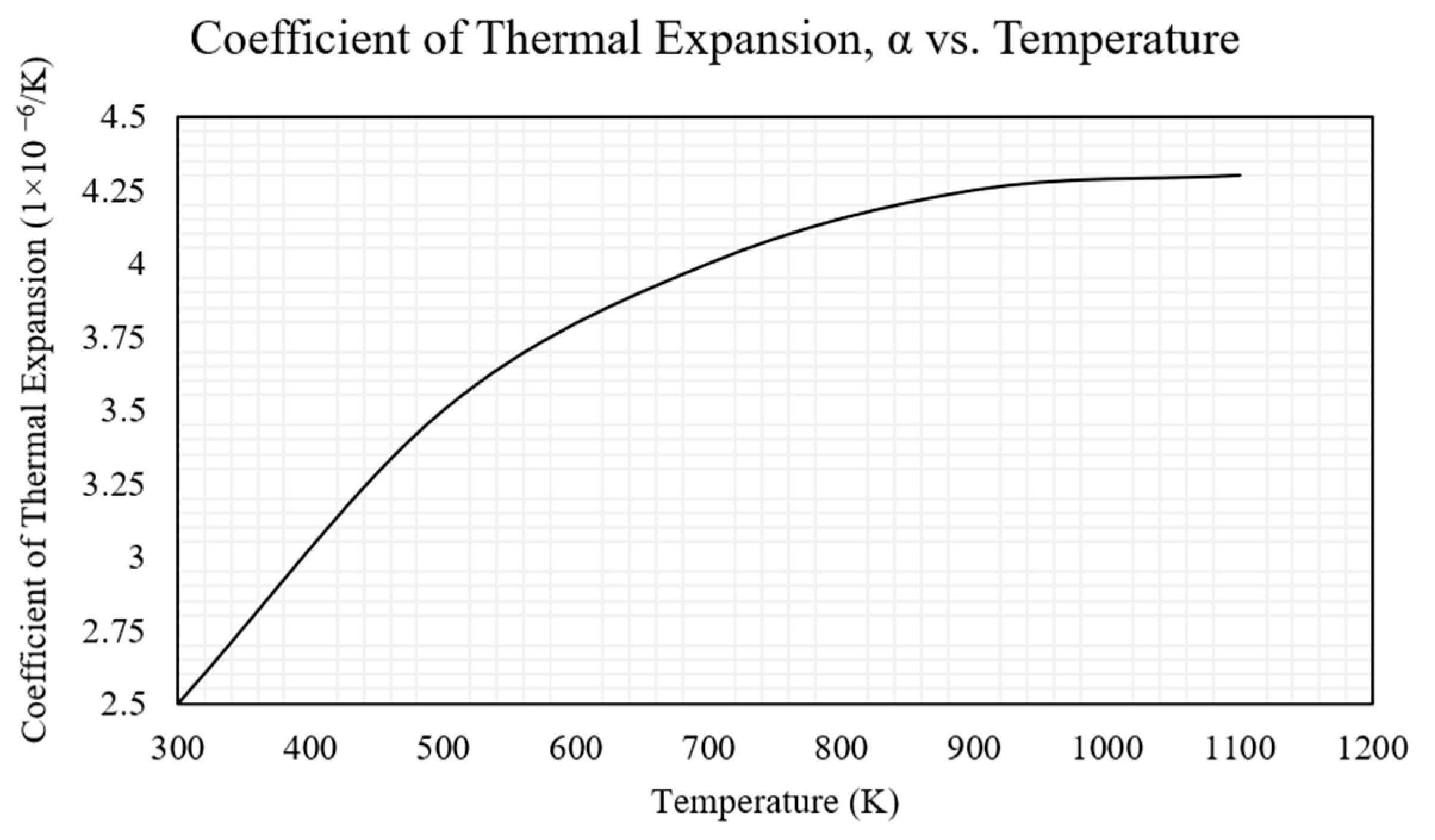
| Coefficient of thermal expansion, α [µm/m·K] | Refer to Figure 2 | N/A |
| Density [g/(cm)3] | 2.50 | 19.30 |
| Specific heat capacity, c [J/kg·K] | 712 | 128.7 |
| Electrical resistivity, ρ [µ·Ω·m] | 125 | 2.86 × 10⁻² |
| Variable | Value | |||
|---|---|---|---|---|
| Device 1 | Device 2 | Device 3 | Device 4 | |
| Number of beams per side (primary V-shaped mechanism) | 10 | 5 | 10 | 5 |
| Number of beams per side (secondary V-shaped mechanism) | 3 | 3 | 3 | 3 |
| Primary beam width, wB1 (µm) | 6 | 6 | 6 | 6 |
| Primary beam spacing, wG1 (µm) | 14 | 34 | 14 | 34 |
| Secondary beam width, wB2 (µm) | 6.6 | 6.6 | 6.6 | 6.6 |
| Secondary beam spacing, wG2 (µm) | 40 | 40 | 40 | 40 |
| Distance between anchors of primary V-shaped mechanism, L1 (µm) | 920 | 920 | 920 | 920 |
| Distance between primary apexes (at rest and 22 °C), L2 (µm) | 640 | 640 | 640 | 640 |
| Pre-bend angle, θ (°) | 7 | 7 | 7 | 7 |
| Property | Fluid | |
|---|---|---|
| Air | Water | |
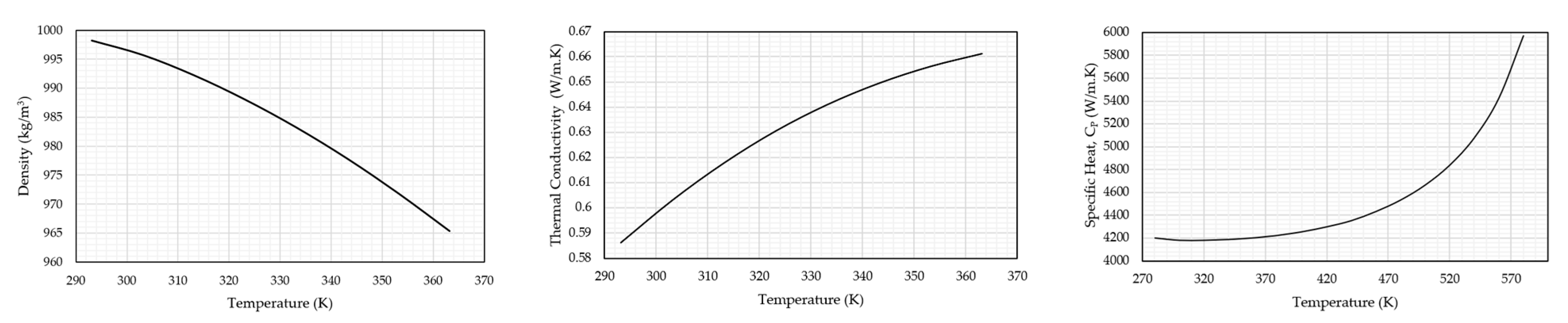
| Density | Refer to Equation (2) | Refer to Figure 8 |
| Specific heat at constant pressure, J/kg·K | 1006.43 | |
| Thermal Conductivity, W/(m·K) | 0.02602 | |
| Viscosity, kg/(m·s) | 1.7894 × 10⁻⁴ | 10.03 × 10⁻⁴ |
| Molecular weight, kg/kmol | 28.966 | N/A |
| Data Source | Target Module | Source Variable | Affected Target Variable | Thermal Coupling [37] | Thermo- Mechanical Coupling |
|---|---|---|---|---|---|
| Finite Volume | Finite Element | Heat Transfer Coefficient | Convection Coefficient | ✓ | ✓ |
| Finite Volume | Finite Element | Near Wall Temperature | Convection Reference Temperature | ✓ | ✓ |
| Finite Element | Finite Volume | Temperature | Temperature | ✓ | ✓ |
| Finite Volume | Finite Element | Force | Force | N/A | ✓ |
| Finite Element | Finite Volume | Incremental Displacement | Displacement | N/A | ✓ |
| Device/s | Voltage Range |
|---|---|
| 1 and 2 | 0 V–4 V |
| 3 | 0 V–4.5 V |
| 4 | 0 V–5 V |
| Voltage (V) | Percentage Difference (%) | |||||||
|---|---|---|---|---|---|---|---|---|
| Tip | Maximum | |||||||
| Device 1 | Device 2 | Device 3 | Device 4 | Device 1 | Device 2 | Device 3 | Device 4 | |
| 0 | 0 | 0 | 0 | 0 | 0 | 0 | 0 | 0 |
| 1 | 0.14 | 0.9 | 0.9 | 0.45 | 10.40 | 12.18 | 13.33 | 12.18 |
| 2 | 0.90 | 4.01 | 4.42 | / | 31.36 | 35.68 | 34.94 | / |
| 2.5 | / | / | / | 5.94 | / | / | / | 41.94 |
| 3 | 10.84 | 8.66 | 9.89 | 7.41 | 50.23 | 55.22 | 50.90 | 55.33 |
| 4 | 17.88 | 15.06 | 16.91 | 13.11 | 52.72 | 70.42 | 60.98 | 67.95 |
| 5 | 27.24 | 27.8 | 48.98 | 40.29 | 66.61 | 75.62 | 69.20 | 78.51 |
| Voltage | Percentage (%) | |||
|---|---|---|---|---|
| Device 1 | Device 2 | Device 3 | Device 4 | |
| 2 | 38.50 | N/A | 20.76 | N/A |
| 2.5 | 36.54 | N/A | 32.42 | 17.00 |
| 3 | 34.12 | 14.63 | 38.69 | 24.24 |
| 3.5 | 37.44 | 17.62 | 42.00 | 27.52 |
| 4.0 | 32.00 | 20.69 | 39.30 | 35.53 |
Disclaimer/Publisher’s Note: The statements, opinions and data contained in all publications are solely those of the individual author(s) and contributor(s) and not of MDPI and/or the editor(s). MDPI and/or the editor(s) disclaim responsibility for any injury to people or property resulting from any ideas, methods, instructions or products referred to in the content. |
© 2023 by the authors. Licensee MDPI, Basel, Switzerland. This article is an open access article distributed under the terms and conditions of the Creative Commons Attribution (CC BY) license (https://creativecommons.org/licenses/by/4.0/).
Share and Cite
Sciberras, T.; Demicoli, M.; Grech, I.; Mallia, B.; Mollicone, P.; Sammut, N. Thermo-Mechanical Fluid–Structure Interaction Numerical Modelling and Experimental Validation of MEMS Electrothermal Actuators for Aqueous Biomedical Applications. Micromachines 2023, 14, 1264. https://doi.org/10.3390/mi14061264
Sciberras T, Demicoli M, Grech I, Mallia B, Mollicone P, Sammut N. Thermo-Mechanical Fluid–Structure Interaction Numerical Modelling and Experimental Validation of MEMS Electrothermal Actuators for Aqueous Biomedical Applications. Micromachines. 2023; 14(6):1264. https://doi.org/10.3390/mi14061264
Chicago/Turabian StyleSciberras, Thomas, Marija Demicoli, Ivan Grech, Bertram Mallia, Pierluigi Mollicone, and Nicholas Sammut. 2023. "Thermo-Mechanical Fluid–Structure Interaction Numerical Modelling and Experimental Validation of MEMS Electrothermal Actuators for Aqueous Biomedical Applications" Micromachines 14, no. 6: 1264. https://doi.org/10.3390/mi14061264