
Kinematic Properties of a Twisted Double Planetary Chaotic Mixer: A Three-Dimensional Numerical Investigation
 ,
,  ,
, 
Abstract
:1. Introduction
2. Geometrical Description and Modeling
3. Mesh Study
4. Results and Discussion
4.1. Flow Characteristics
4.2. Poincaré Map
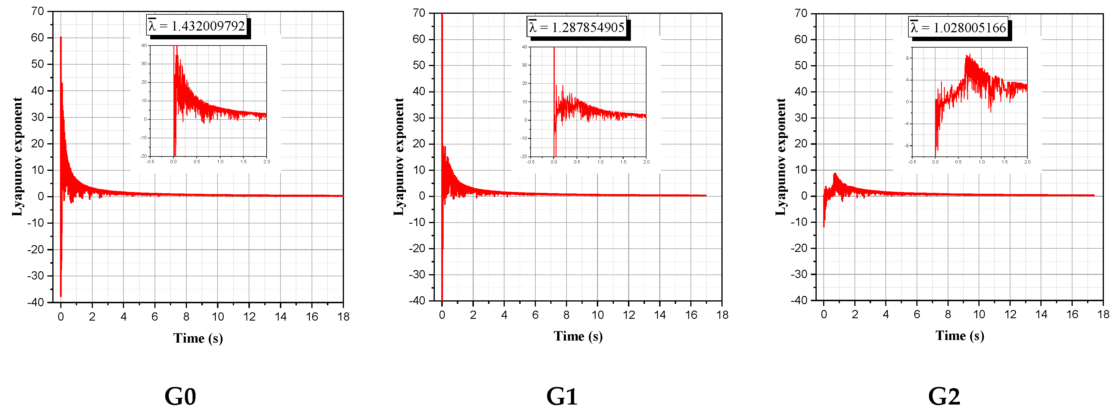
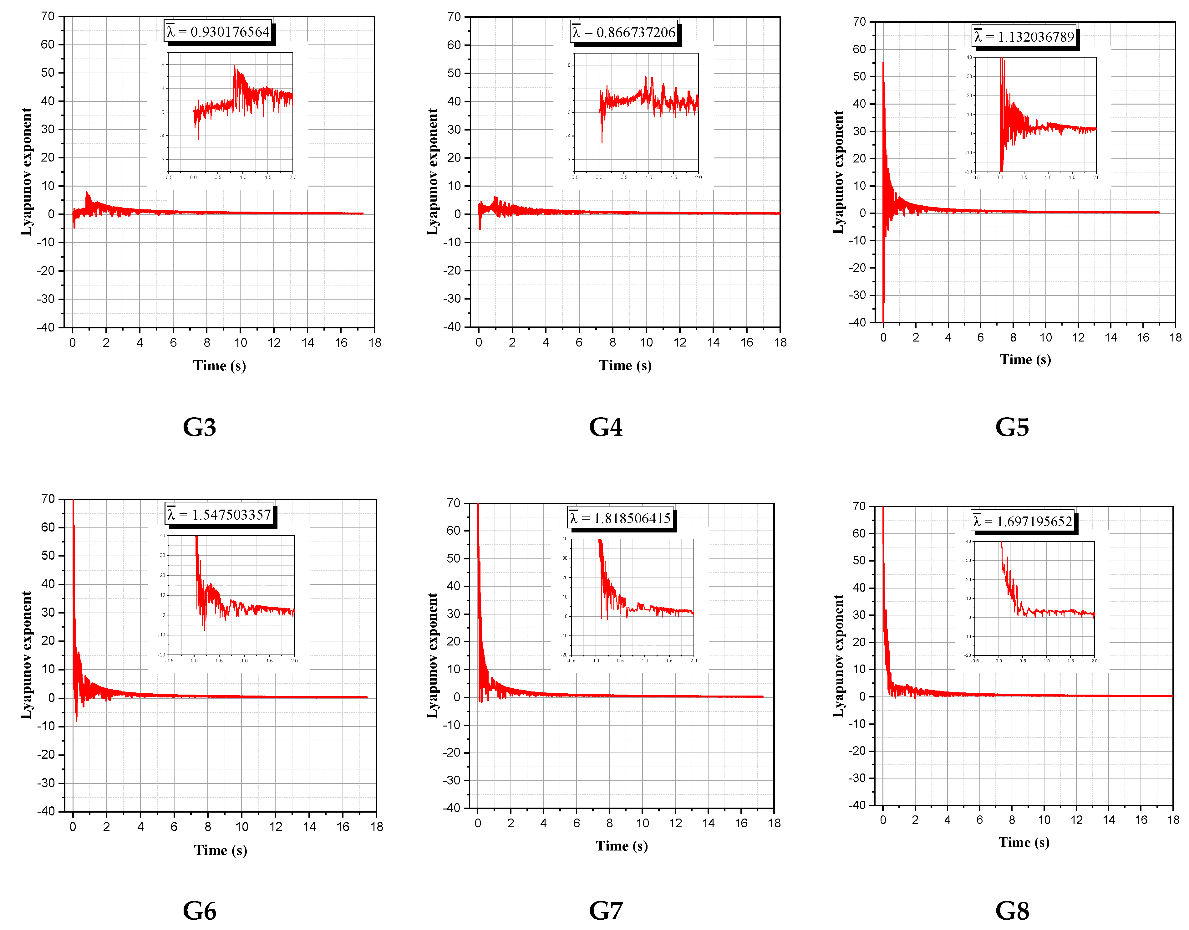
4.3. Lyapunov Exponent
4.4. Kinematic Properties
- a.
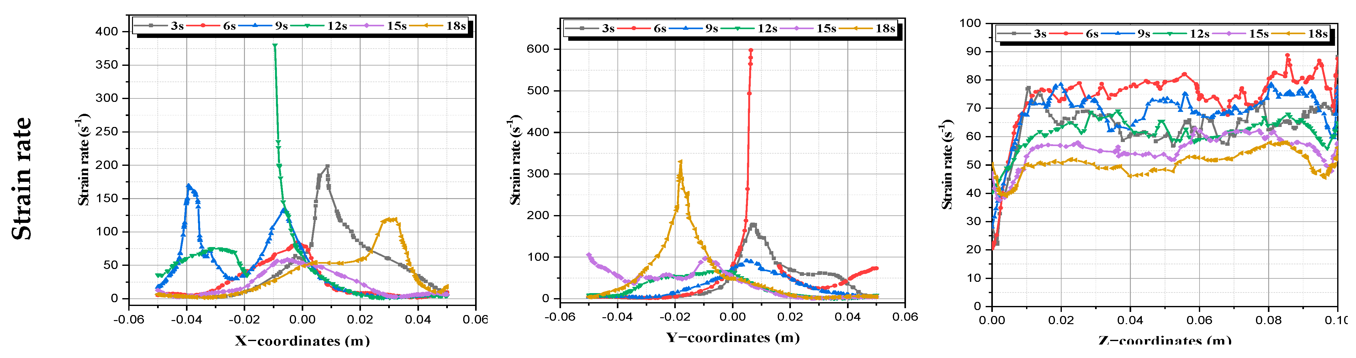
- Strain rate (deformation): It represents the change in the strain of a specific material over time. It is expressed by the following expression [46]:
- b.
- c.
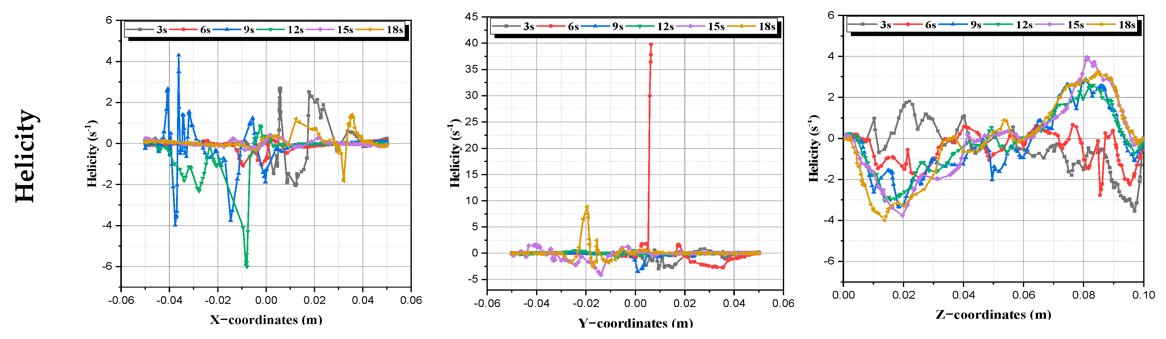
- Helicity: It is simply the projection of a spin vector in the orientation of its momentum vector. Helicity is positive if the particle spin vector points and the momentum vector take the same direction, and it will be negative if the point is in the opposite direction. We see in Figure 11 that this property can take both positive and negative values, as it spreads throughout the flow domain; note that this property takes large values near the agitating rods [46].
- d.
- Elongation rate: Itis defined as the compression or the extension of fluid particle, i.e., it can take either negative or positive values. The generalized elongation rate ε can be expressed by the following Equation (12), which is calculated from the analytical derivatives of the velocity components, as follows.
- e.
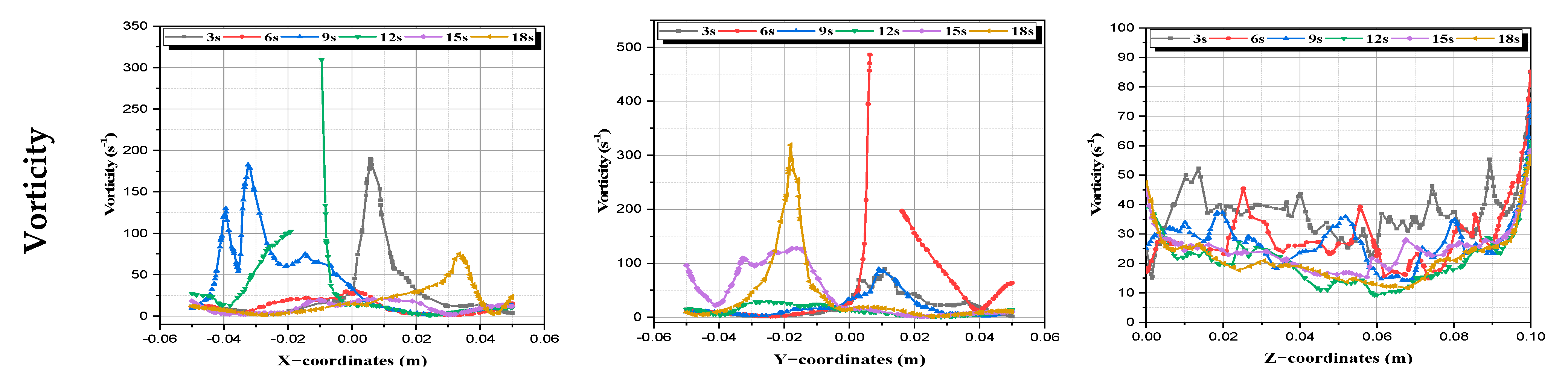
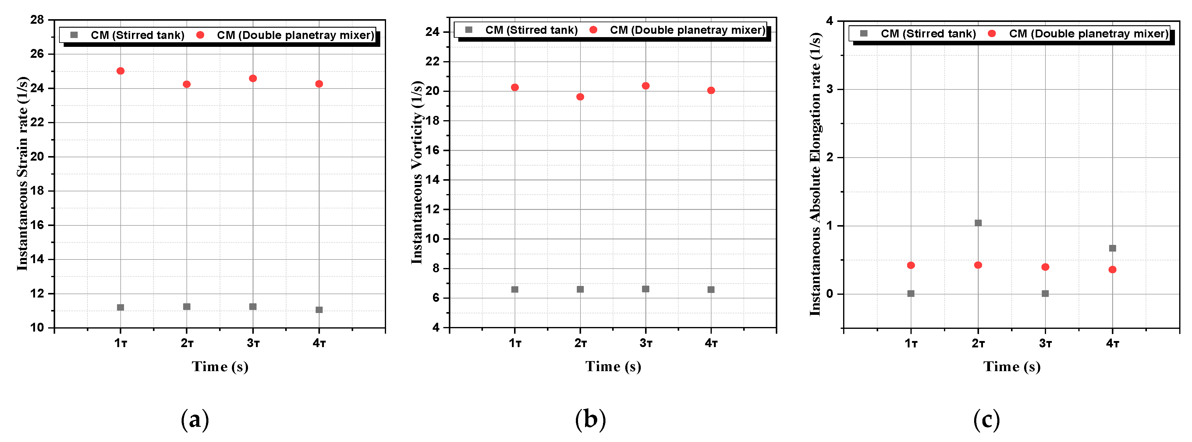
- Instantaneous kinematic properties: In order to assess the performance and the efficiency of our twisted double planetary mixer, a comparison of the instantaneous properties (strain rate, vorticity and absolute elongation) was conducted with the study already conducted by Telha et al. [3] using a stirred tank. The results shown in Figure 12 below confirm the clear superiority of the present mixer compared with the other mixer, especially with regard to the strain rate and the vorticity, which proves the efficiency of this mixer.
5. Conclusions
Author Contributions
Funding
Data Availability Statement
Conflicts of Interest
References
- Rapp, B.E.; Gruhl, F.J.; Länge, K. Biosensors with label-free detection designed for diagnostic applications. Anal. Bioanal. Chem. 2010, 398, 2403–2412. [Google Scholar] [CrossRef] [PubMed]
- El Omari, K.; Le Guer, Y. Alternaterotating walls for thermal chaotic mixing. Int. J. Heat Mass Transf. 2010, 53, 123–134. [Google Scholar] [CrossRef]
- Telha, M.; Bachiri, M.; Lasbet, Y.; Naas, T.T. Effect of Temporal modulation on the local Kinematic Process of tow-dimensional chaotic flow: A numerical analysis. J. Appl. Fluid Mech. 2021, 14, 187–199. [Google Scholar]
- Lasbet, Y.; Aidaoui, L.; Loubar, K. Effects of the Geometry Scale on the Behaviour of the Local Physical Process of the Velocity Field in the Laminar Flow. Int. J. Heat Technol. 2016, 34, 439–445. [Google Scholar] [CrossRef]
- Cartwright, J.H.E.; Eguíluz, V.M.; Hernández-García, E.; Piro, O. Dynamics of Elastic Excitable Media. Int. J. Bifurc. Chaos 1999, 11, 2197–2202. [Google Scholar] [CrossRef]
- Aref, H. The development of chaotic advection. Phys. Fluids 2002, 14, 1315–1325. [Google Scholar] [CrossRef]
- Ottino, J.M.; Ottino, J. The Kinematics of Mixing: Stretching, Chaos, and Transport; Cambridge University Press: Cambridge, UK, 1989. [Google Scholar]
- Chaiken, J.; Chevray, R.; Tabor, M.; Tan, Q.M. Experimental study of Lagrangian turbulence in a Stokes flow. Proc. R. Soc. London. Ser. A Math. Phys. Sci. 1986, 408, 165–174. [Google Scholar] [CrossRef]
- Alligood, K.T.; Sauer, T.D.; Yorke, J.A. Chaos: An Introduction to Dynamical Systems; Springer: Dordrecht, The Netherlands, 1996; ISBN 0-387-94677-2. [Google Scholar]
- Aref, H. Stirring by chaotic advection. J. Fluid Mech. 1984, 143, 1–21. [Google Scholar] [CrossRef]
- Franjione, J.G.; Ottino, J.M. Feasibility of numerical tracking of material lines and surfaces in chaotic flows. Phys. Fluids 1987, 30, 3641. [Google Scholar] [CrossRef]
- Leong, C.W.; Ottino, J.M. Experiments on mixing due to chaotic advection in a cavity. J. Fluid Mech. 1989, 209, 463–499. [Google Scholar] [CrossRef]
- Muzzio, F.J.; Swanson, P.D.; Ottino, J.M. The statistics of stretching and stirring in chaotic flows. Phys. Fluids A Fluid Dyn. 1991, 3, 822–834. [Google Scholar] [CrossRef]
- Kusch, H.A.; Ottino, J.M. Experiments on mixing in continuous chaotic flows. J. Fluid Mech. 1992, 236, 319–348. [Google Scholar] [CrossRef]
- Alvarez, M.M.; Muzzio, F.J.; Cerbelli, S.; Adrover, A. Self-Similar Spatio-Temporal Structure of Material Filaments in Chaotic Flows. Fractals Eng. 1997, 1, 323–335. [Google Scholar] [CrossRef]
- Yi, M.; Qian, S.; Haim, H. Bau A Magneto-Hydrodynamic Chaotic Stirrer. J. Fluid Mech. 2002, 468, 153–177. [Google Scholar] [CrossRef]
- Lee, C.-Y.; Fu, L.-M. Recent advances and applications of micromixers. Sens. Actuators B Chem. 2018, 259, 677–702. [Google Scholar] [CrossRef]
- Kolmogorov, A.N. On conservation of conditionally periodic motions under small perturbations of the Hamiltonian. Dokl. Akad. Nauk. SSSR 1954, 98, 527–530. [Google Scholar]
- Moser, J. On invariant curves of area-preserving mappings of an annulus. Nachr. Akad. Wiss. Gott. Math. Phys. 1962, II, 1–20. [Google Scholar]
- Arnol’D, V.I. Small denominators and problems of stability of motion in classical and celestial mechanics. Russ. Math. Surv. 1963, 18, 85–191. [Google Scholar] [CrossRef]
- Aguirre, A.; Castillo, E.; Cruchaga, M.; Codina, R.; Baiges, J. Stationary and time-dependent numerical approximation of the lid-driven cavity problem for power-law fluid flows at high Reynolds numbers using a stabilized finite element formulation of the VMS type. J. Non-Newton. Fluid Mech. 2018, 257, 22–43. [Google Scholar] [CrossRef]
- Grosso, G.; Hulsen, M.A.; Fard, A.S.; Overend, A.; Anderson, P.D. Mixing processes in the cavity transfer mixer: A thorough study. AIChE J. 2018, 64, 1034–1048. [Google Scholar] [CrossRef]
- Jung, S.Y.; Ahn, K.H.; Kang, T.G.; Park, G.T.; Kim, S.U. Chaotic mixing in a barrier-embedded partitioned pipe mixer. AIChE J. 2018, 64, 717–729. [Google Scholar] [CrossRef]
- Luan, D.; Chen, Y.; Wang, H.; Wang, Y.; Wei, X. Chaotic characteristics of pseudoplastic fluid induced by 6PBT impeller in a stirred vessel. Chin. J. Chem. Eng. 2018, 27, 293–297. [Google Scholar] [CrossRef]
- Mizuno, Y.; Funakoshi, M. Chaotic mixing due to a spatially periodic three-dimensional flow. Fluid Dyn. Res. 2002, 31, 129–149. [Google Scholar] [CrossRef]
- Mizuno, Y.; Funakoshi, M. Chaotic mixing caused by an axially periodic steady flow in a partitioned-pipe mixer. Fluid Dyn. Res. 2004, 35, 205–227. [Google Scholar] [CrossRef]
- Pacheco, J.R.; Chen, K.P.; Hayes, M.A. Rapid and efficient mixing in a slip-driven three-dimensional flow in a rectangular channel. Fluid Dyn. Res. 2006, 38, 503–521. [Google Scholar] [CrossRef]
- Xu, B.-P.; He, L.; Wang, M.-G.; Tan, S.-Z.; Yu, H.-W.; Turng, L.-S. Numerical Simulation of Chaotic Mixing in Single Screw Extruders with Different Baffle Heights. Int. Polym. Process. 2016, 31, 108–118. [Google Scholar] [CrossRef]
- Naas, T.T.; Lasbet, Y.; Aidaoui, L.; Boukhalkhal, A.; Loubar, K. Characterization of Pressure Drops and Heat Transfer of Non-Newtonian Power-Law Fluid Flow Flowing in Chaotic Geometry. Int. J. Heat Technol. 2016, 34, 251–260. [Google Scholar] [CrossRef]
- Naas, T.T.; Lasbet, Y.; Aidaoui, L.; Boukhalkhal, A.; Loubar, K. High performance in terms of thermal mixing of non-Newtonian fluids using open chaotic flow: Numerical investigations. Therm. Sci. Eng. Prog. 2020, 16, 100454. [Google Scholar] [CrossRef]
- Tayeb, N.T.; Amar, K.; Sofiane, K.; Lakhdar, L.; Yahia, L. Thermal mixing performances of shear-thinning non-Newtonian fluids inside Two-Layer Crossing Channels Micromixer using entropy generation method: Comparative study. Chem. Eng. Process. Process Intensif. 2020, 156, 108096. [Google Scholar] [CrossRef]
- Jegatheeswaran, S.; Ein-Mozaffari, F.; Wu, J. Process intensification in a chaotic SMX static mixer to achieve an energy-efficient mixing operation of non-Newtonian fluids. Chem. Eng. Process. Process Intensif. 2018, 124, 1–10. [Google Scholar] [CrossRef]
- Tohidi, A.; Hosseinalipour, S.M.; Monfared, Z.G.; Mujumdar, A.S. Laminar Heat Transfer Enhancement Utilizing Nanofluids in a Chaotic Flow. J. Heat Transf. 2014, 136, 091704. [Google Scholar] [CrossRef]
- Tohidi, A.; Hosseinalipour, S.; Shokrpour, M.; Mujumdar, A. Heat transfer enhancement utilizing chaotic advection in coiled tube heat exchangers. Appl. Therm. Eng. 2015, 76, 185–195. [Google Scholar] [CrossRef]
- Tohidi, A.; Hosseinalipour, S.; Taheri, P.; Nouri, N.; Mujumdar, A. Chaotic advection induced heat transfer enhancement in a chevron-type plate heat exchanger. Heat Mass Transf. 2013, 49, 1535–1548. [Google Scholar] [CrossRef]
- Wünsch, O.; Böhme, G. Numerical simulation of 3d viscous fluid flow and convective mixing in a static mixer. Arch. Appl. Mech. 2000, 70, 91–102. [Google Scholar] [CrossRef]
- Niederkorn, T.C.; Ottino, J.M. Chaotic mixing of shear-thinning fluids. AIChE J. 1994, 40, 1782–1793. [Google Scholar] [CrossRef]
- Leprevost, J.C.; Lefévre, A.; Brancher, J.P.; Saatdjian, E. Chaotic mixing and heat transfer in a periodic 2D flow. Comptes Rendus L’acad. Sci. Ser. II-B Mech. 1997, 9, 519–526. [Google Scholar]
- Galaktionov, O.S.; Meleshko, V.V.; Peters, G.W.M.; Meijer, H.E.H. Stokes flow in a rectangular cavity with a cylinder. Fluid Dyn. Res. 1999, 24, 81–102. [Google Scholar] [CrossRef]
- Hosseinalipour, S.M.; Tohidi, A.; Mashaei, P.R.; Mujumdar, A.S. Experimental investigation of mixing in a novel continuous chaotic mixer. Korean J. Chem. Eng. 2014, 31, 1757–1765. [Google Scholar] [CrossRef]
- Hosseinalipour, S.M.; Tohidi, A.; Shokrpour, M.; Nouri, N.M. Introduction of a chaotic dough mixer, part A: Mathematical modeling and numerical simulation. J. Mech. Sci. Technol. 2013, 27, 1329–1339. [Google Scholar] [CrossRef]
- Msaad, A.A.; Mahdaoui, M.; Kousksou, T.; Allouhi, A.; El Rhafiki, T.; Jamil, A.; Ouazzani, K. Numerical simulation of thermal chaotic mixing in multiple rods rotating mixer. Case Stud. Therm. Eng. 2017, 10, 388–398. [Google Scholar] [CrossRef]
- Shirmohammadi, F.; Tohidi, A. Mixing enhancement using chaos theory in fluid dynamics: Experimental and numerical study. Chem. Eng. Res. Des. 2019, 141, 350–360. [Google Scholar] [CrossRef]
- Aref, H.; Balachandar, S. Chaotic advection in a Stokes flow. Phys. Fluids 1986, 29, 3515. [Google Scholar] [CrossRef]
- ANSYS, Inc. ANSYS Fluent database. 2016.
- Khakhar, D.V.; Ottino, J.M. Deformation and breakup of slender drops in linear flows. J. FluidMech 1986, 166, 265–285. [Google Scholar] [CrossRef]


| Radius of Cylindrical Tank | 50 mm | Eccentricity of Rod 2 | 35 mm | ||
| Radius of cylindrical rod 1 | 5 mm | Hauteur of tank | 100 mm | ||
| Radius of cylindrical rod 2 | 5 mm | Hauteur of rods | 95 mm | ||
| Eccentricity of rod 1 | 10 mm | ||||
| Tank | Revolution Axe of Tank () |  | |
| Rod 1 | Axe 1 () | ||
| Revolution axe of the tank () | |||
| Rod 2 | Axe 1 () | ||
| Revolution axe of the tank() | |||
| (a) | (b) | ||
| Dynamic Viscosity () | Specific Heat () | ||
| Density () | Thermal conductivity () | ||
| Prandtl number () | 6780.325 | Peclet number () | 144,353 |
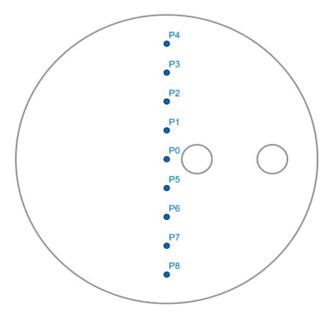
| Particle | P0 | P1 | P2 | P3 | P4 | P5 | P6 | P7 | P8 |
| X | 0 | 0 | 0 | 0 | 0 | 0 | 0 | 0 | 0 |
| Y | 0.04 | 0.03 | 0.02 | 0.01 | 0 | −0.01 | −0.02 | −0.03 | −0.04 |
| Z | 0.05 | 0.05 | 0.05 | 0.05 | 0.05 | 0.05 | 0.05 | 0.05 | 0.05 |
| P1 | P2 | |||||
|---|---|---|---|---|---|---|
| X | Y | Z | X | Y | Z | |
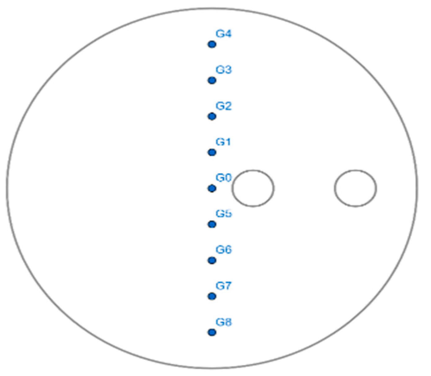
| G0 | 0 | 0 | 0.05 | 0 | 0.001 | 0.05 |
| G1 | 0 | 0.01 | 0.05 | 0 | 0.011 | 0.05 |
| G2 | 0 | 0.02 | 0.05 | 0 | 0.021 | 0.05 |
| G3 | 0 | 0.03 | 0.05 | 0 | 0.031 | 0.05 |
| G4 | 0 | 0.04 | 0.05 | 0 | 0.041 | 0.05 |
| G5 | 0 | −0.01 | 0.05 | 0 | −0.011 | 0.05 |
| G6 | 0 | −0.02 | 0.05 | 0 | −0.021 | 0.05 |
| G7 | 0 | −0.03 | 0.05 | 0 | −0.031 | 0.05 |
| G8 | 0 | −0.04 | 0.05 | 0 | −0.041 | 0.05 |
Publisher’s Note: MDPI stays neutral with regard to jurisdictional claims in published maps and institutional affiliations. |
© 2022 by the authors. Licensee MDPI, Basel, Switzerland. This article is an open access article distributed under the terms and conditions of the Creative Commons Attribution (CC BY) license (https://creativecommons.org/licenses/by/4.0/).
Share and Cite
Mostefa, T.; Eddine, A.D.; Tayeb, N.T.; Hossain, S.; Rahman, A.; Mohamed, B.; Kim, K.-Y. Kinematic Properties of a Twisted Double Planetary Chaotic Mixer: A Three-Dimensional Numerical Investigation. Micromachines 2022, 13, 1545. https://doi.org/10.3390/mi13091545
Mostefa T, Eddine AD, Tayeb NT, Hossain S, Rahman A, Mohamed B, Kim K-Y. Kinematic Properties of a Twisted Double Planetary Chaotic Mixer: A Three-Dimensional Numerical Investigation. Micromachines. 2022; 13(9):1545. https://doi.org/10.3390/mi13091545
Chicago/Turabian StyleMostefa, Telha, Aissaoui Djamel Eddine, Naas Toufik Tayeb, Shakhawat Hossain, Arifur Rahman, Bachiri Mohamed, and Kwang-Yong Kim. 2022. "Kinematic Properties of a Twisted Double Planetary Chaotic Mixer: A Three-Dimensional Numerical Investigation" Micromachines 13, no. 9: 1545. https://doi.org/10.3390/mi13091545