
Optimized Random Forest for Solar Radiation Prediction Using Sunshine Hours
 ,
,  , ,
, ,  and
and
Abstract
:1. Introduction
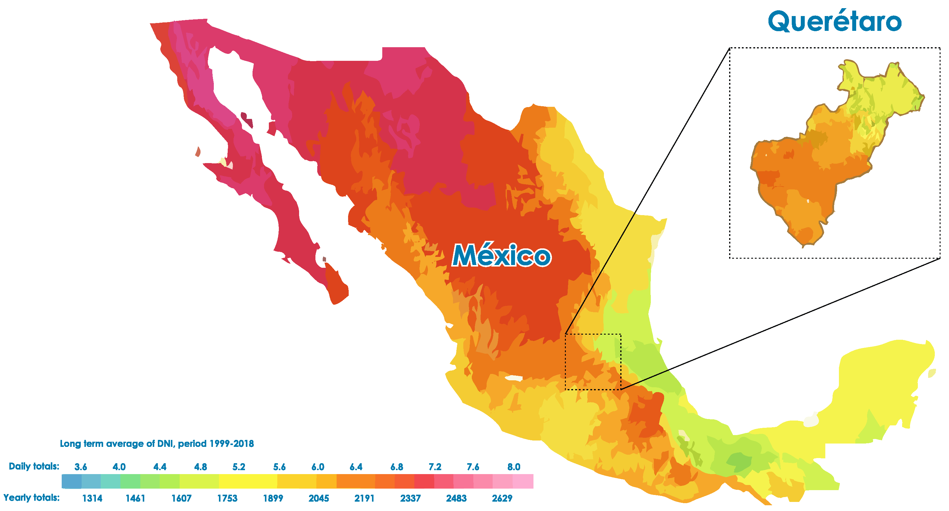
Study Area

2. Related Works
- Machine learning (RF, SVM, ANN, Kernel regression) algorithms for solar radiaton prediction
- Hybrid algorithms (combination of many algorithms) for solar radiaton prediction
- The performance metrics used by the authors identified the most used approaches, namely, R2, MAPE, MSE, and the accurac of models based on these approaches. Other performance metrics, such as the MAE or MBE, were reported as well, although only in three articles.
- Models that only predicted one type of variable (SR vs. SR and wind) have a better outcome than those that try to predict two or more variables.
- The most used ML types were identified, as were the extra algorithms used to improve their performance, with heuristic and evolutionary algorithms being the most common.
- The type of solar radiation most studied in these works was global radiation, with direct or diffuse radiation mentioned in only two articles.
- In order to determine which types of hyperparameters were used in each model, the most representative alternatives for optimizing the RF algorithm were considered. In Section 3.5, we provide a list of the hyperparameters we used and how each affected performance in this study.

| Year | Reference | Classification | Algorithm | Kernel (only for SVM) | R | Mean Absolute Error (MAE) | Root Mean Square Error (RMSE) |
|---|---|---|---|---|---|---|---|
| 2017 | Quej et al. [26] | Machine Learning | SVM/ANFIS/ ANN | RBF | 0.689 | 1.973 | 2.678 |
| 2018 | Gupta et al. [27] | Hybrid | RF + Genetic | – | 24.45 | – | 47.74 |
| 2019 | Ghazvinian et al. [28] | Hybrid | SVM + PSO | RBF | 9.01–0.141 | – | 19.10 |
| 2019 | Srivastava et al. [29] | Machine Learning | Random Forest | – | – | 15.74 | 65.08 |
| 2020 | Sun et al. [30] | Tree Based | Adaboost | – | – | 8.41 | – |
| 2020 | Pang et al. [20] | Neural Network | RNN/MLP | – | 0.983 | – | 41.2 |
| 2021 | Zhu et al. [21] | Neural Network | CNN, LSTM | 30 | 0.958 | 23.89 | |
| 2021 | Aljanad et al. [31] | Hybrid | BPNN-PSO | – | 0.7537 | – | 1.7078 |
| 2021 | Philibus et al.[32] | Hybrid | ANN/SVM | RBF | 0.9112 | 0.1842 | 0.1014 |
| 2022 | Faisal et al. [33] | Neural Network | RNN, LSTM, GRU | – | 128 | 0.918 | 0.958 |
| 2022 | Brahma et al. [34] | Deep Learning | Multi-Step CNN Stacked LSTM | – | 68.62 | 9.721 | 9.859 |
3. Theoretical Bases
3.1. The 80–20 Rule
3.2. Pearson Correlation
3.3. Distance Correlation
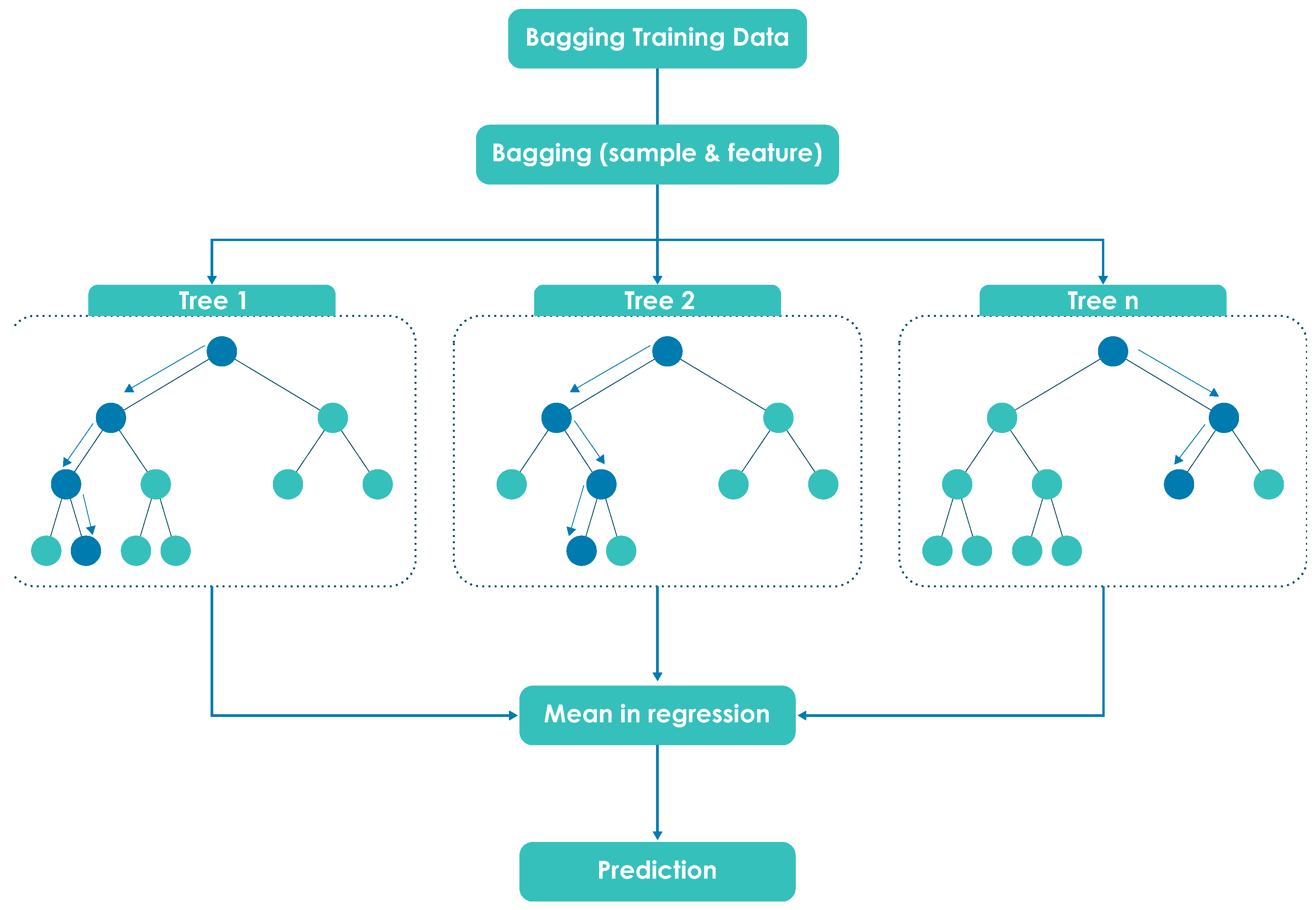
3.4. Random Forest for Regression
3.5. Hyperparameter Optimization
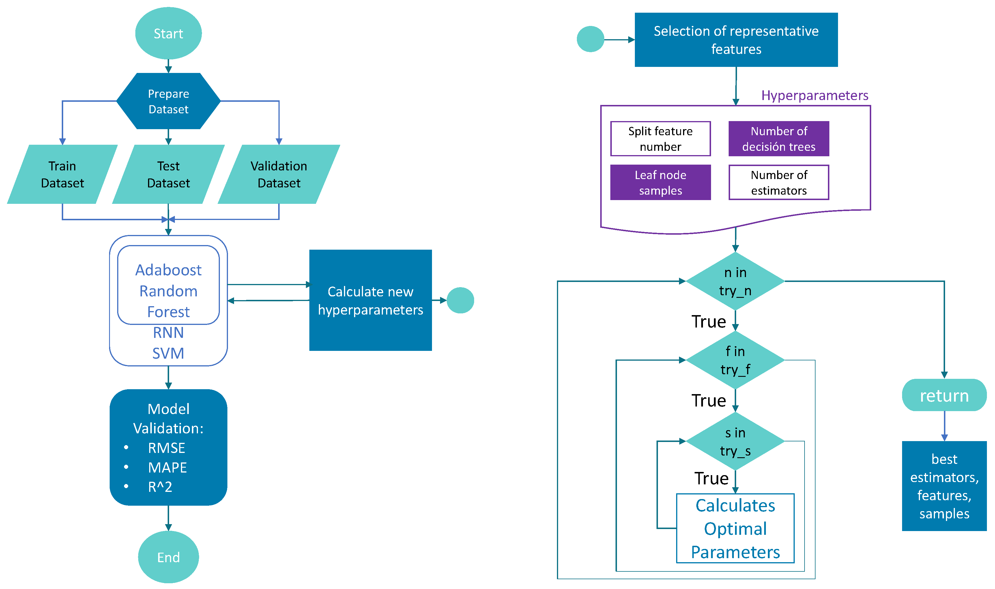
3.6. Finding the Best Combination of Tunable Hyperparameters for the Random Forest Regressor
- n_estimators In general, more estimators is better, although it has the disadvantage of decreasing yield. As is evident, more trees leads to a longer computation time. One of the great challenges of this algorithm is to find the critical number of decision trees where the best accuracy is obtained while balancing the computation time.
- max_features This is the maximum number before cutting to a new node. If certain trees consider a different subset of features than others, the correlation between those two groups should be minimal. This is desirable because it allows the influence of each feature to be assessed individually.
- maximum_depth Having trees with too much depth effectively leads to overfitting. There is a critical depth at which trees are split deep enough to obtain a useful fit without being overly influenced by individual values. A depth constraint can be created by adjusting the parameters (min_samples_split), (min_samples_leaf), (min_weight_fraction_leaf), or (max_leaf_nodes), rather than specifying a preset value for the depth.
| Algorithm 1 Stages of the proposed Random Forest Optimizer. |
Input: estimators, features, samples. Output: model, bestE, bestF, bestS.
|
3.7. Statistical Metrics for Data Validation
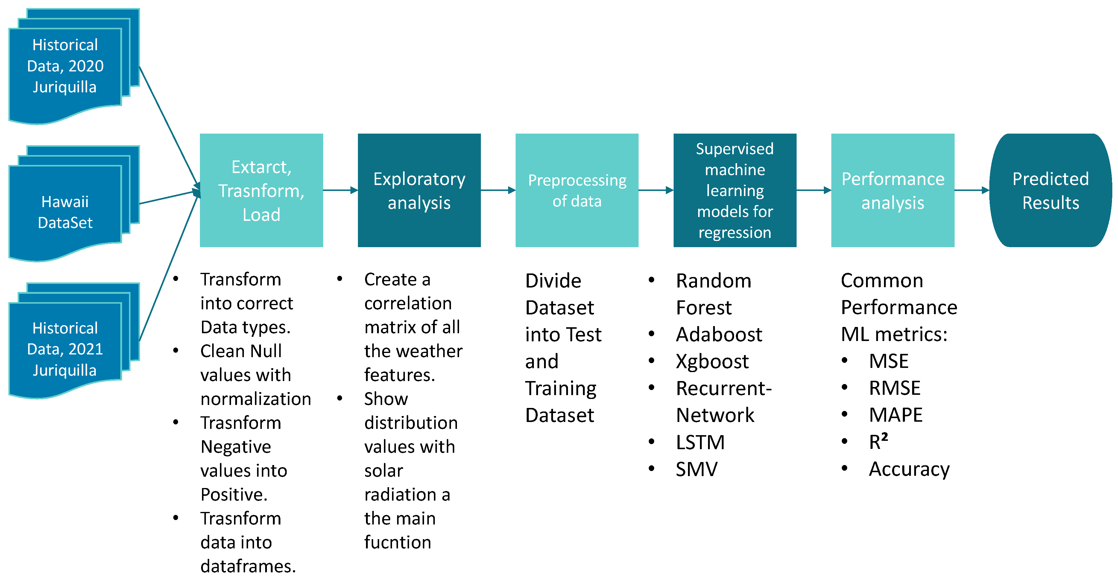
4. Materials and Methods
Dataset
- SR:
- Temperature:
- Humidity: measured in percent
- Barometric pressure:
- Wind direction: measured in degrees
- Wind speed:
- Sunrise/sunset: Queretaro Time (GMT-5)
5. Results
- Remove corrupt or unreadable data;
- Replace all non-numerical data in all columns with numerical and floating values;
- Replace all missing or zero values through normalization techniques;
- Apply label coding to all columns.
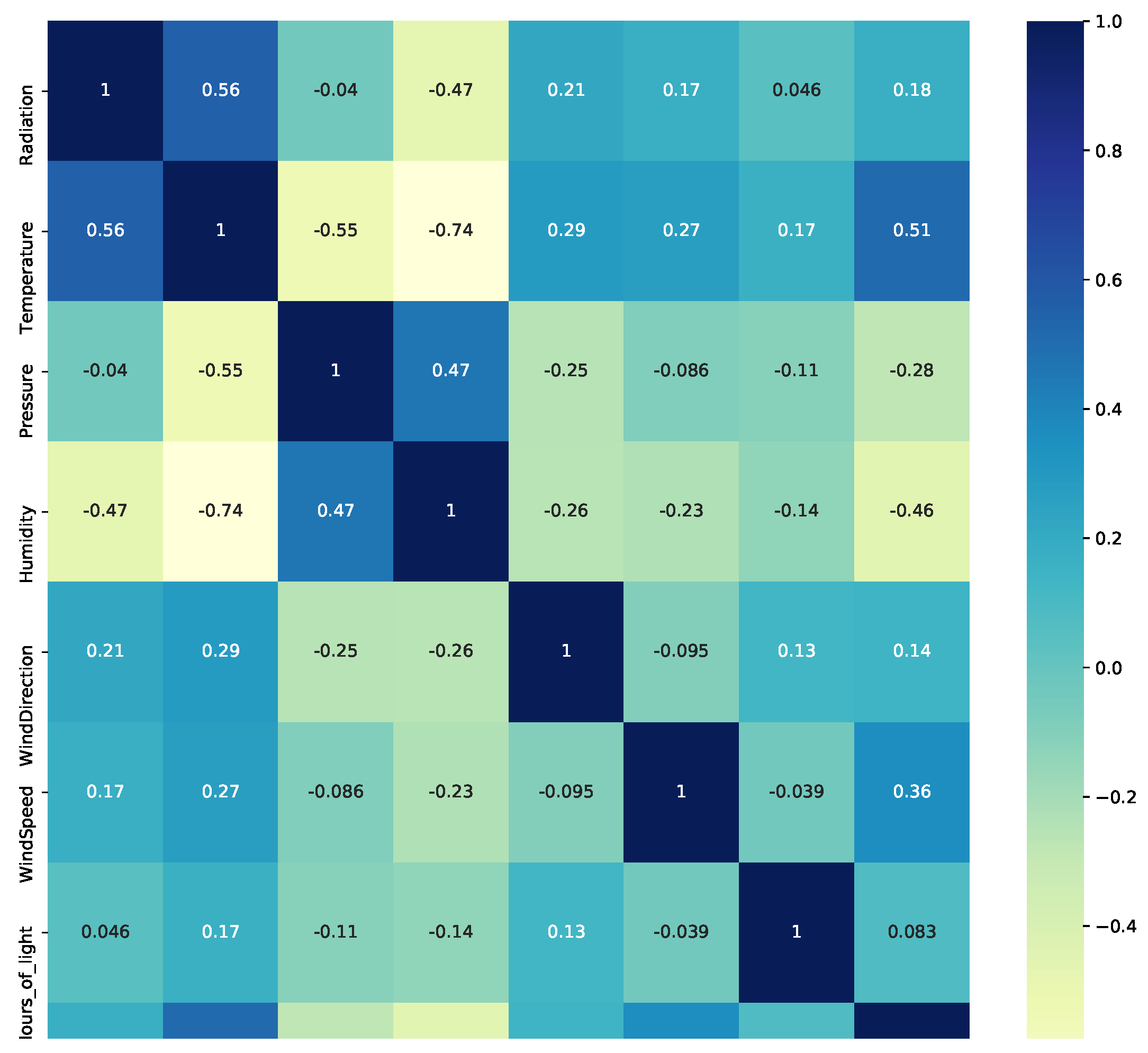
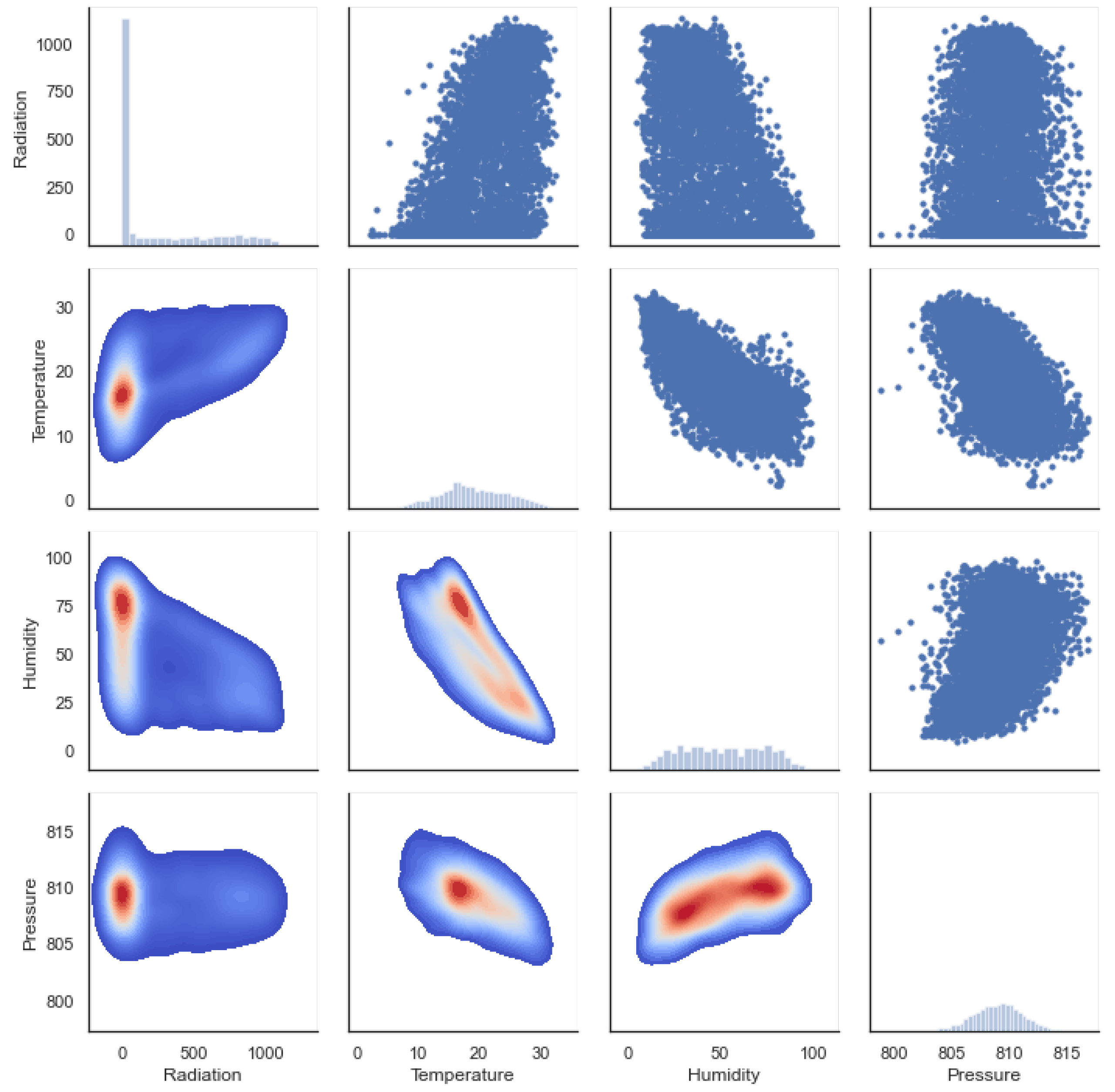
5.1. Heat Map and Pearson Correlation
5.2. Distance Correlation
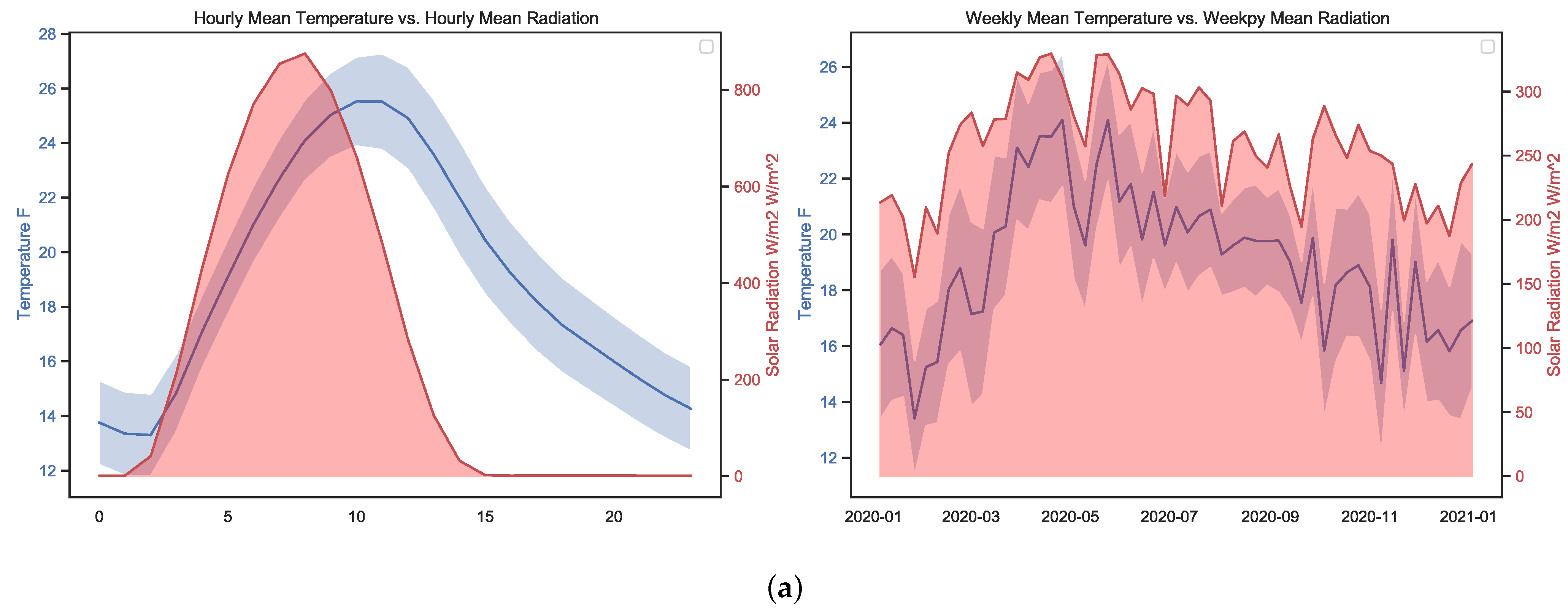
- The higher the detected temperature, the higher the amount of SR; this can be seen from the Pearson correlation value R of 0.56 and the relationship observable in Figure 7a between radiation and temperature on hourly and weekly scales. The distance correlation of 0.55 means that there is a relationship between temperature and SR.
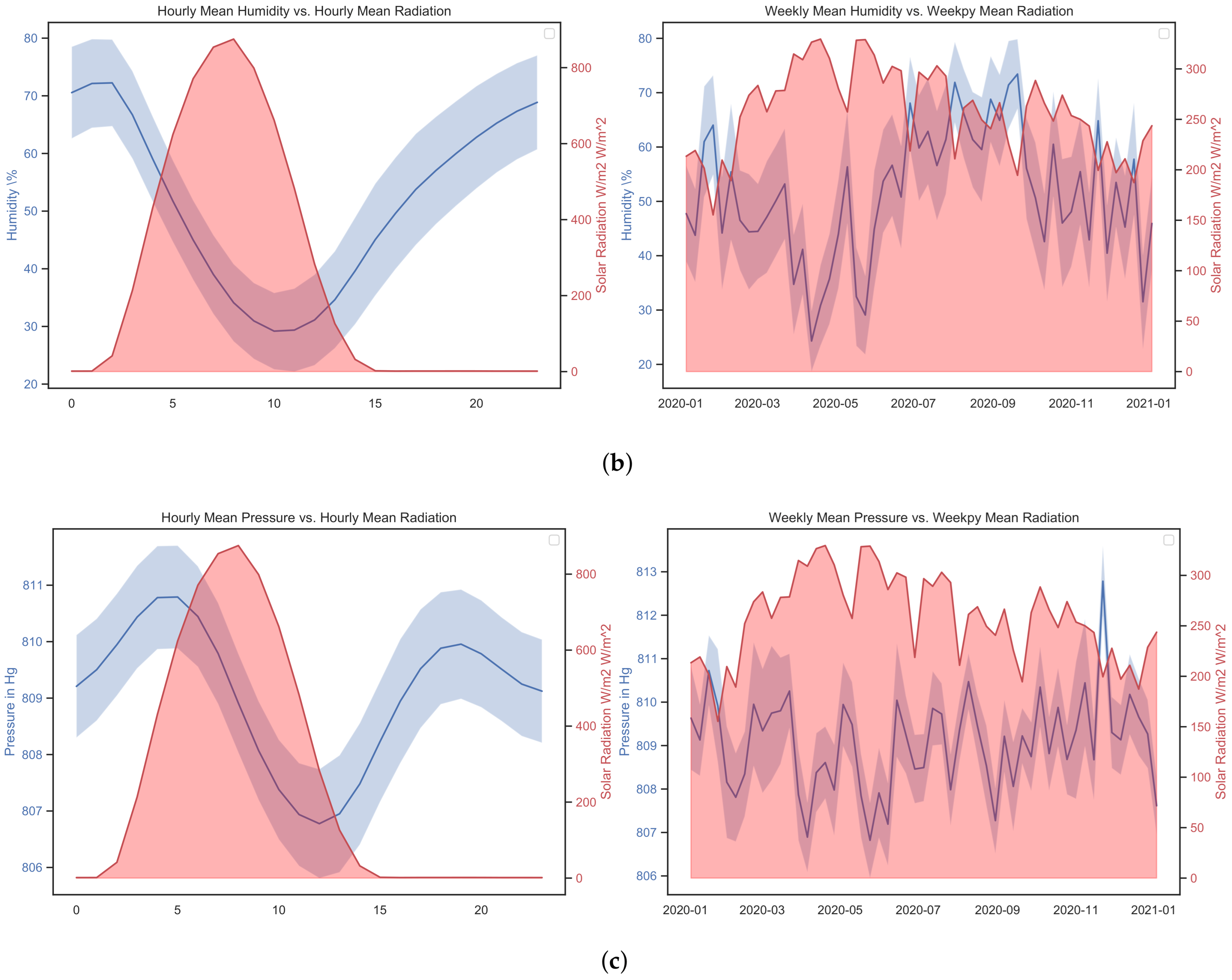
- Humidity has an inverse or negative relationship with RH compared to temperature, and is potentially significant and cannot be ignored as a potential driver in the climate system. This can be observed in Figure 7 on both the hourly time scale and to a lesser extent on the weekly scale.
- Based on both the Pearson and distance correlations, pressure does not seem to have a direct relationship with SR, although it is related to temperature and humidity. Related work can be found in [44].
- The variables of wind speed and direction variables are not relevant for this study; while a correlation can be observed, this does not mean imply any causality.
- While Queretaro is a city without significant seasonal changes, during the rainy and summer period significant changes can be observed, as can be seen in the weekly graphs in Figure 7.
- The weekly time scale is the best for forecasting. The month-to-month variations are substantial and do not capture the seasonal changes over the course of the year. Minute time scales are helpful for more refined work such as PV control systems. Hourly time scales are good, although they can be noisy if not filtered properly.
5.3. Machine Learning for Solar Radiation Prediction
- Recurrent NN regression
- SVM regression
- Random Forest regression
- Adaboost regression
- Optimized RF regression
- Optimized Adaboost regression
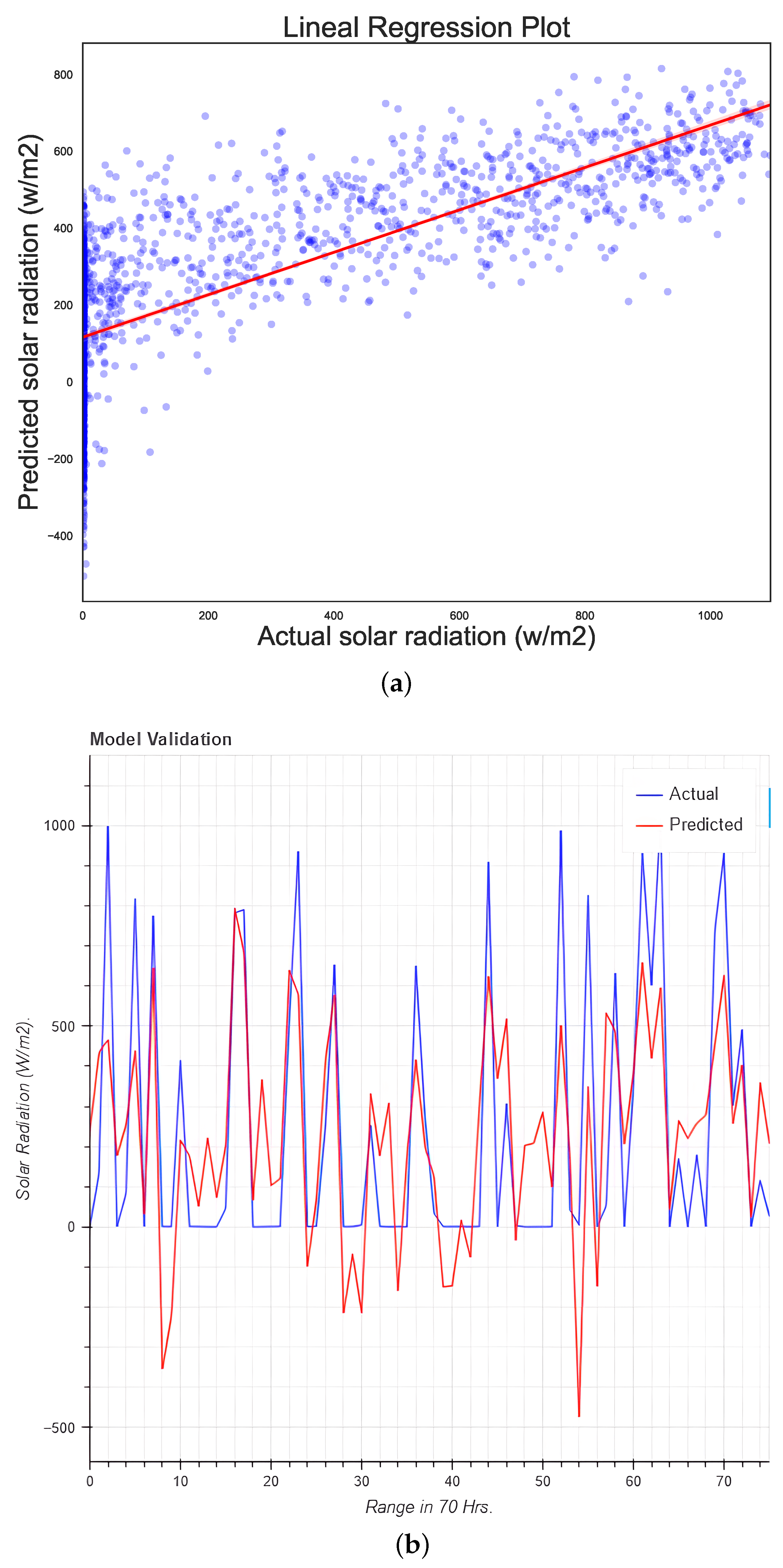
5.4. Simple Linear Regression
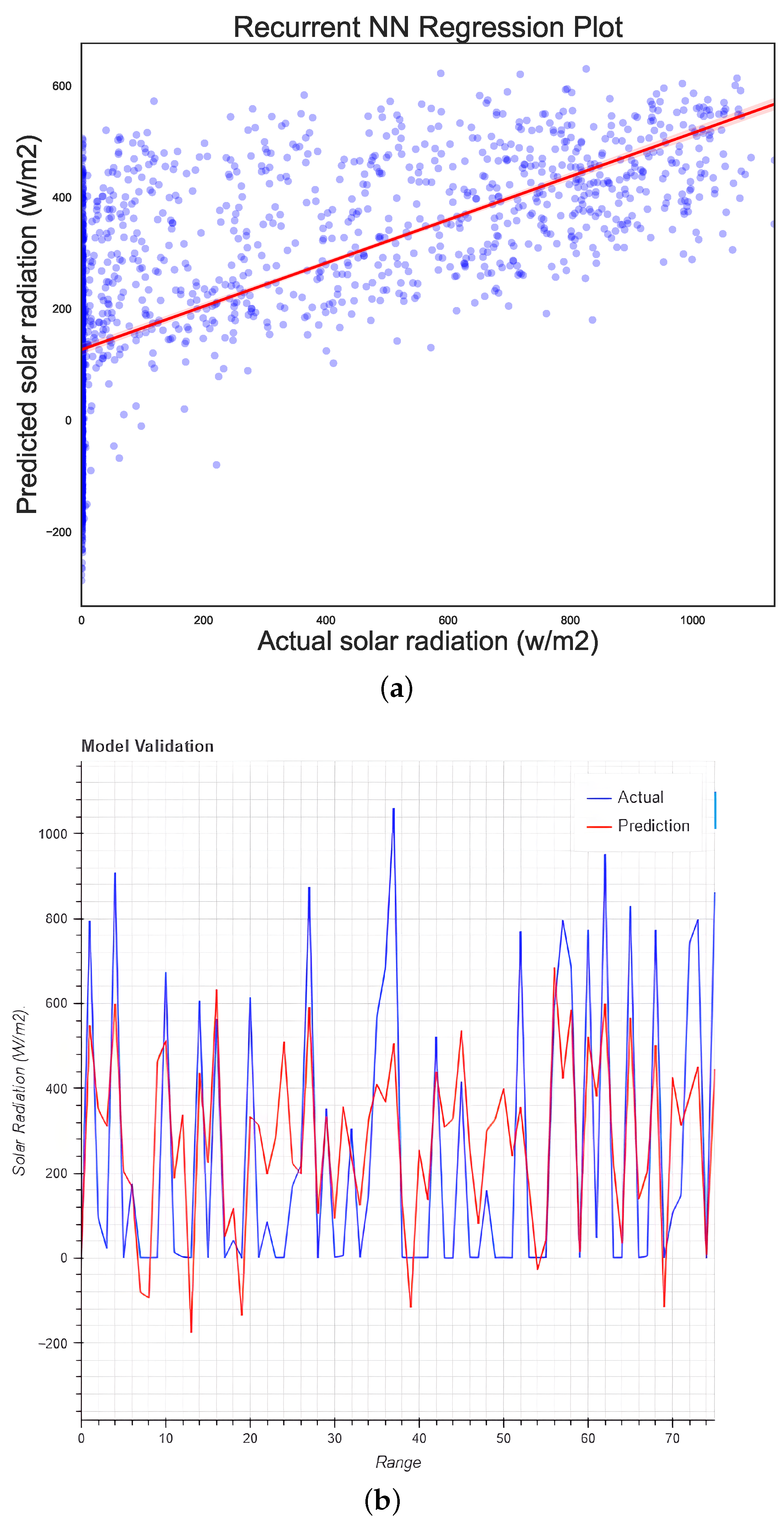
5.5. Recurrent Neural Network Regression
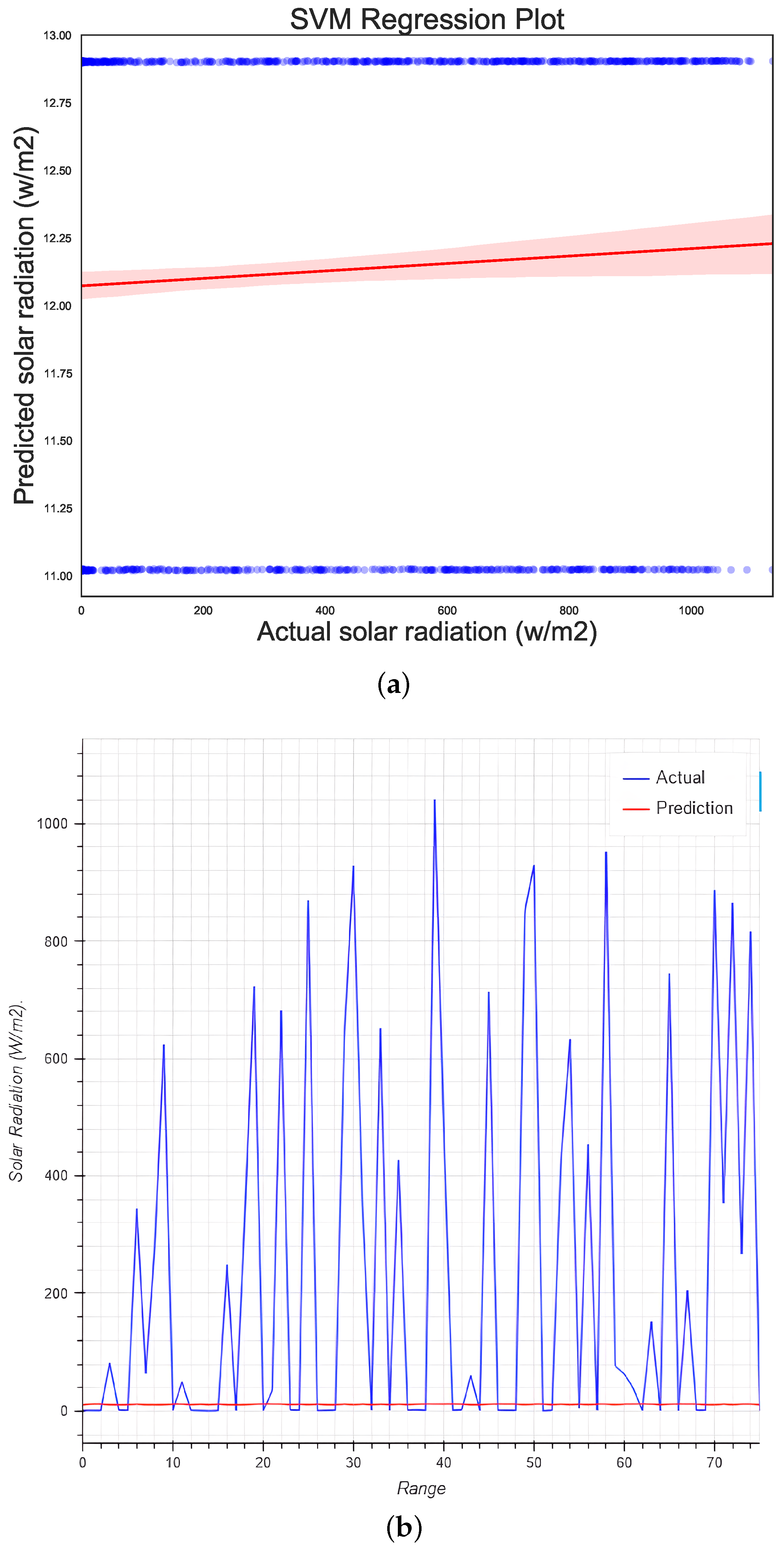
5.6. Support Vector Regression
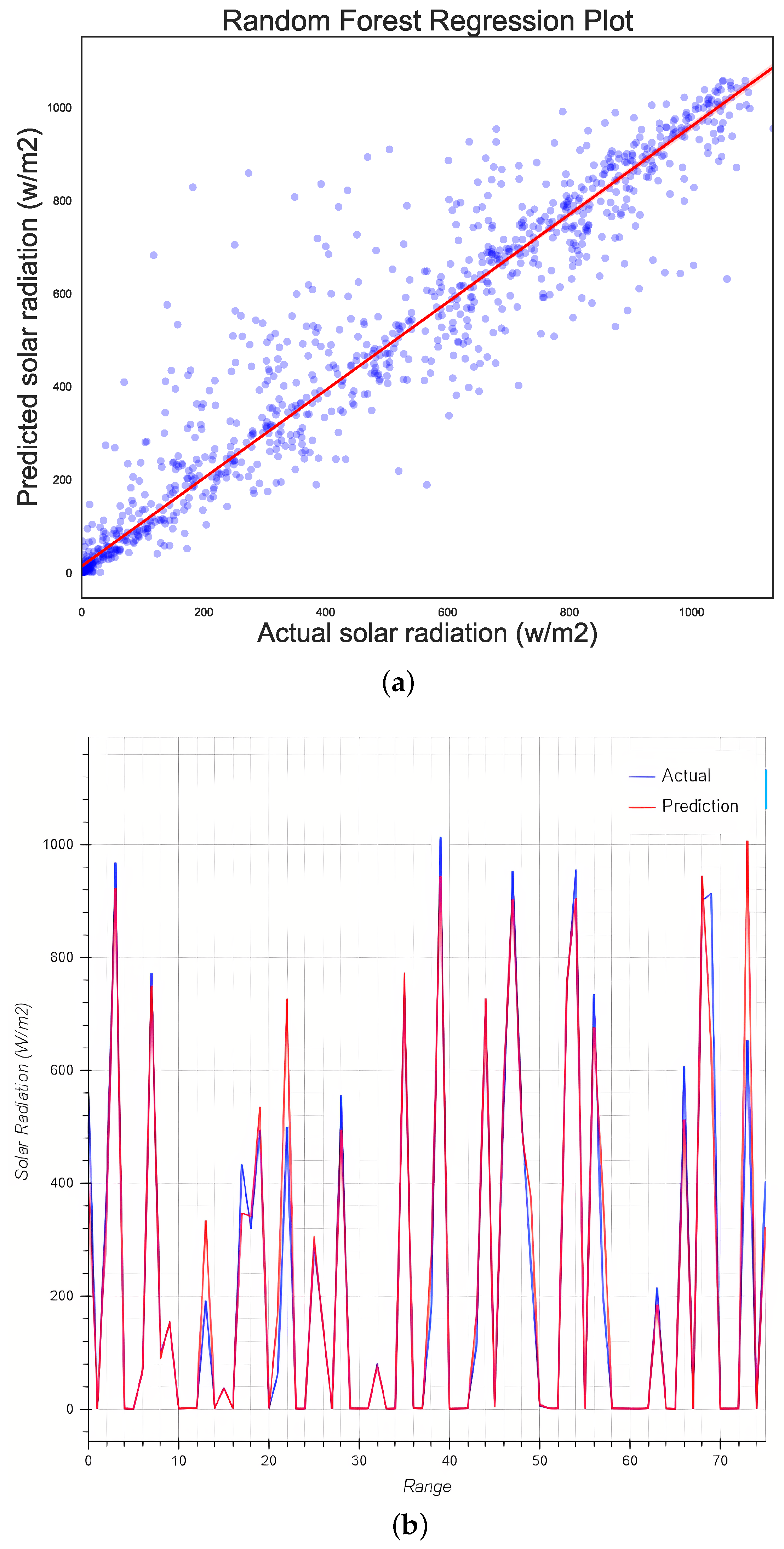
5.7. Random Forest Regression
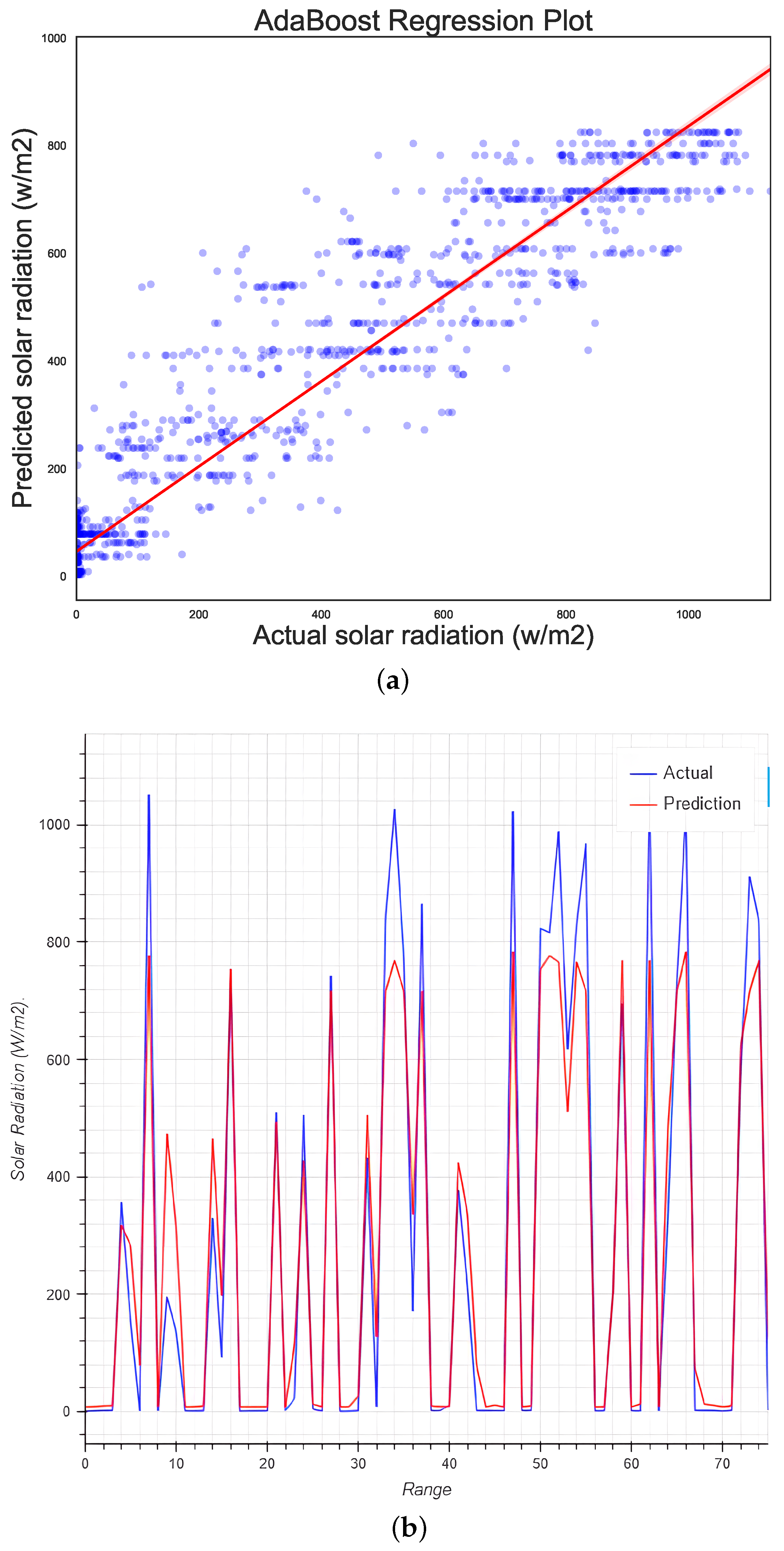
5.8. Adaboost Regression
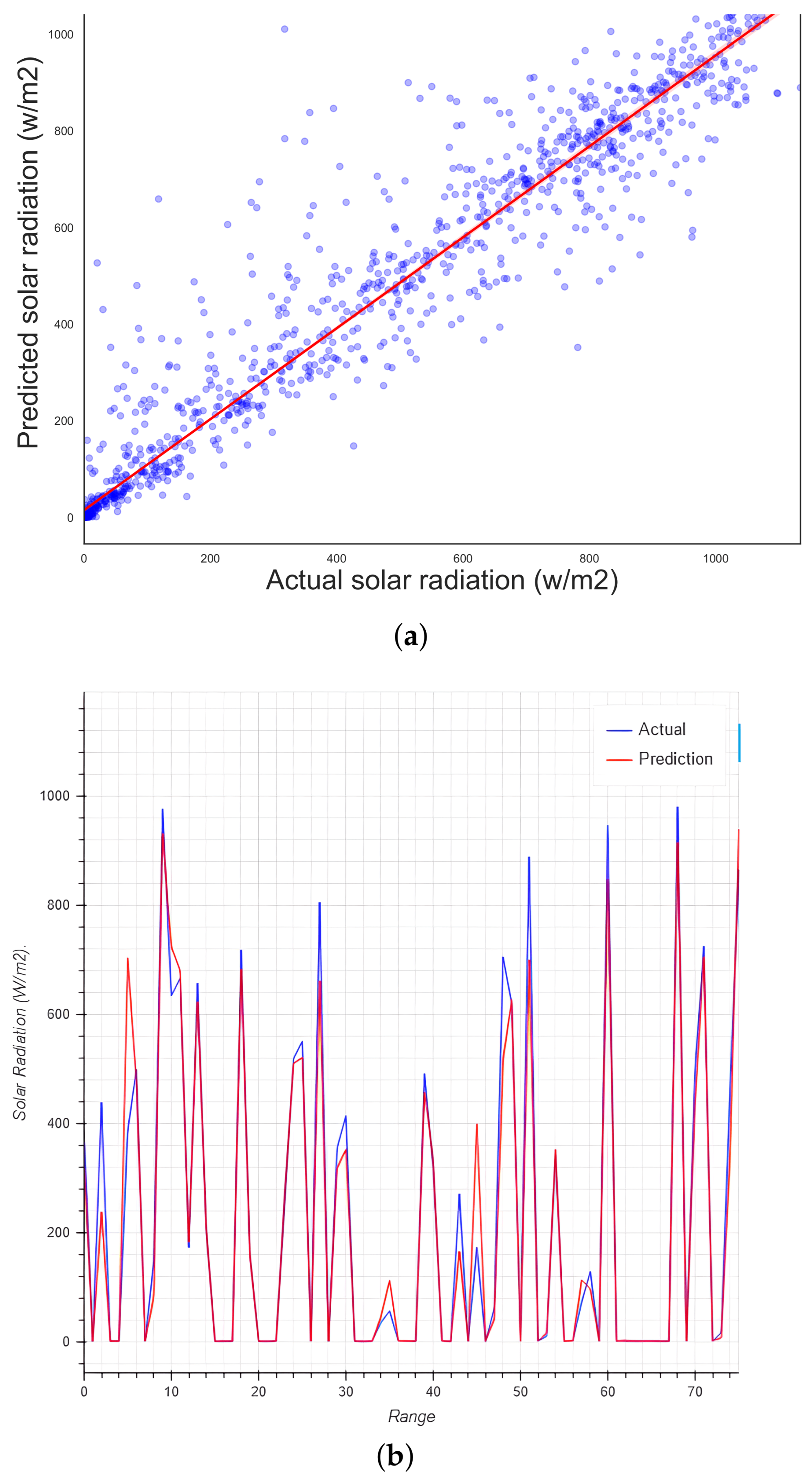
5.9. Optimized Hyperparameters Random Forest
5.10. Numerical Results
6. Discussion
- Regarding the distribution of data, for example, SVM-based algorithms tend to have improved performance on small datasets; on the contrary, as can be seen in our results, tree-based algorithms (RF, Adaboost, XGboost) tend to achieve excellent results on larger datasets.
- In the preliminary inspection of the data, we found several instances in which no data was collected, especially in December and early January, presumably due to a lack of personnel to maintain the site. Much time was consumed ensuring that the dataset was complete and that the information was accurate and reliable, beyond the preparation described in this article.
- Another reason is that the parameter selection of the machine learning models could not find the optimal global solution.
- Performing a statistical analysis of the data is essential, especially for time series, including finding the mean, maxima, and minima of the data, checking its variance, and determining whether the type of regression or prediction method is appropriate.
- Several articles have pointed out that different meteorological factors such as air temperature, relative humidity, wind speed, and precipitation are closely related to solar radiation, although the effects and the degrees to which they affect it can vary according to the different regions or countries under investigation.
- Differences in the implementation of algorithms can directly affect both performance and the obtained results. There are many ML libraries available for research such as that described in this article, including libraries such as Pytorch, scikit-learn, and SciPy, among others.
7. Conclusions
- There is a relationship between the variables of SR and temperature, as proven by simple linear regression; this relationship is dependent on the humidity in the city.
- The simple linear regression model has a good fit at the time of prediction.
- The random forest regression model has the best fit, as at the beginning of SR prediction the proposed optimization only managed to obtain a 3–4% increase (depending on the used dataset).
- Our results can serve as a basis for future experiments, work with other types of neural networks such as recurring ones, application of kernel regression, etc.
- The data obtained in this study can be used in solar control systems, such as PV MPPT systems, to optimize their efficiency.
- Our results can optimize the placement of renewable energy plants throughout the state of Queretaro.
Future Work
- Tree-based models allow for extracting the importance of different characteristics in determining the regression model. By looking at the importance of the different features, it is possible to understand whether the two models assign the same importance to different parameters.
- The RF algorithm performed very well from the beginning, without any need to optimize hyperparameters or specific data; yet, this selection was purely arbitrary, without any way to check whether they were the most suitable for the task.
- Iterating through a list of arbitrary values and choosing the one that provides the best results is not the best approach to optimization. It would be beneficial to spend more time tuning, perhaps including an analytical method for determining optimal values.
- Other features, such as ozone and contaminant gases, could be considered, as these features are known to impact light transmission through the atmosphere, especially at certain wavelengths.
- It is characterized by a high variance in prediction
- It appears to systematically overestimate SR after sunset
Author Contributions
Funding
Institutional Review Board Statement
Informed Consent Statement
Data Availability Statement
Acknowledgments
Conflicts of Interest
Abbreviations
| AI | Artificial Intelligence |
| ANN | Artificial Neural Networks |
| A&P | Angstrom and Prescott |
| BCM | Bergen Climate Model |
| CNN | Convolutional Neural Network |
| LR | Linear Regression |
| ML | Machine Learning |
| MLP | Multi-Layered Perceptron |
| MLP | Multi-Layered Perceptron Regression |
| PSO | Particle Swarm Optimization |
| RE | Renewable Energy |
| RF | Random Forest |
| SL | Supervised Learning |
| SVM | Support Vector Machine |
| SVMR | Support Vector Machine Regression |
| UL | Unsupervised Learning |
| RMSE | Root Mean Square Error |
| MAPE | Mean Absolute Percentage Error |
| MAE | Mean Absolute Error |
| MSE | Mean Square Error |
| PV | Photvoltaic |
References
- Islam, M.; Al-Alili, A.; Kubo, I.; Ohadi, M. Measurement of solar-energy (direct beam radiation) in Abu Dhabi, UAE. Renew. Energy 2009, 35, 515–519. [Google Scholar] [CrossRef]
- Beer, C.; Reichstein, M.; Tomelleri, E.; Ciais, P.; Jung, M.; Carvalhais, N.; Rödenbeck, C.; Arain, M.A.; Baldocchi, D.; Bonan, G.B.; et al. Terrestrial Gross Carbon Dioxide Uptake: Global Distribution and Covariation with Climate. Science 2010, 329, 834–838. [Google Scholar] [CrossRef] [PubMed]
- Cai, W.; Collins, M. Changing El Niño–Southern Oscillation in a warming climate. Nat. Rev. Earth Environ. 2021, 2, 628–644. [Google Scholar] [CrossRef]
- Wengel, C.; Lee, S.S.; Stuecker, M.; Axel Timmermann, J.E.C.; Schloesser, F. Future high-resolution El Niño/Southern Oscillation dynamics. Inst. Basic Sci. 2021, 11, 758–765. [Google Scholar] [CrossRef]
- Ohunakin, O.S.; Adaramola, M.S.; Oyewola, O.M.; Matthew, O.J.; Fagbenle, R.O. The effect of climate change on solar radiation in Nigeria. Sol. Energy 2015, 116, 272–286. [Google Scholar] [CrossRef]
- Liu, Y.; Tan, Q.; Pan, T. Determining the Parameters of the Ångström-Prescott Model for Estimating Solar Radiation in Different Regions of China: Calibration or Modeling. Earth Space Sci. 2019, 6, 1976–1986. [Google Scholar] [CrossRef]
- Vardavas, I.; Vardavas, I.; Taylor, F. Radiation and Climate: Atmospheric Energy Budget from Satellite Remote Sensing; Oxford University Press: Oxford, UK, 2011; Volume 138. [Google Scholar]
- Contreras-Sepulveda, W. Angstrom and Prescott empirical model to estimate solar radiation in North of Santander, Colombia. Rev. Investig. Desarollo Inovacion 2021, 11, 413–427. [Google Scholar] [CrossRef]
- Orozco, E.A.B.; Montes, M.V.C. Aplicación del modelo de armstrong-prescott para la estimación de la radiación solar media a nivel superficie en la ciudad de guatemala de 1995 A 2019. Rev. La Esc. Estud. Postgrado 2020, 1, 33–40. [Google Scholar]
- Leonaldo, J.; De Souza, J.; Lyra, G.; Manoel, C.; Santos, C.; Ferreira junior, R.; Tiba, C.; Lyra, G.; Antonio, M.; Lemes, M. Empirical models of daily and monthly global solar irradiation using sunshine duration for Alagoas State, Northeastern Brazil. Sustain. Energy Technol. Assess. 2016, 14, 35–45. [Google Scholar] [CrossRef]
- Almorox, J.; Bocco, M.; Willington, E. Estimation of daily global solar radiation from measured temperatures at Cañada de Luque, Córdoba, Argentina. Renew. Energy 2013, 60, 382–387. [Google Scholar] [CrossRef]
- Gielen, D.; Saygin, D.; Wagner, N.; Gutiérrez, L.I.; Torres, E.R.N. Renewable Energy Sources: Mexico. REmap 2030 Analysis 2015. Available online: https://www.irena.org/-/media/Files/IRENA/Agency/Publication/2015/IRENA_REmap_Mexico_report_2015.pdf (accessed on 10 July 2022).
- Estrada, J.E.; Santoyo, J.H.; Montesinos, J.A.O. Prospectiva del Sector Eléctrico 2013–2027. 2013. Available online: https://www.gob.mx/cms/uploads/attachment/file/62949/Prospectiva_del_Sector_El_ctrico_2013-2027.pdf (accessed on 12 June 2022). (Energy Secretary of Mexico).
- de Jesús Nieto Pérez, M.; Piñón, J.P.; Elling, R.P.; López, G.A.R.; Hurtado, M.A.V. Energías Alternativas en CICATA, Querétaro. 2010. (Consejo de Ciencia y Tecnología del Estado de Querétaro (CONCYTEQ)). Available online: http://www.concyteq.edu.mx/nthe1/pdfs/Energiasalternativasencicata.pdf (accessed on 15 July 2022).
- Sanchez, V. Sonora Podria Abastecer de Energía a Todo México con Tecnología Fotovoltaica. Available online: http://www.cienciamx.com/index.php/tecnologia/energia/329-reportaje-con-la-radiacion-solar-que-recibe-el-1-de-sonora-se-podria-generar-energia-suficiente-para-todo-el-pais (accessed on 15 April 2022).
- Suri, M.; Betak, J.; Rosina, K. Global Photovoltaic Power Potential by Country; World Bank Group: Washington, DC, USA, 2020. [Google Scholar]
- Macías, G. Radiación Solar Convertiría en Potencia a Querétaro. Diario de Queretaro. Available online: https://www.diariodequeretaro.com.mx/local/radiacion-solar-convertiria-en-potencia-a-queretaro-8219266.html (accessed on 1 May 2022).
- Alvarado, J.A.; Rios-Moreno, G.; Herrera-Ruiz, G.; Ventura-Ramos, E.; Trejo-Perea, M. Statistical analysis for the evaluation of solar and wind resources, measured in Querétaro. In Proceedings of the 2018 XIV International Engineering Congress (CONIIN), Queretaro, Mexico, 14–19 May 2018; pp. 1–8. [Google Scholar] [CrossRef]
- Hernandez Escobedo, Q.; Ramirez Jimenez, A.; Dorador-Gonzalez, J.M.; Perea-Moreno, M.A.; Perea, A. Sustainable Solar Energy in Mexican Universities. Case Study: The National School of Higher Studies Juriquilla (UNAM). Sustainability 2020, 12, 3123. [Google Scholar] [CrossRef]
- Pang, Z.; Niu, F.; O’Neill, Z. Solar radiation prediction using recurrent neural network and artificial neural network: A case study with comparisons. Renew. Energy 2020, 156, 279–289. [Google Scholar] [CrossRef]
- Zhu, T.; Guo, Y.; Li, Z.; Wang, C. Solar Radiation Prediction Based on Convolution Neural Network and Long Short-Term Memory. Energies 2021, 14, 8498. [Google Scholar] [CrossRef]
- Shamshirband, S.; Mohammadi, K.; Chen, H.; Narayana Samy, G.; Petković, D.; Ma, C. Daily global solar radiation prediction from air temperatures using Kernel Extreme Learning Machine: A case study for Iran. J. Atmos. Sol.-Terr. Phys. 2015, 134, 109–117. [Google Scholar] [CrossRef]
- Meng, M.; Song, C. Daily Photovoltaic Power Generation Forecasting Model Based on Random Forest Algorithm for North China in Winter. Sustainability 2020, 12, 2247. [Google Scholar] [CrossRef]
- Lee, J.; Wang, W.; Harrou, F.; Sun, Y. Reliable solar irradiance prediction using ensemble learning-based models: A comparative study. Energy Convers. Manag. 2020, 208, 112582. [Google Scholar] [CrossRef]
- Eseye, A.T.; Zhang, J.; Zheng, D. Short-term photovoltaic solar power forecasting using a hybrid Wavelet-PSO-SVM model based on SCADA and Meteorological information. Renew. Energy 2018, 118, 357–367. [Google Scholar] [CrossRef]
- Quej, V.H.; Almorox, J.; Arnaldo, J.A.; Saito, L. ANFIS, SVM and ANN soft-computing techniques to estimate daily global solar radiation in a warm sub-humid environment. J. Atmos. Sol.-Terr. Phys. 2017, 155, 62–70. [Google Scholar] [CrossRef]
- Gupta, S.; Katta, A.R.; Baldaniya, Y.; Kumar, R. Hybrid Random Forest and Particle Swarm Optimization Algorithm for Solar Radiation Prediction. In Proceedings of the 2020 IEEE 5th International Conference on Computing Communication and Automation (ICCCA), Greater Noida, India, 30–31 October 2020; pp. 302–307. [Google Scholar] [CrossRef]
- Ghazvinian, H.; Mousavi, S.F.; Karami, H. Integrated support vector regression and an improved particle swarm optimization-based model for solar radiation prediction. PLoS ONE 2019, 14, e0217634. [Google Scholar]
- Srivastava, R.; Tiwari, A.; Giri, V. Solar radiation forecasting using MARS, CART, M5, and random forest model: A case study for India. Heliyon 2019, 5, e02692. [Google Scholar] [CrossRef] [Green Version]
- Sun, W.; Zhang, T.; Tao, R.; Wang, A. Short-Term Photovoltaic Power Prediction Modeling Based on AdaBoost Algorithm and Elman. In Proceedings of the 2020 10th International Conference on Power and Energy Systems (ICPES), Chengdu, China, 25–27 December 2020; pp. 184–188. [Google Scholar] [CrossRef]
- Aljanad, A.; Tan, N.M.L.; Agelidis, V.G.; Shareef, H. Neural Network Approach for Global Solar Irradiance Prediction at Extremely Short-Time-Intervals Using Particle Swarm Optimization Algorithm. Energies 2021, 14, 1213. [Google Scholar] [CrossRef]
- Philibus, E.; Sallehuddin, R.; Yussof, Y.; Yusuf, L.M. Global Solar Radiation Forecasting using Artificial Neural Network and Support Vector Machine. J. Physics Conf. Ser. 2021, 2129, 012079. [Google Scholar] [CrossRef]
- Faisal, A.F.; Rahman, A.; Habib, M.T.M.; Siddique, A.H.; Hasan, M.; Khan, M.M. Neural networks based multivariate time series forecasting of solar radiation using meteorological data of different cities of Bangladesh. Results Eng. 2022, 13, 100365. [Google Scholar] [CrossRef]
- Brahma, B.; Wadhvani, R. Solar Irradiance Forecasting Based on Deep Learning Methodologies and Multi-Site Data. Symmetry 2020, 12, 1830. [Google Scholar] [CrossRef]
- Serey, J.; Quezada, L.; Alfaro, M.; Fuertes, G.; Vargas, M.; Ternero, R.; Sabattin, J.; Duran, C.; Gutierrez, S. Artificial Intelligence Methodologies for Data Management. Symmetry 2021, 13, 2040. [Google Scholar] [CrossRef]
- Edelmann, D.; Mori, T.F.; Szekely, G.J. On relationships between the Pearson and the distance correlation coefficients. Stat. Probab. Lett. 2021, 169, 108960. [Google Scholar] [CrossRef]
- Jebli, I.; Belouadha, F.Z.; Kabbaj, M.I.; Tilioua, A. Prediction of solar energy guided by pearson correlation using machine learning. Energy 2021, 224, 120109. [Google Scholar] [CrossRef]
- Szekely, G.; Rizzo, M.; Bakirov, N. Measuring and Testing Dependence by Correlation of Distances. Ann. Stat. 2008, 35, 2769–2794. [Google Scholar] [CrossRef]
- Breiman, L. Random Forests. Mach. Learn. 2001, 45, 5–32. [Google Scholar] [CrossRef] [Green Version]
- Natarajan, V.A.; Kumari, N.S. Wind Power Forecasting Using Parallel Random Forest Algorithm. In Soft Computing for Problem Solving; Springer: Singapore, 2020; pp. 209–224. [Google Scholar]
- Wu, H.; Ying, W. Benchmarking Machine Learning Algorithms for Instantaneous Net Surface Shortwave Radiation Retrieval Using Remote Sensing Data. Remote Sens. 2019, 11, 2520. [Google Scholar] [CrossRef]
- Alvarez-Alvarado, J.M.; Moreno, J.G.R.; Ventura-Ramos, E.J.; Ronquillo-Lomeli, G.; Trejo-Perea, M. An alternative methodology to evaluate sites using climatology criteria for hosting wind, solar, and hybrid plants. Energy Sources Part A Recover. Util. Environ. Eff. 2020, 3, 1–18. [Google Scholar] [CrossRef]
- Red Universitaria de Observatorios Atmosféricos. Available online: https://www.ruoa.unam.mx/ (accessed on 1 May 2022).
- Zhang, C.; Wu, S.; Li, T.; Yu, Z.; Bian, J. Interpreting the Trends of Extreme Precipitation in Florida through Pressure Change. Remote Sens. 2022, 14, 1410. [Google Scholar] [CrossRef]
- Alvarez Alvarado, J.M. Predicción a Muy Corto Plazo de Radiación Solar Global en Zona Urbana Con Máquinas de Soporte Vectorial. Ph.D. Thesis, Univesidad Autonoma de Queretaro, Querétaro, Mexico, 2020. [Google Scholar]
- Guermoui, M.; Abdelaziz, R.; Gairaa, K.; Djemoui, L.; Benkaciali, S. New temperature-based predicting model for global solar radiation using support vector regression. Int. J. Ambient Energy 2022, 43, 1397–1407. [Google Scholar] [CrossRef]
- Chaibi, M.; Benghoulam, E.; Tarik, L.; Berrada, M.; El Hmaidi, A. Machine Learning Models Based on Random Forest Feature Selection and Bayesian Optimization for Predicting Daily Global Solar Radiation. Int. J. Renew. Energy Dev. 2022, 11, 309–323. [Google Scholar] [CrossRef]
- Zuo, H.M.; Qiu, J.; Jia, Y.H.; Wang, Q.; Li, F.F. Ten-minute prediction of solar irradiance based on cloud detection and a long short-term memory (LSTM) model. Energy Rep. 2022, 8, 5146–5157. [Google Scholar] [CrossRef]
- Sreekumar, S.; Sharma, K.C.; Bhakar, R. Optimized Support Vector Regression models for short term solar radiation forecasting in smart environment. In Proceedings of the 2016 IEEE Region 10 Conference (TENCON), Singapore, 22–25 November 2016; pp. 1929–1932. [Google Scholar] [CrossRef]
- Rahman, S.; Rahman, S.; Haque, A.K.M.B. Prediction of Solar Radiation Using Artificial Neural Network. J. Phys. Conf. Ser. 2021, 1767, 012041. [Google Scholar] [CrossRef]
- Portus, H.M.S.A.; Doma, B.T., Jr. Daily Solar Radiation Forecasting based on a Hybrid NARX-GRU Network in Dumaguete, Philippines. Int. J. Renew. Energy Dev. 2022, 11, 839–850. [Google Scholar] [CrossRef]
- Baldasso, E. Prediction of Solar Radiation Data. Kaggle 2020. Available online: https://www.kaggle.com/datasets/dronio/SolarEnergy (accessed on 1 May 2022).
- Municipality of Queretaro. Sistema de Alerta Municipio de Querétaro. Available online: http://148.220.4.26/app/earlyWarning/cmpcq/ (accessed on 22 June 2022).


| Distance Correlation | Values |
|---|---|
| Temperature vs. SR | 0.557138 |
| Pressure vs. SR | 0.063914 |
| Humidity vs. SR | 0.459387473802509 |
| Parameters | Values |
|---|---|
| estimators | 500 |
| features | 4 |
| leaf samples | 2 |
| Model | Mean Square Error (MSE) | Root Mean Square Error (RMSE) | Mean Absolute Error (MAE) | R | MAPE | Accuracy % |
|---|---|---|---|---|---|---|
| Linear regression | 51,603.39 | 227.16 | 186.96 | 0.55 | 3.045478 | 55.48 |
| RNN Regression | 52,577.32 | 229.29 | 180.48 | 0.53 | 4.286 | 53.96 |
| Support Vector Machine | 184,469.84 | 429.499 | 264.49 | −0.51 | 9.440542 | −51.46 |
| Random Forest | 6184.61 | 78.64 | 34.44 | 0.907 | 90.52 | 90.34 |
| Adaboost | 12,899.40 | 113.57 | 74.69 | 0.89 | 2.597892 | 89.13 |
| Proposed Optimization (RF) | 5799.60 | 76.15 | 34.41 | 0.94 | 2.322810 | 94.68 |
| Proposed Optimization (Adaboost) | 19,903.65 | 141.08 | 81.20 | 0.82 | 1.666626 | 82.46 |
| Model | Mean Square Error (MSE) | Root Mean Square Error (RMSE) | Mean Absolute Error (MAE) | R | MAPE | Accuracy % |
|---|---|---|---|---|---|---|
| Linear regression | 52,610.75 | 229.37 | 191.35 | 0.56 | 1.304530 | 56.37 |
| RNN regression | 45,120.43 | 212.41 | 154.95 | 0.53 | 7.47 | 53.78 |
| Support Vector Machine | 129,502.15 | 359.86 | 181.60 | −0.33 | 1.316907 | −33.57 |
| Random Forest | 5573.45 | 74.655 | 33.638 | 0.92 | 2.500177 | 92.54 |
| Adaboost | 12,899.40 | 113.57 | 74.69 | 0.89 | 2.597892 | 89.13 |
| Proposed Optimization (RF) | 5011.19 | 70.78 | 33.44 | 0.95 | 1.596019 | 95.98 |
| Proposed Optimization (Adaboost) | 11,715.85 | 108.239 | 68.68 | 0.89 | 3.832331 | 89.915 |
| Model | Mean Square Error (MSE) | Root Mean Square Error (RMSE) | Mean Absolute Error (MAE) | R | MAPE | Accuracy % |
|---|---|---|---|---|---|---|
| Linear Regression | 38558.61 | 196.36 | 148.77 | 0.62 | 41.23 | 61.27 |
| Random Forest | 6601.40 | 81.249 | 32.041 | 0.93 | 0.2196 | 93.34 |
| MLP Regression | 46466.07 | 215.55 | 155.25 | 0.531 | 36.93 | 53.14 |
| Support Vector Machine | 137867.73 | 378.080 | 203.02 | −0.421 | 0.7810 | −42.12 |
| Proposed Optimization (RF) | 6170.84 | 78.554 | 32.66 | 0.93 | 0.49 | 93.68 |
| Author | ML Model | Used Variables | Hyperparameter Optimization Method |
|---|---|---|---|
| Our Work | Optimezed RF | SR, Temp, Hg, RH, sunshine hours | Custom Function 1 |
| Chaibi et al. [47] | Optimized RF | Hg, SR, Temp, RH, sunshine fraction | Bayesian Optimization |
| Zuo et al. [48] | LSTM | Hg, WindSpeed, Temp, RH, Aerosol optical depth | Bayesian Optimization |
| Sreekumar et al. [49] | SVR | Cloud cover, cloud movement, wind speed and temperature | PSO |
| Rahman et al. [50] | ANN | SR, Temp, Hg, RH | Modified ADAM |
| Fuselero et al. [51] | NARX | avg temp, rainfall amount, RH, wind direction, wind speed, and sunshine duration | Gaussian Regression |
Publisher’s Note: MDPI stays neutral with regard to jurisdictional claims in published maps and institutional affiliations. |
© 2022 by the authors. Licensee MDPI, Basel, Switzerland. This article is an open access article distributed under the terms and conditions of the Creative Commons Attribution (CC BY) license (https://creativecommons.org/licenses/by/4.0/).
Share and Cite
Villegas-Mier, C.G.; Rodriguez-Resendiz, J.; Álvarez-Alvarado, J.M.; Jiménez-Hernández, H.; Odry, Á. Optimized Random Forest for Solar Radiation Prediction Using Sunshine Hours. Micromachines 2022, 13, 1406. https://doi.org/10.3390/mi13091406
Villegas-Mier CG, Rodriguez-Resendiz J, Álvarez-Alvarado JM, Jiménez-Hernández H, Odry Á. Optimized Random Forest for Solar Radiation Prediction Using Sunshine Hours. Micromachines. 2022; 13(9):1406. https://doi.org/10.3390/mi13091406
Chicago/Turabian StyleVillegas-Mier, Cesar G., Juvenal Rodriguez-Resendiz, José Manuel Álvarez-Alvarado, Hugo Jiménez-Hernández, and Ákos Odry. 2022. "Optimized Random Forest for Solar Radiation Prediction Using Sunshine Hours" Micromachines 13, no. 9: 1406. https://doi.org/10.3390/mi13091406