Using Molecular Spectroscopic Techniques (NIR and ATR-FT/MIR) Coupling with Various Chemometrics to Test Possibility to Reveal Chemical and Molecular Response of Cool-Season Adapted Wheat Grain to Ergot Alkaloids

Abstract
:1. Introduction
2. Results and Discussion
2.1. Statistic Values of EAs
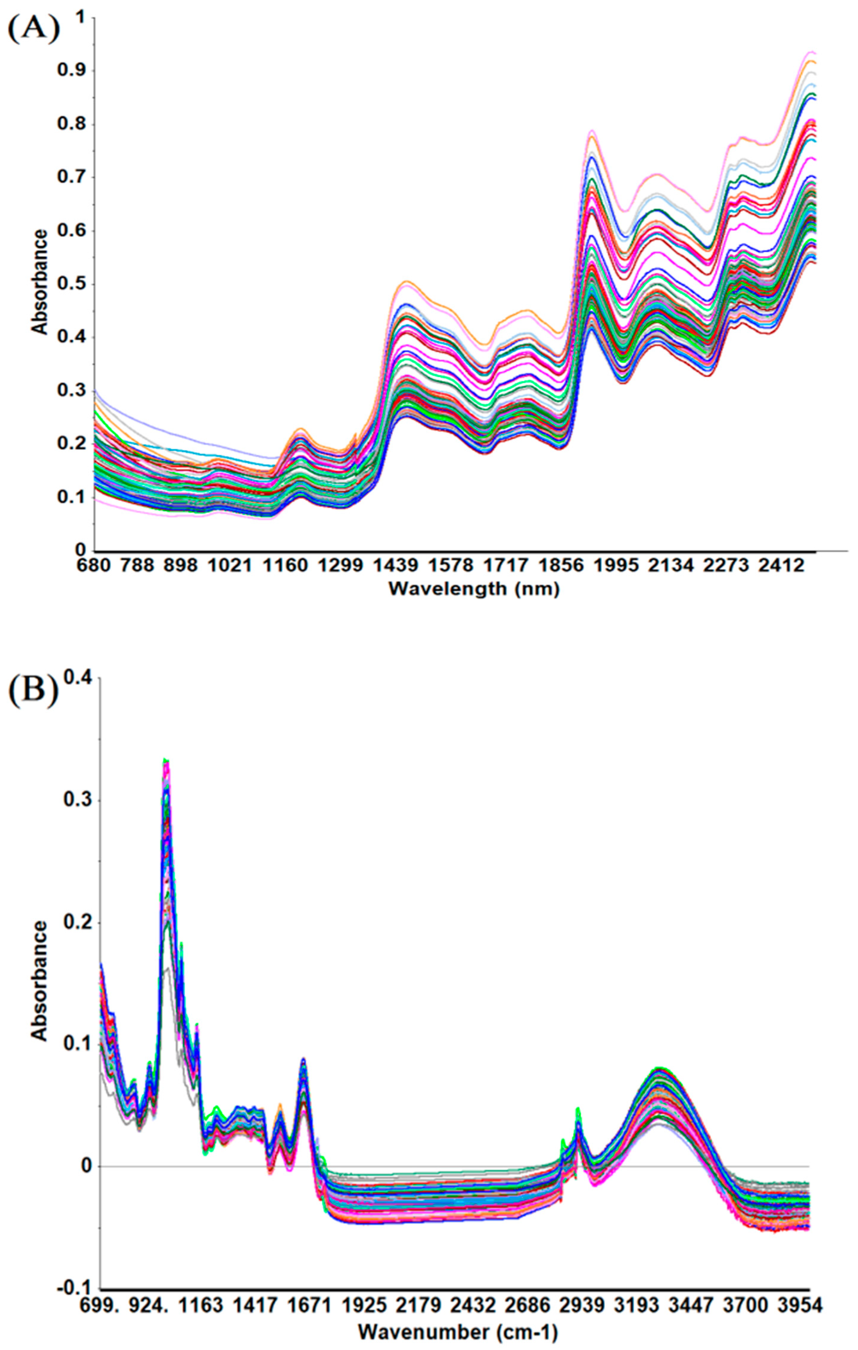
2.2. Overview of Spectral Data
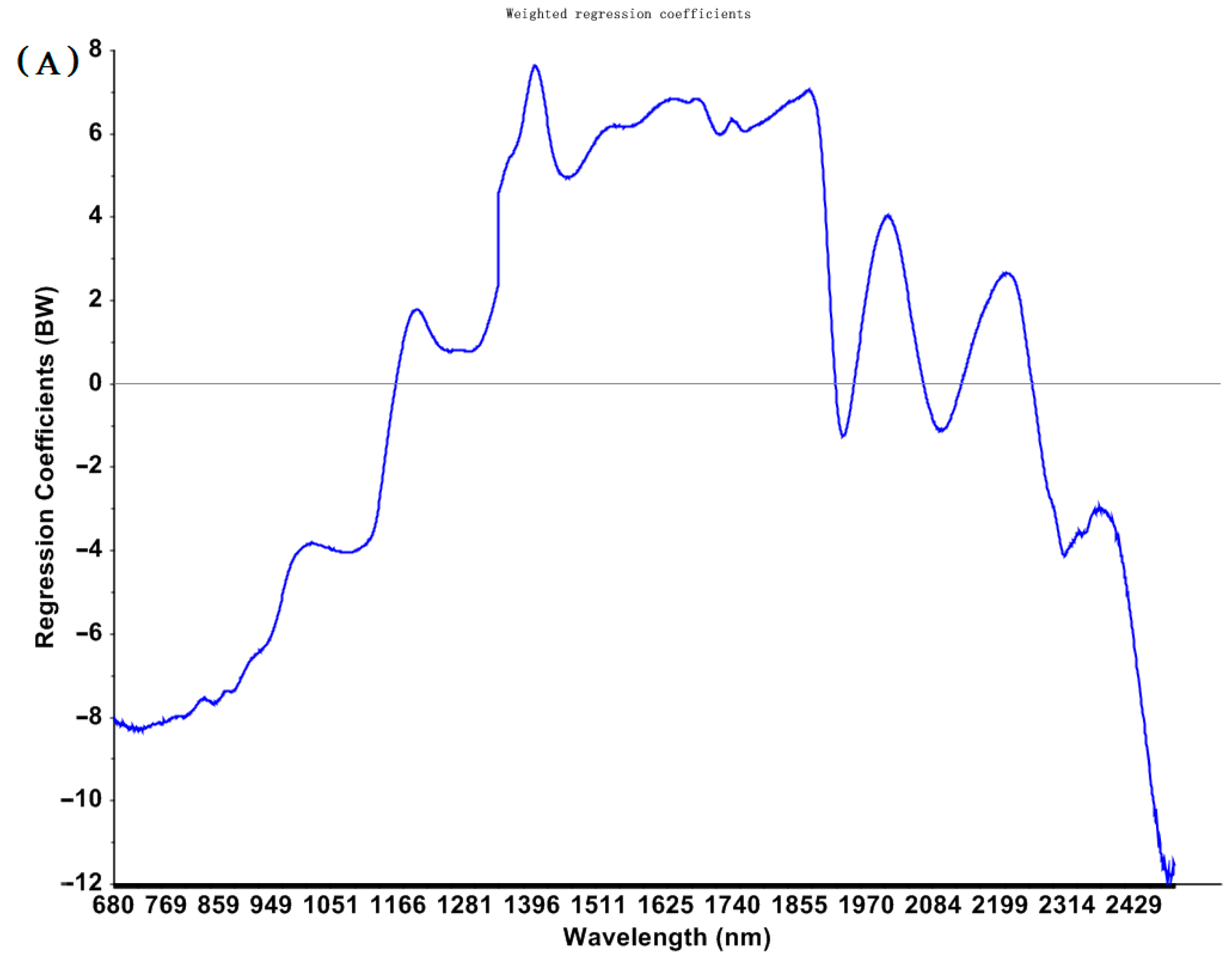
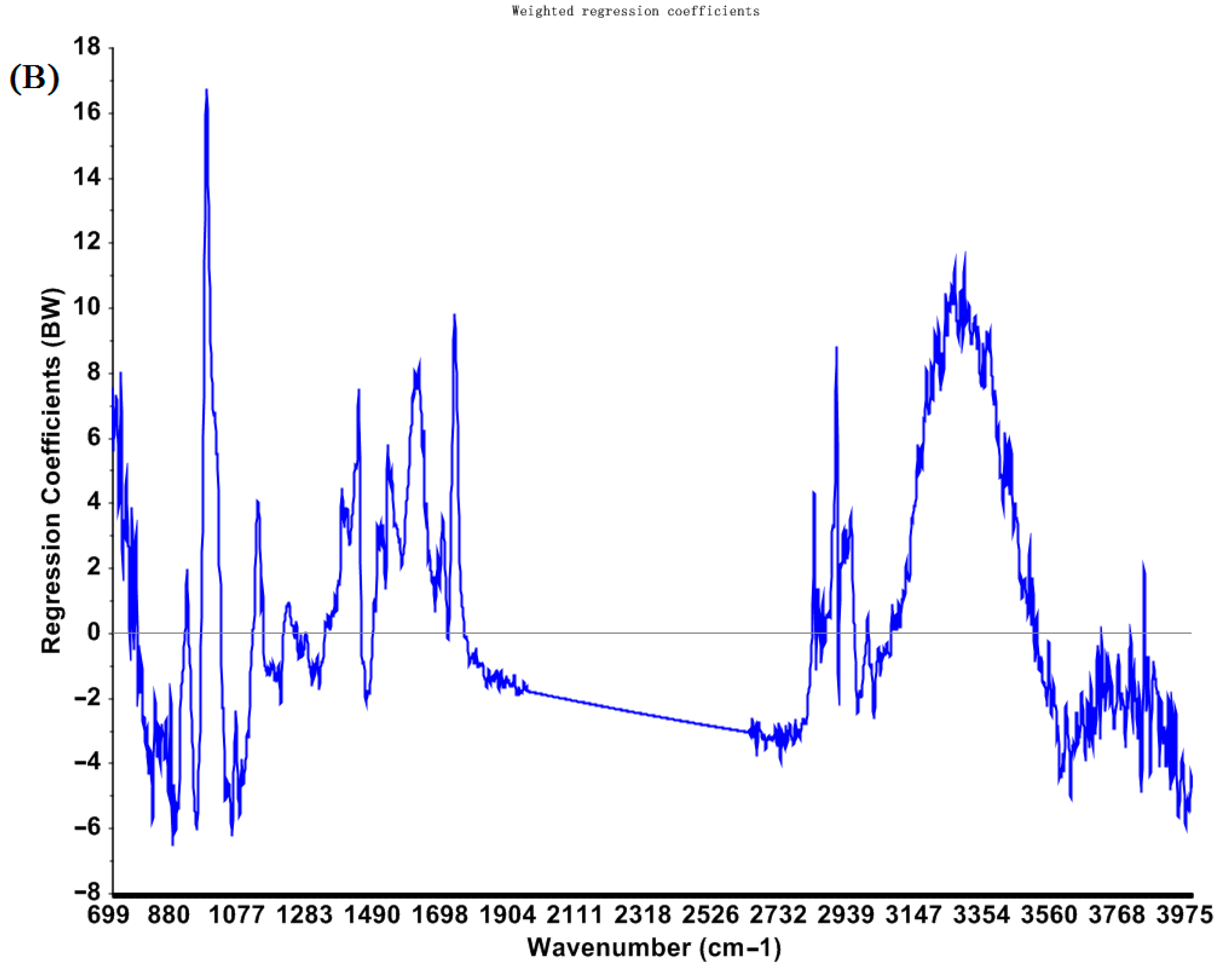
2.3. PLS Model Construction
2.4. Evaluation of PLS Models
3. Conclusions
4. Materials and Methods
4.1. Sample Preparation and LC-MS/MS Analysis
4.2. NIR and MIR Spectra Collection
4.3. Chemometric Analysis
Author Contributions
Funding
Institutional Review Board Statement
Informed Consent Statement
Data Availability Statement
Acknowledgments
Conflicts of Interest
Abbreviations
| General: | |
| ATR-FT/MIR | attenuated total reflectance-Fourier transform mid-infrared spectroscopy |
| CP | crude protein |
| EAs | ergot alkaloids |
| IR | infrared |
| MIR | mid-infrared |
| NIR | near-infrared |
| PCA | principal component analysis |
| PLS | partial least square |
| RC | Regression coefficient |
| RCA | Regression coefficient analysis |
| Spectral Pretreatment Technique: | |
| FD | first derivative |
| SNV | standard normal variate |
| FD-SNV | first derivative + SNV |
| MSC | multiplicative scattering correction |
| SNV-Detrending | SNV + detrending |
| SD-SNV | second derivative + SNV |
| SNV-SD | SNV + first derivative |
| Evaluate the models: | |
| R2C | determination for calibration |
| R2CV | coefficient of determination for cross-validation |
| R2P | coefficient of determination for prediction |
| SEC | standard error of calibration |
| SECV | standard error of cross-validation |
| SEP | standard error of prediction |
| RMSEC | root mean square error of calibration |
| RMSECV | root mean square error of cross-validation |
| RMSEP | root mean square error of prediction |
References
- Krska, R.; Stubbings, G.; Macarthur, R.; Crews, C. Simultaneous determination of six major ergot alkaloids and their epimers in cereals and foodstuffs by LC–MS–MS. Anal. Bioanal. Chem. 2008, 391, 563. [Google Scholar] [CrossRef] [PubMed]
- Vermeulen, P.; Pierna, J.F.; Van Egmond, H.P.; Zegers, J.; Dardenne, P.; Baeten, V. Validation and transferability study of a method based on near-infrared hyperspectral imaging for the detection and quantification of ergot bodies in cereals. Anal. Bioanal. Chem. 2013, 405, 7765–7772. [Google Scholar] [CrossRef] [PubMed]
- Schiff Jr, P.L. Ergot and its alkaloids. Am. J. Pharm. Educ. 2006, 70, 98. [Google Scholar] [CrossRef] [PubMed]
- Vermeulen, P.; Pierna, J.F.; Egmond, H.V.; Dardenne, P.; Baeten, V. Online detection and quantification of ergot bodies in cereals using near infrared hyperspectral imaging. Food Addit. Contam. Part A 2012, 29, 232–240. [Google Scholar] [CrossRef]
- Di Mavungu, J.D.; Malysheva, S.V.; Sanders, M.; Larionova, D.; Robbens, J.; Dubruel, P.; De Saeger, S. Development and validation of a new LC–MS/MS method for the simultaneous determination of six major ergot alkaloids and their corresponding epimers. Application to some food and feed commodities. Food Chem. 2012, 135, 292–303. [Google Scholar] [CrossRef]
- Tittlemier, S.A.; Drul, D.; Roscoe, M.; McKendry, T. Occurrence of ergot and ergot alkaloids in western Canadian wheat and other cereals. J. Agric. Food Chem. 2015, 63, 6644–6650. [Google Scholar] [CrossRef]
- Menzies, J.; Turkington, T. An overview of the ergot (Claviceps purpurea) issue in western Canada: Challenges and solutions. Can. J. Plant Pathol. 2015, 37, 40–51. [Google Scholar] [CrossRef]
- Coufal-Majewski, S.; Stanford, K.; McAllister, T.; Blakley, B.; McKinnon, J.; Chaves, A.V.; Wang, Y. Impacts of cereal ergot in food animal production. Front. Vet. Sci. 2016, 3, 15. [Google Scholar] [CrossRef]
- Shi, H.; Yu, P. Comparison of grating-based near-infrared (NIR) and Fourier transform mid-infrared (ATR-FT/MIR) spectroscopy based on spectral preprocessing and wavelength selection for the determination of crude protein and moisture content in wheat. Food Control 2017, 82, 57–65. [Google Scholar] [CrossRef]
- Shi, H.; Schwab, W.; Liu, N.; Yu, P. Major ergot alkaloids in naturally contaminated cool-season barley grain grown under a cold climate condition in western Canada, explored with near-infrared (NIR) and Fourier transform mid-infrared (ATR-FT/MIR) spectroscopy. Food Control 2019, 102, 221–230. [Google Scholar] [CrossRef]
- Hossain, M.; Goto, T. Near-and mid-infrared spectroscopy as efficient tools for detection of fungal and mycotoxin contamination in agricultural commodities. World Mycotoxin J. 2014, 7, 507–515. [Google Scholar] [CrossRef]
- Roberts, C.; Joost, R.; Rottinghaus, G. Quantification of ergovaline in tall fescue by near infrared reflectance spectroscopy. Crop Sci. 1997, 37, 281–284. [Google Scholar] [CrossRef]
- Gauglitz, G.; Vo-Dinh, T. Handbook of Spectroscopy; WILEY-VCH: Weinheim, Germany, 2003. [Google Scholar]
- Karoui, R.; Downey, G.; Blecker, C. Mid-infrared spectroscopy coupled with chemometrics: A tool for the analysis of intact food systems and the exploration of their molecular structure−Quality relationships—A review. Chem. Rev. 2010, 110, 6144–6168. [Google Scholar] [CrossRef] [PubMed]
- Manley, M. Near-infrared spectroscopy and hyperspectral imaging: Non-destructive analysis of biological materials. Chem. Soc. Rev. 2014, 43, 8200–8214. [Google Scholar] [CrossRef] [PubMed]
- Kong, J.; Yu, S. Fourier transform infrared spectroscopic analysis of protein secondary structures. Acta Biochim. Biophys. Sin. 2007, 39, 549–559. [Google Scholar] [CrossRef]
- Damiran, D.; Yu, P. Molecular basis of structural makeup of hulless barley in relation to rumen degradation kinetics and intestinal availability in dairy cattle: A novel approach. J. Dairy Sci. 2011, 94, 5151–5159. [Google Scholar] [CrossRef] [PubMed]
- Luypaert, J.; Heuerding, S.; Vander Heyden, Y.; Massart, D.L. The effect of preprocessing methods in reducing interfering variability from near-infrared measurements of creams. J. Pharm. Biomed. Anal. 2004, 36, 495–503. [Google Scholar] [CrossRef]
- Moros, J.; Garrigues, S.; de la Guardia, M. Vibrational spectroscopy provides a green tool for multi-component analysis. TrAC Trends Anal. Chem. 2010, 29, 578–591. [Google Scholar] [CrossRef]
- Hof, M. Basics of Optical Spectroscop. In Handbook of Spectroscopy; Gauglitz, G., Vo-Dinh, T., Eds.; Wiley-VCH: Weinheim, Germany, 2003. [Google Scholar]
- Grusie, T.; Cowan, V.; Singh, J.; McKinnon, J.; Blakley, B. Correlation and variability between weighing, counting and analytical methods to determine ergot (Claviceps purpurea) contamination of grain. World Mycotoxin J. 2017, 10, 209–218. [Google Scholar] [CrossRef]
- de Oliveira, G.A.; de Castilhos, F.; Renard, C.M.-G.C.; Bureau, S. Comparison of NIR and MIR spectroscopic methods for determination of individual sugars, organic acids and carotenoids in passion fruit. Food Res. Int. 2014, 60, 154–162. [Google Scholar] [CrossRef]
- Chun, H.; Keleş, S. Sparse partial least squares regression for simultaneous dimension reduction and variable selection. J. R. Stat. Soc. 2010, 72, 3–25. [Google Scholar] [CrossRef] [PubMed]
- Segtnan, V.H.; Isaksson, T. Evaluating near infrared techniques for quantitative analysis of carbohydrates in fruit juice model systems. J. Near Infrared Spectrosc. 2000, 8, 109–116. [Google Scholar] [CrossRef]
- Wold, S.; Trygg, J.; Berglund, A.; Antti, H. Some recent developments in PLS modeling. Chemom. Intell. Lab. Syst. 2001, 58, 131–150. [Google Scholar] [CrossRef]
- Nagelkerke, N.J. A note on a general definition of the coefficient of determination. Biometrika 1991, 78, 691–692. [Google Scholar] [CrossRef]
- Williams, P. Near-Infrared Technology—Getting the Best Out of Light; PDK Grain: Nanaimo, BC, Canada, 2003. [Google Scholar]
- Hell, J.; Prückler, M.; Danner, L.; Henniges, U.; Apprich, S.; Rosenau, T.; Kneifel, W.; Böhmdorfer, S. A comparison between near-infrared (NIR) and mid-infrared (ATR-FTIR) spectroscopy for the multivariate determination of compositional properties in wheat bran samples. Food Control 2016, 60, 365–369. [Google Scholar] [CrossRef]
- Roberts, C.; Benedict, H.; Hill, N.; Kallenbach, R.; Rottinghaus, G. Determination of ergot alkaloid content in tall fescue by near-infrared spectroscopy. Crop Sci. 2005, 45, 778–783. [Google Scholar] [CrossRef]
- Soto-Barajas, M.C.; Zabalgogeazcoa, I.; González-Martin, I.; Vázquez-de-Aldana, B.R. Qualitative and quantitative analysis of endophyte alkaloids in perennial ryegrass using near-infrared spectroscopy. J. Sci. Food Agric. 2017, 97, 5028–5036. [Google Scholar] [CrossRef]
- Dixit, Y.; Casado-Gavalda, M.P.; Cama-Moncunill, R.; Cama-Moncunill, X.; Jacoby, F.; Cullen, P.J.; Sullivan, C. Multipoint NIR spectrometry and collimated light for predicting the composition of meat samples with high standoff distances. J. Food Eng. 2016, 175, 58–64. [Google Scholar] [CrossRef]


| Parameter | Ergocornine | Ergocristine | Ergocryptine | Ergometrine | Ergosine | Ergotamine | Total EAs |
|---|---|---|---|---|---|---|---|
| N 1 | 37 | 64 | 53 | 45 | 36 | 44 | 75 |
| Mean, % | 97.48 | 743.31 | 142.07 | 150.59 | 56.88 | 337.48 | 1099.32 |
| Max, % | 1602.53 | 12,416.19 | 1954.23 | 1952.25 | 671.37 | 4462.75 | 21,970.40 |
| Min, % | 1.30 | 1.62 | 1.29 | 1.28 | 1.30 | 1.30 | 1.25 |
| Median, % | 5.63 | 39.26 | 11.30 | 11.20 | 7.07 | 33.21 | 42.10 |
| Range, % | 1601.23 | 12,414.57 | 1952.94 | 1950.97 | 670.07 | 4461.45 | 21,969.15 |
| Standard deviation, % | 296.89 | 1981.60 | 371.06 | 378.59 | 138.61 | 797.90 | 3221.62 |
| Variance, % | 88,142.30 | 3,927,756.00 | 137,686.30 | 143,327.80 | 19,212.86 | 636,637.90 | 10,378,850 |
| Skewness | 4.37 | 4.20 | 3.80 | 3.44 | 3.75 | 3.80 | 4.65 |
| 1 | ||||||||||||||
| Calibration | Cross-Validation | External Prediction | ||||||||||||
| Pretreatment | Technique | NC | NP | Wavelength Range | Factor | R2C | RMSEC | SEC | R2CV | RMSECV | SECV | R2P | RMSEP | SEP |
| NON | NIR | 24 | 12 | 1700–2500 nm | 1 | 0.02 | 350.35 | 357.89 | NA | 368.48 | 376.40 | − | − | − |
| MIR | 24 | 12 | 1800–700 cm−1 | 1 | 0.24 | 310.82 | 317.51 | NA | 407.52 | 415.97 | − | − | − | |
| Baseline offset | NIR | 24 | 12 | 680–2500 nm | 1 | 0.05 | 344.90 | 352.32 | NA | 370.36 | 378.32 | − | − | − |
| MIR | 24 | 12 | 1800–700 cm−1 | 1 | 0.17 | 324.02 | 330.99 | NA | 391.14 | 399.35 | − | − | − | |
| Detrending | NIR | 24 | 12 | 680–2500 nm | 1 | 0.05 | 344.95 | 352.37 | NA | 371.01 | 378.99 | − | − | − |
| MIR | 24 | 12 | 1800–700 cm−1 | 1 | 0.17 | 324.47 | 331.45 | NA | 398.61 | 407.06 | − | − | − | |
| MSC | NIR | 24 | 12 | 900–2000 nm | 1 | 0.07 | 341.07 | 348.41 | NA | 391.96 | 400.39 | − | − | − |
| MIR | 24 | 12 | 4000–700 cm−1 | 1 | 0.12 | 334.22 | 341.41 | NA | 410.75 | 419.58 | − | − | − | |
| SNV | NIR | 24 | 12 | 1700–2500 nm | 1 | 0.07 | 342.31 | 349.68 | NA | 381.52 | 389.72 | − | − | − |
| MIR | 24 | 12 | 4000–700 cm−1 | 1 | 0.12 | 334.14 | 341.33 | NA | 410.74 | 419.57 | − | − | − | |
| SNV-Detrending | NIR | 24 | 12 | 1100–2500 nm | 1 | 0.13 | 329.97 | 337.07 | NA | 399.26 | 407.80 | − | − | − |
| MIR | 24 | 12 | 3200–2700 cm−1 | 1 | 0.11 | 334.56 | 341.76 | NA | 415.97 | 424.91 | − | − | − | |
| FD | NIR | 24 | 12 | 1200–1900 nm | 1 | 0.04 | 347.05 | 354.52 | NA | 369.31 | 377.25 | − | − | − |
| MIR | 24 | 12 | 2750–2950 cm−1 | 1 | 0.10 | 336.55 | 343.79 | NA | 372.15 | 380.15 | − | − | − | |
| SD | NIR | 24 | 12 | 680–2500 nm | 4 | 0.92 | 100.16 | 102.31 | 0.12 | 345.48 | 352.30 | NA | 242.72 | 227.66 |
| MIR | 24 | 12 | 4000–700 cm−1 | 1 | 0.22 | 314.34 | 321.10 | NA | 383.78 | 392.03 | − | − | − | |
| FD-SNV | NIR | 24 | 12 | 680–2500 nm | 7 | 0.91 | 106.34 | 108.63 | 0.26 | 305.70 | 310.74 | NA | 275.39 | 271.23 |
| MIR | 24 | 12 | 4000–700 cm−1 | 1 | 0.29 | 299.40 | 305.84 | NA | 422.64 | 431.73 | − | − | − | |
| SD-SNV | NIR | 24 | 12 | 680–2500 nm | 3 | 0.74 | 181.33 | 185.23 | 0.14 | 341.38 | 348.60 | NA | 132.71 | 137.16 |
| MIR | 24 | 12 | 1800–700 cm−1 | 1 | 0.54 | 241.60 | 246.80 | NA | 408.13 | 416.85 | − | − | − | |
| 2 | ||||||||||||||
| Calibration | Cross-Validation | External Prediction | ||||||||||||
| Pretreatment | Technique | NC | NP | Wavelength Range | Factor | R2C | RMSEC | SEC | R2CV | RMSECV | SECV | R2P | RMSEP | SEP |
| NON | NIR | 24 | 12 | 1300–2500 nm | 1 | 0.04 | 1641.10 | 1676.39 | NA | 1843.45 | 1883.06 | − | − | − |
| MIR | 24 | 12 | 1800–700 cm−1 | 1 | 0.10 | 1607.24 | 1641.80 | NA | 1799.57 | 1838.15 | − | − | − | |
| Baseline offset | NIR | 24 | 12 | 1500–2500 nm | 1 | 0.04 | 1641.90 | 1677.21 | NA | 1844.92 | 1884.47 | − | − | − |
| MIR | 24 | 12 | 4000–700 cm−1 | 1 | 0.08 | 1621.82 | 1656.70 | 0.02 | 1749.88 | 1787.52 | NA | 1619.79 | 1686.22 | |
| Detrending | NIR | 24 | 12 | 680–2500 nm | 1 | 0.04 | 1644.06 | 1679.42 | NA | 1844.41 | 1883.88 | − | − | − |
| MIR | 24 | 12 | 1800–700 cm−1 | 1 | 0.11 | 1595.34 | 1629.65 | 0.05 | 1746.87 | 1784.41 | NA | 1652.37 | 1720.66 | |
| MSC | NIR | 24 | 12 | 1100–2300 nm | 1 | 0.05 | 1636.33 | 1671.52 | NA | 1773.05 | 1811.18 | − | − | − |
| MIR | 24 | 12 | 1800–700 cm−1 | 1 | 0.14 | 1572.20 | 1606.01 | NA | 1824.91 | 1864.11 | − | − | − | |
| SNV | NIR | 24 | 12 | 1300–2200 nm | 1 | 0.05 | 1636.02 | 1671.20 | NA | 1775.62 | 1813.81 | − | − | − |
| MIR | 24 | 12 | 1800–700 cm−1 | 1 | 0.14 | 1571.49 | 1605.29 | NA | 1825.58 | 1864.80 | − | − | − | |
| SNV-Detrending | NIR | 24 | 12 | 1100–2500 nm | 1 | 0.06 | 1627.35 | 1662.35 | NA | 1861.23 | 1901.21 | − | − | − |
| MIR | 24 | 12 | 1800–700 cm−1 | 1 | 0.15 | 1561.65 | 1595.24 | NA | 1838.60 | 1878.07 | − | − | − | |
| FD | NIR | 24 | 12 | 1250–2250 nm | 1 | 0.05 | 1639.82 | 1675.09 | NA | 1880.07 | 1920.31 | − | − | − |
| MIR | 24 | 12 | 4000–700 cm−1 | 1 | 0.14 | 1571.35 | 1605.15 | 0.01 | 1759.46 | 1797.30 | − | − | − | |
| SD | NIR | 24 | 12 | 1900–2500 nm | 5 | 0.99 | 173.13 | 176.85 | 0.14 | 1623.09 | 1657.99 | NA | 1868.90 | 1937.85 |
| MIR | 24 | 12 | 4000–700 cm−1 | 1 | 0.27 | 1447.99 | 1479.13 | NA | 1912.70 | 1953.59 | − | − | − | |
| FD-SNV | NIR | 24 | 12 | 680–2500 nm | 1 | 0.09 | 1597.72 | 1632.09 | NA | 1857.61 | 1897.39 | − | − | − |
| MIR | 24 | 12 | 4000–700 cm−1 | 1 | 0.18 | 1534.38 | 1567.38 | NA | 1853.50 | 1892.76 | − | − | − | |
| SD-SNV | NIR | 24 | 12 | 1250–2500 nm | 3 | 0.76 | 819.45 | 837.08 | 0.14 | 1610.93 | 1645.00 | 0.01 | 1547.16 | 1594.61 |
| MIR | 24 | 12 | 1800–700 cm−1 | 1 | 0.43 | 1281.08 | 1308.63 | NA | 2126.75 | 2165.27 | − | − | − | |
| 3 | ||||||||||||||
| Calibration | Cross-Validation | External Prediction | ||||||||||||
| Pretreatment | Technique | NC | NP | Wavelength Range | Factor | R2C | RMSEC | SEC | R2CV | RMSECV | SECV | R2P | RMSEP | SEP |
| NON | NIR | 31 | 15 | 1200–2500 nm | 1 | 0.03 | 364.82 | 368.85 | NA | 375.53 | 379.68 | − | − | − |
| MIR | 19 | 9 | 1800–700 cm−1 | 3 | 0.47 | 405.06 | 416.16 | 0.16 | 526.69 | 540.99 | NA | 691.37 | 545.08 | |
| Baseline offset | NIR | 31 | 15 | 1500–2500 nm | 1 | 0.07 | 347.99 | 353.74 | 0.02 | 373.01 | 379.18 | − | − | − |
| MIR | 19 | 9 | 1800–700 cm−1 | 1 | 0.35 | 448.32 | 460.60 | 0.12 | 533.11 | 547.52 | NA | 715.46 | 513.14 | |
| Detrending | NIR | 31 | 15 | 680–2500 nm | 1 | 0.06 | 348.59 | 354.35 | NA | 372.53 | 378.69 | − | − | − |
| MIR | 19 | 9 | 1800–700 cm−1 | 3 | 0.45 | 411.93 | 423.21 | 0.13 | 546.94 | 561.49 | NA | 575.98 | 505.01 | |
| MSC | NIR | 31 | 15 | 1700–2500 nm | 1 | 0.09 | 343.16 | 348.84 | NA | 384.04 | 390.39 | − | − | − |
| MIR | 19 | 9 | 1800–700 cm−1 | 3 | 0.49 | 398.18 | 409.09 | 0.20 | 521.37 | 535.26 | NA | 411.61 | 385.58 | |
| SNV | NIR | 31 | 15 | 1500–2400 nm | 1 | 0.10 | 342.20 | 347.86 | NA | 389.46 | 395.89 | − | − | − |
| MIR | 19 | 9 | 1800–700 cm−1 | 3 | 0.49 | 397.94 | 408.85 | 0.20 | 521.76 | 535.58 | NA | 408.38 | 382.90 | |
| SNV-Detrending | NIR | 31 | 15 | 900–2400 nm | 1 | 0.12 | 337.72 | 343.31 | NA | 389.16 | 395.57 | − | − | − |
| MIR | 19 | 9 | 1800–700 cm−1 | 3 | 0.47 | 402.38 | 413.40 | 0.22 | 500.03 | 513.66 | NA | 398.99 | 355.25 | |
| FD | NIR | 31 | 15 | 1300–2000 nm | 1 | 0.05 | 350.73 | 356.53 | 0.01 | 370.34 | 376.46 | − | − | − |
| MIR | 19 | 9 | 4000–700 cm−1 | 2 | 0.54 | 375.79 | 386.09 | 0.13 | 543.90 | 558.59 | NA | 491.24 | 295.8 | |
| SD | NIR | 31 | 15 | 1200–2500 nm | 1 | 0.03 | 353.81 | 359.66 | NA | 369.32 | 375.43 | − | − | − |
| MIR | 19 | 9 | 4000–700 cm−1 | 1 | 0.39 | 434.47 | 446.37 | 0.13 | 531.07 | 545.61 | NA | 518.52 | 273.73 | |
| FD-SNV | NIR | 31 | 15 | 680–2500 nm | 1 | 0.09 | 344.09 | 349.78 | NA | 376.95 | 383.18 | − | − | − |
| MIR | 19 | 9 | 4000–700 cm−1 | 2 | 0.59 | 355.49 | 365.23 | 0.21 | 515.21 | 528.67 | NA | 375.43 | 228.24 | |
| SD-SNV | NIR | 31 | 15 | 680–2500 nm | 1 | 0.03 | 354.04 | 359.89 | NA | 370.82 | 376.95 | − | − | − |
| MIR | 19 | 9 | 1800–700 cm−1 | 1 | 0.59 | 356.40 | 366.16 | 0.17 | 512.05 | 525.75 | NA | 488.11 | 313.50 | |
| 4 | ||||||||||||||
| Calibration | Cross-Validation | External Prediction | ||||||||||||
| Pretreatment | Technique | NC | NP | Wavelength Range | Factor | R2C | RMSEC | SEC | R2CV | RMSECV | SECV | R2P | RMSEP | SEP |
| NON | NIR | 26 | 12 | 1100–2500 nm | 1 | 0.04 | 436.89 | 445.54 | NA | 469.46 | 478.72 | − | − | − |
| MIR | 30 | 14 | 1800–700 cm−1 | 1 | 0.01 | 417.36 | 424.50 | NA | 459.18 | 467.02 | − | − | − | |
| Baseline offset | NIR | 26 | 12 | 1400–2500 nm | 1 | 0.06 | 432.42 | 440.98 | NA | 467.49 | 476.71 | − | − | − |
| MIR | 30 | 14 | 1800–700 cm−1 | 1 | 0.01 | 418.89 | 426.05 | NA | 447.97 | 455.58 | − | − | − | |
| Detrending | NIR | 26 | 12 | 1300–2000 nm | 1 | 0.06 | 431.64 | 440.19 | NA | 465.80 | 474.99 | − | − | − |
| MIR | 30 | 14 | 1800–700 cm−1 | 1 | 0.01 | 418.27 | 425.42 | NA | 452.58 | 460.30 | − | − | − | |
| MSC | NIR | 26 | 12 | 680–2500 nm | 1 | 0.05 | 434.55 | 443.16 | NA | 500.46 | 510.07 | − | − | − |
| MIR | 30 | 14 | 1800–700 cm−1 | 1 | 0.03 | 414.18 | 421.26 | NA | 466.45 | 474.42 | − | − | − | |
| SNV | NIR | 26 | 12 | 680–2500 nm | 1 | 0.05 | 434.58 | 443.19 | NA | 500.79 | 510.40 | − | − | − |
| MIR | 30 | 14 | 1800–700 cm−1 | 1 | 0.03 | 414.27 | 421.35 | NA | 466.12 | 474.09 | − | − | − | |
| SNV-Detrending | NIR | 26 | 12 | 1700–2400 nm | 1 | 0.03 | 437.83 | 446.50 | NA | 476.78 | 486.22 | − | − | − |
| MIR | 30 | 14 | 4000–700 cm−1 | 1 | 0.04 | 412.21 | 419.26 | NA | 475.95 | 484.05 | − | − | − | |
| FD | NIR | 26 | 12 | 1200–2000 nm | 1 | 0.07 | 430.40 | 438.93 | NA | 467.05 | 476.27 | − | − | − |
| MIR | 30 | 14 | 1800–700 cm−1 | 1 | 0.02 | 414.83 | 421.92 | NA | 464.67 | 472.49 | − | − | − | |
| SD | NIR | 26 | 12 | 680–2500 nm | 1 | 0.01 | 442.32 | 451.08 | NA | 465.11 | 474.32 | − | − | − |
| MIR | 30 | 14 | 1800–700 cm−1 | 1 | 0.18 | 379.45 | 385.94 | NA | 501.11 | 509.60 | − | − | − | |
| FD-SNV | NIR | 26 | 12 | 1200–2300 nm | 1 | 0.02 | 440.11 | 448.83 | NA | 467.84 | 477.11 | − | − | − |
| MIR | 30 | 14 | 4000–700 cm−1 | 1 | 0.12 | 392.88 | 399.60 | NA | 502.98 | 511.57 | − | − | − | |
| SD-SNV | NIR | 26 | 12 | 680–2500 nm | 2 | 0.62 | 275.62 | 281.08 | 0.16 | 415.20 | 423.08 | NA | 433.66 | 373.51 |
| MIR | 30 | 14 | 4000–700 cm−1 | 1 | 0.34 | 341.98 | 347.82 | NA | 508.91 | 517.61 | − | − | − | |
| 5 | ||||||||||||||
| Calibration | Cross-Validation | External Prediction | ||||||||||||
| Pretreatment | Technique | NC | NP | Wavelength Range | Factor | R2C | RMSEC | SEC | R2CV | RMSECV | SECV | R2P | RMSEP | SEP |
| NON | NIR | 22 | 10 | 680–2500 nm | 1 | 0.06 | 163.99 | 167.85 | NA | 175.88 | 180.02 | − | − | − |
| MIR | 24 | 10 | 4000–700 cm−1 | 1 | 0.06 | 157.93 | 161.32 | NA | 179.19 | 183.05 | − | − | − | |
| Baseline offset | NIR | 22 | 10 | 680–1900 nm | 1 | 0.08 | 162.35 | 166.17 | 0.02 | 175.07 | 179.18 | − | − | − |
| MIR | 24 | 10 | 1800–700 cm−1 | 1 | 0.08 | 156.78 | 160.15 | NA | 175.78 | 179.56 | − | − | − | |
| Detrending | NIR | 22 | 10 | 680–2500 nm | 1 | 0.07 | 163.14 | 166.98 | NA | 175.01 | 179.13 | − | − | − |
| MIR | 24 | 10 | 1800–700 cm−1 | 1 | 0.05 | 158.79 | 162.21 | NA | 180.67 | 184.55 | − | − | − | |
| MSC | NIR | 22 | 10 | 1400–2500 nm | 1 | 0.06 | 164.21 | 168.07 | NA | 180.45 | 184.69 | − | − | − |
| MIR | 24 | 10 | 1800–700 cm−1 | 1 | 0.04 | 160.23 | 163.68 | NA | 181.76 | 185.65 | − | − | − | |
| SNV | NIR | 22 | 10 | 1800–2500 nm | 1 | 0.06 | 163.72 | 167.58 | NA | 178.17 | 182.36 | − | − | − |
| MIR | 24 | 10 | 4000–700 cm−1 | 1 | 0.04 | 160.23 | 163.68 | NA | 183.52 | 187.46 | − | − | − | |
| SNV-Detrending | NIR | 22 | 10 | 1100–2500 nm | 1 | 0.09 | 161.30 | 165.10 | NA | 179.45 | 183.67 | − | − | − |
| MIR | 24 | 10 | 4000–700 cm−1 | 1 | 0.04 | 159.64 | 163.07 | NA | 184.87 | 188.83 | − | − | − | |
| FD | NIR | 22 | 10 | 1250–2050 nm | 1 | 0.07 | 163.42 | 167.26 | NA | 175.38 | 179.51 | − | − | − |
| MIR | 24 | 10 | 1800–700 cm−1 | 1 | 0.05 | 158.89 | 162.31 | NA | 184.74 | 188.67 | − | − | − | |
| SD | NIR | 22 | 10 | 1300–2500 nm | 1 | 0.06 | 164.25 | 168.12 | NA | 175.34 | 179.46 | − | − | − |
| MIR | 24 | 10 | 1800–700 cm−1 | 1 | 0.21 | 145.42 | 148.55 | NA | 183.62 | 187.16 | − | − | − | |
| FD-SNV | NIR | 22 | 10 | 1200–2500 nm | 1 | 0.06 | 163.68 | 167.54 | NA | 176.69 | 180.83 | − | − | − |
| MIR | 24 | 10 | 4000–700 cm−1 | 1 | 0.17 | 148.01 | 151.19 | NA | 201.63 | 205.69 | − | − | − | |
| SD-SNV | NIR | 22 | 10 | 680–2500 nm | 3 | 0.79 | 77.66 | 79.49 | 0.22 | 151.28 | 154.78 | NA | 83.43 | 87.43 |
| MIR | 24 | 10 | 4000–700 cm−1 | 1 | 0.43 | 123.63 | 126.29 | NA | 194.15 | 198.31 | − | − | − | |
| 6 | ||||||||||||||
| Calibration | Cross-Validation | External Prediction | ||||||||||||
| Pretreatment | Technique | NC | NP | Wavelength Range | Factor | R2C | RMSEC | SEC | R2CV | RMSECV | SECV | R2P | RMSEP | SEP |
| NON | NIR | 28 | 13 | 680–2500 nm | 1 | 0.02 | 915.72 | 932.52 | NA | 968.47 | 986.24 | − | − | − |
| MIR | 19 | 9 | 1800–700 cm−1 | 1 | 0.09 | 991.25 | 1018.41 | NA | 1065.90 | 1095.09 | − | − | − | |
| Baseline offset | NIR | 28 | 13 | 1400–2500 nm | 1 | 0.03 | 913.28 | 930.03 | NA | 965.59 | 983.31 | − | − | − |
| MIR | 19 | 9 | 4000–700 cm−1 | 1 | 0.07 | 1003.22 | 1030.71 | NA | 1079.52 | 1109.10 | − | − | − | |
| Detrending | NIR | 28 | 13 | 1200–2200 nm | 1 | 0.02 | 914.50 | 931.28 | NA | 964.52 | 982.22 | − | − | − |
| MIR | 19 | 9 | 1800–700 cm−1 | 1 | 0.08 | 997.38 | 1024.71 | 0.05 | 1069.46 | 1098.76 | − | − | − | |
| MSC | NIR | 28 | 13 | 1800–2400 nm | 1 | 0.02 | 916.84 | 933.67 | NA | 970.83 | 988.63 | − | − | − |
| MIR | 19 | 9 | 4000–700 cm−1 | 1 | 0.10 | 990.34 | 1017.48 | NA | 1086.01 | 1115.71 | − | − | − | |
| SNV | NIR | 28 | 13 | 1200–2500 nm | 1 | 0.02 | 917.60 | 934.43 | NA | 978.06 | 996.00 | − | − | − |
| MIR | 19 | 9 | 4000–700 cm−1 | 1 | 0.10 | 989.93 | 1017.05 | 0.02 | 1085.99 | 1115.69 | − | − | − | |
| SNV-Detrending | NIR | 28 | 13 | 680–2500 nm | 1 | 0.02 | 914.15 | 930.92 | NA | 964.86 | 982.57 | − | − | − |
| MIR | 19 | 9 | 4000–700 cm−1 | 1 | 0.10 | 985.34 | 1012.34 | 0.02 | 1088.02 | 1117.68 | − | − | − | |
| FD | NIR | 28 | 13 | 680–2500 nm | 1 | 0.03 | 913.61 | 930.18 | NA | 964.4 | 982.09 | − | − | − |
| MIR | 19 | 9 | 1800–700 cm−1 | 1 | 0.09 | 991.35 | 1018.52 | NA | 1075.01 | 1104.45 | − | − | − | |
| SD | NIR | 28 | 13 | 680–2500 nm | 1 | 0.02 | 914.46 | 931.24 | NA | 967.61 | 985.36 | − | − | − |
| MIR | 19 | 9 | 1800–700 cm−1 | 1 | 0.37 | 829.33 | 852.05 | NA | 1122.04 | 1152.23 | − | − | − | |
| FD-SNV | NIR | 28 | 13 | 1200–2400 nm | 1 | 0.02 | 914.74 | 931.52 | NA | 970.03 | 987.77 | − | − | − |
| MIR | 19 | 9 | 4000–700 cm−1 | 1 | 0.15 | 961.67 | 987.67 | NA | 1134.22 | 1164.78 | − | − | − | |
| SD-SNV | NIR | 28 | 13 | 1200–2500 nm | 1 | 0.02 | 914.79 | 931.58 | NA | 967.85 | 985.60 | − | − | − |
| MIR | 19 | 9 | 1800–700 cm−1 | 1 | 0.41 | 796.51 | 818.34 | NA | 1180.58 | 1210.74 | − | − | − | |
| 7 | ||||||||||||||
| Calibration | Cross-Validation | External Prediction | ||||||||||||
| Pretreatment | Technique | NC | NP | Wavelength Range | Factor | R2C | RMSEC | SEC | R2CV | RMSECV | SECV | R2P | RMSEP | SEP |
| NON | NIR | 32 | 15 | 1500–2500 nm | 1 | 0.01 | 2178.57 | 2213.43 | NA | 2377.60 | 2415.63 | − | − | − |
| MIR | 32 | 16 | 1800–700 cm−1 | 1 | 0.09 | 1422.66 | 1445.42 | NA | 1731.73 | 1758.91 | − | − | − | |
| Baseline offset | NIR | 32 | 15 | 1400–2500 nm | 1 | 0.02 | 2169.78 | 2204.50 | NA | 2359.29 | 2397.03 | − | − | − |
| MIR | 32 | 16 | 1800–700 cm−1 | 1 | 0.01 | 1484.59 | 1508.35 | NA | 1563.29 | 1588.30 | − | − | − | |
| Detrending | NIR | 32 | 15 | 680–2500 nm | 1 | 0.02 | 2174.16 | 2208.95 | NA | 2360.68 | 2398.44 | − | − | − |
| MIR | 32 | 16 | 1800–700 cm−1 | 1 | 0.02 | 1476.51 | 1500.13 | NA | 1653.27 | 1679.72 | − | − | − | |
| MSC | NIR | 32 | 15 | 1000–2400 nm | 1 | 0.05 | 2142.26 | 2176.53 | NA | 2276.78 | 2313.21 | − | − | − |
| MIR | 32 | 16 | 1800–700 cm−1 | 1 | 0.04 | 1466.07 | 1489.52 | NA | 1798.71 | 1827.05 | − | − | − | |
| SNV | NIR | 32 | 15 | 1000–2500 nm | 1 | 0.05 | 2142.06 | 2176.34 | NA | 2271.13 | 2307.42 | − | − | − |
| MIR | 32 | 16 | 1800–700 cm−1 | 1 | 0.04 | 1463.25 | 1486.66 | NA | 1797.76 | 1825.54 | − | − | − | |
| SNV-Detrending | NIR | 32 | 15 | 1200–2400 nm | 1 | 0.07 | 2114.08 | 2147.91 | NA | 2398.58 | 2436.79 | − | − | − |
| MIR | 32 | 16 | 1800–700 cm−1 | 1 | 0.06 | 1449.47 | 1472.66 | NA | 1871.50 | 1901.40 | − | − | − | |
| FD | NIR | 32 | 15 | 1000–2300 nm | 1 | 0.02 | 2174.77 | 2209.56 | NA | 2380.40 | 2418.48 | − | − | − |
| MIR | 32 | 16 | 4000–700 cm−1 | 1 | 0.09 | 1423.08 | 1445.85 | NA | 1795.95 | 1823.84 | − | − | − | |
| SD | NIR | 32 | 15 | 680–2500 nm | 1 | 0.01 | 2188.35 | 2223.37 | NA | 2373.48 | 2411.46 | − | − | − |
| MIR | 32 | 16 | 1800–700 cm−1 | 1 | 0.39 | 1163.46 | 1182.07 | NA | 1978.47 | 2006.52 | − | − | − | |
| FD-SNV | NIR | 32 | 15 | 1000–2000 nm | 1 | 0.06 | 2126.02 | 2160.04 | NA | 2367.78 | 2405.55 | − | − | − |
| MIR | 32 | 16 | 1800–700 cm−1 | 1 | 0.25 | 1298.58 | 1319.36 | NA | 1932.25 | 1961.22 | − | − | − | |
| SD-SNV | NIR | 32 | 15 | 1200–2500 nm | 5 | 0.96 | 427.97 | 434.82 | 0.14 | 2099.56 | 2131.14 | 0.22 | 1585.45 | 1582.25 |
| MIR | 32 | 16 | 1800–700 cm−1 | 1 | 0.28 | 1268.08 | 1288.37 | NA | 1797.17 | 1825.61 | − | − | − | |
Disclaimer/Publisher’s Note: The statements, opinions and data contained in all publications are solely those of the individual author(s) and contributor(s) and not of MDPI and/or the editor(s). MDPI and/or the editor(s) disclaim responsibility for any injury to people or property resulting from any ideas, methods, instructions or products referred to in the content. |
© 2023 by the authors. Licensee MDPI, Basel, Switzerland. This article is an open access article distributed under the terms and conditions of the Creative Commons Attribution (CC BY) license (https://creativecommons.org/licenses/by/4.0/).
Share and Cite
Shi, H.; Yu, P. Using Molecular Spectroscopic Techniques (NIR and ATR-FT/MIR) Coupling with Various Chemometrics to Test Possibility to Reveal Chemical and Molecular Response of Cool-Season Adapted Wheat Grain to Ergot Alkaloids. Toxins 2023, 15, 151. https://doi.org/10.3390/toxins15020151
Shi H, Yu P. Using Molecular Spectroscopic Techniques (NIR and ATR-FT/MIR) Coupling with Various Chemometrics to Test Possibility to Reveal Chemical and Molecular Response of Cool-Season Adapted Wheat Grain to Ergot Alkaloids. Toxins. 2023; 15(2):151. https://doi.org/10.3390/toxins15020151
Chicago/Turabian StyleShi, Haitao, and Peiqiang Yu. 2023. "Using Molecular Spectroscopic Techniques (NIR and ATR-FT/MIR) Coupling with Various Chemometrics to Test Possibility to Reveal Chemical and Molecular Response of Cool-Season Adapted Wheat Grain to Ergot Alkaloids" Toxins 15, no. 2: 151. https://doi.org/10.3390/toxins15020151