1. Introduction
Hyperspectral remote sensing image (HSI) classification is the process of attempting to allocate class labels to pixels within a set of hyperspectral images utilizing classification methods. It represents a primary application of hyperspectral remote sensing data and is a crucial technique for interpreting and analyzing HSIs [
1].
Through years of research and exploration, numerous scholars have proposed an exceedingly diverse array of classification methods. Depending on the availability of class knowledge, the classification methods are classified as unsupervised, supervised, or semi-supervised learning approaches [
2]. Unsupervised methods rely solely on the intrinsic separability of the data and include clustering algorithms such as K-Means [
3], spectral clustering [
4], Fuzzy C-Means (FCM) [
5], hierarchical clustering [
6], and density-based spatial clustering (DBSCAN) [
7].
Supervised methods, using labeled samples for training, generally achieve better performance. Common supervised approaches include probability-based methods, kernel transformations, random forests, and sparse representation [
1].
Semi-supervised learning methods can be categorized into generative and discriminative models. Generative models establish joint probability distribution between classes, reflecting similarity within the same class. Examples include a Markov random field (MRF) model incorporating spatial and spectral features [
8] and the S
2MLR (Soft sparse multinomial logistic regression) model [
9]. Discriminative models directly learn conditional probability distributions, such as a graph-based framework describing the importance of labeled samples [
10] and a transductive SVM method [
11] implementing a weighting strategy for unlabeled samples. These methods enhance classification by leveraging both labeled and unlabeled data for improved performance.
In recent years, deep convolutional neural networks (CNNs) have achieved tremendous success in various tasks on natural images and have also quickly garnered significant attention from the hyperspectral remote sensing image-processing community [
12,
13]. Another highly significant representational learning model in deep learning is the generative adversarial networks (GANs), first proposed by Goodfellow and colleagues in 2014 [
14]. This network combines the characteristics of both generative and discriminative models. Subsequently, a variety of GAN-based models have been continuously introduced [
15,
16,
17], leading to a series of semi-supervised and unsupervised learning methods based on GANs [
18]. For instance, Springenberg proposed Cat-GAN in 2015 [
19], which is capable of handling image classification tasks and generating samples. This method offers an approach to learning discriminative classifiers from unlabeled or partially labeled data. In 2016, Odena et al. introduced Semi-GAN [
20], which forces the discriminative model to output
labels (where
k represents the number of classes) to perform semi-supervised classification. He and co-authors presented a semi-supervised method for hyperspectral images based on GANs named 3DBF-GANs [
21], which learns and classifies hyperspectral images after extracting spatial–spectral features using three-dimensional bilateral filtering. In 2023, Zhan et al. proposed a hyperspectral image semi-supervised classification method based on a one-dimensional GAN network with spectral angle distance (SADGAN), achieving commendable performance with limited labeled samples [
22].
Due to the inherent phenomena of “same material different spectrum” and “different material same spectrum” in hyperspectral images [
23], solely relying on spectral information is insufficient for the effective identification of ground objects. Simultaneously, pixels within hyperspectral images tend to belong to the same category as adjacent pixels with a high probability, forming the foundation for classification methods based on spatial features. Many scholars have proposed joint classification studies combining spectral and spatial features on this theoretical basis [
24].
According to the literature summary [
23], the spatial–spectral classification framework for hyperspectral images typically follows a series of steps. First, spectral and spatial features are extracted from the data. Then, these features are either selected or fused together. The selected or fused features are subsequently inputted into a classifier for the purpose of classification. Finally, spatial regularization is performed using spatial features to enhance the classification results. Depending on the stage at which the fusion of spectral and spatial information occurs, spatial–spectral classification methods can be categorized into three types [
25]: preprocessing-based classification [
26], integrated classification [
27,
28], and postprocessing-based classification [
29,
30].
In the preprocessing-based spatial–spectral classification of hyperspectral images, spatial-feature-extraction methods targeted at neighborhood pixels are commonly employed due to the converging characteristics between pixels and their surrounding neighborhoods [
25]. Techniques based on Markov random fields [
31], spectral correlation [
32], morphological features [
33], and superpixel segmentation [
34] are prevalent in this context.
The utilization of filtering techniques for spatial feature extraction in preprocessing-based classification is garnering increasing attention from researchers. Commonly used filtering-based methods include the approach proposed by Bau et al. [
35], which is based on Gabor filtering. This method extracts features such as orientation, scale, and wavelength of hyperspectral images through three-dimensional Gabor filtering. Another method, proposed by Chen et al. [
36], combines Gabor filtering with CNNs techniques. It employs Gabor filters for edge and texture feature extraction and, when combined with convolutional filters, can mitigate the issue of model overfitting.
At present, researchers predominantly employ filtering-based methods to extract spatial features [
35,
36], particularly the Guided Image Filter (GIF) proposed by He et al. [
37], which has demonstrated promising results in hyperspectral image classification [
38,
39,
40,
41].
GIF operates based on the Local Linear Model, computing the filter output by considering the content of the guidance image, enabling image smoothing while preserving edges. However, while GIF can guide the filtering output by referencing the information of a guidance image, it overlooks the structural inconsistency between the reference signal and the target signal captured under different conditions, failing to adequately retain image edges in complex image structures. Recently, Guo et al. proposed the mutually guided image filter (muGIF) algorithm [
42], which employs the concept of relative structure to measure the similarity between the reference image and the target image. A global optimization objective is designed on this basis to achieve high-quality image filtering.
Inspired by this, we propose a hyperspectral image classification model based on the muGIF algorithm in this paper. Initially, considering the two-dimensional spatial features and one-dimensional spectral features inherent in hyperspectral images, a spatial feature extraction method based on mutually guided image filtering and band-distance-grouped principal component is proposed. This method groups bands according to the band distance in hyperspectral images, extracting the principal components of each group of band subsets as the guidance map for the current band subset to carry out mutually guided image filtering. Subsequently, deep CNN- and GAN-classification models are constructed for the filtered hyperspectral images, selecting training samples for classifier training and performing spatial–spectral classification of the hyperspectral images.
The main contributions of this paper are as follows.
(1) Proposing a hyperspectral image classification model based on the muGIF algorithm. This model takes into account the two-dimensional spatial features and one-dimensional spectral features inherent in hyperspectral images.
(2) Introducing a spatial feature extraction method based on mutually guided image filtering and a band-distance-grouped principal component. This method groups bands according to the band distance in hyperspectral images, extracting the principal components of each group of band subsets as the guidance map for the current band subset to carry out mutually guided image filtering.
The rest of the paper is organized as follows.
Section 2 describes the proposed muGIF-based classification method in detail.
Section 3 describes the data sets used for the comparison experiments and the specific settings of the comparison methods in the experiments.
Section 4 reports the results of the experiments and the related analysis. Conclusions are presented in
Section 5.
2. Methodology
In this paper, a hyperspectral image-classification method based on mutually guided image filtering is proposed. On this basis, the filtered images are classified by combining deep learning models such as CNN and GAN.
Figure 1 describes the framework of the spatial–spectral classification method of muGIF and deep learning. Firstly, the original hyperspectral image is grouped based on band distance density, and principal component analysis is performed on each group of images after grouping. Each group extracts a principal component as the guided image of that group of band images; then, the muGIF filtering algorithm is used to filter all bands in each group of images; finally, the filtered data set is trained through CNN models or GAN models to obtain the corresponding classifiers for classification.
Section 2.1 explains how muGIF works.
Section 2.2 provides an overview of how the proposed methods in this paper work.
Section 2.2.1 explains how to perform muGIF filtering after obtaining grouped principal components through band distance density. On this basis,
Section 2.2.2 and
Section 2.2.3 present classification methods combining mutual conductive image filtering with CNNs and GANs, respectively.
2.1. Mutually Guided Image Filtering
Image filtering can generally be divided into two categories: frequency domain filtering and spatial filtering. Spatial filtering, in particular, is a technique employed to modify or enhance images according to specific rules. It can typically be formulated as follows:
and denote the input and output signals respectively, represents the fidelity term, signifies the regularization term of the output, and is a non-negative coefficient balancing these two terms.
To better utilize the information from the guided image and reflect the corresponding structural relationship between the reference image
and target image
, the relative structure of
with respect to
is defined as follows [
42]:
where
i denotes a pixel on the image (
x,
y) and
represents a first-order derivative filter comprising both the horizontal (
h) and vertical (
v) directions. The relative structure
measures the structural difference of
with respect to
.
With the definition of relative structure, the optimization objective for muGIF can be constructed as follows:
, , , and are non-negative constants used to balance the corresponding terms; denotes the norm, and are employed to constrain and not to deviate too much from and .
Directly solving the aforementioned optimization problem is quite challenging. Guo et al. proposed an approximate solution method [
42]: initially finding an approximate substitute for the relative structure
:
Herein,
and
are introduced to avoid division-by-zero errors. The corresponding optimization objective can be replaced with the following form:
where
,
,
and
are the vector forms of
,
,
and
respectively. Let
and
(
) represent the diagonal matrices of the
ith diagonal element
and
respectively. Correspondingly, the objective Function (
5) is transformed into
Herein,
is the Toeplitz matrix of the discrete gradient operator in the
d direction. Equation (
6) can be solved through Alternating Least Squares (ALS) to obtain the output after muGIF filtering
2.2. Mutually Guided Image Filtering for Hyperspectral Images Classification
2.2.1. Principal Components of Band Distance Density
Similar to the GIF algorithm, the muGIF algorithm also requires a guidance image as a reference to filter the target image. According to the concept of relative structure described in Equation (
2), when the guidance image
is in the edge region, the first-order gradient is larger. Hence, the penalty term
for
is relatively more minor, achieving the effect of preserving boundaries. Conversely, when the guidance image
is in a smooth region with a smaller first-order gradient, the penalty term is relatively larger, resulting in a more pronounced smoothing effect. Therefore, the choice of the guidance image is of significant importance to the filtering effect of the muGIF algorithm.
In spatial–spectral classification methods of hyperspectral images using guided image filtering, the primary components obtained from PCA decomposition of all band images are usually used as the guidance images for filtering:
where
represents the hyperspectral image data,
) denotes the PCA decomposition of
using principal component analysis [
43,
44], and
indicates the
ith principal component, and
n represents the number of bands.
Researchers often choose the first or the first three principal components as the guidance image for filtering [
38,
40,
41].
However, since hyperspectral images often contain multiple bands, and there is a significant difference between different bands, using one or a few principal components simultaneously as the guidance image for multiple bands cannot provide a good filtering reference for different band images, which can easily lead to information distortion. This paper proposes a principal component-extraction method based on band distance density to address this question. By grouping all bands according to band distance density, one principal component is extracted for each group, and this principal component is used as the guidance image for filtering all band images in this group.
Band distance can be used to describe the sparsity level of features between bands:
where
n is the total number of bands and
is the spectral response value of the
ith band. The equation represents that
is the absolute value of the difference between the
ith and the
i + 1th adjacent bands. From the Equation (
10), we can derive that the total distance between all adjacent bands in the hyperspectral image is
where
j represents the pixel in the hyperspectral image. Next, the entire band needs to be divided into
p subgroups. Let
,
be the band number of the ending position of the
kth group, and let
denote the number of bands in each group. Then, we have
and
By sequentially solving Equation (
14) from top to bottom, we can determine the specific values of
and thus obtain the specific division of the
p subintervals.
Once the partitioning of each group in the hyperspectral image is established, we can perform PCA decomposition on all bands of each group:
represents the PCA decomposition of the data set
composed of bands from the
kth group. Finally, the first principal component
obtained after decomposition for each group is used as the guide image for the muGIF filtering of that group:
where
represents the image of the
ith band, and
is the corresponding output image after the muGIF filtering. All the filtered images corresponding to the bands are then reassembled into a new data set
, which is subsequently involved in the classification process.
2.2.2. Classification Algorithm Based on MuGIF and CNN with Spectral Angle Distance
After obtaining the data set
that the algorithm above has filtered, a classifier can be employed to categorize this data set. In this context, the convolutional neural network is chosen as the classifier. We select training data for the training process, and ultimately, the model with the highest accuracy is picked as the final classifier for classification. This algorithm is named muGIF-CNN in this paper, as detailed in Algorithm 1.
| Algorithm 1: muGIF-CNN |
- 1:
Data: Hyperspectral datas et - 2:
Result: Classifier CNN - 3:
Initialize group count p, CNN training epochs , training sample ratio - 4:
Determine the starting position of each band grouping based on Equation ( 14) - 5:
Decompose each band group separately using PCA according to Equation ( 15), obtaining the first principal component of each group as the guide image - 6:
Use different guide images for different band groups, compute the filtered image for each band image based on Equation ( 16), and assemble them into the new data set - 7:
Extract training samples from the hyperspectral data based on the training sample ratio - 8:
for do - 9:
Train the CNN model using the training samples - 10:
Update the weights of the CNN using the gradient descent algorithm - 11:
Update ; - 12:
end for - 13:
After training, save the model CNN with the highest accuracy and output;
|
2.2.3. Classification Algorithm Based on MuGIF and GAN with Spectral Angle Distance
Similarly, we choose the SADGAN algorithm [
22], combined with muGIF filtering, which will implement the spatial–spectral joint classification of hyperspectral images in a semi-supervised manner. This algorithm is named muGIF-SADGAN in this paper, and the specific description of the algorithm is shown in Algorithm 2.
| Algorithm 2: muGIF-SADGAN |
- 1:
Data: Hyperspectral data set - 2:
Result: Classifier finetuning CNN(FTCNN) - 3:
Initialize group number p, SADGAN training epochs , FTCNN training epochs , extracted convolutional layer feature depth , training sample proportion - 4:
Calculate the starting position of each band grouping according to Equation ( 14) - 5:
Use PCA to decompose each band group separately based on Equation ( 15), and obtain the first principal component of each group as the guidance image - 6:
Calculate the filtered image of each band based on Equation ( 16). Use different guidance images for different band groups and form the new data set - 7:
for do - 8:
Acquire m generated samples and m real samples - 9:
Feed both the generated and real data into model D of SADGAN for training and update the weights of D using gradient ascent - 10:
Take m noise samples and feed them into model G of SADGAN for training, update the weights of G using gradient descent - 11:
Update ; - 12:
end for - 13:
After training, save models G and D - 14:
Select training samples from the hyperspectral data according to the proportion - 15:
Feed the training samples into model D, then extract features from convolutional layers, flatten them, and concatenate them as inputs for CNN - 16:
for do - 17:
Train the FTCNN with the fused features of training samples - 18:
Update the weights of FTCNN using the gradient descent algorithm - 19:
Update ; - 20:
end for - 21:
After training, save and output the model with the highest accuracy
|
3. Datasets and Experimental Setting
This section discusses the details of the data sets chosen for the experiments and the setup of the various methods used in the experiments for comparison with the methods we propose.
3.1. Data Sets Description
To validate the effectiveness of the proposed muGIF-CNN and muGIF-SADGAN methods, we conducted comparative experiments on the Indian Pines, Pavia University, Salinas Valley, and Tianshan data sets. The first three datasets are widely used datasets used to validate the proposed method, and Tianshan is an actual application data set. We extracted 5%, 0.5%, 0.5%, and 10% of the data from them, respectively, as training data (further divided into training and validation data sets at an 8:2 ratio), with the remaining samples constituting the testing data set.
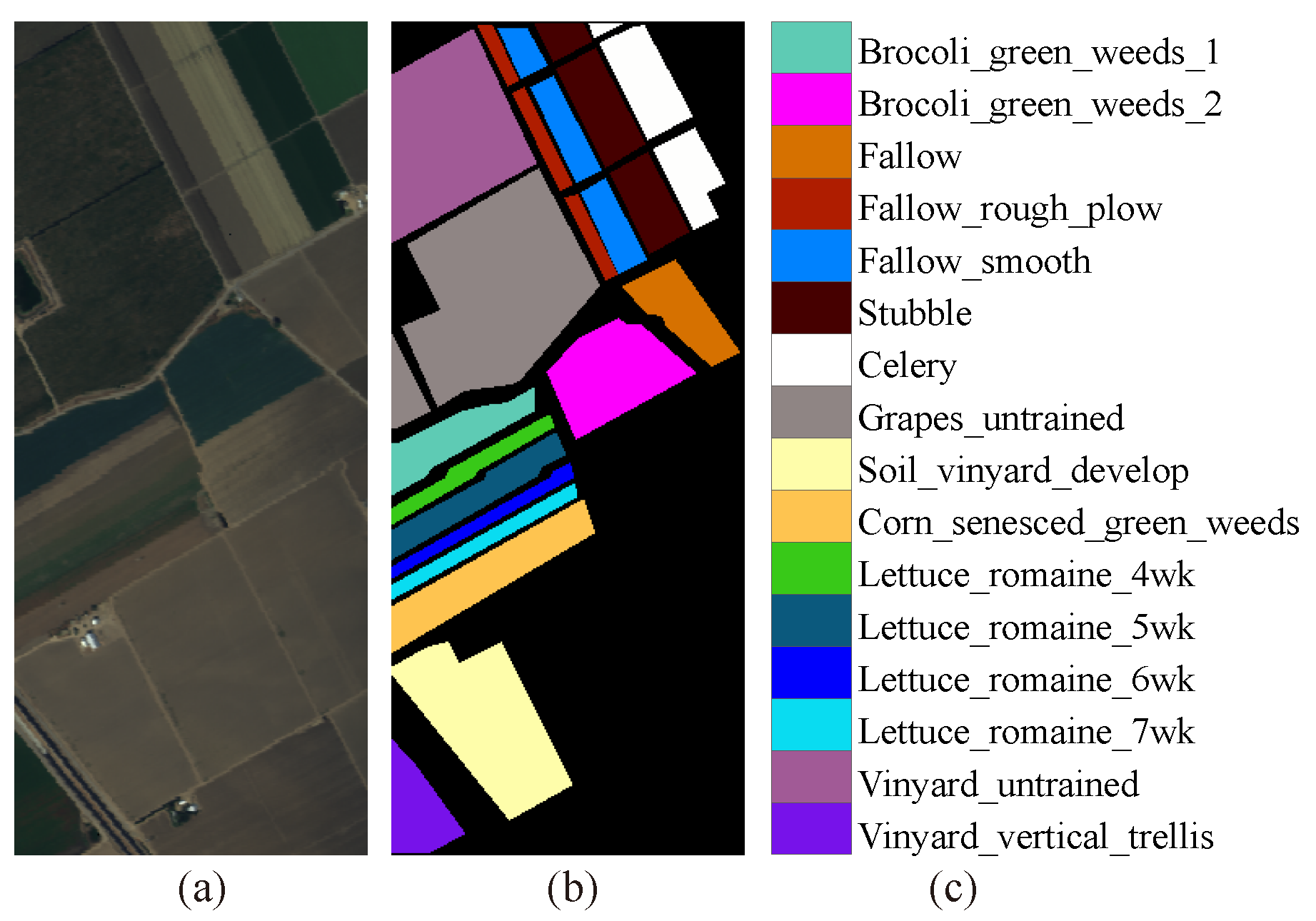
The first hyperspectral data set utilized in this study is the Indian Pines data set, which was acquired in 1992 using the airborne visible/infrared imaging spectrometer (AVIRIS) sensor over the Indian Pines region in northwestern Indiana. The image consists of
pixels and encompasses 220 spectral bands, covering a wavelength range from 400 to 2200 nm with a fine spectral resolution. The spatial resolution of the image is approximately 20 m. Prior to the experiments, bands affected by water absorption and noise were eliminated, resulting in a data set comprising 200 bands. For our experiments, we employed a total of 10,249 pixels representing sixteen distinct classes.
Figure 2 showcases the color composite of the Indian Pines image alongside the corresponding ground truth data.
The second data set used in this study was captured by the airborne Reflective Optics System Imaging Spectrometer (ROSIS) sensor over the urban area of the University of Pavia, located in northern Italy, in 2002. The image has dimensions of
pixels. It possesses a high spatial resolution of 1.3 m and covers a spectral range from 430 to 860 nm. The acquired image consists of 103 bands. In total, there are 42,776 samples across nine distinct categories.
Figure 3 displays the color composite of the Pavia University image along with the corresponding ground truth data.
The third data set was collected by the AVIRIS sensor over Salinas Valley in southern California, USA, in 1998. The image size is
pixels, the coverage is 400 to 2500 nm, and the spatial resolution is 3.7 m. After the noisy and water absorption bands were removed, the number of bands in the acquired image was 204. There are a total of 54,129 samples, including 16 classes.
Figure 4 shows the color composite of the Salinas image and the corresponding ground truth data.
The fourth data set used in this study is the airborne HyMap data collected over Tianshan, China. The HyMap imaging spectrometer operates within a spectral range of 400–2480 nm. The spectral bandwidth of the data is not fixed and typically falls between 15 nm and 18 nm, with an average bandwidth of approximately 16 nm. The data set possesses a spatial resolution of 9 m and a pixel resolution of
. The spectral response values of the features span from 1 to 10,000. The experimental data were subjected to atmospheric and geometric correction. After removing bands affected by water absorption and noise, the data set was reduced to 123 bands.
Figure 5a represents the color composite map of the Tianshan data. Based on the existing local geological map, the reference data are depicted in
Figure 5b.
Figure 5c provides the name of each class, accompanied by the color legend.
Table 1 presents the sample sizes for the Indian Pines, Pavia University, Salinas, and Tianshan data sets. The Tianshan data set has a large number of data and small inter-class differences, which significantly differ from the first three datasets. This difference can verify the applicability of the proposed method on different sensor datasets in the experiments. This disparity also implies that the computational processing time for the same algorithm will be longer when applied to the Tianshan data set. To mitigate this issue, we employed a band selection algorithm to downscale the Tianshan data set, thereby reducing the processing time for subsequent experiments.
Figure 6 depicts the average spectral curves for each class within the four data sets mentioned. A notable observation is that the Tianshan data set showcases smoother intra-class spectral features and smaller inter-class differences when compared to the other publicly available data sets. This suggests that the Tianshan data set exhibits relatively limited variations between different classes of geologic bodies. Consequently, classification algorithms employed for this data set must possess enhanced performance to effectively differentiate between the various classes and facilitate efficient geologic mapping.
Moreover, obtaining corresponding training samples for hyperspectral images, particularly in geologic mapping regions characterized by complex environments, presents significant challenges. Therefore, reducing reliance on labeled samples in classification becomes crucial. To address this challenge, in addition to a supervised classification approach, we also adopt a semi-supervised classification approach utilizing GANs for spectral classification and the muGIF algorithm for spatial–spectral classification.
3.2. Methods of Comparison and Experimental Setup
Methods compared with muGIF-CNN and muGIF-SADGAN include 1DCNN, EMP-SVM, GIF-FSAE, Gabor-CNN, SSGAT, and GIF-CNN, where those with CNN indicate that the method uses the convolutional neural network as the classifier. Unless expressly noted, relevant parameters in the methods are determined through five-fold cross-validation in the experiments.
Details of the setup of these methods in the experiment are described below:
(1) 1DCNN [
45]: The method 1DCNN employs a one-dimensional deep convolutional neural network to classify spectral features. For consistency in comparison standards, unless otherwise specified, other methods in this experiment that use CNN as a classifier all adopt the structure of 1DCNN.
(2) EMP-SVM [
33]: For the method, several principal components of the hyperspectral image are first extracted using the principal component analysis (PCA) method (four principal components in this experiment). Subsequently, the EMP algorithm is employed to extract spatial–spectral features, with a window radius size of 4. We performed four opening and closing operations on each principal component, resulting in
spatial–spectral features derived from the four principal component images. Finally, we employed the Support Vector Machine (SVM) to classify these features.
(3) GIF-FSAE [
46]: This is a method for hyperspectral image classification that combines guided image filtering and sparse autoencoders, integrating unsupervised and supervised feature learning. Initially, the raw hyperspectral image undergoes PCA decomposition. On one hand, the first three principal components are used as guide images, while on the other, the initial 30 principal components are stacked to serve as input images. Guided image filtering utilizes two window radius sizes for spatial feature extraction. These spatial features are then fused with spectral features and introduced to the sparse autoencoder for model training.
(4) Gabor-CNN [
36]: This method combines Gabor filtering with CNNs. Initially, spatial features are extracted from the three principal components obtained through PCA decomposition of the hyperspectral image using Gabor filters. These Gabor filters consist of four different orientations. The resulting spatial features are then stacked together to form a new data set, which is subsequently fed into the CNN for training.
(5) SSGAT: The SSGAT method [
47] utilizes the aggregation of features from both labeled and unlabeled samples by computing attention coefficients between a node and its neighboring nodes. This approach effectively combines spectral and spatial information from all the samples. In this experiment, the weight parameters of the SSGAT method were optimized using the Adam optimizer. The learning rate was set to 0.01, and the number of training epochs was set to 300.
(6) GIF-CNN: The GIF-CNN method [
41] is a hyperspectral image classification approach that combines multi-scale guided image filtering with CNNs.
(7) muGIF-CNN-1PC: This is a method proposed in this paper for hyperspectral image classification based on mutually guided image filtering and CNNs, using the first principal component as the guide image. As defined in Equation (
5), the muGIF algorithm itself comprises six parameters:
,
,
,
,
,
. Among them,
and
are utilized to prevent division-by-zero errors and are set to
in this paper. As indicated by Equations (
7) and (
8), the performance of muGIF is determined by
and
. Initially, we set
and
, thus only considering the parameters
and
. According to Equation (
6),
and
influence the input image and the guide image, respectively. Larger values result in smoother output images. Since our emphasis is on filtering the input image, we only consider the setting of the
parameter. The specific value of
is determined through five-fold cross-validation, and in our experiments, we set
.
(8) muGIF-CNN: In the muGIF-CNN method, the guiding image is obtained using a band distance grouping method. For each data set, the bands are divided into five groups. Each band group undergoes PCA decomposition, and the first principal component is selected as the guiding image for filtering that particular band group. The remaining parameters and settings of muGIF-CNN are consistent with the muGIF-CNN-1PC method.
(9) muGIF-SADGAN: Another hyperspectral image-classification method proposed in this paper is muGIF-SADGAN. This method combines mutually guided image filtering with the SADGAN algorithm [
22]. The parameters used for muGIF in muGIF-SADGAN are consistent with those of the muGIF-CNN-1PC method.
The experimental hardware environment for this section consisted of an Intel Core i5-4590 3.3 GHz CPU, 20 GB of RAM, and a TitanX GPU. The computer operating system used was Ubuntu 16.04. The algorithms were developed using TensorFlow, the Keras deep learning library, and the Scikit-learn machine learning library. To quantitatively evaluate the experimental results, the confusion matrix was utilized as the basis. Key performance metrics such as Overall Accuracy (OA), Average Accuracy (AA), and the kappa coefficient (%) were calculated to compare the classification performance of different methods.
4. Experimental Results and Analysis
This section discusses the classification results of various comparative methods discussed in the
Section 3 and the proposed methods on four datasets. Finally, an analysis and discussion are conducted on the impact of muGIF parameters’ settings on the classification results.
4.1. Experimental Results for the Indian Pines Data Set
Table 2 presents the Overall Accuracy (OA), Average Accuracy (AA), and kappa coefficient
(%) achieved by different comparison methods on the Indian Pines data set. For this evaluation, 5% of the samples from each class were randomly selected as training samples. Additionally,
Figure 7 showcases the classification results obtained by each method. The experimental findings clearly demonstrate the superior performance of the methods proposed in this paper, which are based on the combination of muGIF and deep learning, for spatial–spectral classification of hyperspectral images.
From
Table 2, it is evident that methods integrating both spatial and spectral features exhibit significant improvements compared to the 1DCNN method, which relies solely on spectral features for classification. This indicates that models incorporating both spatial and spectral features are better suited for the spatial–spectral characteristics of hyperspectral images. Furthermore, deep-learning-based algorithms outperform the traditional classic spatial–spectral classification algorithm EMP-SVM, achieving higher accuracy. Specifically, the proposed muGIF-CNN and muGIF-SADGAN methods in this paper show an improvement of 8.53% and 9.55% in Overall Accuracy (OA) compared to EMP-SVM, respectively.
Methods such as Gabor-CNN and guided-image-based methods (GIF-FSAE, GIF-CNN, muGIF-CNN-1PC, muGIF-CNN, muGIF-SADGAN), thanks to their edge-preserving effect, generally outperform EMP-based methods. Among these, muGIF-based methods have an edge over GIF-based methods as muGIF can handle different structures between the guided image and target image separately, leading to better edge preservation and homogenous area smoothing. Consequently, methods based on muGIF demonstrate superior classification accuracy. Specifically, compared to GIF-CNN methods, the muGIF-CNN-1PC method achieves an increase in OA of 0.34%, the muGIF-CNN method improves by 1.15%, and the muGIF-SADGAN method improves by 2.17%. Compared to the latest SSGAT method, muGIF-CNN-1PC, with only the first principal component, has mediocre performance, but muGIF-CNN and muGIF-SADGAN also achieve better classification results.
The muGIF-CNN method, which utilizes band distance grouping to obtain multiple principal components as guided images, shows a slight increase in accuracy compared to the muGIF-CNN-1PC method, which uses a single principal component as a guiding image. This suggests that guiding with grouped principal components is beneficial for feature extraction. Additionally, muGIF-SADGAN, which learns features from unlabeled samples in a semi-supervised manner, achieves slightly higher classification accuracy compared to muGIF-CNN. However, it is worth noting that as the spatial feature extraction of muGIF becomes more refined, the difference between semi-supervised and supervised classification methods becomes narrower.
Referring to the classification results depicted in
Figure 7, it is evident that the muGIF-CNN-1PC, muGIF-CNN, and muGIF-SADGAN methods exhibit fewer noisy points compared to other classification methods. This observation highlights the notable filtering effect of the muGIF algorithm prior to classification. Specifically, when comparing the central region of
Figure 7h–j, it becomes apparent that the muGIF-CNN and muGIF-SADGAN methods accurately identify class 2 objects surrounded by class 11 objects. This implies that utilizing the first principal component as the guiding image in muGIF-CNN-1PC results in excessive information loss from the original bands. In contrast, the muGIF-CNN and muGIF-SADGAN methods, which employ band distance grouping principal components as guiding images for each band group, can better preserve useful information during the filtering process, consequently enhancing classification accuracy.
4.2. Experimental Results for the Pavia University Data Set
Table 3 presents the overall classification accuracy (OA), average classification accuracy (AA), and kappa coefficient
(%) achieved by different comparison methods on the Pavia University data set. For this evaluation, 0.5% of samples from each class were randomly selected as training samples. Additionally,
Figure 8 showcases the classification result maps obtained using each method. The experimental findings unequivocally demonstrate the superior performance of the proposed muGIF-CNN and muGIF-SADGAN methods in the spatial–spectral classification of hyperspectral images.
Table 3 reveals that the performance of different methods on the Pavia University data set is similar to that on the Indian Pines data set. Notably, the 1DCNN method, relying solely on spectral features, exhibits significantly lower performance compared to methods integrating spatial–spectral features. The proposed muGIF-CNN and muGIF-SADGAN methods achieve improvements of 5.55% and 6.24% in OA accuracy, respectively, when compared to EMP-SVM.
Methods utilizing guided images, such as Gabor-CNN and those based on guided image filtering (GIF-FSAE, GIF-CNN, muGIF-CNN-1PC, muGIF-CNN, and muGIF-SADGAN), generally outperform EMP-SVM methods due to their edge-preserving effect. Among these, the muGIF-CNN and muGIF-SADGAN methods demonstrate notable advantages over GIF filtering methods GIF-FSAE and GIF-CNN.
The accuracy of the muGIF-CNN-1PC method, which uses the first principal component as a guiding image, is 1.22% lower than that of the muGIF-CNN method, which adopts band distance grouping principal components. Meanwhile, the semi-supervised muGIF-SADGAN method exhibits slightly higher accuracy than the muGIF-CNN and SSGAT.
Figure 8 shows that, similarly to the classification result maps on the Indian Pines data set, the muGIF-based methods do not exhibit as many noisy points as other classification methods. This observation further emphasizes the significant smoothing effect of muGIF prior to the classification process.
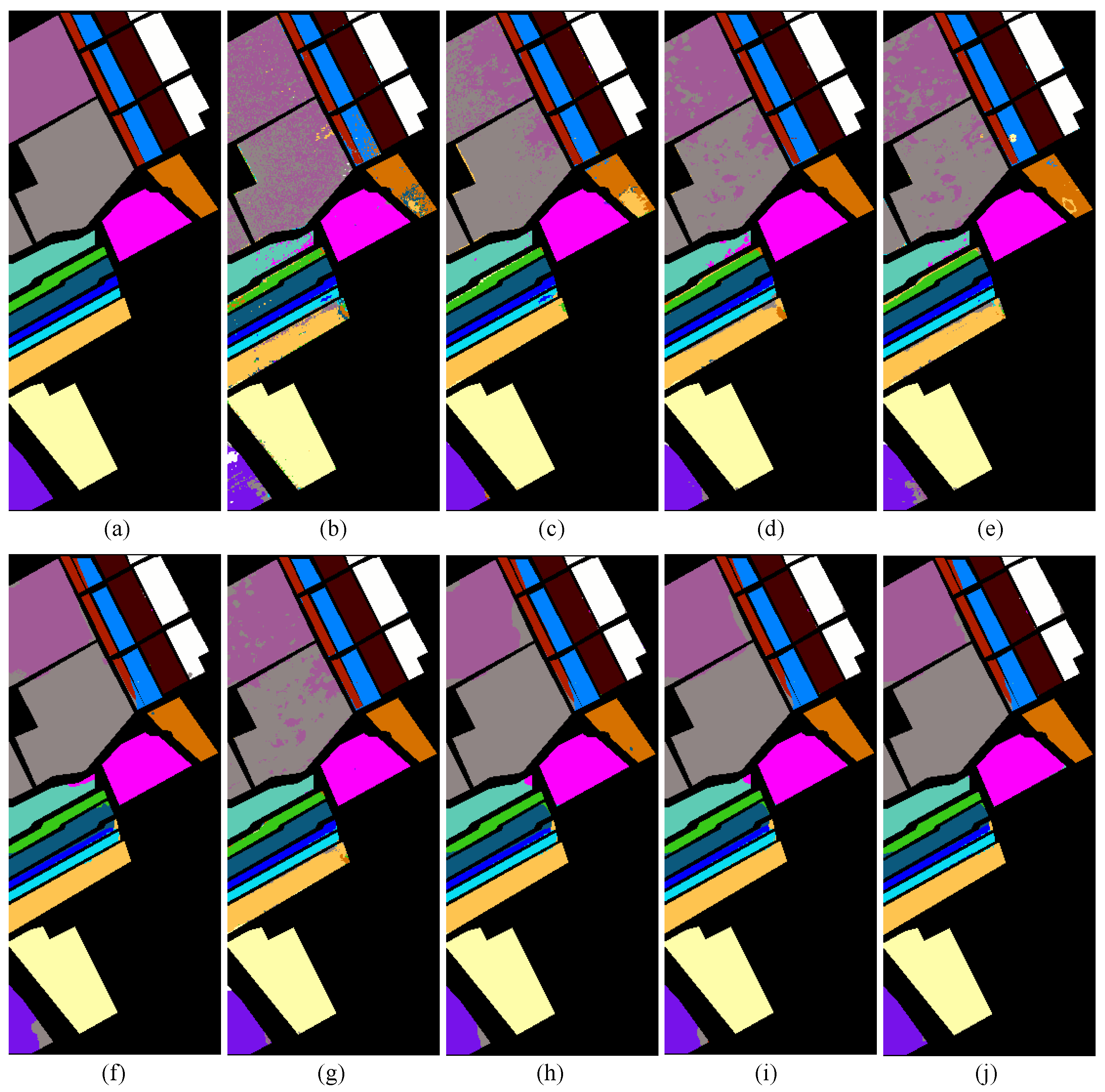
4.3. Experimental Results for the Salinas Valley Data Set
Table 4 presents the overall classification accuracy (OA), average classification accuracy (AA), and kappa coefficient
(%) achieved by different comparison methods on the Salinas Valley data set. For this evaluation, 0.5% of samples from each class were randomly selected as training samples. Additionally,
Figure 9 showcases the classification result maps obtained using each method. Consistent with the experiments conducted on the previous two data sets, the results once again highlight the superior performance of the proposed muGIF-CNN and muGIF-SADGAN methods in the spatial–spectral classification of hyperspectral images.
Table 4 reveals that the classification accuracy of the 1DCNN method, which relies solely on spectral features, is generally lower compared to methods incorporating spatial–spectral features. The OA accuracy of the proposed muGIF-CNN and muGIF-SADGAN methods surpasses that of EMP-SVM by 6.98% and 7.98%, respectively. Furthermore, when compared to GIF-based method GIF-FSAE, the muGIF-SADGAN method demonstrates improvements in OA accuracy by 4.92%.
Furthermore, as depicted in
Figure 9, both the muGIF-CNN and muGIF-SADGAN methods exhibit exceptional performance, achieving desirable accuracy results even with limited labeled samples. Notably, the result maps generated by these methods are free of excessive noise points.
4.4. Experimental Results for the Tianshan Data Set
The Tianshan data set offers insights into the classification characteristics of hyperspectral remote sensing specifically in geological bodies, setting it apart from the previous three hyperspectral data sets that focused on agriculture. In the experiments, we aim to evaluate various algorithms for classifying geological bodies in hyperspectral images, highlighting their performance in applications of the real-world classification of geological bodies.
For the task of hyperspectral image classification, we have selected several algorithms, namely SVM [
33], 1DCNN [
45], HSGAN [
48], and SADGAN [
22]. These algorithms primarily focus on spectral classification.
In addition to these spectral algorithms, we have also employed the SVM-EMP [
33], GIF-CNN [
41], SSGAT [
47], muGIF-CNN, and muGIF-SADGAN algorithms for spatial–spectral classification. These algorithms incorporate both spectral and spatial information for enhanced classification accuracy.
Table 5 provides a comparison of the classification performances of various methods using only 10% of the training data. Upon analyzing the classification results of the first four spectral classification methods, it is observed that, among the deep learning methods, namely 1DCNN, HSGAN, and SADGAN, the semi-supervised learning methods HSGAN and SADGAN, which effectively utilize both labeled and unlabeled samples, outperform the 1DCNN method.
In terms of spatial–spectral joint classification, the non-deep-learning traditional classification method SVM-EMP leverages spatial features. However, its Overall Accuracy lags behind that of other deep learning-based spatial–spectral classification methods and is even slightly lower than that of the spectral-only classification method SADGAN.
Benefiting from the excellent filtering properties of muGIF, the muGIF-CNN method outperforms GIF-CNN and SSGAT, showcasing improvements in OA accuracy of 2.40% and 1.34%, respectively. The superior performance of muGIF-CNN highlights the effectiveness of muGIF in enhancing classification accuracy in comparison to other methods.
Additionally, the Kruskal–Wallis test [
49] was used to analyze the statistical significance of differences in performance obtained by the different methods being compared. The results of the Kruskal–Wallis test are a test statistic value and a
p-value. The test statistic indicates the degree of difference between the results, and the
p-value represents the probability of obtaining such a difference by chance alone, assuming the null hypothesis is true.
The p-value obtained from the test of the eight methods in this experiment is , which is significantly lower than the significance level of 0.05. This indicates a substantial difference in the median performance among the methods used in the experimental comparisons. Therefore, we can confidently conclude that the comparison methods are statistically distinct and can serve as reliable benchmarks for evaluating the performance of image classification.
Figure 10 showcases the maps comparing the classification results obtained from the experiments conducted on the Tianshan data set. In these experiments, 50 bands were selected as the final data set using the BSCNN band selection method [
50].
The classification result maps of SADGAN, which benefit from the generator-generated (augmented) samples and multilayer convolutional features provided by GAN, demonstrate more detailed information. However, it is noticeable that many cluttered spots are present in homogeneous regions, as this method does not utilize spatial features.
Upon analyzing the classification results of the GIF-CNN, SSGAT, muGIF-CNN, and muGIF-SADGAN methods, it becomes evident that the integration of a spatial feature-extraction method aids in correctly categorizing most of the clutter in homogeneous regions, unlike SADGAN. This observation highlights the importance of incorporating spatial features in achieving accurate classification results.
Indeed, it is crucial to acknowledge that the ground truth data, although manually created, may still contain errors and uncertainties. These errors can impact the evaluation of classification methods and introduce challenges in accurately assessing their performance.
While spectral classification methods, such as 1DCNN and SADGAN, often exhibit lower accuracy compared to spatial–spectral joint classification methods, they have the advantage of providing a more detailed representation of ground features. These spectral methods can capture fine spectral variations and subtle differences in the data, resulting in a more granular classification output.
On the other hand, spatial–spectral joint classification algorithms tend to smooth out homogeneous regions by leveraging spatial information. This smoothing effect can potentially lead to the loss of some detailed information present in these regions.
To gain meaningful insights and perform a comprehensive analysis, it is recommended to conduct simultaneous spectral-based classification and spatial–spectral joint classification on the same hyperspectral image data within the same region. By comparing the classification results obtained from both approaches, a more holistic understanding of the data can be achieved, taking into account the strengths and limitations of each method.
4.5. Influence of Mutually Guided Image-Filtering Parameters
Figure 11 depicts the influence of variation in the parameter
on image filtering in muGIF-CNN. In
Figure 11a, the original image of the 95th band of the Indian Pines data set is presented. As the value of
steadily increases, it becomes apparent that the original image progressively becomes smoother or more blurred.
Figure 12 demonstrates the influence of the
parameter on the final classification results of the Indian Pines data set. To clearly illustrate its impact on the classification performance, the
x-axis in the graph is presented on a logarithmic scale.
From
Figure 11 and
Figure 12, it can be inferred that, for hyperspectral image classification, the gradual smoothing of images while preserving edges is beneficial for extracting spatial features. This process helps to enhance the representation of spatial information in the classification task. However, it is important to note that excessive smoothing can cause hyperspectral image samples to converge, ultimately affecting the overall classification performance.
In the comparative experiment conducted in this paper, a value of
corresponds to the filtering effect depicted in
Figure 11f. At this specific parameter setting, the edge portions in the original image are well preserved, while the interior becomes as smooth as possible. This optimal balance between smoothing and edge preservation results in the highest classification accuracy among the different parameter values tested.
These findings highlight the significance of selecting an appropriate value for the parameter in muGIF-CNN. It is crucial to strike a balance between smoothing and edge preservation to achieve the best classification performance for hyperspectral images.
5. Conclusions
In this study, we propose a method for HSI spatial feature extraction based on a muGIF and combined with the band-distance-grouped principal component, which aims to fully exploit the spatial–spectral features of hyperspectral images and enhance their classification performance.
The method extracts the principal components of hyperspectral image band groups based on band distance and uses them as guided images for the muGIF algorithm. Each band group of the hyperspectral image is individually filtered to extract spatial features from the data. Finally, deep learning models, specifically CNNs and GANs, are employed to classify the filtered hyperspectral images.
The key innovation of our approach lies in the application of muGIF with gouping principal components in hyperspectral image classification. Unlike traditional methods that use a single principal component as the guided image, we introduce a novel approach for principal-component segmentation extraction based on band-distance density. This method enriches the theoretical content of hyperspectral image spatial filtering, leading to improved classification results.
Experimental results demonstrate that our proposed muGIF-based approach effectively extracts the spatial–spectral joint features of hyperspectral images, thereby elevating the classification accuracy of hyperspectral imagery. Comparative evaluations against conventional techniques and several recently popular spatial–spectral classification methods validate the superior performance of muGIF-CNN and muGIF-SADGAN.


