Article

H-RNet: Hybrid Relation Network for Few-Shot Learning-Based Hyperspectral Image Classification

1
School of Data Science and Engineering, Guangdong Polytechnic Normal University, Guangzhou 510630, China
2
Academy of Heyuan, Guangdong Polytechnic Normal University, Heyuan 517099, China
3
School of Computer Science, Guangdong Polytechnic Normal University, Guangzhou 510630, China
4
Guangdong Provincial Key Laboratory of Intellectual Property and Big Data, Guangdong Polytechnic Normal University, Guangzhou 510665, China
5
National Subsea Centre, Robert Gordon University, Aberdeen AB21 0BH, UK
*
Author to whom correspondence should be addressed.
Remote Sens. 2023, 15(10), 2497; https://doi.org/10.3390/rs15102497
Submission received: 18 March 2023 / Revised: 29 April 2023 / Accepted: 5 May 2023 / Published: 9 May 2023

Abstract

:
Deep network models rely on sufficient training samples to perform reasonably well, which has inevitably constrained their application in classification of hyperspectral images (HSIs) due to the limited availability of labeled data. To tackle this particular challenge, we propose a hybrid relation network, H-RNet, by combining three-dimensional (3-D) convolution neural networks (CNN) and two-dimensional (2-D) CNN to extract the spectral–spatial features whilst reducing the complexity of the network. In an end-to-end relation learning module, the sample pairing approach can effectively alleviate the problem of few labeled samples and learn correlations between samples more accurately for more effective classification. Experimental results on three publicly available datasets have fully demonstrated the superior performance of the proposed model in comparison to a few state-of-the-art methods.

Graphical Abstract

1. Introduction

With hundreds or even thousands of spectral bands, hyperspectral images (HSIs) contain rich spectral and spatial information and have been successfully applied in a wide range of remote sensing applications, such as environmental pollution control, fine agriculture, land management, and mineral exploration [1,2,3]. Within these applications, one of the major tasks is land-cover mapping, i.e., to assign a certain land-cover type for each pixel in the HSI data according to the spectral characteristics and spatial relations [4]. Due to the challenges posed by the inherent characteristics of HSIs to the classification task, two fundamental issues need to be addressed. The first is the lack of sufficiently labeled samples, as the labelling process is both time-consuming and costly, which has motivated the need for improved model training with a few labeled samples. The second is how to make the full use of the spectral and spatial information for enhanced classification.
With the development of artificial intelligence (AI) technology and the continuous improvement of deep learning algorithms, deep learning has become one of the most widely used technologies in the fields of image processing and computer vision [5,6]. In recent years, deep learning has been widely applied in hyperspectral image (HSI) tasks [7]. Examples include stacked autoencoders (SAE) [8,9,10], recurrent neural networks (RNN) [11,12], deep belief networks (DBN) [13] and convolutional neural networks (CNN) [14,15,16]. Considering the supplementary nature of the spectral and spatial information, networks for extracting spectral–spatial features have received increasing attention [17]. Among them, 2-D CNN [18,19] and 3-D CNN [20,21,22] have become two popular models in HSI classification, but there are disadvantages such as lack of the spectral information in 2D-CNN and increased model complexity 3D-CNN, respectively. In addition, deep learning approaches heavily rely on a large number of labeled training samples for achieving satisfactory classification results.
To mitigate the problem of insufficiently labeled samples in HSI classification, many approaches have been proposed. Li et al. [23] combined CNN with pixel pairs to learn the discriminative features of HSIs along with majority voting for decision-level fusion. Liu et al. [24] propose a Deep Contrast Learning Network (DCLN) approach, which trains the network by constructing contrastive groups and learning by contrast. Liu et al. [25] designed a Siamese CNN (S-CNN) to extract deep features of HSI whilst representing the relations between a pair of input samples, followed by a support vector machine (SVM) classifier for data classification. Li et al. [26] have shown that pairing or recombination of samples is an effective way to increase the amount of input training data. However, none of the methods above are trained end-to-end and thus will require an additional classifier for classification. The network learns sample pair features directly and determines whether two samples belong to the same class, which may lead to a more discriminative network for HSI classification. In Ma et al. [27], the relation networks are employed for HSI classification, which can directly learn the similarity between two samples and classify them but cannot take full advantage of the spectral–spatial features of HSIs. Therefore, under the condition of a few labeled samples, the deep learning-based HSI classification method still needs to be further investigated.
To tackle these identified issues, a Hybrid Relation Network (H-RNet) model is proposed in this article, which can fully extract spectral–spatial features for more accurate classification of HSI with a limited number of labeled samples. Specifically, this article proposes a new classification model based on the relation network, which includes three modules: mixed 3D/2D CNN feature extraction, feature concatenation, and relation learning. The feature extraction module can extract more refined deep features from hyperspectral images and reduce the complexity of the network to some extent. The feature concatenation module concatenates the features extracted by the feature extraction module. The relation learning module learns and classifies relationships by comparing the similarity between different samples, and the relation score between samples belonging to the same class is higher than that between samples of different classes. In addition, to improving the training efficiency and classification performance of deep learning models under limited labeled samples, we apply transfer learning to this method. The major contributions of this article can be highlighted as follows:
(1)
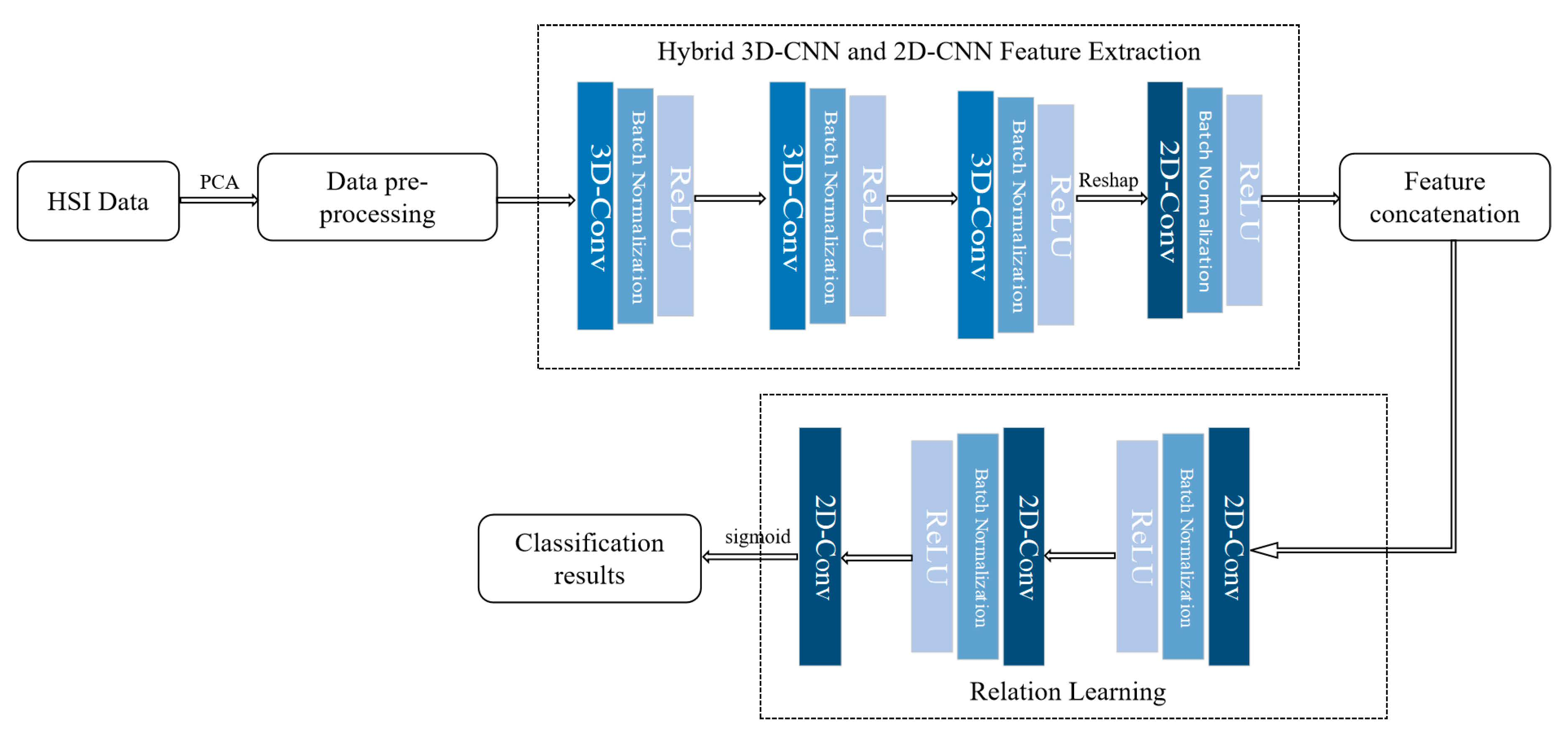
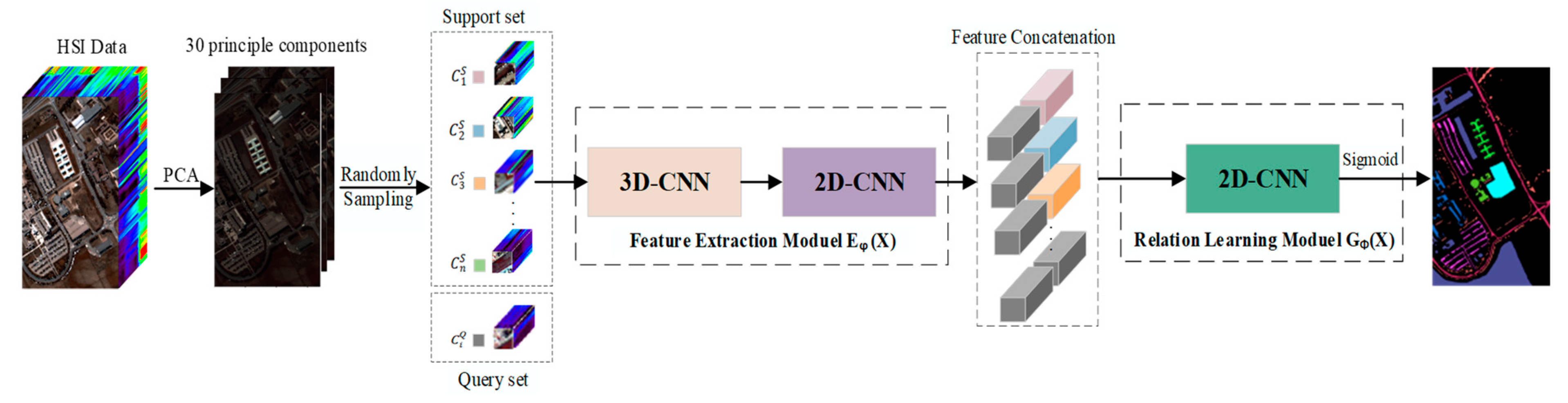
An H-RNet method is proposed for improved HSI classification that only requires a few labeled samples. In hybrid 3-D/2-D CNNs, spectral–spatial features are first obtained by 3D convolution, followed by further spatial information by 2D convolution, resulting in more discriminative features. In the relation learning module, sample pairing is used to efficiently obtain the relation scores under a small number of labeled samples for classification.
(2)
By innovatively combining the 3-D/2-D CNNs in a hybrid module with an end-to-end relation learning module, the H-RNet can more effectively extract the spatial and spectral features for improved classification of HSIs.
(3)
Experiments on three benchmark HSI datasets have demonstrated the superior performance of our approach over a few existing models.
This remaining article is organized as follows: Section 2 summarizes related work on CNNs and few-shot learning-based HSI classification. Section 3 details the proposed model. Section 4 presents the experimental results and analysis, followed by some concluding remarks in Section 5.

2. Related Work

2.1. HSI Classification Based on CNNs

CNNs have been extensively used in HSI classification in recent years; CNNs are more suitable for HSI processing and feature extraction [28,29]. Existing CNN models here include 1-D CNN, 2-D CNN and 3-D CNN, as detailed below. The 1-D CNN aims to extract deep features in the spectral domain [30], leading to a noise-sensitive performance due to the ignored spatial information. On the contrary, 2-D CNN extracts spatial information from the spectral-band-based images, where the spectral information is not emphasized. As a result, combining both 1D-CNN and 2D-CNN for extracting both spectral and spatial features is used for improved classification, such as in Zhang et al. [31] and Meng et al. [32]. To further explore the spatial information of HSI, Zheng et al. [33] proposed a rotation-invariant attention network (RIAN) for HSI classification, which is invariant to the spatial rotation of HSI. Although these methods attempt to make full use of both spectral and spatial features, they typically split the joint spectral–spatial features into two separate learning components, ignoring the correlation between spectral and spatial features.
As HSIs are essentially 3-D cubes, 3-D CNN-based classification has been naturally proposed to jointly extract the spectral–spatial information from HSIs. Chen et al. [34] were the first to use 3-D CNNs for HSI classification, but it suffers from high structural complexity and computational cost. Qing et al. [35] propose a 3D self-attention multiscale feature fusion network (3DSA-MFN) that integrates 3D multi-head self-attention. 3DSA-MFN first uses differently sized convolution kernels to extract multiscale features, samples the different granularities of the feature map, and effectively fuses the spatial and spectral features of the feature map. As a result, residual structures are proposed to solve these problems, such as an end-to-end spectral–spatial residual network (SSRN) in Zhong et al. [36] and a hierarchical residual network with an attention mechanism (HResnetAM) in Xue et al. [37]. In addition, Ghaderizadeh et al. [38] propose a multiscale dual-branch residual spectral–spatial network (MDBRSSN): the network extracts useful features through a two-branch structure.
Existing 2-D CNN and 3-D CNN models suffer from lack of information on the close correlation between the spectral and spatial information as well as network complexity. It is our aim to enhance feature representation capabilities to overcome the limitations of existing deep learning models and thus improve classification performance.

2.2. HSI Classification Based on Few-Shot Learning

Few-shot learning is a process where a model can effectively distinguish the categories in a new data set with only a very few labeled samples in processing the set [39,40]. To further reduce the reliance of the model on training samples, a number of few-shot learning methods have been proposed for HSI classification. Xi et al. [41] proposed a new FSL framework for the Class-Covariance Metric for HSIC (CMFSL); the CMFSL learns global class representations for each training episode by interactively using training samples from the base and novel classes. In Zhang et al. [42], a global prototype network (GPN) is proposed to map HSI data to an embedding space to learn the Euclidean distance between samples and complete the classification with a nearest neighbor classifier. In Liu et al. [43] a deep few-shot learning (DFSL) method is introduced using a 3-D CNN with residual blocks to learn the metric space and select the nearest neighbor (NN) or SVM classifier for classification. In Cao et al. [44], a 3-D Convolutional Siamese Network (3DCSN) is presented, which combines contrast information with label information for improved classification. In Alkhatib et al. [45], a Traditional CNN (Tri-CNN) approach to HSI classification was proposed, which is based on multi-scale 3D-CNN and three-branch feature fusion. However, all these methods use artificially set measurement distances, which may not be fully applicable to the features extracted by the neural network when classifying them. The relation network, in contrast, introduces a learnable metric function on the basis of the prototype network, where the relation module allows for a more accurate description of the differences between the samples. Deng et al. [46] designed a Similarity-Based Deep Metric Module (S-DMM), which effectively reduces the dependence of the model on samples and achieves improved HSI classification. Rao et al. [47] proposed a 3-D CNN-based spectral spatial relation network (SS-RN), which uses a relation network architecture to capture the deep correlation between samples accurately. Gao et al. [48] proposed a relation network model (RN-FSC) for few-shot HSI classification, which learns relationships between samples via a 3-D CNN and fine-tunes the model using a few labeled samples in the target dataset. Nevertheless, this method suffers from difficulties in training and a high computational cost.
Moreover, transfer learning is also an effective method to solve the problem of insufficient training samples [49]. Yang et al. [50] proposed a two-branch CNN (TWO-CNN) to learn the deep joint spectral–spatial features, and introduced a transfer learning strategy to improve the robustness of the proposed method. Liu et al. [51] combined data augmentation and transfer learning to address the lack of training data to further improve the HSI classification performance. Li et al. [52] proposed a transfer learning strategy for classifying HSIs. In the article, three different transfer methods for classifying HSIs were compared and analyzed. Zhang et al. [53] proposed a spectral-spatial self-attentive network (SSSAN) for HSI classification. Fang et al. [54] propose a 3D asymmetric inception network (AINet) to overcome the overfitting problem, The approach can use data-fusion transfer learning strategies to improve model initialization and classification performance.
Although the aforementioned methods have made great progress in HSI classification, the performance is severely degraded when only a limited number of labeled samples are available. This has led to a big challenge in deep learning models, as tackled in this article.

3. The Proposed Methodology

The problem of using only a few labeled samples to train deep learning models suffers from poor accuracy due to the imbalance between the huge parameter space and the small number of labeled samples. By increasing the amount of input training data through a sample pairing strategy, relation networks (RN) have been demonstrated to be an effective method for tackling training with limited training samples. The proposed hybrid relation network model (H-RNet) within a few-shot learning setting for HSI classification is detailed as follows.

3.1. Overall Structure

The overall flowchart of the proposed H-RNet for HSI classification is shown in Figure 1, which consists of three key modules, i.e., feature extraction, feature concatenation, and relation learning. Firstly, the principal component analysis (PCA) is applied to the HSI data for dimension reduction. Then, the data are randomly sampled and sent to the feature extraction module in order to obtain a feature map of the training: the pre-trained module. In the pre-processing section, the parameters are set to ensure that a fixed number of labeled samples can be taken at random for each class. This is achieved by randomly sorting the samples in each class, then selecting a fixed number of samples from each class and adding them to the training set in turn. Finally, the feature map of any two samples is combined to obtain the similarity scores of them through the relation learning module before being classified using the sigmoid function. A detailed summary of the proposed model in terms of the layer types, output map dimensions, and number of parameters is given in Table 1.

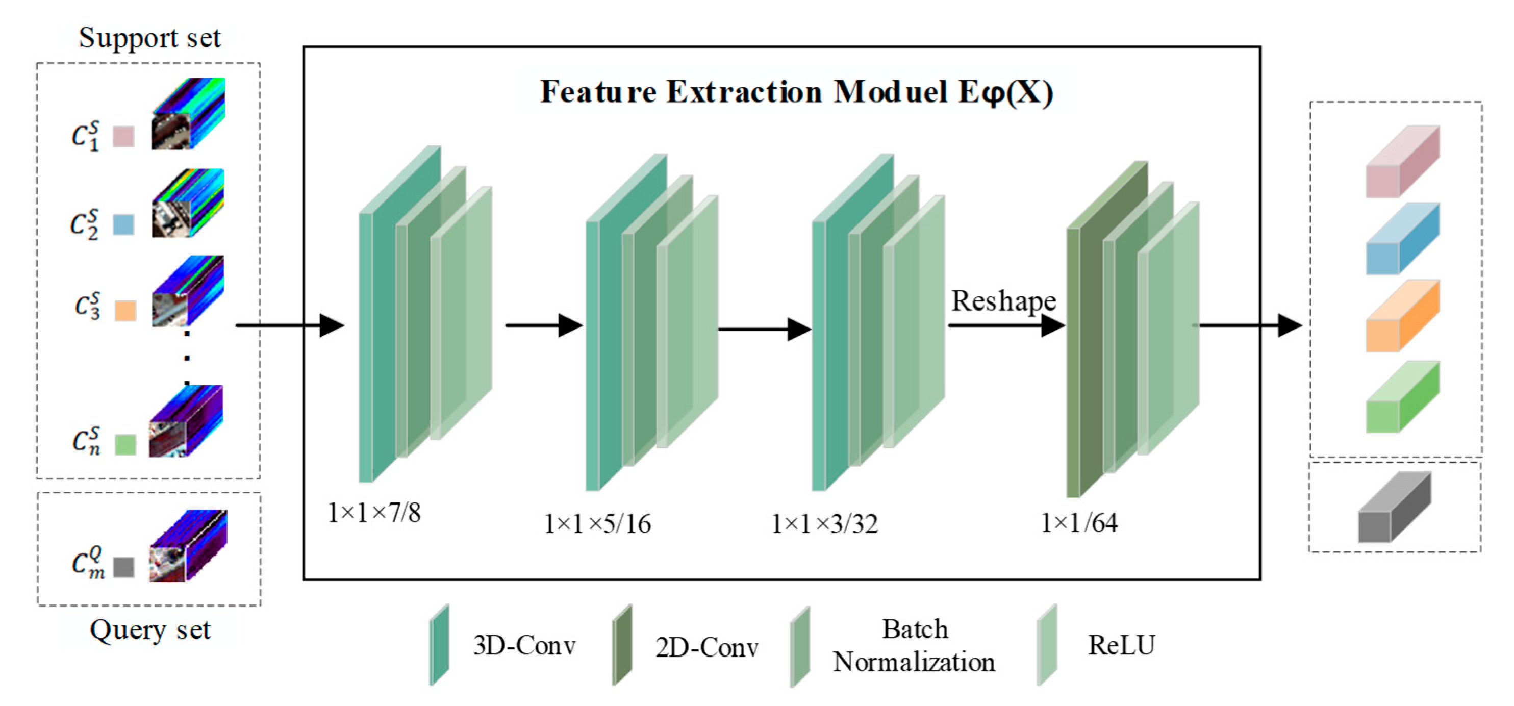
3.2. Hybrid 3D-CNN and 2D-CNN Feature Extraction Module

H-RNet aims to extract more discriminative features from the input data. Inspired by the literature of [55], we use a hybrid 3D-2D CNN module for feature extraction, which will obtain more effective spectral–spatial feature extraction for HSI classification while reducing the complexity of the model. The spectral–spatial features are first obtained by 3D convolution, followed by further spatial information by 2D convolution, resulting in more discriminative features and lower network complexity compared to 3D convolutional neural networks. As shown in Figure 2, the proposed feature extraction module consists mainly of three 3-D CNN blocks and one 2-D CNN block. Each block consists of a convolutional layer, a batch normalisation layer (BN), and a Relu activation function. Adding a BN after each convolutional layer mitigates the gradient disappearance problem and enhances the generalization ability. The Relu activation function is widely used in deep learning to improve the non-linearity of the model and speed up the convergence rate. The overall convolution kernel is chosen to be 1 × 1 in size to significantly reduce the number of parameters and facilitate training with only a few samples.
After completing feature extraction, the next step is feature concatenation. In this process, the training set is first divided into support set and query set. Specifically, one labeled sample is randomly selected from each class as the support set, and half of the total samples from each class are randomly selected as the query set (samples in the query set are different from those in the support set). The feature concatenation operation involves pairing each query sample with each support sample to form sample pairs, which are then input into the relation network to complete the classification task.
Convolution is implemented as follows: The training samples are fed into the 3-D convolutional network, and 3-D convolutional operations are applied to the spatial-spectral domain to obtain the correlation between multiple spectral bands. When calculating the 3-D convolution, the activation value at the (x, y, z) position on the jth feature map at layer i is given by
v i , j x , y , z = f μ w = 0 W i 1 l = 0 L i 1 d = 0 D i 1 θ i , j , μ w , l , d v i 1 , μ x + w , y + l , z + d + b i , j
where f () and b i , j denote the non-linear activation function and the bias, respectively. W i , L i , and D i are the width, height, and spectral dimension of the 3-D convolution kernel, respectively. θ i , j , μ w , l , d denotes the weight parameter at the jth feature map location ( l , w , d ) in layer i. v i 1 , μ x + w , y + l , z + d denotes the value at ( x + w , y + l , z + d ) in the th feature map of the previous layer.
For 2-D convolution, it further learns more abstract spatial features from the outcomes of the 3-D convolutions, resulting in more discriminative spectral–spatial features. In the 2D-CNN, the spatial dimension of the feature map is convolved using a 2-D convolution kernel, and the results in different channels are then summed with pixels to obtain a 3-D tensor. The jth feature map v i , j x , y at ( x , y ) of the ith layer is given by
v i , j x , y = f μ w = 0 W i 1 l = 0 L i 1 θ i , j w , l v i 1 , μ x + w , y + l + b i , j

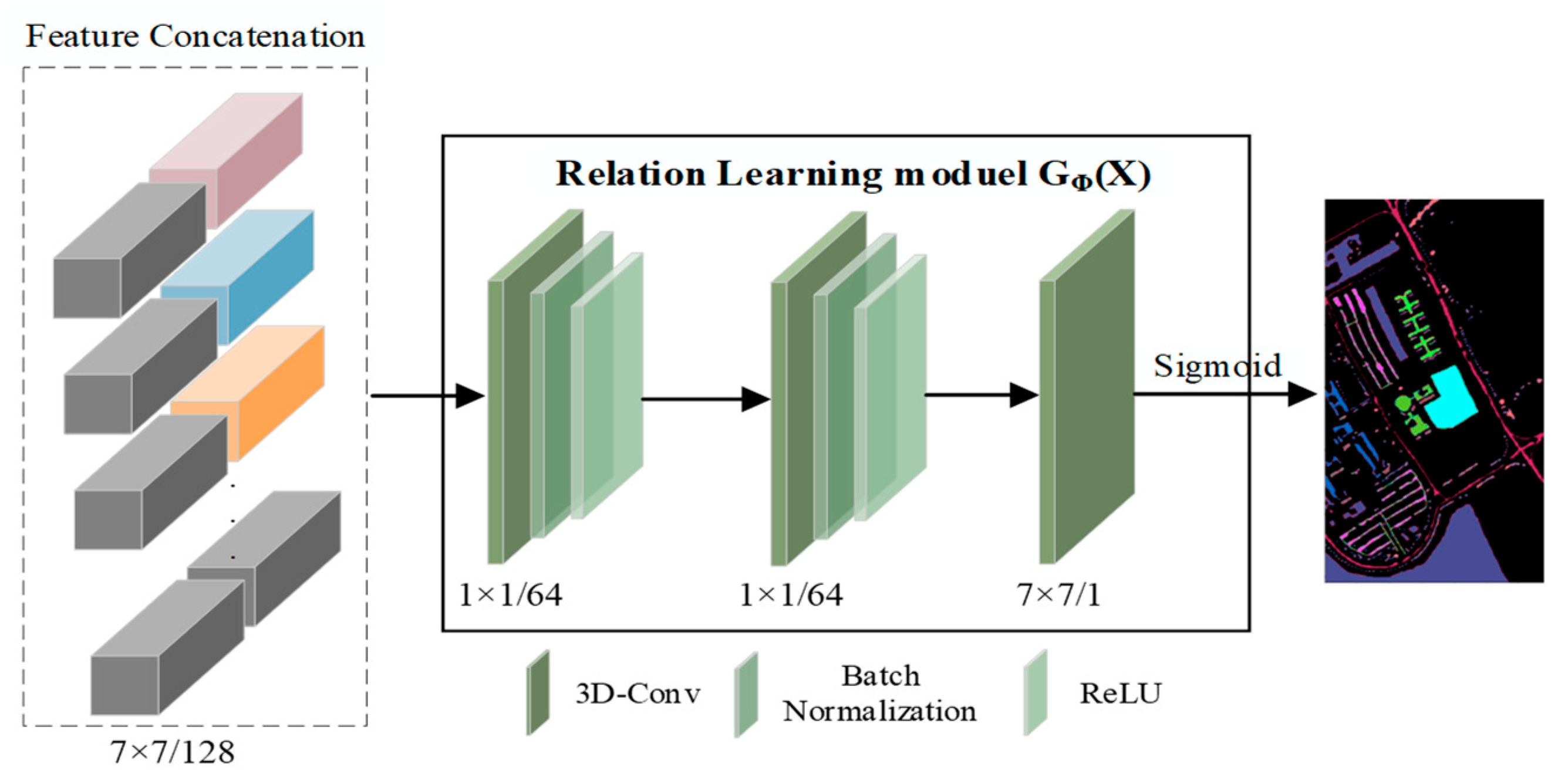
3.3. Relation Learning Module

The relation learning module is one of the core components of the relation network and is mainly used to learn the similarity between different samples and to perform classification. The purpose of the relation learning module is to obtain the similarity between any pair of training samples. In the relation learning module, the feature map obtained from the feature concatenation operation is fed into the neural network, and the relation score between different samples is calculated by comparing their similarities. Samples within the same category are assigned higher relation scores, while samples between different categories are assigned lower relation scores. In this way, the relation learning module can better capture the relation information between samples, thereby improving the classification accuracy and robustness of the model. The relational learning module is shown in Figure 3:
As can be seen in Figure 3, the relation learning module of H-RNet is centered on three two-dimensional CNN blocks. The feature extraction module obtains two features concatenated together as a 128 × 7 × 7 tensor (7 × 7 is the neighbor window size). The tensor is then fed into a two layer 2-D CNN, which uses a 1 × 1 convolution kernel to effectively reduce the dimensionality while extracting features, considering that the number of channels is much larger than the spatial dimensionality. To thoroughly train the network, a BN layer and a Relu activation function are also applied after each convolution. It then enters a 7 × 7 2-D convolution layer that converts the feature map into a relation score. Finally, a sigmoid function is used to generate the output to describe the similarity between samples at a specified scale, with the function taking values in the range [0, 1]. The relation learning module can be expressed as the following equation:
r i , j = G ϕ ( C ( E φ ( x i ) , E φ ( x j ) ) )
where the symbol C() is the operator for deep stitching, E φ ( ) is the deep feature map obtained by the feature extraction module, and G ϕ ( ) is the function to obtain the relation score.
H-RNet is trained on the model using the mean square error (MSE), which is simple to calculate and train, and the loss function is given by
φ , ϕ argmin φ , ϕ i = 1 C × K j = 1 C × N ( r i , j 1 · y i = = y j )
By optimizing Equation (4), the model can learn to measure the similarity between two samples and compare whether they belong to the same class.
In this article, training is performed using an episode-based strategy. To be specific, the classification task is denoted as a C-way K-shot N-query task, where C denotes the total number of classes in each task, K denotes the number of training samples per class, and N denotes the number of query samples per class. Our experiments are conducted in a few-shot setting with 10 labeled samples per class. In each iteration, the C classes are randomly selected from the training samples, and K labeled samples from each class are used as input to the support set. The support set is represented as S = x i , y i i = 1 C × K . Meanwhile, we randomly select N samples from each of the same C categories as the support set as the query set, and the query set is denoted as Q = x j , y j j = 1 C × N . The query set has no intersection with the support set. The H-RNet model training process is given in Algorithm 1.
Algorithm 1 H-RNet model training process
Input: Support set S = x i , y i i = 1 C × K and Query set Q = x j , y j j = 1 C × N for each iteration. Initializing feature extraction module E φ and relation learning module G ϕ .
Output: Update the parameters of module ( E φ ,   G ϕ ) .
1.   for (x′, y′) in Q do
2:         for (x, y) in S do
3:               The feature extraction module obtains the features E φ ( x ) and E φ ( x ) from x and x′;
4:               Update the relation score by Equation (3);
5:               pdate the loss by Equation (4);
6:          end for
7:       end for
8: Update the parameters of E φ and G φ by L back propagation.
9: Repeat iterations until the completion of the training process.

4. Experiment and Discussion

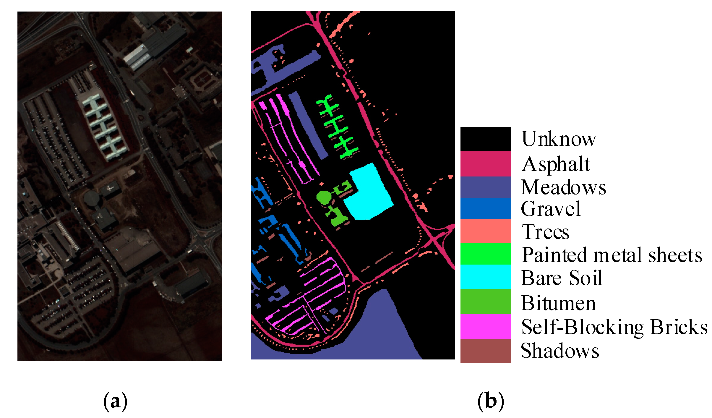
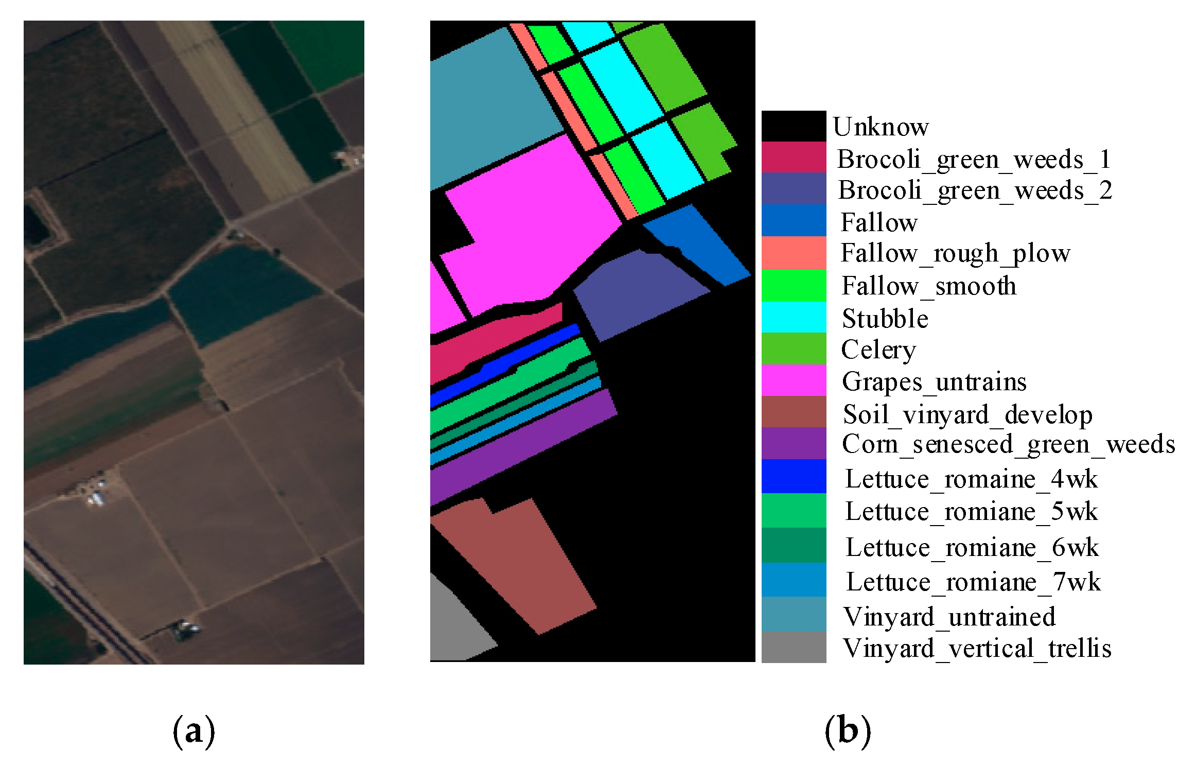
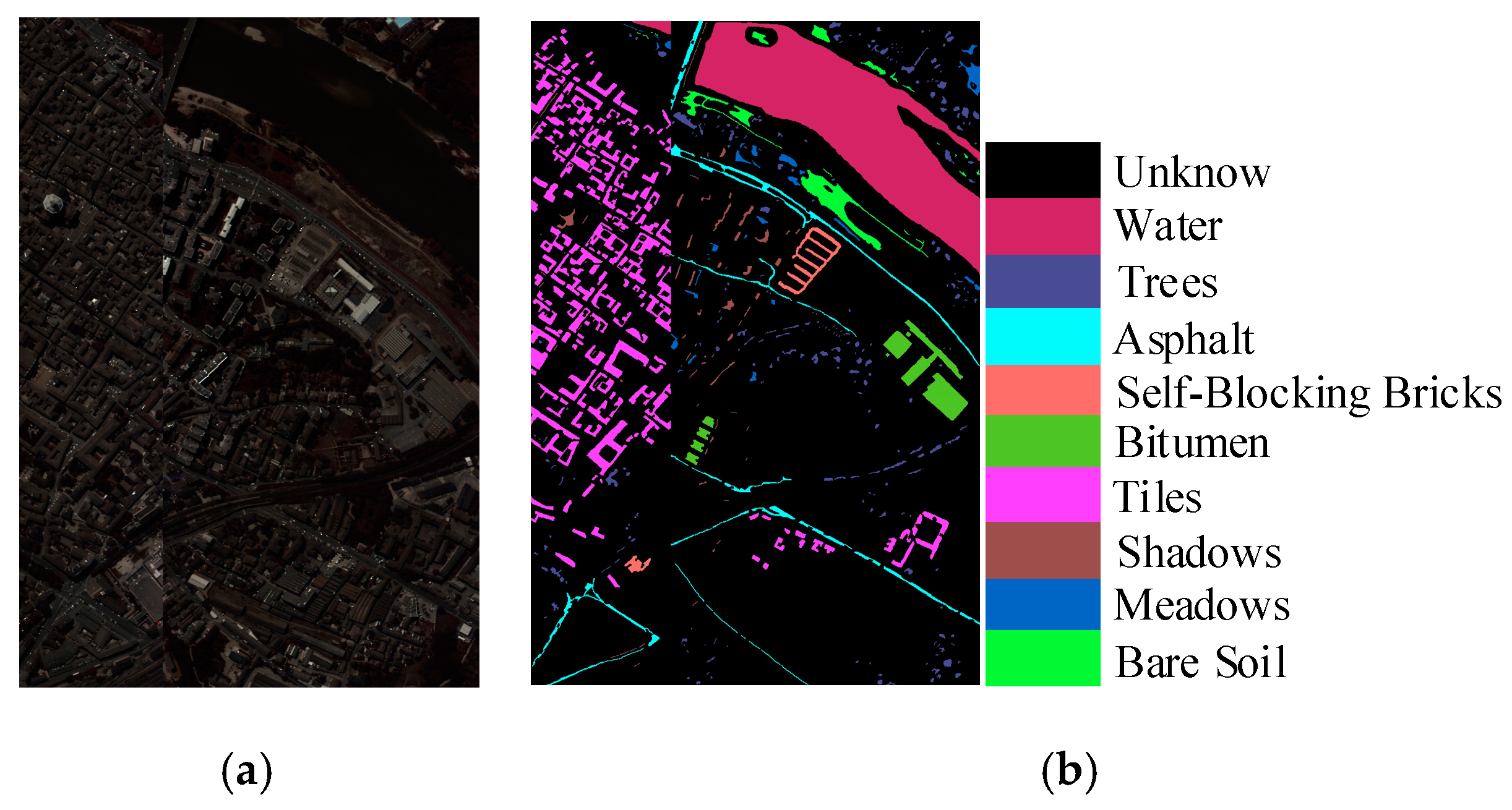
4.1. Dataset Description

For performance assessment, three publicly available datasets, namely the Pavia University dataset, the Salinas dataset, and the Pavia Centre dataset, are used, as detailed below.
Pavia University (PU) dataset: This dataset was collected by the ROSIS sensor in Italy’s University of Pavia campus. It consists of 610 × 340 pixels covering nine types of ground truth samples. Specifically, excluding the 12 bands affected by noise, it contains 103 spectral bands with a wavelength range of 430–860 nm and a spatial resolution of 1.3 m. Figure 4 shows the false-color image and the labeled image of the PU dataset.
Salinas (SA) dataset: acquired by the AVIRIS imaging spectrometer in the region over the Salinas Valley, California, and the image consists of 512 × 217 pixels. Concretely, the 20 bands affected by noise are removed, leaving 204 spectral bands, and the resulting image has a spatial resolution of 3.7 m. These data are non-urban area data and contain 16 classes of features. Figure 5 shows the false-color image and the labeled image of the SA dataset.
Pavia Centre (PA) dataset: also taken by the ROSIS sensor and contains nine classes with an image size of 1096 × 715 pixels. In particular, excluding the 13 bands affected by noise, it includes 102 spectral bands, and the resulting image has a spatial resolution of 1.3 m. Figure 6 shows the false-color image and the labeled image of the PA dataset.

4.2. Experimental Settings

The proposed method is implemented using the PyTorch framework in the python language. All experiments were conducted on a desktop computer with an NVIDIA GeForce GTX 1080 graphics processor (GPU) with 16 GB RAM. An Adam iterator was used for training on the three datasets with an initial learning rate of 0.001. To ensure convergence, the training iterations were 1000, and after half the number of iterations, the learning rate was divided by 10. A C-way K-shot N-Query episode represented each iteration. For the PU and PA datasets, C was set to 9, and on the SA dataset, it was set to 16. K and N are set to 1 and 5, respectively, based on experience from previous studies.
For consistency, we use the overall accuracy (OA), the average accuracy (AA), and the kappa coefficient (κ) to quantitatively assess the classification performance of different methods [56,57]. OA is used to measure the accuracy of all classification results, i.e., the ratio of correctly classified samples to the total number of samples. AA is the average classification accuracy for each class, reflecting the model’s adaptability to different classes. The kappa coefficient measures the overall classification results and better reflects the classification performance on unbalanced data sets, with values usually ranging from 0 to 1. In addition, to comprehensively evaluate the accuracy of the experiment, we also analyzed the F1-score. F1-score is a comprehensive evaluation index of the model, which takes into account both precision and recall, and is an important indicator for evaluating the performance of classifiers.

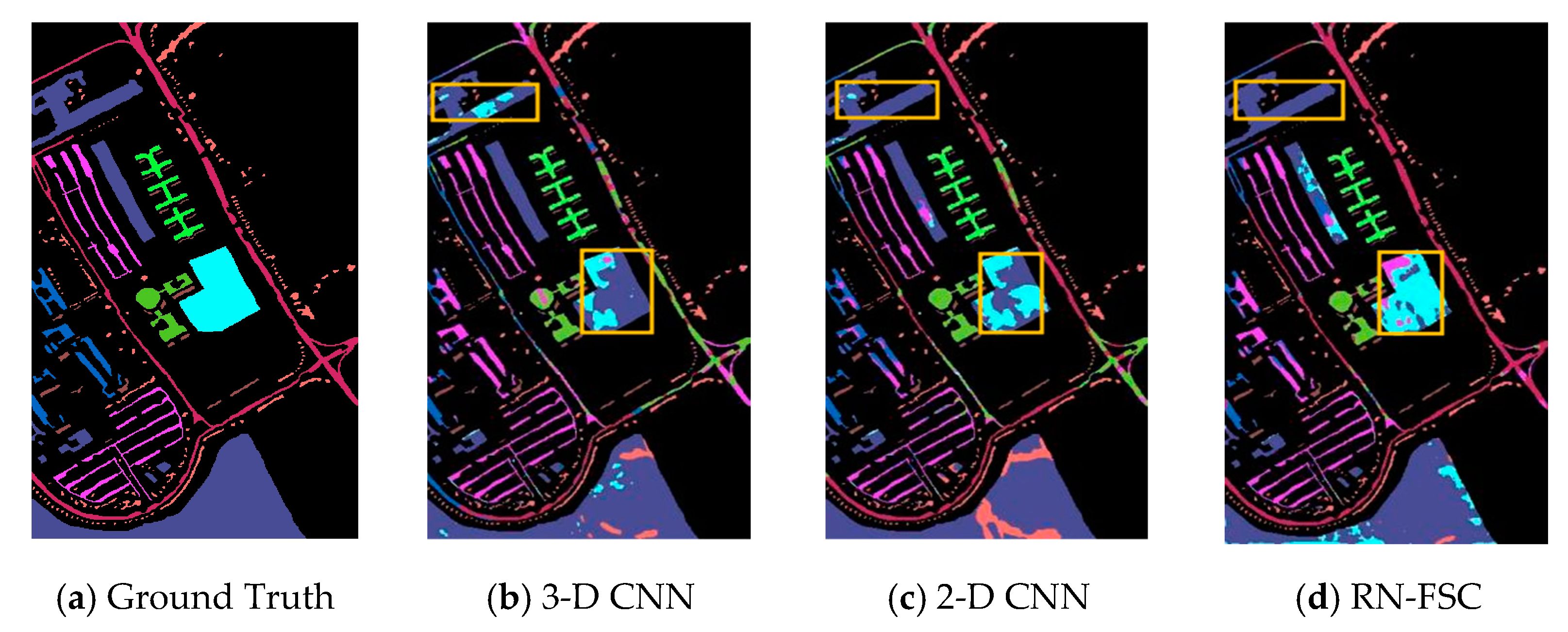
4.3. Classification Results

For performance evaluation, the proposed method is compared with a few mainstream supervised deep learning and few-shot learning methods. The former include 2-D CNN models [18], 3-D CNN models [20], hierarchical residual models with attention mechanisms (HResNetAM) [37], and two-stream convolutional networks based on transfer learning (TWO-CNN) [50]. The latter include 2-D CNN-based relation networks (S-DMM) [46], metric-based learning classification (DFSL-NN) [43], 3-D Siamese network- based 3DCSN [44], and 3D-CNN-based relation network (RN-FSC) [48] models. Again, 10 labeled samples per class were randomly selected for training the models. Table 2, Table 3 and Table 4 showed the mean and standard deviation (std) of the classification accuracy obtained in 10 runs on the PU, SA, and PA datasets, respectively.
Table 2 shows the classification results of different methods on the PU dataset, where our algorithm achieved the highest classification accuracy on all three evaluation metrics. Compared to the state-of-the-art few-shot learning methods DFSL-NN, S-DMM, 3DCSN, and RN-FSC, our approach surpassed them by 3.81%, 4.12%, 3.45%, and 5.88% in OA, by 5.07%, 2.24%, 5.66%, and 10.67% in AA, and by 5.24%, 1.62%, 3.06%, and 9.26% in the kappa, respectively, as well as exceeding by 0.025, 0.06, and 0.006 in terms of F1-score. This is mainly because the hand-crafted distance functions in both DFSL-NN and the 3DCSN may be unsuitable for the extracted features for classification. In addition, the 2-D CNN-based S-DMM has limitations in only extracting spatial information but ignoring the spectral one. The RN-FSC framework is a 3-D relation network, yet it fails to extract more effective spectral–spatial features than our approach and has a much more complicated architecture than our hybrid 3-D/2-D networks.
Generally, with only 10 samples per class, the few-shot learning algorithms achieve better results than other supervised deep learning methods. It is worth noting that the HResNetAM method has also produced quite good results due mainly to the multi-scale spectral–spatial information extracted from its hierarchical residual structure. Here the 2-D CNN model outperformed the 3-D CNN, due to the data augmentation adopted. Overall, the results above have fully demonstrated the effectiveness of our approach in classifying the HSI in the few-shot learning setting.
Table 3. Classification results of different methods on the SA dataset with 10 samples per class for training.
Class2D-CNNTWO-CNN3D-CNNDFSL-NNS-DMM3DCSNRN-FSCHResNetAMH-RNet
(Ours)
198.8088.2296.9998.5499.45100.096.3599.6799.89
298.7778.0999.2598.1299.2198.97100.099.6099.76
395.4874.8092.6096.0896.7099.49100.096.7699.99
498.3698.1997.2199.5699.56100.086.8895.3799.37
592.5596.5492.9997.0197.1291.0799.8899.7998.42
699.9696.8998.5499.5489.6498.55100.099.9399.88
799.6192.5297.6599.3399.8299.49100.098.9299.92
877.5154.3270.2178.6270.5370.7489.4486.7181.48
997.1981.2295.0097.2399.0299.9099.9398.8499.97
1089.2375.1884.5492.3891.1396.5199.1993.4195.12
1195.4592.2692.8399.1097.56100.097.3494.2199.61
1299.9686.4098.0999.3499.8789.7790.6199.2699.75
1399.2298.1895.6297.8499.2599.0184.0999.4599.67
1496.8096.1093.5096.1796.3098.1188.5795.2099.03
1572.0355.6065.3772.6972.2894.1170.0671.2085.61
1694.0792.3993.6198.5995.2993.8789.9899.9498.14
OA (%)91.31
±0.53
77.54
±2.15
85.93
±1.48
89.86
±0.84
89.69
±2.98
91.59
±1.39
91.45
±1.72
91.56
±0.84
93.67
±0.72
AA (%)94.06
±0.39
84.94
±1.72
90.56
±1.02
95.01
±0.63
93.92
±0.92
95.60
±0.85
93.27
±1.04
95.54
±0.66
97.23
±0.26
κ × 10090.12
±0.20
76.17
±2.69
82.68
±0.25
89.51
±0.31
88.69
±3.26
90.68
±0.94
90.52
±0.74
90.62
±0.23
92.96
±0.79
F1-score0.951
±0.064
-0.901
±0.062
-0.937
±0.034
0.946
±0.017
0.910
±0.040
0.954
±0.021
0.963
±0.057
Table 3 compares the classification results on the SA dataset, where the similar observations and conclusions can be found to further validate the efficacy of our proposed approach. Among the top-five highly performed approaches, our method significantly outperformed the other four. The improvements are 3.81%, 3.98%, 2.08%, and 5.88% in OA, 2.22%, 3.31%, 2.28%, and 3.31% in AA, and 3.45%, 4.27%, 2.28%, and 6.72% in Kappa, respectively. For the F1-score, our method improved over S-DMM, 3DCSN, and RN-FSC by 0.026, 0.017, and 0.012, respectively. The analysis of this parameter gives a fuller picture of the effectiveness of our proposed method.
Table 4. Classification results of different methods on the PA dataset with 10 samples per class for training.
ClassTWO-CNN3D-CNNDFSL-NNS-DMM3DCSNHResNetAMH-RNet
(Ours)
198.7298.9797.2899.9596.4299.9899.87
295.8297.8895.4694.5692.6498.5192.19
380.2984.5885.4688.3184.5781.0295.71
461.9562.5984.6992.6799.4773.8596.32
595.6794.8694.1095.2298.5396.2693.39
690.5892.4793.4692.0391.1489.7299.02
793.2091.3896.6197.5097.8498.5490.73
898.2795.4599.9899.8499.5699.8999.37
997.7586.9796.0798.1684.0896.4299.81
OA (%)95.47
±1.06
95.07
±0.38
97.79
±0.51
96.98
±1.21
96.54
±1.78
97.74
±0.63
98.23
±0.45
AA (%)90.25
±1.79
89.32
±2.24
93.68
±0.87
95.36
±0.94
93.81
±1.28
92.69
±0.47
96.28
±1.36
κ × 10093.69
±0.97
92.45
±1.94
97.02
±0.14
96.25
±0.81
95.14
±1.02
96.81
±0.89
97.49
±0.63
F1-score---0.900
±0.018
0.926
±0.054
0.904
±0.053
0.944
±0.049
Table 4 shows the classification results on the PA dataset; again, our approach has produced the best results with an OA of 98.40%. Compared to other few-shot learning methods of DFSL-NN, S-DMM, and 3DCSN, the improvements are 0.44%, 1.25%, and 1.69% in OA, 2.60%, 0.92%, and 2.47% in AA, and 0.47%, 1.24%, and 2.35% in the Kappa, respectively. For the F1-score, our method improved over S-DMM, 3DCSN, and RN-FSC by 0.044, 0.018, and 0.040, respectively. For classes that cannot be accurately classified by other methods, such as Asphalt and Bare Soil, our approach can still produce very accurate classification results. This has further demonstrated the effectiveness of our proposed model in classifying HSIs even within a quite small number of labeled samples.
In Figure 7, Figure 8 and Figure 9, the classification maps from different approaches for the three datasets are given for visual comparison. As seen in Figure 7, of all the classification maps for the PU dataset, some pixels in the purple ‘Grass’ and blue ‘Bare Soil’ boxes in the yellow box are easily misclassified because these two land cover areas have very similar spectral spatial characteristics. It can be observed that our method has reduced misclassification on these two features compared to the other methods. Overall, the classification map obtained by our H-RNet seem to be the smoothest and most accurate in comparison to the ground truth. Similar and consistent observations can be also found in Figure 8 and Figure 9, which have further demonstrated the efficacy of the proposed approach.

4.4. Ablation Study

4.4.1. Impact of the Number of Principal Components

The number of principal components (PC) has a significant impact on the performance of our H-RNet model in terms of accuracy and efficiency. Experiments were conducted on three datasets with different PC values, where PC values were chosen as 20, 30, 40, and 50, the results of which are shown in Table 5.
As seen in Table 5, the best classification accuracy is achieved when the PC value is 30 on both the PU and SA datasets. For the PA dataset, there is not much difference in the classification results for different PC values. Therefore, we set the PC value to 30 in our experiments for simplicity.

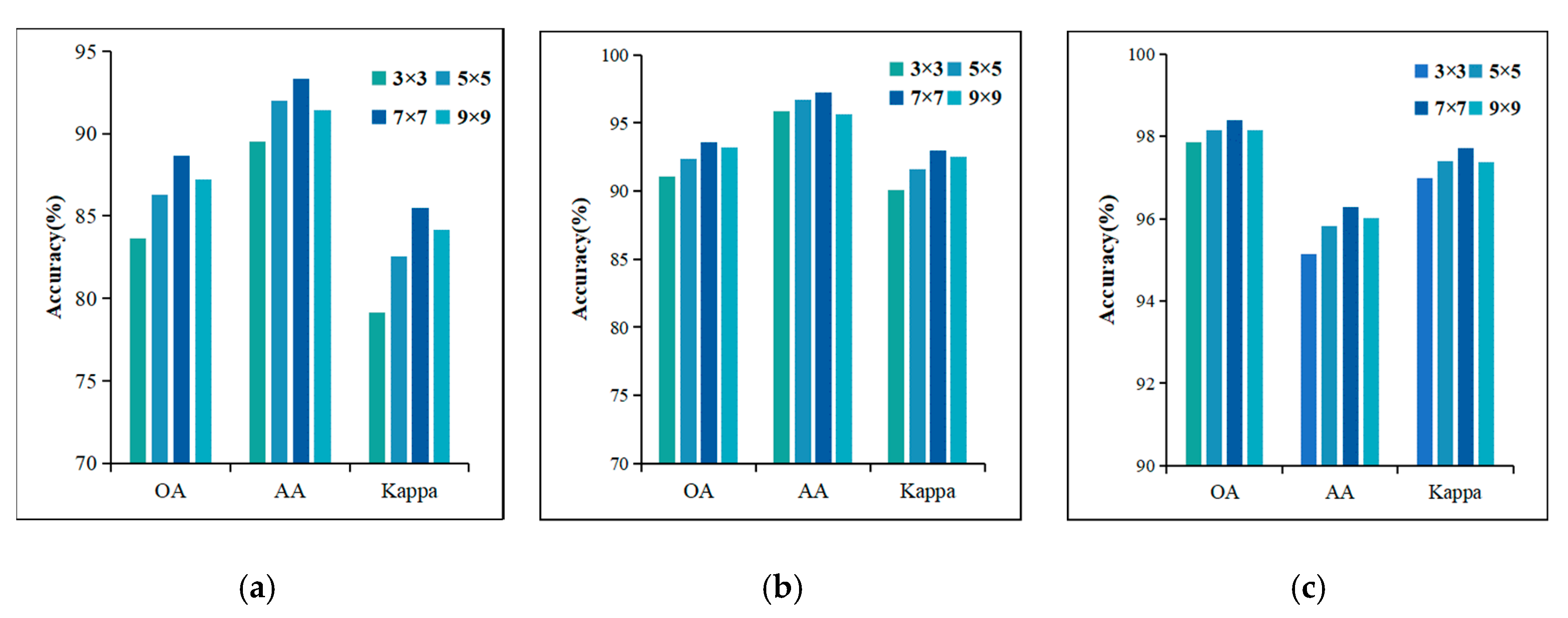
4.4.2. Impact of the Patch Size

As we take the entire neighbor of a pixel as input, the neighbor window size P × P will affect the classification performance; its effect is shown in Figure 7 when varying the window size from 3 × 3 to 9 × 9.
As seen in Figure 10, when the patch size increases from 3 × 3 to 7 × 7, the accuracy gradually increases, due to the fact that larger samples may contain more spatial information. However, when the patch size reaches 9 × 9, the accuracy of all three datasets starts to decrease, due possibly to the increasing number of interfering pixels degrading the classification performance. Therefore, we set the patch size as 7 × 7 in this article.

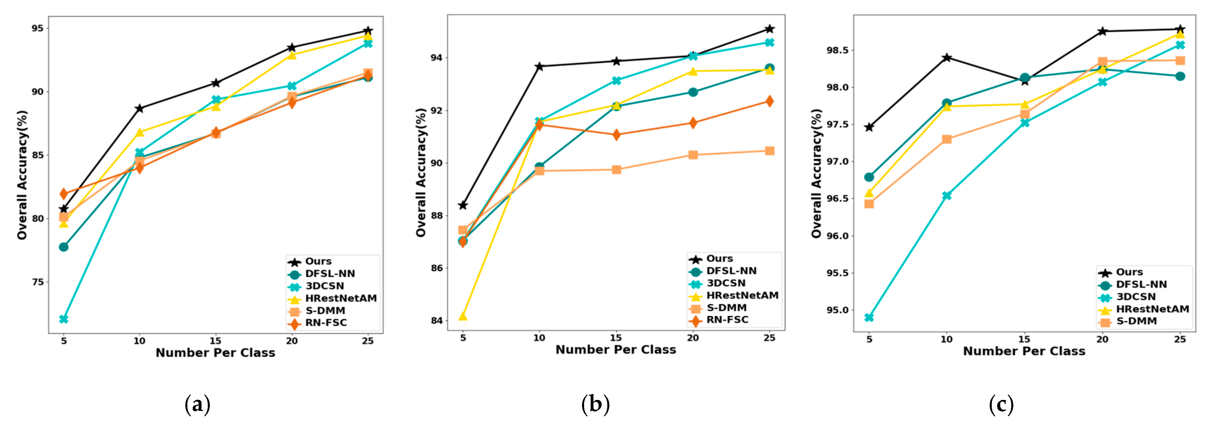
4.4.3. Impact of the Number of Labeled Samples per Class

To further validate the advantages of the H-RNet in the few-shot learning setting, a comparison was performed with different numbers of labeled samples per class. For each class, 5, 10, 15, 20, and 25 labeled samples were randomly selected for training the models with the results compared in Figure 11.
As seen in Figure 11, the classification results gradually improve with the increasing number of training samples on all three datasets. Our method consistently achieves better classification accuracy on all three datasets. On the PA dataset, when the number of training samples per class is five, the classification accuracy of our method is only lower than that of RN-FSC. On the PA dataset, ours is comparable to that of DFSL-NN when the number of training samples per class is 15. This advantage is even more apparent when there are only 10 labeled samples per class. Therefore, to make the contrast more obvious, we set the number of training samples per class to 10.

4.5. Computational Complexity Analysis

In this section, the number of model parameters and FLOPs for different methods are given in Table 6, which mainly include two types of deep network methods based on supervised learning and few-shot learning. The deep learning methods based on supervised learning include 2D-CNN, TWO-CNN, and HResNetAM, and the methods based on few-shot learning include DFSL-NN, 3DCSN, S-DMM, and RN-FSC. Compared with the three methods in the first category, our method simply has a higher number of parameters than 2D-CNN; this is because 2D-CNN only utilizes spatial information and has a simpler model, while our method uses 3D-CNN to obtain spectral–space information, and thus the number of our parameters will be higher. In comparison to HResNetAM and TWO-CNN, HResNetAM is a 3D-CNN residual-based network while TWO-CNN is a two-branch-based network structure, both of which can obtain both spectral and spatial information. Our approach has lower network complexity and achieves higher classification results than both networks.
Compared to the four few-shot learning methods, DFSL-NN is a metric-based method, 3DCSN is a Siamese network-based method, and S-DMM and RN-FSC are based on 2D and 3D relation networks respectively. Our method has the highest classification accuracy compared to these methods, but its parameter count is higher than S-DMM because S-DMM has a simpler model structure based on 2D-CNN. However, compared to the RN-FSC method based on 3D relation networks, our method has fewer network parameters due to the combination of 3D/2D convolutions, which can extract more discriminative features and therefore be more advantageous for classification. In summary, through parameter analysis, we have verified that our method has lower network complexity and can achieve higher classification accuracy.
Table 6. Comparison of model parameters on the PU dataset.
ModelFLOPs (M)Params (M)
2D-CNN1.7735,536
TWO-CNN239.021,574,506
HResNetAM803.05343,587
DFSL-NN416.4856,848
3DCSN1967.951,537,256
S-DMM82.2928,929
RN-FSC816.44402,465
H-RNet (Ours)72.9855,845

5. Conclusions

In this article, we propose a new deep learning network, H-RNet, based on few-shot learning for effective feature extraction and data classification in HSIs. Firstly, our method can better extract spatial and spectral information from high-dimensional data while maintaining a relatively simple model structure and fewer parameters by using a mixed 3D/2D CNN, even with limited labeled samples. Secondly, experiments were conducted on three public datasets, and our method was compared with several other methods. The experimental results demonstrate that the H-RNet method has higher accuracy and robustness in high-dimensional image classification tasks than other methods. Finally, because the transfer learning method proposed in this article is limited to the same domain, future research will also consider the study of few-shot learning-based transfer learning for HSI classification across different datasets.

Author Contributions

Conceptualization, Z.D.; methodology, Z.D.; validation, X.L., J.R. and H.L. (Huihui Li); formal analysis, H.L (Huihui Li). and Z.D.; investigation, Z.D.; resources, H.Z.; data curation, W.C., Z.X. and H.L. (Hao Li); writing—original draft preparation, Z.D.; writing—review and editing, X.L., J.R. and H.L. (Huihui Li); visualization, Z.D. and J.R.; supervision, H.Z., W.C. and Z.X.; project administration, X.L. and H.L. (Huihui Li); funding acquisition, X.L. and H.L. (Huihui Li). All authors have read and agreed to the published version of the manuscript.

Funding

This study was supported by National Natural Science Foundation of China (Grant Nos. 62172113, 62006049, and 61906216), The Ministry of Education of Humanities and Social Science project (Grant No. 18JDGC012), Guangdong Provincial Key Laboratory Project of Intellectual Property and Big Data (Grant No. 2018B030322016), Guangdong Science and Technology Project (Grant Nos. KTP20210197 and 2017A040403068), Project of Education Department of Guangdong Province (Grant No. 2022KTSCX068), Project of Guangdong Polytechnic Normal Universityon (Grant No. 22GPNUZDJS16), and Guangdong Basic and Applied Basic Research Foundation (Grant No. 2023A1515010939).

Data Availability Statement

All three hyperspectral image datasets used are available online at https://www.ehu.eus/ccwintco/index.php?title=Hyperspectral_Remote_Sensing_Scenes# (accessed on 1 December 2021).

Conflicts of Interest

The authors declare no conflict of interest.

References

  1. Kumar, B.; Dikshit, O.; Gupta, A.; Singh, M.K. Feature Extraction for Hyperspectral Image Classification: A Review. Int. J. Remote Sens. 2020, 41, 6248–6287. [Google Scholar] [CrossRef]
  2. Huang, K.; Deng, X.; Geng, J.; Jiang, W. Self-Attention and Mutual-Attention for Few-Shot Hyperspectral Image Classification. In Proceedings of the 2021 IEEE International Geoscience and Remote Sensing Symposium IGARSS, Brussels, Belgium, 11–16 July 2021; pp. 2230–2233. [Google Scholar] [CrossRef]
  3. Yalamarthi, S.; Joga, L.K.; Madem, S.R.; Vaddi, R. Deep Net based Framework for Hyperspectral Image Classification. In Proceedings of the 2022 7th International Conference on Communication and Electronics Systems (ICCES), Coimbatore, India, 22–24 June 2022; pp. 1475–1479. [Google Scholar] [CrossRef]
  4. Yuan, Y.; Wang, C.; Jiang, Z. Proxy-Based Deep Learning Framework for Spectral–Spatial Hyperspectral Image Classification: Efficient and Robust. IEEE Trans. Geosci. Remote Sens. 2022, 60, 5501115. [Google Scholar] [CrossRef]
  5. Chen, R.; Huang, H.; Yu, Y.; Ren, J.; Wang, P.; Zhao, H.; Lu, X. Rapid Detection of Multi-QR Codes Based on Multistage Stepwise Discrimination and A Compressed MobileNet. IEEE Internet Things J. 2023; early access. [Google Scholar] [CrossRef]
  6. Zheng, X.; Chen, W.; Lu, X. Spectral Super-Resolution of Multispectral Images Using Spatial-Spectral Residual Attention Network. IEEE Trans. Geosci. Remote Sens. 2022, 60, 5404114. [Google Scholar] [CrossRef]
  7. Li, Y.; Ren, J.; Yan, Y.; Petrovski, A. CBANet: An End-to-end Cross Band 2-D Attention Network for Hyperspectral Change Detection in Remote Sensing. IEEE Trans. Geosci. Remote Sens. 2023, in press. [Google Scholar]
  8. Zhao, J.; Hu, L.; Dong, Y. A combination method of stacked autoencoder and 3D deep residual network for hyperspectral image classification. Int. J. Appl. Earth Obs. Geoinf. 2021, 102, 102459. [Google Scholar] [CrossRef]
  9. Zhao, C.; Li, C.; Feng, S.; Li, W. Spectral-Spatial Anomaly Detection via Collaborative Representation Constraint Stacked Autoencoders for Hyperspectral Images. IEEE Geosci. Remote Sens. Lett. 2022, 19, 5503105. [Google Scholar] [CrossRef]
  10. Zabalza, J.; Ren, J.; Zheng, J. Novel segmented stacked autoencoder for effective dimensionality reduction and feature extraction in hyperspectral imaging. Neurocomputing 2016, 185, 1–10. [Google Scholar] [CrossRef]
  11. Hang, R.; Liu, Q.; Hong, D.; Ghamisi, P. Cascaded Recurrent Neural Networks for Hyperspectral Image Classification. IEEE Trans. Geosci. Remote Sens. 2019, 57, 5384–5394. [Google Scholar] [CrossRef]
  12. Li, H.C.; Li, S.S.; Hu, W.S.; Feng, J.H.; Sun, W.W.; Du, Q. Recurrent Feedback Convolutional Neural Network for Hyperspectral Image Classification. IEEE Geosci. Remote Sens. Lett. 2022, 19, 5504405. [Google Scholar] [CrossRef]
  13. Mughees, A.; Tao, L. Multiple Deep-Belief-Network-Based Spectral-Spatial Classification of Hyperspectral Images. Tsinghua Sci. Technol. 2019, 24, 183–194. [Google Scholar] [CrossRef]
  14. Shi, C.; Liao, D.; Zhang, T.; Wang, L. Hyperspectral Image Classification Based on Expansion Convolution Network. IEEE Trans. Geosci. Remote Sens. 2022, 60, 5528316. [Google Scholar] [CrossRef]
  15. Wang, X.; Tan, K.; Du, P.; Pan, C.; Ding, J. A Unified Multiscale Learning Framework for Hyperspectral Image Classification. IEEE Trans. Geosci. Remote Sens. 2022, 60, 4508319. [Google Scholar] [CrossRef]
  16. Li, C.; Fan, T.; Chen, Z.; Gao, H. Directionally separable dilated CNN with hierarchical attention feature fusion for hyperspectral image classification. Int. J. Remote Sens. 2022, 43, 812–840. [Google Scholar] [CrossRef]
  17. Imani, M.; Ghassemian, H. An overview on spectral and spatial information fusion for hyperspectral image classification: Current trends and challenges. Inf. Fusion 2020, 59, 59–83. [Google Scholar] [CrossRef]
  18. Yu, S.; Jia, S.; Xu, C. Convolutional neural networks for hyperspectral image classification. Neurocomputing 2017, 219, 88–98. [Google Scholar] [CrossRef]
  19. Li, X.; Ding, M.; Pižurica, A. Deep Feature Fusion via Two-Stream Convolutional Neural Network for Hyperspectral Image Classification. IEEE Trans. Geosci. Remote Sens. 2019, 58, 2615–2629. [Google Scholar] [CrossRef]
  20. Hamida, A.B.; Benoit, A.; Lambert, P.; Amar, C.B. 3-D Deep Learning Approach for Remote Sensing Image Classification. IEEE Trans. Geosci. Remote Sens. 2018, 56, 4420–4434. [Google Scholar] [CrossRef]
  21. Wu, P.; Cui, Z.; Gan, Z.; Liu, F. Two-Stage Attention Network for hyperspectral image classification. Int. J. Remote Sens. 2021, 42, 9249–9284. [Google Scholar] [CrossRef]
  22. Sharifi, O.; Mokhtarzade, M.; Beirami, B.A. A Deep Convolutional Neural Network based on Local Binary Patterns of Gabor Features for Classification of Hyperspectral Images. In Proceedings of the 2020 International Conference on Machine Vision and Image Processing (MVIP), Qom, Iran, 18–20 February 2020; pp. 1–5. [Google Scholar] [CrossRef]
  23. Li, W.; Chen, C.; Zhang, M.; Li, H.; Du, Q. Data Augmentation for Hyperspectral Image Classification with Deep CNN. IEEE Geosci. Remote Sens. Lett. 2019, 16, 593–597. [Google Scholar] [CrossRef]
  24. Liu, Q.; Peng, J.; Zhang, G.; Sun, W.; Du, Q. Deep Contrastive Learning Network for Small-Sample Hyperspectral Image Classification. J. Remote Sens. 2023, 3, 25. [Google Scholar] [CrossRef]
  25. Liu, B.; Yu, X.; Zhang, P.; Yu, A.; Fu, Q.; Wei, X. Supervised Deep Feature Extraction for Hyperspectral Image Classification. IEEE Trans. Geosci. Remote Sens. 2018, 56, 1909–1921. [Google Scholar] [CrossRef]
  26. Li, W.; Wu, G.; Zhang, F.; Du, Q. Hyperspectral Image Classification Using Deep Pixel-Pair Features. IEEE Trans. Geosci. Remote Sens. 2017, 55, 844–853. [Google Scholar] [CrossRef]
  27. Ma, X.; Ji, S.; Wang, J.; Geng, J.; Wang, H. Hyperspectral Image Classification Based on Two-Phase Relation Learning Network. IEEE Trans. Geosci. Remote Sens. 2019, 57, 10398–10409. [Google Scholar] [CrossRef]
  28. Yang, L.; Hamouda, M.; Ettabaa, K.S.; Bouhlel, M.S. Smart Feature Extraction and Classification of Hyperspectral Images based on Convolutional Neural Networks. IET Image Process. 2020, 14, 1999–2005. [Google Scholar] [CrossRef]
  29. Yang, Y.; Yang, J.; Zhao, N.; Wu, L.; Wang, L.; Wang, T. FusionNet: A Convolution-Transformer Fusion Network for Hyperspectral Image Classification. Remote Sens. 2022, 14, 4066. [Google Scholar] [CrossRef]
  30. Hu, W.; Huang, Y.; Wei, L.; Zhang, F.; Li, H. Deep Convolutional Neural Networks for Hyperspectral Image Classification. J. Sens. 2015, 2015, 258619. [Google Scholar] [CrossRef]
  31. Zhang, H.; Li, Y.; Zhang, Y.; Shen, Q. Spectral-spatial classification of hyperspectral imagery using a dual-channel convolutional neural network. Remote Sens. 2017, 8, 438–447. [Google Scholar] [CrossRef]
  32. Meng, Z.; Jiao, L.; Liang, M.; Zhao, F. Hyperspectral Image Classification with Mixed Link Networks. IEEE J. Sel. Top. Appl. Earth Obs. Remote Sens. 2021, 14, 2494–2507. [Google Scholar] [CrossRef]
  33. Zheng, X.; Sun, H.; Lu, X.; Xie, W. Rotation-Invariant Attention Network for Hyperspectral Image Classification. IEEE Trans. Image Process. 2022, 31, 4251–4265. [Google Scholar] [CrossRef]
  34. Chen, Y.; Jiang, H.; Li, C.; Jia, X.; Ghamisi, P. Deep Feature Extraction and Classification of Hyperspectral Images Based on Convolutional Neural Networks. IEEE Trans. Geosci. Remote Sens. 2016, 54, 6232–6251. [Google Scholar] [CrossRef]
  35. Qing, Y.; Huang, Q.; Feng, L.; Qi, Y.; Liu, W. Multiscale Feature Fusion Network Incorporating 3D Self-Attention for Hyperspectral Image Classification. Remote Sens. 2022, 14, 742. [Google Scholar] [CrossRef]
  36. Zhong, Z.; Li, J.; Luo, Z.; Chapman, M. Spectral–Spatial Residual Network for Hyperspectral Image Classification: A 3-D Deep Learning Framework. IEEE Trans. Geosci. Remote Sens. 2018, 56, 847–858. [Google Scholar] [CrossRef]
  37. Xue, Z.; Yu, X.; Liu, B.; Tan, X.; Wei, X. HResNetAM: Hierarchical Residual Network with Attention Mechanism for Hyperspectral Image Classification. IEEE J. Sel. Top. Appl. Earth Obs. Remote Sens. 2021, 14, 3566–3580. [Google Scholar] [CrossRef]
  38. Ghaderizadeh, S.; Abbasi-Moghadam, D.; Sharifi, A.; Tariq, A.; Qin, S. Multiscale Dual-Branch Residual Spectral–Spatial Network with Attention for Hyperspectral Image Classification. IEEE J. Sel. Top. Appl. Earth Obs. Remote Sens. 2022, 15, 5455–5467. [Google Scholar] [CrossRef]
  39. Ren, M.; Triantafillou, E.; Ravi, S.; Snell, J.; Swersky, K.; Tenenbaum, J.; Larochelle, H.; Zemel, R. Meta-Learning for Semi-Supervised Few-Shot Classification. arXiv 2018, arXiv:1803.00676. [Google Scholar]
  40. Liu, B.; Gao, K.; Yu, A.; Ding, L.; Qiu, C.; Li, J. ES2FL: Ensemble Self-Supervised Feature Learning for Small Sample Classification of Hyperspectral Images. Remote Sens. 2022, 14, 4236. [Google Scholar] [CrossRef]
  41. Xi, B.; Li, J.; Li, Y.; Song, R.; Hong, D.; Chanussot, J. Few-Shot Learning with Class-Covariance Metric for Hyperspectral Image Classification. IEEE Trans. Image Process. 2022, 31, 5079–5092. [Google Scholar] [CrossRef]
  42. Zhang, C.; Yue, J.; Qin, Q. Global Prototypical Network for Few-Shot Hyperspectral Image Classification. IEEE J. Sel. Top. Appl. Earth Obs. Remote Sens. 2020, 13, 4748–4759. [Google Scholar] [CrossRef]
  43. Liu, B.; Yu, X.; Yu, A.; Zhang, P.; Wan, G.; Wang, R. Deep Few-Shot Learning for Hyperspectral Image Classification. IEEE Trans. Geosci. Remote Sens. 2019, 57, 2290–2304. [Google Scholar] [CrossRef]
  44. Cao, Z.; Li, X.; Jiang, J. 3D convolutional siamese network for few-shot hyperspectral classification. J. Appl. Remote Sens. 2020, 14, 048504. [Google Scholar] [CrossRef]
  45. Alkhatib, M.Q.; Al-Saad, M.; Aburaed, N.; Almansoori, S.; Zabalza, J.; Marshall, S.; Al-Ahmad, H. Tri-CNN: A three branch model for hyperspectral image classification. Remote Sens. 2023, 15, 316. [Google Scholar] [CrossRef]
  46. Deng, B.; Jia, S.; Shi, D. Deep Metric Learning-Based Feature Embedding for Hyperspectral Image Classification. IEEE Trans. Geosci. Remote Sens. 2020, 58, 1422–1435. [Google Scholar] [CrossRef]
  47. Rao, M.; Tang, P.; Zhang, Z. Spatial–Spectral Relation Network for Hyperspectral Image Classification with Limited Training Samples. IEEE J. Sel. Top. Appl. Earth Obs. Remote Sens. 2019, 12, 5086–5100. [Google Scholar] [CrossRef]
  48. Gao, K.; Liu, B.; Yu, X.; Qin, J.; Zhang, P.; Tan, X. Deep Relation Network for Hyperspectral Image Few-Shot Classification. Remote Sens. 2020, 12, 923. [Google Scholar] [CrossRef]
  49. Jia, S.; Jiang, S.; Lin, Z.; Li, N.; Xu, M.; Yu, S. A Survey: Deep Learning for Hyperspectral Image Classification with Few Labeled Samples. Neurocomputing 2021, 448, 179–204. [Google Scholar] [CrossRef]
  50. Yang, J.; Zhao, Y.Q.; Chan, J.C.W. Learning and Transferring Deep Joint Spectral–Spatial Features for Hyperspectral Classification. IEEE Trans. Geosci. Remote Sens. 2017, 55, 4729–4742. [Google Scholar] [CrossRef]
  51. Liu, X.; Sun, Q.; Meng, Y.; Fu, M.; Bourennane, S. Hyperspectral Image Classification Based on Parameter-Optimized 3D-CNNs Combined with Transfer Learning and Virtual Samples. Remote Sens. 2018, 10, 1425. [Google Scholar] [CrossRef]
  52. Li, W.; Liu, Q.; Wang, Y.; Li, H. Transfer Learning with Limited Samples for the same Source Hyperspectral Remote Sensing Images Classification. The International Archives of Photogrammetry. Remote Sens. Spat. Inf. Sci. 2022, 43, 405–410. [Google Scholar]
  53. Zhang, X.; Sun, G.; Jia, X.; Wu, L.; Zhang, A.; Ren, J.; Fu, H.; Yao, Y. Spectral-Spatial Self-Attention Networks for Hyperspectral Image Classification. IEEE Trans. Geosci. Remote Sens. 2022, 60, 5512115. [Google Scholar] [CrossRef]
  54. Fang., B.; Liu, Y.; Zhang, H.; He, J. Hyperspectral Image Classification Based on 3D Asymmetric Inception Network with Data Fusion Transfer Learning. Remote Sens. 2022, 14, 1711. [Google Scholar] [CrossRef]
  55. Roy, S.K.; Krishna, G.; Dubey, S.R.; Chaudhuri, B.B. HybridSN: Exploring 3-D–2-D CNN Feature Hierarchy for Hyperspectral Image Classification. IEEE Geosci. Remote Sens. Lett. 2020, 17, 277–281. [Google Scholar] [CrossRef]
  56. Yu, Z.; Ying, C.; Chao, S.; Shan, G.; Chao, W. Pyramidal and conditional convolution attention network for hyperspectral image classification using limited training samples. Int. J. Remote Sens. 2022, 43, 2885–2914. [Google Scholar] [CrossRef]
  57. Ma, P.; Ren, J.; Sun, G.; Zhao, H.; Jia, X.; Yan, Y.; Zabalza, J. Multiscale superpixelwise prophet model for noise-robust feature extraction in hyperspectral images. IEEE Trans. Geosci. Remote Sens. 2023, 61, 5508912. [Google Scholar] [CrossRef]
Figure 1. General framework of H-RNet.
Remotesensing 15 02497 g001
Figure 2. Hybrid 3D/2D CNN feature extraction module.
Remotesensing 15 02497 g002
Figure 3. Relation learning model.
Remotesensing 15 02497 g003
Figure 4. Pavia University dataset. (a) False-color; (b) ground truth.
Remotesensing 15 02497 g004
Figure 5. Salinas dataset. (a) False-color; (b) ground truth.
Remotesensing 15 02497 g005
Figure 6. Pavia Centre dataset. (a) False-color; (b) ground truth.
Remotesensing 15 02497 g006
Figure 7. Classification maps from different methods on the PU dataset.
Remotesensing 15 02497 g007aRemotesensing 15 02497 g007b
Figure 8. Classification maps from different methods on the SA dataset.
Remotesensing 15 02497 g008
Figure 9. Classification maps from different methods on the PA dataset.
Remotesensing 15 02497 g009
Figure 10. Classification accuracy under different of patch size on three datasets. (a) PU dataset, (b) SA dataset, and (c) PA dataset.
Remotesensing 15 02497 g010
Figure 11. Classification accuracy under different number of labeled samples on three datasets. (a) PU dataset, (b) SA dataset, and (c) PA dataset.
Remotesensing 15 02497 g011
Table 1. H-RNet network parameters.
Layer NameFilter SizeOutput SizeBN + ReluParameters (M)
Feature Extraction Module
Input_1N/A(1, 30, 7, 7)N0
Conv3D_1(8, 7, 1, 1)(8, 24, 7, 7)Y80
Conv3D_2(16, 5, 1, 1)(16, 20, 7, 7)Y688
Conv3D_3(32, 3, 1, 1)(32, 18, 7, 7)Y1632
ReshapeN/A(576, 7, 7)N0
Conv2D_1(64, 1, 1)(64, 7, 7)Y37,636
Total trainable params: 40,036
Relation Learning Module
Input_1(128, 7, 7)(128, 7, 7)N0
Conv2D_1(64, 1, 1)(64, 7, 7)Y8384
Conv2D_2(64, 1, 1)(64, 7, 7)Y4288
Conv2D_3(1, 7, 7)(1, 1, 1)N3137
Total trainable params: 15,809
Table 2. Classification results of different methods on the PU dataset with 10 samples per class for training.
Class2D-CNNTWO-CNN3D-CNNDFSL-NNS-DMM3DCSNRN-FSCHResNetAMH-RNet
(Ours)
183.1371.8067.6884.1594.3466.5787.1498.3794.07
273.8488.2777.9380.1373.1387.4990.9096.2982.69
377.3247.5873.2576.7186.8586.6066.8470.6490.31
490.4596.2984.2389.6095.0498.9585.0298.7496.42
599.2894.9998.7990.1199.98100.0100.099.81100.0
676.2549.7546.1685.4385.5899.4858.0460.0894.30
791.9258.6589.6689.4298.5599.8483.2375.1798.48
888.0166.9584.8886.1786.4769.0689.8177.3683.74
999.6597.1598.6893.2499.8181.0089.8198.3399.89
OA (%)80.06
±4.25
78.61
±1.23
74.89
±2.78
83.35
±2.92
84.55
±3.26
85.22
±3.54
83.99
±2.18
86.80
±2.09
88.97
±3.23
AA (%)86.65
±2.35
74.60
±3.41
80.14
±2.23
86.10
±2.82
91.08
±2.64
87.66
±3.27
82.51
±0.84
86.08
±3.05
93.32
±1.29
κ × 10075.31
±0.50
74.41
±2.17
67.00
±0.30
80.07
±3.34
83.89
±2.86
82.45
±2.98
79.00
±2.79
82.95
±1.51
85.51
±3.98
F1-score0.862
±0.014
-0.830
±0.016
-0.877
±0.022
0.842
±0.004
0.795
0.041
0.893
±0.015
0.902
±0.007
Table 5. Classification accuracy under different PC values on three datasets.
DatasetAccuracy Metric20304050
PUOA (%)86.4986.7884.4682.41
κ × 10083.9984.2580.4577.85
AA (%)92.3692.4090.2988.44
SAOA (%)91.4891.6886.9885.79
κ × 10090.5390.6785.5984.24
AA (%)96.1696.1592.2292.62
PAOA (%)98.1298.2298.1598.29
κ × 10097.1597.4997.3997.58
AA (%)95.9795.9996.1496.28
Disclaimer/Publisher’s Note: The statements, opinions and data contained in all publications are solely those of the individual author(s) and contributor(s) and not of MDPI and/or the editor(s). MDPI and/or the editor(s) disclaim responsibility for any injury to people or property resulting from any ideas, methods, instructions or products referred to in the content.

