Technical Note

Improved Surface Currents from Altimeter-Derived and Sea Surface Temperature Observations: Application to the North Atlantic Ocean

by
Daniele Ciani
1,*,
Sarah Asdar
2 and
Bruno Buongiorno Nardelli
2
1
Consiglio Nazionale delle Ricerche, Istituto di Scienze Marine (CNR-ISMAR), 00133 Rome, Italy
2
Consiglio Nazionale delle Ricerche, Istituto di Scienze Marine (CNR-ISMAR), 80133 Naples, Italy
*
Author to whom correspondence should be addressed.
Remote Sens. 2024, 16(4), 640; https://doi.org/10.3390/rs16040640
Submission received: 26 December 2023 / Revised: 1 February 2024 / Accepted: 6 February 2024 / Published: 8 February 2024

Abstract

:
We present a study on the ocean surface currents reconstruction by merging Level-4 (L4, gap-free) altimeter-derived geostrophic currents and satellite sea surface temperature. Building upon past studies on the multi-variate reconstruction of geostrophic currents from satellite observations, we regionalized and optimized an algorithm to improve the altimeter-derived surface circulation estimates in the North Atlantic Ocean. A ten-year-long time series (2010–2019) is presented and validated by means of in situ observations. The newly optimized algorithm allowed us to improve the currents estimate along the main axis of the Gulf Stream and in correspondence of well-known upwelling areas in the North Eastern Atlantic, with percentage improvements of around 15% compared to standard operational altimetry products.

Graphical Abstract

1. Introduction

The marine currents are key for understanding the ocean–atmosphere system, impacting its short-term and long-term dynamics. Monitoring the ocean currents is crucial for understanding heat and salt transport, aiding predictions on the marine ecosystems and supporting maritime activities such as safe navigation and the monitoring of marine debris [1,2,3,4]. Mesoscale and submesoscale oceanic features are characterized by spatial–temporal scales ranging between 10 and 100 km/weeks to months and 0.1–10 km/hours to days, respectively. Underlying dynamical processes are among the main drivers of horizontal and vertical exchanges for the global ocean [5,6,7,8,9,10,11,12,13]. Ocean currents can be investigated through several approaches, including (i) direct/indirect in situ measurements [14,15,16,17,18,19]; (ii) direct measurements from land-based infrastructures or space-based sensors [20,21,22]; (iii) numerical simulations [23,24]; and (iv) indirect derivation from space-based measurements [25,26,27,28,29].
Along-track satellite altimetry is the main indirect retrieval methodology from space, operationally available since the nineties [30]. Radar altimeters measure variations in sea surface height and enable us to derive information about the ocean circulation, including surface current speed and direction. The key advantage of traditional satellite altimetry lies in the possibility to capture large-scale oceanic features, such as major currents and eddies, on a global scale and at the operational level [31]. In the practical implementation, the methodology mainly combines altimetric and gravimetric observations in order to quantify the instantaneous sea surface height above the geoid, referred to as Absolute Dynamic Topography (ADT). Surface motion is then derived from interpolated two-dimensional ADT maps utilizing the geostrophic approximation, i.e., from the ADT partial derivatives along latitude and longitude [32]. Nevertheless, this approach is subject to inherent limitations associated with both ADT sampling and the geostrophic approximation, preventing the capture of ageostrophic, small mesoscale to sub-mesoscale processes and also generating misrepresentations (i.e., shape deformations) of the large mesoscale features. The effective spatio-temporal resolutions of the altimeter-derived products is indeed quantified around 100 km and 10 days at mid-latitude [33]. In the very near future, a new generation of wide-swath, natively 2D ocean topography observations will be accessible thanks to the Surface Water and Ocean Topography (SWOT) mission [34,35,36], bringing significant improvement in the mapping of ADT and derived surface circulation observations. However, along-track altimetry will remain the most important source of long-term measurements for the investigation of interannual to decadal changes in ocean surface circulation. As such, in order to address the aforementioned limitations, several methodologies have been proposed, including the use of dynamical frameworks [37], statistical techniques [28,29], the synergy of space-based (or space-based and in situ) observations [38,39,40,41], the computation of ADT from improved, gravimetry-based geoid models [42,43,44] up to more recent deep learning techniques [45,46,47,48]. In the present study, building upon a synergistic ocean currents reconstruction algorithm initially proposed by [41,49], we use altimeter-derived and sea surface temperature (SST) observations to generate a surface current dataset in the North Atlantic ocean, during 2010–2019. The method, derived from the theoretical and numerical investigations conducted by [50,51], considers an ocean surface tracer evolution equation and enables us to build correction factors for a background first-guess estimate of the circulation. In the present application, the surface tracer and the surface circulation first guess are, respectively, given by the sea surface temperature and the altimeter-derived surface geostrophic currents (both detailed in Section 2). Past studies based on this approach [41,49] evidenced that (i) the proposed synergistic reconstruction mostly improves the altimeter-derived geostrophic flow itself or adds contributions of slow ageostrophic components, particularly in mid-latitude regions; and (ii) global-scale successful implementation is very challenging to achieve. At high-latitudes, the synergistic ocean currents can exhibit lower performances compared to standard Altimeter-derived products, mostly due to the inaccuracies in the satellite-derived SSTs in such areas. Therefore, we optimize the ocean current computation algorithm in one of the key mid-latitude areas of the global ocean: the North Atlantic [2,52,53,54]. In particular, we here present and discuss the following upgrades: (i) the use of an improved SST dataset compared to the study proposed by [49]; (ii) a fine-tuning of the forcing term involved in the SST evolution equation; and (iii) the extension of the temporal coverage to the full 2010–2019 period, guaranteeing more robust validation statistics.

2. Materials and Methods

2.1. Sea Surface Temperature

We use the L4 multi-year reprocessed Operational Sea Surface Temperature and Sea Ice Analysis (OSTIA) developed by the U.K. Met Office and distributed by Copernicus Marine (Copernicus Marine product ID: SST-GLO-SST-L4-REP-OBSERVATIONS-010-011). OSTIA SSTs combine SST/sea-ice observations from the following sources: ESA SST CCI, C3S, EUMETSAT OSI-SAF, and REMSS satellite data, as well as in situ SSTs from HadIOD. OSTIA L4 provides daily foundation SST fields (i.e., not affected by the diurnal cycle and representative of a 10 m depth seawater temperature [55]). The processing is based on objective analysis and provides fields over a 1/20° regular grid. Here, the OSTIA SST was sub-sampled to 1/10° resolution, and the resulting grid is taken as the final grid used for the pre-processing of the other surface datasets [56,57].

2.2. Background Geostrophic Currents

The input L4 geostrophic currents are obtained from the Copernicus Marine Service, (Copernicus product ID: SEALEVEL_GLO_PHY_L4_MY_008_047). Such currents are derived collecting information from multiple satellite platforms, i.e., considering all available altimeter missions flying simultaneously between 1993 and the present (e.g., Altika, Cryosat-2, Haiyang-2A/B, Jason-1/2/3, Sentinel-3A/B, Sentinel-6A, T/P). The absolute geostrophic currents are determined by adding the mean geostrophic circulation derived from the Mean Dynamic Topography (MDT, [58]) to the geostrophic currents anomalies derived from the gridded (2D) Sea Level Anomalies. They are originally provided on a 1/4° regular grid, thus necessitating an upsize to the final 1/10° grid to be merged with SST data through the method described in Section 2.4.

2.3. In Situ Measurements

The in situ measured sea surface currents are obtained from Surface Velocity Program (SVP)-type drogued drifting buoys, providing surface currents estimates representative of the 15 m depth circulation. The SVP drifters are also equipped with a temperature sensor at ≃20 cm depth. Quality-controlled, six-hourly data are available from the NOAA AOML Surface Drifter Data Assembly Center ([59], https://www.aoml.noaa.gov/phod/gdp/ (accessed on 29 August 2022)).
Table 1 summarizes the data used in the present study.

2.4. Ocean Currents Reconstruction Methodology

The surface current reconstruction methodology, extensively described in [41,49,50,60], is briefly recalled here. The method considers the SST advection Equation (1) to derive correction factors that are applied to the altimeter-derived geostrophic (GEO) currents, used as a first guess.
t SST + u x SST + v y SST = F
In (1), the subscripts x, y, t, respectively, indicate a derivative with respect to the zonal, meridional directions and time, while F represents the SST source and sink terms, here referred to as the Forcing term.
This framework allows us to build a set of currents (OPTimized Currents, OPT hereinafter) based on the following equations:
u OPT = u GEO + u CORR v OPT = v GEO + v CORR
where u CORR and v CORR , respectively, indicate the zonal and meridional flow correction factors, expressed by Equation (3) below:
u CORR = u 0 sin ϕ + v 0 cos ϕ v CORR = u 0 cos ϕ + v 0 sin ϕ
where
u 0 = f ( min ( β , q ) ) f ( max ( α , q ) ) g ( min ( β , q ) ) g ( max ( α , q ) ) v 0 = pu 0 ϕ = atan ( A / B )
The functions f , g (expressed as functions of a generic variable γ ) and the quantities p , q , α and β are
f ( γ ) = 2 ( q 2 γ 2 ) 3 / 2 / 3 ; g ( γ ) = x ( q 2 γ 2 ) + q 2 asin ( γ / q ) ; p = sin ϕ cos ϕ ( σ v 2 σ u 2 ) q 2 ; q = σ 2 u sin 2 ϕ + σ v 2 cos 2 ϕ ; α = Au GEO + Bv GEO + E h / A 2 + B 2 ; β = Au GEO + B v GEO + E + h / A 2 + B 2 ;
In Equation (5),
  • A = x SST, B = y SST are, respectively, the zonal and meridional SST spatial gradients, computed with a smooth noise-robust differentiator ([41], http://www.holoborodko.com/pavel/numerical-methods/ (accessed on 13 April 2022)) in order to reduce noise and/or interpolation artifacts in the L4 satellite SSTs.
  • E = t SST-F is the difference between the SST temporal derivative and the SST forcing term “F”. The forcing term, following [41], can be approximated as the low-pass filtered SST temporal derivatives. A specific tuning for the present study is detailed in Section 2.5).
  • σ u / v represents the uncertainty associated with the background zonal/meridional geostrophic currents (computed as described in Section 2.5).
  • h is the error on the determination of the forcing term, detailed in Section 2.5.
The correction factors are thus strongly dependent on SST spatial temporal derivatives, the SST source/sink terms, σ u / v and h.

2.5. Additional Inputs for the Ocean Current Reconstruction Methodology: Errors in the Geostrophic Currents and the SST Forcing Term

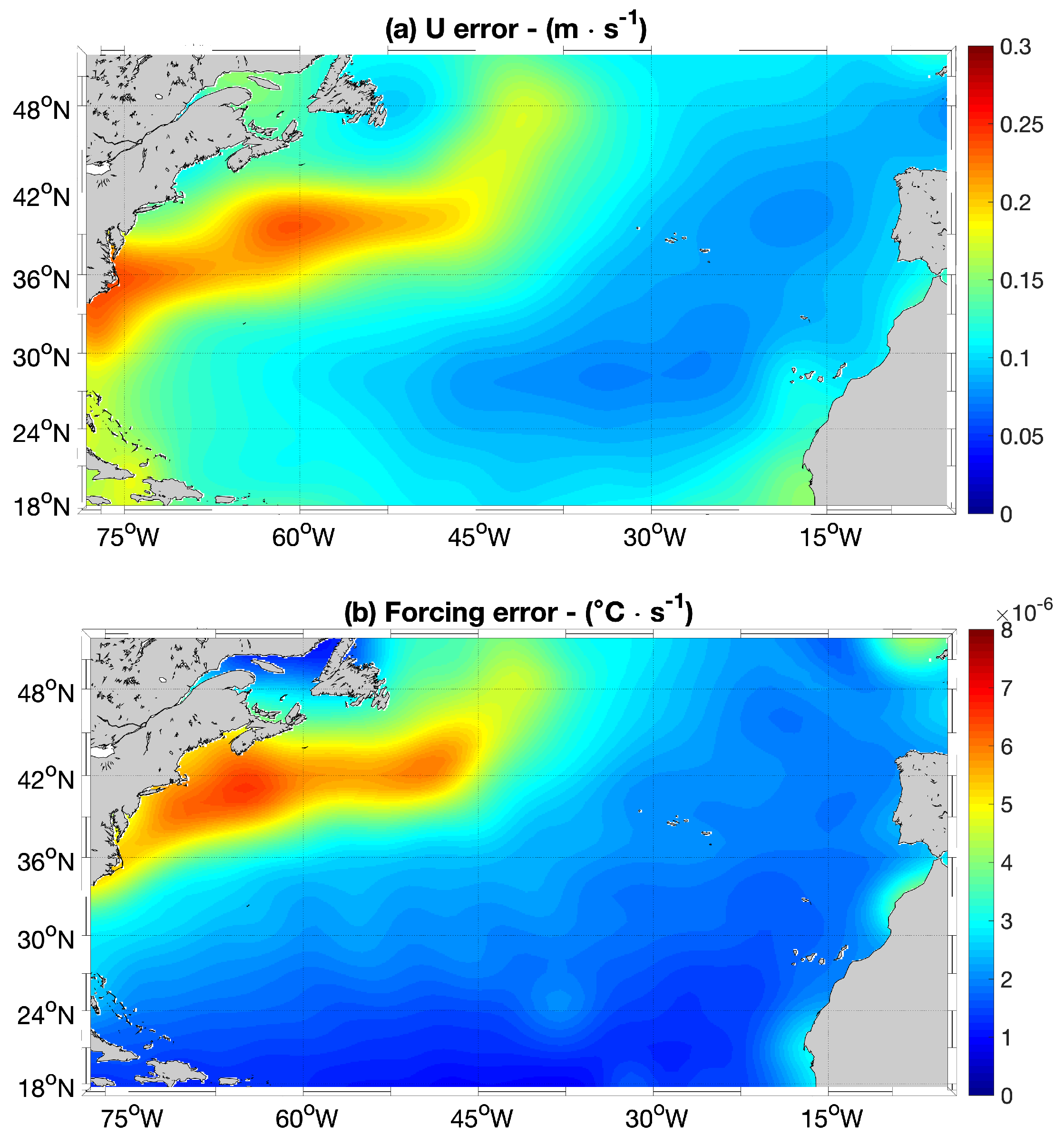
2.5.1. Error on the Geostrophic Currents

The error in the geostrophic currents is crucial to evaluate where the altimeter currents are less accurate, thus enabling us to weight differently the corrections introduced by SST. This computation involved the interpolation of geostrophic currents derived from altimeter data (zonal and meridional components) along the trajectories of NOAA/AOML SVP drogued drifting buoys from 1993 to 2019. Subsequently, the root-mean-square (RMS) error of the geostrophic currents was assessed by considering all interpolated observations into 4° × 4° grids, using SVP currents as a comparative benchmark. To avoid sharp spatial variations resulting from the 4° × 4° binning procedure, a 500 km smoothing process was applied. Figure 1a illustrates an example of the error for the zonal currents ( σ u ). The error is higher in coastal areas and along persistent dynamically active oceanic regions (i.e., the Gulf stream) where it locally reaches 0.25 m/s. This is in agreement with standard altimetry ADT/geostrophic currents formal mapping errors (not shown here) and expresses the fact that gridded, optimally interpolated altimeter-derived data generally suffer from land contamination effects and are characterized by effective spatio-temporal resolutions hindering the description of smaller-scale/fast evolving features (as in highly turbulent areas) [33].

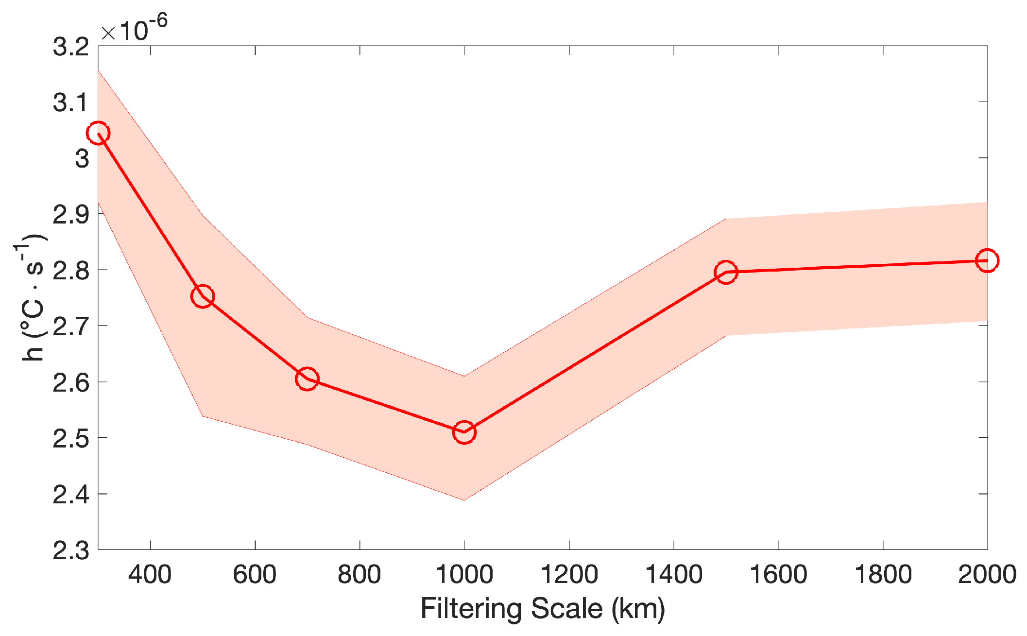
2.5.2. Error in the Forcing Term
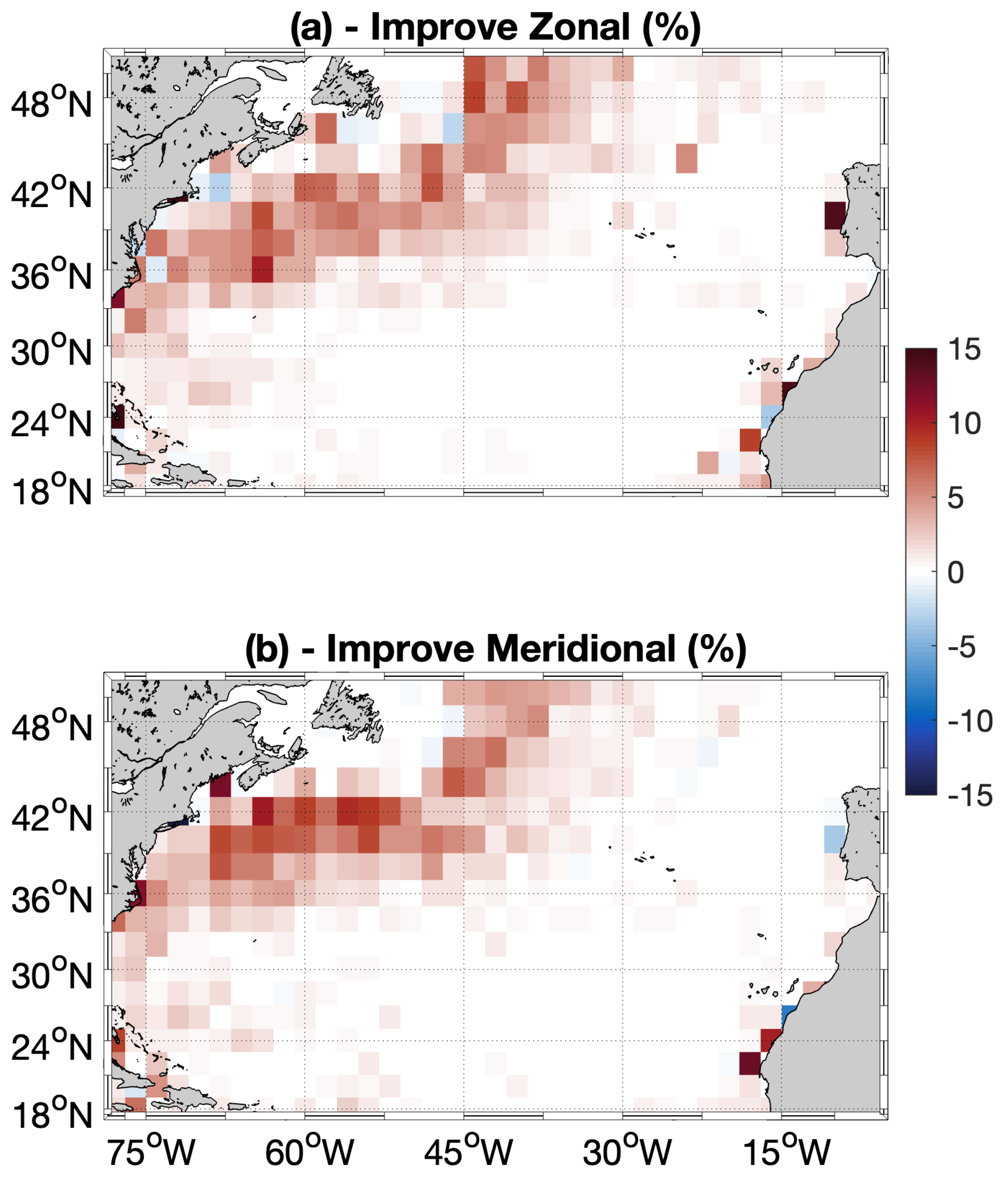
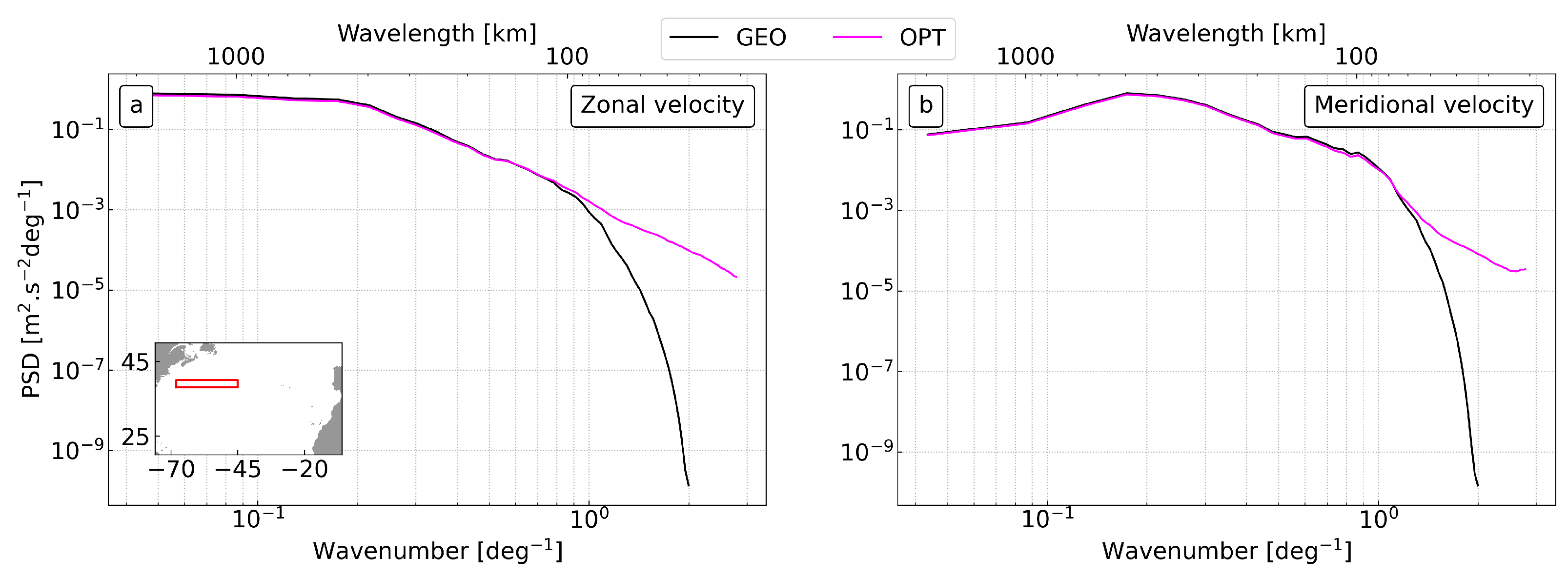
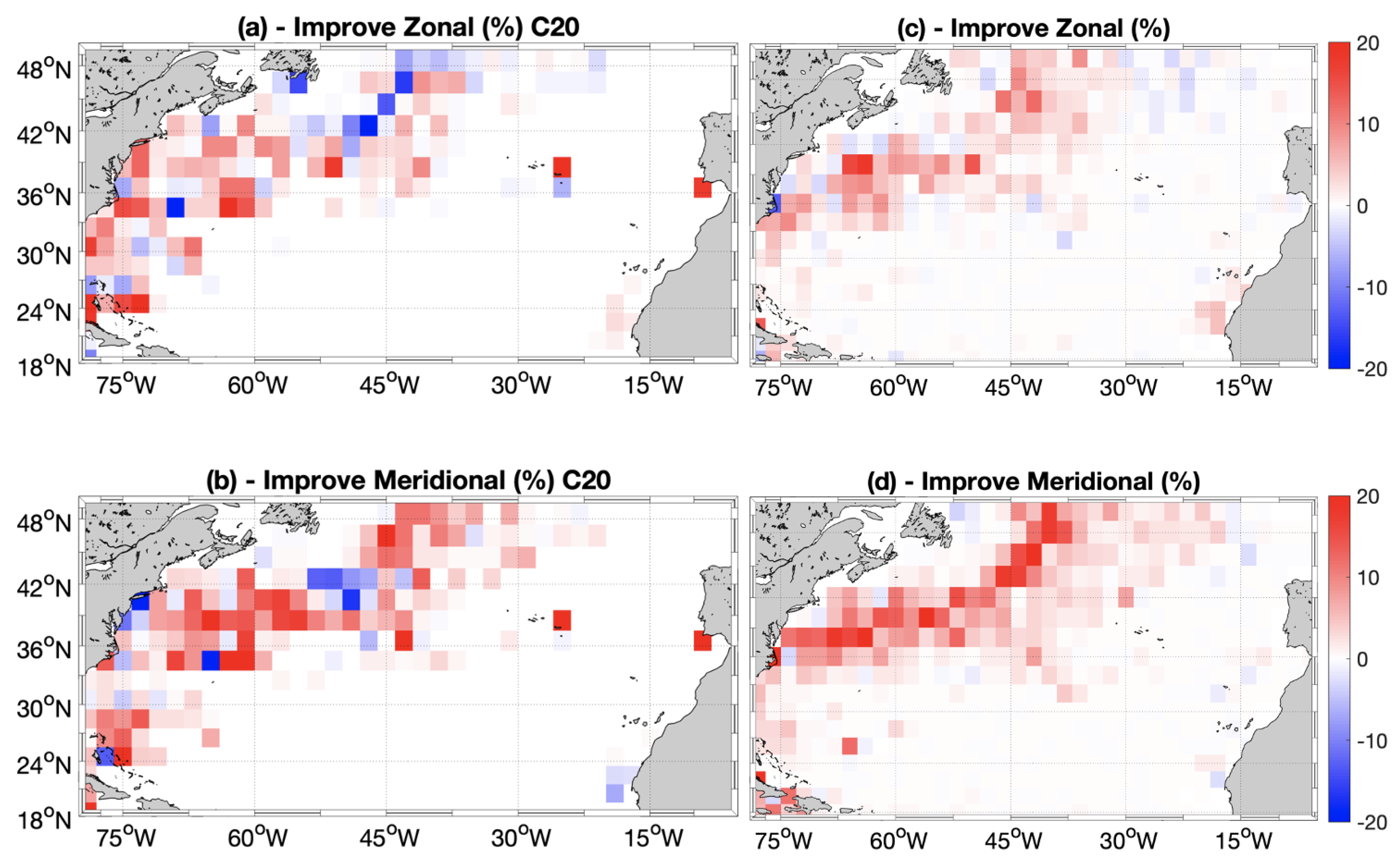
As outlined in [41], the SST Forcing term is mainly identified by the surface heat fluxes, estimated by low-pass spatial filtering of the temporal derivatives of the daily satellite SSTs, as in (6):
F = t SST | L
Here the subscript t denotes the temporal derivative, and L (set to 500 km for global scale applications by [41,49]) stands for the low-pass filtering scale.
To assess the uncertainty associated with such an approximation, we rely on in situ data from drogued SVP drifting buoys. These Lagrangian platforms enable the in situ estimation of the forcing term according to Equation (1). The RMS of the F term is determined by binning the satellite and in situ derived F term into 4° × 4° grids over the period from 1993 to 2019. The resulting error field (also considering the 500 km smoothing) is depicted in Figure 1b.
The filtering scale L appearing in Equation (6) is not expected to be the same across different oceanic basins. For instance, Ref. [60] found a 400 km scale for the Mediterranean area. In the current study, a dedicated analysis was conducted to determine the optimal filtering scale for approximating the F term from the OSTIA t S S T s , utilizing the in situ measured F term obtained from drifting buoys. The in situ measured F, in practice, is obtained considering the buoy-measured surface currents and SSTs in the 1993–2019 period, by means of Equation (1). Over the same period, daily time series of t S S T were generated and low-pass filtered at scales of 200, 300, 500, 1000, 1500, and 2000 km. For each low-pass filtered t S S T time series, an interpolation onto the buoys trajectories was performed as described in Section 2.5. This enabled us to compute the RMS (through the entire study area) between the satellite-derived and the in situ measured F term, presented in Figure 2 as a function of the t S S T filtering scale.
The analyses revealed that the 1000 km filtering scale minimizes discrepancies between the satellite-derived F term and the in situ measured counterpart. Consequently, the OPT surface currents are determined incorporating a forcing term based on t S S T low-pass filtered at 1000 km. The corresponding error map is provided in Figure 1b and, in terms of mean pattern, is in agreement with previous studies ([41]). Finally, as also outlined by [41,49], the error maps were empirically calibrated as illustrated in Appendix A.

3. Results

Initially, we present a test case on 11 July 2018, in the 42°W–40°W and 43°N–45°N bounding box (Figure 3). It illustrates the 2D surface circulation through the following three distinct approaches:
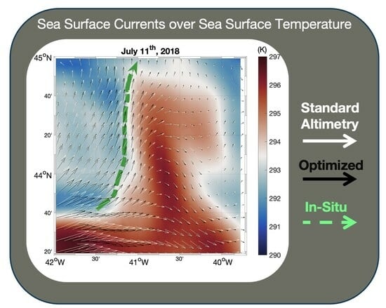
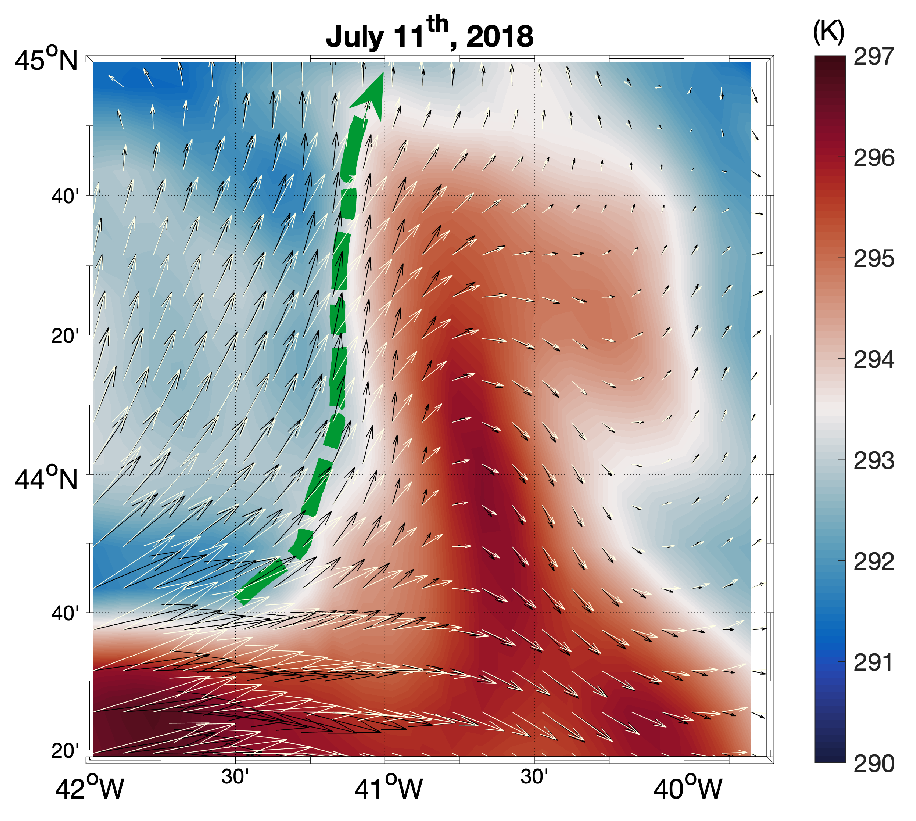
  • The Copernicus Marine altimeter-derived geostrophic currents (depicted by the white arrows);
  • The 2D surface currents derived from the OPT product (represented by black arrows);
  • The trajectory of a drogued drifter, flowing northward along a north–south oceanic surface thermal gradient (green dashed line).
The underlying sea surface temperature is given by the L4 OSTIA SSTs (the ones used to generate the OPT product). The SST pattern depicts an elongated feature characterized by an approximate +2K temperature anomaly relative to the surrounding environment.
The Copernicus Marine geostrophic currents cross the thermal front with angles of up to 45°. For large mesoscale geostrophic flows, if we assume SST plays a dominant role in regulating the surface gradient pressure, such a behaviour is quite unexpected and is presumably due to inaccuracies in the standard altimetry product. On the other hand, the streamlines from the OPT product (black arrows) align well with the pattern of the thermal feature, also exhibiting a good agreement with the trajectory of a drogued drifter (our reference) evolving along the main thermal front on the same date. This example shows how SST can correct the altimeter-derived currents providing a dynamical constraint to improve the description of the geostrophic circulation. The case study is also available online via the World Ocean Circulation visualization tool, accessible via https://odl.bzh/ngvDR7bm (accessed on 25 December 2023).
While this last finding represents a qualitative validation of the OPT currents, a quantitative validation involves the computation of the Percentage of Improvement (PI) relative to standard altimetry, as specified in Equation (7), also following [41].
PI U , V = 100 1 RMS U , V OPT RMS U , V GEO 2
where U and V, respectively, stand for zonal and meridional surface currents. Considering the 2010–2019 period, we performed interpolation of daily GEO and OPT maps onto the trajectories of the SVP, 15 m drogued drifting buoys. The RMS for both altimeter-derived and OPT current estimates were then computed, utilizing the in situ measured currents as a benchmark. The OPT velocities are indeed computed relying on foundation (10 m depth) SSTs. In areas of intense SST gradients, where the corrections from SST are pronounced [41,49], we can expect the OPT estimates to represent currents at 10 m depth, thus making the 15 m drogued drifters a valid reference. By the way, it should be also kept in mind that SVP drifters constitute the standard validation benchmark also for operational altimeter-derived products (e.g., [61]).
The PI was ultimately computed within 2° × 2° spatial bins, considering all available observations within each box. The resulting PI is presented in Figure 4. Consistent with previous studies (e.g., [41,49]), our reconstruction methodology yielded larger improvements in the meridional component of the surface circulation. Local PI values reached 20%, particularly accentuated along the Gulf Stream axis. Furthermore, 67% of the analyzed boxes exhibited PIs larger than zero.
Concerning the zonal component of motion, local improvements fell within the 5–13% range, and boxes with PIs larger than zero covered 69% of the study area. For both components of surface circulation, occasional degradations (i.e., negative PIs) were observed, never exceeding 2%. Notably, most of the larger improvements were concentrated near the Gulf Stream main axis, where the intensified SST gradients resulted in enhanced correction factors according to Equations (3) and (4).
An additional inter comparison of the GEO and OPT products is finally performed through spectral analysis considering the two components (zonal and meridional) of the surface flow. By selecting an area along the axis of the Gulf Stream and employing the Fast Fourier Transform analysis, we quantified the spectral characteristics of the two aforementioned products following a methodology proposed by [41,62] over the entire 2010–2019 time series. At a large scale (>100 km), the power spectral density (PSD) of the two spectra displays a similar pattern, signifying a comparable description of the large mesoscale oceanic features. As we progressively approach smaller scales, approximately from ≃100 km downward (1 deg−1 wavenumber onward), the GEO currents spectrum (black line in Figure 5) rapidly falls towards significantly lower values compared to the OPT one (for both the zonal and the meridional currents), suggesting a less efficient representation of the mesoscale motion in the 100 to 30 km scale. Below scales of 40 km and 30 km, the GEO and OPT datasets, respectively, display spectra dominated by noise (thus excluded from Figure 5).

Comparisons with Respect to Previous Studies

The performances of the OPT currents are here compared to the OPT dataset obtained by [49]. The aim is to show the effect of fine-tuning the ocean currents reconstruction algorithm in the North Atlantic with respect to previous global scale studies based on the same input (first guess) of altimeter-derived geostrophic currents (i.e., the 4SAT case presented in [49]). In [49], the OPT currents were reconstructed and validated by means of Equation (7) in the 2014–2016 period. We thus newly computed the PI of the North Atlantic OPT currents (from the present study) over the same time period and relying on the same validation methodology. The results of [49] (here referred to as C20) are then newly computed over 2° × 2° boxes, leading to the PI depicted in Figure 6a,b for zonal/meridional currents.
In [49], the optimized surface currents dataset exhibited improvements locally reaching 20% for both components of the surface flow, although degradations of the same magnitude were occasionally observed along the Gulf Stream. Interestingly, the validation of the updated optimized currents (from the present-day version of the algorithm) are showing weak degradation, only around −5%, and a more homogeneous improvement pattern along the Gulf Stream.
Focusing on the updated OPT currents, we also performed a significance test to identify areas where the PI shown in Figure 6c,d is statistically significant. To this aim, we followed a procedure based on t-student statistics described in [41]. Such analyses (not shown here) confirmed that the improvement patterns of OPT currents presented in this study are significant with a 95% confidence level.

4. Discussion and Conclusions

Exploiting information from satellite-derived oceanic surface tracers, either alone or in combination with other satellite-derived data, is beneficial for ocean dynamics applications [28,29,39,40,41,46,47,48,49,60,63]. Here, based on previous studies focused on the global-scale surface current reconstruction, we tuned an ocean currents computation methodology in a key geographic region for scientific and practical purposes: the North Atlantic Ocean ([2,52,53,64]).
In the past, such an approach was tested by merging global-scale satellite SSTs and altimeter derived currents with the tentative aim of a near-real time operational production ([49]). The reconstruction methodology was thus tested with different operational SST data and lead to the following main conclusions:
  • Global scale improvements are highly challenging to achieve. This is due to intrinsic issues in the high-latitude SST data, whose quality is severely impacted by cloud cover, preventing an accurate SST retrieval in the InfraRed band and generating degradation when SST data are merged with the altimeter-derived currents.
  • The use of the OSTIA SSTs minimized the occurrences of degradations in the synergistic currents (i.e., merging altimeter and SST data) at high latitude, also exhibiting satisfying performances at low and mid-latitudes.
  • The accurate representation of dynamical features in SST fields, namely the SST gradients associated with the currents advection, is pivotal for a successful implementation of the synergistic ocean currents reconstruction.
Here, the ocean currents reconstruction was performed over a 10-year-long (2010–2019) timescale. There are several reasons behind this choice. Firstly, this study is carried out in the framework of the ESA World Ocean Circulation (WOC) project [65], https://www.worldoceancirculation.org/ (accessed on 19 May 2023)). Among the WOC requirements, the development of space-based observations products had to include contributions from the ESA Earth Explorer 2 SMOS mission, launched back in 2009. The SMOS SSS observations are indeed employed in a WOC product devoted to the 3D ocean currents computation and using information derived from the OPT currents among the input data [66]. A 10 years long time series is also sufficient to ensure robust statistics for the assessment of the generated dataset; the validation carried out by means of Equation (7) and depicted in Figure 4 could rely on an average of O ( 10 3 ) in situ observations in the 2° × 2° boxes. In addition, the 2010–2019 period is characterized by an optimal coverage in terms of available radar altimeters to derive surface geostrophic (first guess) circulation [31]. It also ensures the use of a reprocessed OSTIA SST dataset generated via specific algorithms that maximise feature resolution, guaranteeing a dynamically consistent representation of SST patterns [56,57]. This is an upgrade compared with previous studies, where a near-real-time operational SST product was considered [49]. A quick assessment of the reprocessed OSTIA versus the near real time SST products is also provided in Appendix B.
The percentage of improvement with respect to standard altimeter-derived currents depicts a well-known behaviour of the reconstruction methodology proposed here [41]. The improvement pattern follows the SST spatial gradient intensity distribution in the North Atlantic Ocean, i.e., larger in correspondence of the Gulf Stream and upwelling areas, with peaks of ≃20% and only few degradation occurrences. Improvements are thus found both in coastal areas and the open ocean. However, the 67°W to 45°W–36°N to 43°N region shows no degradation occurrences for both components of the OPT currents (Figure 4), suggesting that our reconstruction methodology is particularly indicated for open ocean contexts.
Following spectral analysis and considering the bounding box depicted in Figure 5a, the GEO and OPT datasets are able to describe oceanographic features until scales of 40 and 30 km, respectively. Below such scales, the spectra evolution is not shown due to the following reasons: (i) The GEO spectrum exhibited nonphysical bumps, very likely due to the upsizing of the native 1/4° data onto the final 1/10° OPT grid. This upsize was specifically carried out to inter-compare the GEO and OPT datasets on the same grids. (ii) The OPT spectrum is characterized by a pretty much flat evolution, basically suggesting the injection of noise at small scales. The inter-comparison of the spectral properties was also repeated remapping the OPT currents onto the 1/4° GEO grid, leading to similar conclusions (not shown). As such, the OPT currents are mainly applicable to the description of the oceanic mesoscale circulation in the North Atlantic region, the latter being characterized by Rossby deformation radii ranging from 15 to 50 km [67].
The OPT dataset thus showed improved performances with respect to standard altimetry both in terms of variability and in the characterization of dynamical features at scales between 100 and 30 km. Such a dataset was prepared to achieve an effective resolution of 1/10°, but spectral analyses confirmed this is very challenging to achieve. The main limitations are very likely due to (i) the use of optimally interpolated (L4) satellite-derived data, whose effective resolutions can be lower than the nominal ones due to the L4 processing (e.g., [33,49]); (ii) the approximations behind the estimate of the forcing terms (Equation (6)), here mainly identified by large-scale surface heat fluxes, which may cause the overlooking of small scale SST variations due to the actual SST source and sink terms, including vertical advection and entrainment velocity; (iii) the use of a smooth noise-robust differentiator for the computation of the SST spatial and temporal derivatives appearing in Equation (5), whose purpose is to minimize occurrences of small-scale noise in the satellite SSTs after the L4 processing, at the cost of reducing sharpness in the SST-related dynamical features. The OPT dataset, despite the aforementioned limitations, constitutes an improved surface geostrophic current estimate compared to present day capabilities and compared to previous studies on the same topic [49], as shown by the results depicted in Figure 6; although, its use is mainly recommended for open ocean and mesoscale dynamics applications. Applications based on the OPT algorithm can span from the scientific domain [54,66] up to the potential implementation for reprocessing past time series of altimeter-derived geostrophic currents.

Author Contributions

Conceptualization, D.C. and B.B.N.; methodology, D.C.; software, D.C. and S.A.; validation, D.C. and S.A.; formal analysis, D.C., B.B.N. and S.A.; investigation, D.C. and B.B.N.; resources, D.C. and B.B.N.; data curation, D.C. and B.B.N.; writing—original draft preparation, D.C.; writing—review and editing, D.C., S.A. and B.B.N.; visualization, D.C. and S.A.; supervision, D.C. and B.B.N.; project administration, D.C. and B.B.N.; funding acquisition, B.B.N. All authors have read and agreed to the published version of the manuscript.

Funding

This research was funded by the European Space Agency through the World Ocean Circulation project (ESA Contract No. 4000130730/20/I-NB/WOC_Subcontract_Odl_CNR).

Data Availability Statement

The altimeter-derived geostrophic (GEO) currents are distributed via the Copernicus Marine Service web portal: https://marine.copernicus.eu/ (accessed on 28 November 2023), accessible upon registration. The optimized (OPT) surface currents are freely available via the ESA World Ocean Circulation Project website: https://www.worldoceancirculation.org/ (accessed on 13 August 2023), DOI: https://doi.org/10.12770/e84fe404-1ed3-4e6f-9b72-f75cd8eb7f7d (accessed on 26 June 2023).

Acknowledgments

We thank the three anonymous Reviewers for providing constructive comments on the manuscript, as well as the ESA-World Ocean Circulation consortium for fruitful discussions on the topic. We also thank Andrea Pisano, Chunxue Yang, Chongyuan Mao and the members of the Group for High Resolution Sea Surface Temperature Task team on Climatology and L4 inter-comparison for the discussions on the satellite SST data.

Conflicts of Interest

The authors declare no conflict of interest.

Abbreviations

The following abbreviations are used in this manuscript:
AOMLAtlantic Oceanographic and Meteorological Laboratory
C3SCopernicus Climate Change Service
CMSCopernicus Marine Service
ENVISATEnvironmental Satellite
ESAEuropean Space Agency
EUMETSATEuropean Organisation for the Exploitation of Meteorological Satellites
CCIClimate Change Initiative
HadIODHadley Centre Integrated Ocean Database
NOAANational Oceanic and Atmospheric Administration
OSI-SAFOcean and Sea Ice - Satellite Application Facility
SVPSurface Velocity Program
T/PTopex/Poseidon
REMSSRemote Sensing Systems
SMOSSoil Moisture and Ocean Salinity
SSSSea Surface Salinity

Appendix A. Empirical Calibration of the Correction Factors

The correction factors, as outlined in Section 2, are strongly dependent on the SST spatial temporal derivatives as well as the SST source/sink terms. After [41,49], the computation of the optimal currents requires a fine tuning of the reconstruction algorithm. To optimize the OPT current performances relative to the altimeter system, the error maps detailed in Section 2.5 necessitate empirical calibration based on in situ data from Lagrangian SVP drogued drifters. This calibration operation influences the set of Equation (5), thereby modulating the correction factors values. The empirical calibration of σ u , v and h was executed by computing three-year-long time series of optimal currents (spanning 2014–2016) using Equations (2)–(5) and applying empirical calibration factors ranging from 1 to 4 in increments of 0.5 for both σ u , v and h. This process resulted in 49 distinct reconstructions for each combination of the calibration factors.
For each reconstruction, the average improvement (expressed as the percentage of improvement, PI) relative to standard altimetry was computed using Equation (7). We recall here that the PI indicates an enhancement of the altimeter-derived currents after the optimal combination with satellite SSTs. Equation (7) enabled to evaluate the mean value of the PI and to detect the areas where the PI exceeded zero, the latter expressed as a fraction of the entire study area.
The calibration factors that maximized both the areas of improvement and their mean value were determined to be 2.5 and 3 for σ u , v and h, respectively, in fair agreement with previous studies [41,49].

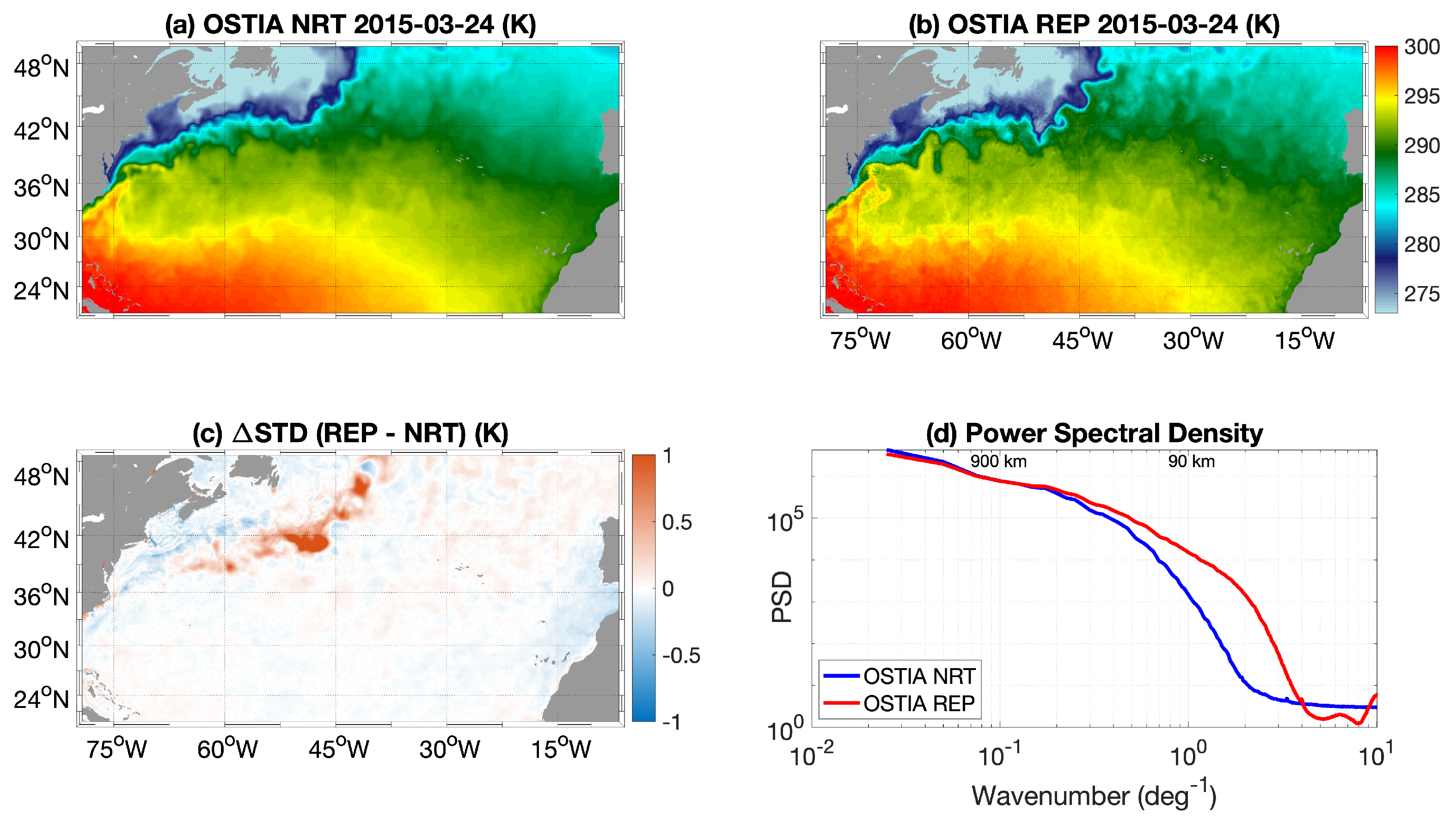
Appendix B. Comparing the Reprocessed and Near Real Time OSTIA SSTs

A comparison of the near-real-time (NRT) versus reprocessed (REP) OSTIA SSTs is provided in Figure A1, showing two snapshot examples on 24 March 2015 (panels (a) and (b)) as well as statistical and spectral analyses based on a one-year-long time series (panels (c) and (d)). The data are accessible via the Copernicus marine service web portal (https://data.marine.copernicus.eu/, accessed on 12 December 2023) under the following product IDs:
  • SST_GLO_SST_L4_NRT_OBSERVATIONS_010_001
  • SST_GLO_SST_L4_REP_OBSERVATIONS_010_011
Figure A1. (a,b) SST from the OSTIA NRT and REP products, respectively, (the maps refer to 24 March 2015); SST from the OSTIA REP product (employed in the present study); (c) STD differences between the REP and NRT products on a one year time scale (2016); (d) spectral analysis for the NRT and REP OSTIA products over 2016, in the bounding box sketched in Figure 5a.
Remotesensing 16 00640 g0a1
After visual inspection of the selected test case, the REP SST field shows a much more detailed description of the SST patterns associated with the mesoscale dynamics in our study area, potentially resulting in a more efficient application to the ocean currents methodology presented here. The higher variability of the reprocessed OSTIA SSTs vs. the NRT ones is also assessed on a one-year-time scale. Randomly choosing one year of our time series (2016), we inter-compared the temporal standard deviations (STD) of the two datasets in our study area. The REP product shows a much larger variability in correspondence with dynamically active areas (i.e., the Gulf Stream), resulting in an enhancement of the STD by about 1K (Figure A1c). Additionally, still choosing the year 2016 and focusing on the bounding box depicted in Figure 5a (inset map), we evaluated the power spectral density of OSTIA NRT and REP, using the same methodology already described in Section 3. For scales larger than ≃ 500 km, the NRT and REP products display a fairly equivalent behaviour. Progressively approaching the mesoscale range, O(100 km), the NRT spectrum (blue line in Figure A1d) drops compared to the REP OSTIA product, suggesting a less efficient representation of the mesoscale features in the NRT L4 SSTs. Eventually, the REP and NRT SSTs spectra indicate noise below the respective scales of ≃40 km and ≃20 km, as suggested by the flattening of the spectra. A thorough comparison of OSTIA REP and NRT datasets is out of scope for the present study. Nevertheless, such analyses suggest a positive impact of the REP dataset (compared to the NRT one) for dynamical applications as the one addressed in the present study.

References

  1. Merino, M.; Monreal-Gómez, M. Ocean currents and their impact on marine life. In Marine Ecology; EOLSS Publications: Oxford, UK, 2009; pp. 47–52. [Google Scholar]
  2. Zaccone, R.; Ottaviani, E.; Figari, M.; Altosole, M. Ship voyage optimization for safe and energy-efficient navigation: A dynamic programming approach. Ocean Eng. 2018, 153, 215–224. [Google Scholar] [CrossRef]
  3. Onink, V.; Wichmann, D.; Delandmeter, P.; Van Sebille, E. The role of Ekman currents, geostrophy, and Stokes drift in the accumulation of floating microplastic. J. Geophys. Res. Ocean. 2019, 124, 1474–1490. [Google Scholar] [CrossRef] [PubMed]
  4. Comby, C.; Petrenko, A.; Estournel, C.; Marsaleix, P.; Ulses, C.; Bosse, A.; Doglioli, A.; Barrillon, S. Near Inertial Oscillations and Vertical Velocities Modulating Phytoplankton After a Storm in the Mediterranean Sea. J. Water Resour. Ocean Sci. 2023, 12, 31–37. [Google Scholar] [CrossRef]
  5. Bashmachnikov, I.; Neves, F.; Calheiros, T.; Carton, X. Properties and pathways of Mediterranean water eddies in the Atlantic. Prog. Oceanogr. 2015, 137, 149–172. [Google Scholar] [CrossRef]
  6. Barbosa Aguiar, A.C.; Peliz, Á.; Carton, X. A census of Meddies in a long-term high-resolution simulation. Prog. Oceanogr. 2013, 116, 80–94. [Google Scholar] [CrossRef]
  7. Chenillat, F.; Franks, P.J.; Combes, V. Biogeochemical properties of eddies in the California Current System. Geophys. Res. Lett. 2016, 43, 5812–5820. [Google Scholar] [CrossRef]
  8. Siokou-Frangou, I.; Christaki, U.; Mazzocchi, M.G.; Montresor, M.; Ribera d’Alcalá, M.; Vaqué, D.; Zingone, A. Plankton in the open Mediterranean Sea: A review. Biogeosciences 2010, 7, 1543–1586. [Google Scholar] [CrossRef]
  9. Carlson, D.F.; Clarke, A.J. Seasonal along-isobath geostrophic flows on the west Florida shelf with application to Karenia brevis red tide blooms in Florida’s Big Bend. Cont. Shelf Res. 2009, 29, 445–455. [Google Scholar]
  10. Buongiorno Nardelli, B. Vortex waves and vertical motion in a mesoscale cyclonic eddy. J. Geophys. Res. Ocean. 2013, 118, 5609–5624. [Google Scholar] [CrossRef]
  11. Stephens, J.C.; Marshall, D.P. Dynamics of the Mediterranean salinity tongue. J. Phys. Oceanogr. 1999, 29, 1425–1441. [Google Scholar] [CrossRef]
  12. Grech, A.; Wolter, J.; Coles, R.; McKenzie, L.; Rasheed, M.; Thomas, C.; Waycott, M.; Hanert, E. Spatial patterns of seagrass dispersal and settlement. Divers. Distrib. 2016, 22, 1150–1162. [Google Scholar] [CrossRef]
  13. Jian, Z.; Yu, J.; Wang, Y.; Dang, H.; Dai, M.; Li, C.; Ji, X.; Wang, X.; Chen, Y. Equatorial Pacific Sea-Air CO2 Exchange Modulated by Upper Ocean Circulation During the Last Deglaciation. Geophys. Res. Lett. 2023, 50, e2023GL105169. [Google Scholar] [CrossRef]
  14. Ribotti, A.; Bussani, A.; Menna, M.; Satta, A.; Sorgente, R.; Cucco, A.; Gerin, R. A Mediterranean drifter dataset. Earth Syst. Sci. Data 2023, 15, 4651–4659. [Google Scholar] [CrossRef]
  15. Menna, M.; Poulain, P.M.; Bussani, A.; Gerin, R. Detecting the drogue presence of SVP drifters from wind slippage in the Mediterranean Sea. Measurement 2018, 125, 447–453. [Google Scholar] [CrossRef]
  16. Laurindo, L.C.; Mariano, A.J.; Lumpkin, R. An improved near-surface velocity climatology for the global ocean from drifter observations. Deep Sea Res. Part I Oceanogr. Res. Pap. 2017, 124, 73–92. [Google Scholar] [CrossRef]
  17. Poulain, P.M.; Menna, M.; Mauri, E. Surface geostrophic circulation of the Mediterranean Sea derived from drifter and satellite altimeter data. J. Phys. Oceanogr. 2012, 42, 973–990. [Google Scholar] [CrossRef]
  18. Teague, C.C.; Vesecky, J.F.; Hallock, Z.R. A comparison of multifrequency HF radar and ADCP measurements of near-surface currents during COPE-3. IEEE J. Ocean. Eng. 2001, 26, 399–405. [Google Scholar] [CrossRef]
  19. Beardsley, R.; Boicourt, W.; Huff, L.; McCullough, J.; Scott, J. CMICE: A near-surface current meter intercomparison experiment. Deep Sea Res. Part A Oceanogr. Res. Pap. 1981, 28, 1577–1603. [Google Scholar] [CrossRef]
  20. Capodici, F.; Cosoli, S.; Ciraolo, G.; Nasello, C.; Maltese, A.; Poulain, P.M.; Drago, A.; Azzopardi, J.; Gauci, A. Validation of HF radar sea surface currents in the Malta-Sicily Channel. Remote Sens. Environ. 2019, 225, 65–76. [Google Scholar] [CrossRef]
  21. Drago, A.; Ciraolo, G.; Capodici, F.; Cosoli, S.; Gacic, M.; Poulain, P.; Tarasova, R.; Azzopardi, J.; Gauci, A.; Maltese, A.; et al. CALYPSO? An operational network of HF radars for the Malta-Sicily Channel. In Proceedings of the 7th International Conference on EuroGOOS, Lisbon, Portugal, 28–30 October 2014; Eurogoos Publication: Brussels, Belgium, 2015; Volume 30, pp. 28–30. [Google Scholar]
  22. Chapron, B.; Collard, F.; Ardhuin, F. Direct measurements of ocean surface velocity from space: Interpretation and validation. J. Geophys. Res. Ocean. 2005, 110. [Google Scholar] [CrossRef]
  23. Madec, G.; Bourdallé-Badie, R.; Bouttier, P.A.; Bricaud, C.; Bruciaferri, D.; Calvert, D.; Chanut, J.; Clementi, E.; Coward, A.; Delrosso, D.; et al. NEMO Ocean Engine. 2017. Available online: https://www.nemo-ocean.eu/doc/ (accessed on 19 May 2023).
  24. Jean-Michel, L.; Eric, G.; Romain, B.B.; Gilles, G.; Angélique, M.; Marie, D.; Clément, B.; Mathieu, H.; Olivier, L.G.; Charly, R.; et al. The Copernicus global 1/12 oceanic and sea ice GLORYS12 reanalysis. Front. Earth Sci. 2021, 9, 698876. [Google Scholar] [CrossRef]
  25. Pascual, A.; Faugère, Y.; Larnicol, G.; Le Traon, P.Y. Improved description of the ocean mesoscale variability by combining four satellite altimeters. Geophys. Res. Lett. 2006, 33. [Google Scholar] [CrossRef]
  26. Fu, L.L.; Chelton, D.B.; Zlotnicki, V. Satellite altimetry: Observing ocean variability from space. Oceanography 1988, 1, 4–58. [Google Scholar] [CrossRef]
  27. Pujol, M.I.; Dibarboure, G.; Le Traon, P.Y.; Klein, P. Using high-resolution altimetry to observe mesoscale signals. J. Atmos. Ocean. Technol. 2012, 29, 1409–1416. [Google Scholar] [CrossRef]
  28. Qazi, W.A.; Emery, W.J.; Fox-Kemper, B. Computing ocean surface currents over the coastal California current system using 30-min-lag sequential SAR images. IEEE Trans. Geosci. Remote Sens. 2014, 52, 7559–7580. [Google Scholar] [CrossRef]
  29. Bowen, M.M.; Emery, W.J.; Wilkin, J.L.; Tildesley, P.C.; Barton, I.J.; Knewtson, R. Extracting multiyear surface currents from sequential thermal imagery using the maximum cross-correlation technique. J. Atmos. Ocean. Technol. 2002, 19, 1665–1676. [Google Scholar] [CrossRef]
  30. Abdalla, S.; Kolahchi, A.A.; Ablain, M.; Adusumilli, S.; Bhowmick, S.A.; Alou-Font, E.; Amarouche, L.; Andersen, O.B.; Antich, H.; Aouf, L.; et al. Altimetry for the future: Building on 25 years of progress. Adv. Space Res. 2021, 68, 319–363. [Google Scholar] [CrossRef]
  31. Taburet, G.; Sanchez-Roman, A.; Ballarotta, M.; Pujol, M.I.; Legeais, J.F.; Fournier, F.; Faugere, Y.; Dibarboure, G. DUACS DT2018: 25 years of reprocessed sea level altimetry products. Ocean Sci. 2019, 15, 1207–1224. [Google Scholar] [CrossRef]
  32. Vallis, G.K. Atmospheric and Oceanic Fluid Dynamics; Cambridge University Press: Cambridge, UK, 2006; p. 745. [Google Scholar]
  33. Ballarotta, M.; Ubelmann, C.; Pujol, M.I.; Taburet, G.; Fournier, F.; Legeais, J.F.; Faugère, Y.; Delepoulle, A.; Chelton, D.; Dibarboure, G.; et al. On the resolutions of ocean altimetry maps. Ocean Sci. 2019, 15, 1091–1109. [Google Scholar] [CrossRef]
  34. Fu, L.; Alsdorf, D.; Rodriguez, E.; Morrow, R.; Mognard, N.; Lambin, J.; Vaze, P.; Lafon, T. The SWOT (Surface Water and Ocean Topography) Mission: Spaceborne Radar Interferometry for Oceanographic and Hhydrological Applications. In Proceedings of the OCEANOBS, Venice, Italy, 21–25 September 2009. [Google Scholar]
  35. Morrow, R.; Fu, L.L.; Ardhuin, F.; Benkiran, M.; Chapron, B.; Cosme, E.; d’Ovidio, F.; Farrar, J.T.; Gille, S.T.; Lapeyre, G.; et al. Global observations of fine-scale ocean surface topography with the surface water and ocean topography (SWOT) mission. Front. Mar. Sci. 2019, 6, 232. [Google Scholar] [CrossRef]
  36. Morrow, R.; Fu, L.L.; Rio, M.H.; Ray, R.; Prandi, P.; Le Traon, P.Y.; Benveniste, J. Ocean circulation from space. Surv. Geophys. 2023, 44, 1243–1286. [Google Scholar] [CrossRef]
  37. Ubelmann, C.; Klein, P.; Fu, L.L. Dynamic interpolation of sea surface height and potential applications for future high-resolution altimetry mapping. J. Atmos. Ocean. Technol. 2015, 32, 177–184. [Google Scholar] [CrossRef]
  38. Mulet, S.; Etienne, H.; Ballarotta, M.; Faugere, Y.; Rio, M.; Dibarboure, G.; Picot, N. Synergy between surface drifters and altimetry to increase the accuracy of sea level anomaly and geostrophic current maps in the Gulf of Mexico. Adv. Space Res. 2020, 68, 420–431. [Google Scholar] [CrossRef]
  39. González-Haro, C.; Isern-Fontanet, J. Global ocean current reconstruction from altimetric and microwave SST measurements. J. Geophys. Res. Ocean. 2014, 119, 3378–3391. [Google Scholar] [CrossRef]
  40. Rio, M.H.; Santoleri, R.; Bourdalle-Badie, R.; Griffa, A.; Piterbarg, L.; Taburet, G. Improving the Altimeter-Derived Surface Currents Using High-Resolution Sea Surface Temperature Data: A Feasability Study Based on Model Outputs. J. Atmos. Ocean. Technol. 2016, 33, 2769–2784. [Google Scholar] [CrossRef]
  41. Rio, M.H.; Santoleri, R. Improved global surface currents from the merging of altimetry and Sea Surface Temperature data. Remote Sens. Environ. 2018, 216, 770–785. [Google Scholar] [CrossRef]
  42. Bingham, R.J.; Knudsen, P.; Andersen, O.B. Estimating the North Atlantic mean dynamic topography and geostrophic currents with GOCE. In Proceedings of the 4th International GOCE User Workshop, Munich, Germany, 31 March–1 April 2011; European Space Agency: Paris, France, 2011. [Google Scholar]
  43. Knudsen, P.; Andersen, O.; Maximenko, N. A new ocean mean dynamic topography model, derived from a combination of gravity, altimetry and drifter velocity data. Adv. Space Res. 2021, 68, 1090–1102. [Google Scholar] [CrossRef]
  44. Vargas-Alemañy, J.A.; Vigo, M.I.; García-García, D.; Zid, F. Updated geostrophic circulation and volume transport from satellite data in the Southern Ocean. Front. Earth Sci. 2023, 11, 1110138. [Google Scholar] [CrossRef]
  45. Buongiorno Nardelli, B.; Cavaliere, D.; Charles, E.; Ciani, D. Super-resolving ocean dynamics from space with computer vision algorithms. Remote Sens. 2022, 14, 1159. [Google Scholar] [CrossRef]
  46. Martin, S.A.; Manucharyan, G.E.; Klein, P. Synthesizing sea surface temperature and satellite altimetry observations using deep learning improves the accuracy and resolution of gridded sea surface height anomalies. J. Adv. Model. Earth Syst. 2023, 15, e2022MS003589. [Google Scholar]
  47. Beauchamp, M.; Febvre, Q.; Georgenthum, H.; Fablet, R. 4DVarNet-SSH: End-to-end learning of variational interpolation schemes for nadir and wide-swath satellite altimetry. Geosci. Model Dev. Discuss. 2022, 16, 2119–2147. [Google Scholar] [CrossRef]
  48. Fablet, R.; Febvre, Q.; Chapron, B. Multimodal 4DVarNets for the reconstruction of sea surface dynamics from SST-SSH synergies. IEEE Trans. Geosci. Remote Sens. 2023. [Google Scholar] [CrossRef]
  49. Ciani, D.; Rio, M.H.; Buongiorno Nardelli, B.; Etienne, H.; Santoleri, R. Improving the altimeter-derived surface currents using sea surface temperature (SST) data: A sensitivity study to SST products. Remote Sens. 2020, 12, 1601. [Google Scholar] [CrossRef]
  50. Piterbarg, L.I. A simple method for computing velocities from tracer observations and a model output. Appl. Math. Model. 2009, 33, 3693–3704. [Google Scholar] [CrossRef]
  51. Mercatini, A.; Griffa, A.; Piterbarg, L.; Zambianchi, E.; Magaldi, M.G. Estimating surface velocities from satellite data and numerical models: Implementation and testing of a new simple method. Ocean Model. 2010, 33, 190–203. [Google Scholar] [CrossRef]
  52. Deser, C.; Blackmon, M.L. Surface climate variations over the North Atlantic Ocean during winter: 1900–1989. J. Clim. 1993, 6, 1743–1753. [Google Scholar] [CrossRef]
  53. Chang, Y.L.K.; Feunteun, E.; Miyazawa, Y.; Tsukamoto, K. New clues on the Atlantic eels spawning behavior and area: The Mid-Atlantic Ridge hypothesis. Sci. Rep. 2020, 10, 15981. [Google Scholar] [CrossRef]
  54. Munk, P.; Nardelli, B.B.; Mariani, P.; Bendtsen, J. Mesoscale-driven dispersion of early life stages of European eel. Front. Mar. Sci. 2023, 10, 1163125. [Google Scholar] [CrossRef]
  55. GHRSST Science Team. The Recommended GHRSST Data Specification (GDS) 2.0 Document Revision 4; GHRSST International Project Office: Department of Meteorology, University of Reading: Reading UK, 2011. [Google Scholar]
  56. Good, S.; Fiedler, E.; Mao, C.; Martin, M.J.; Maycock, A.; Reid, R.; Roberts-Jones, J.; Searle, T.; Waters, J.; While, J.; et al. The Current Configuration of the OSTIA System for Operational Production of Foundation Sea Surface Temperature and Ice Concentration Analyses. Remote Sens. 2020, 12, 720. [Google Scholar] [CrossRef]
  57. Fiedler, E.; Mao, C.; Good, S.; Waters, J.; Martin, M. Improvements to feature resolution in the OSTIA sea surface temperature analysis using the NEMOVAR assimilation scheme. Q. J. R. Meteorol. Soc. 2019, 145, 3609–3625. [Google Scholar] [CrossRef]
  58. Mulet, S.; Rio, M.H.; Etienne, H.; Artana, C.; Cancet, M.; Dibarboure, G.; Feng, H.; Husson, R.; Picot, N.; Provost, C.; et al. The new CNES-CLS18 global mean dynamic topography. Ocean Sci. 2021, 17, 789–808. [Google Scholar] [CrossRef]
  59. Lumpkin, R.; Grodsky, S.A.; Centurioni, L.; Rio, M.H.; Carton, J.A.; Lee, D. Removing spurious low-frequency variability in drifter velocities. J. Atmos. Ocean. Technol. 2013, 30, 353–360. [Google Scholar] [CrossRef]
  60. Ciani, D.; Rio, M.H.; Menna, M.; Santoleri, R. A Synergetic Approach for the Space-Based Sea Surface Currents Retrieval in the Mediterranean Sea. Remote Sens. 2019, 11, 1285. [Google Scholar] [CrossRef]
  61. Pujol, M.I.; Faugère, Y.; Taburet, G.; Dupuy, S.; Pelloquin, C.; Ablain, M.; Picot, N. DUACS DT2014: The new multi-mission altimeter data set reprocessed over 20 years. Ocean Sci. 2016, 12, 1067–1090. [Google Scholar] [CrossRef]
  62. Droghei, R.; Buongiorno Nardelli, B.; Santoleri, R. A new global sea surface salinity and density dataset from multivariate observations (1993–2016). Front. Mar. Sci. 2018, 5, 84. [Google Scholar] [CrossRef]
  63. Warren, M.; Quartly, G.; Shutler, J.; Miller, P.; Yoshikawa, Y. Estimation of ocean surface currents from maximum cross correlation applied to GOCI geostationary satellite remote sensing data over the Tsushima (Korea) Straits. J. Geophys. Res. Ocean. 2016, 121, 6993–7009. [Google Scholar] [CrossRef]
  64. Kleckner, R.; McCleave, J. Spatial and temporal distribution of American eel larvae in relation to North Atlantic Ocean current systems. Dana 1985, 4, 67–92. [Google Scholar]
  65. Larnicol, G.; Collard, F.; Gaultier, L.; Buongiorno Nardelli, B.; Ciani, D.; Ubelmann, C.; Autret, E.; Piolle, J.F.; Chapron, B.; Moiseev, A.; et al. World Ocean Circulation Project: Retrieve the Ocean Velocities at the Right Place at the Righ Time; European Space Agency: Paris, France, 2022. [Google Scholar]
  66. Asdar, S.; Ciani, D.; Buongiorno Nardelli, B. 3D reconstruction of horizontal and vertical quasi-geostrophic currents in the North Atlantic Ocean. Earth Syst. Sci. Data Discuss. 2023, 2023, 1–29. [Google Scholar]
  67. Chelton, D.; De Szoeke, R.; Schlax, M.; El Naggar, K.; Siwertz, N. Geographical Variability of the First Baroclinic Rossby Radius of Deformation. J. Phys. Oceanogr. 1998, 28, 433–459. [Google Scholar] [CrossRef]
Figure 1. (a) Uncertainty in the zonal geostrophic currents (identified as σ u in Equation (5)). (b) Uncertainty in the Forcing term (identified as “h” in Equation (5)).
Remotesensing 16 00640 g001
Figure 2. Error on the Forcing term as a function of the t SST spatial low-pass filtering scale. The shadowed area indicates the uncertainty on the mean value evaluated via the bootstrap technique.
Remotesensing 16 00640 g002
Figure 3. Intercomparison of standard altimetry geostrophic currents (white arrows) and OPT currents (black arrows) on top of the OSTIA sea surface temperature (11 July 2018). The map also shows the trajectory of a Coriolis drifter drogued at 15 m (dashed green line).
Remotesensing 16 00640 g003
Figure 4. (a) Percentage of improvement computed via Equation (7) in 2° × 2° boxes, for the zonal optimal currents. (b) Same as (a), for the meridional currents. The statistics are computed over the 2010–2019 period.
Remotesensing 16 00640 g004
Figure 5. Power Spectral Density of the GEO (black) and OPT (magenta) currents over the 2010–2019 period, computed in the red box shown in the inset map. Panels (a,b) stand for zonal and meridional flows.
Remotesensing 16 00640 g005
Figure 6. (a) Percentage of improvement (PI) computed via Equation (7) in 2° × 2° boxes, for the zonal optimal currents from [49] (C20). (b) Same as (a), for the meridional currents from [49] (C20). Panels (c,d) refer to the PI of the North Atlantic OPT currents computed over 2014–2016 for zonal and meridional currents, respectively.
Remotesensing 16 00640 g006
Table 1. Summary table of the dataset used in the present study. (N) stands for nominal.
DATAGeostrophic CurrentsSea Surface TemperatureIn-Situ Currents/SST
Spatial Resolution (N)0.25°0.05°sparse
Temporal Resolution (N)dailydailysix-hourly
SourceSatellite (multi-imission)Satellite (multi-mission)Drifting Buoy
AccessCMS portalCMS portalNOAA/AOML portal
Disclaimer/Publisher’s Note: The statements, opinions and data contained in all publications are solely those of the individual author(s) and contributor(s) and not of MDPI and/or the editor(s). MDPI and/or the editor(s) disclaim responsibility for any injury to people or property resulting from any ideas, methods, instructions or products referred to in the content.

