Using a Combination of High-Frequency Coastal Radar Dataset and Satellite Imagery to Study the Patterns Involved in the Coastal Countercurrent Events in the Gulf of Cadiz

Abstract

This study exploits the combination of High-Frequency Coastal Radar (HFR) information with satellite-derived observations to characterize the patterns involved in the coastal countercurrents (CCCs) events in the Gulf of Cadiz (GoC), which is situated in the SW of the Iberian Peninsula. The westward alongshore currents are observed throughout the year, but the main drivers necessary to develop this flow and its extension in both parts of the basin are not fully clear. In order to identify the main physical processes (both local and remote) that induce the development of these countercurrents and to evaluate the connection of the circulation patterns between the eastern and the western part of the GoC, we make use of several data sources available for the region. First of all, a land-based system of HFR antennas located at four different sites of the GoC provides the velocity field of the surface circulation of the basin. To achieve a significant characterization of the CCCs in the Gulf, the dataset analyzed is processed by means of a series of operations, including the Empirical Orthogonal Functions (EOFs) analysis used to identify spatial and temporal variability of the flow, a low-pass filter used to isolate the sub-inertial signal of the current and temporal interpolation to fill in the missing values. Secondly, given the known importance of the zonal component of the local winds combined with the variations in the mean pressure at sea level over the Western Mediterranean during these events, time series of meteorological data are processed and correlated with the current velocity series via a statistical analysis. Finally, sea surface temperature fields and chlorophyll-a distribution patterns are used as tracers to obtain information on the extension of the countercurrents where HFR data are missing in four cases studied during the year 2017. The conducted analysis revealed the consistent occurrence of westward coastal currents throughout the year, driven in the most intense cases by a combination of the zonal component of the local wind and atmospheric pressure fluctuations over the Western Mediterranean Sea. During those events, CCCs reached the Portuguese side of the Gulf and facilitated the advection of biological material and warmer waters.

1. Introduction

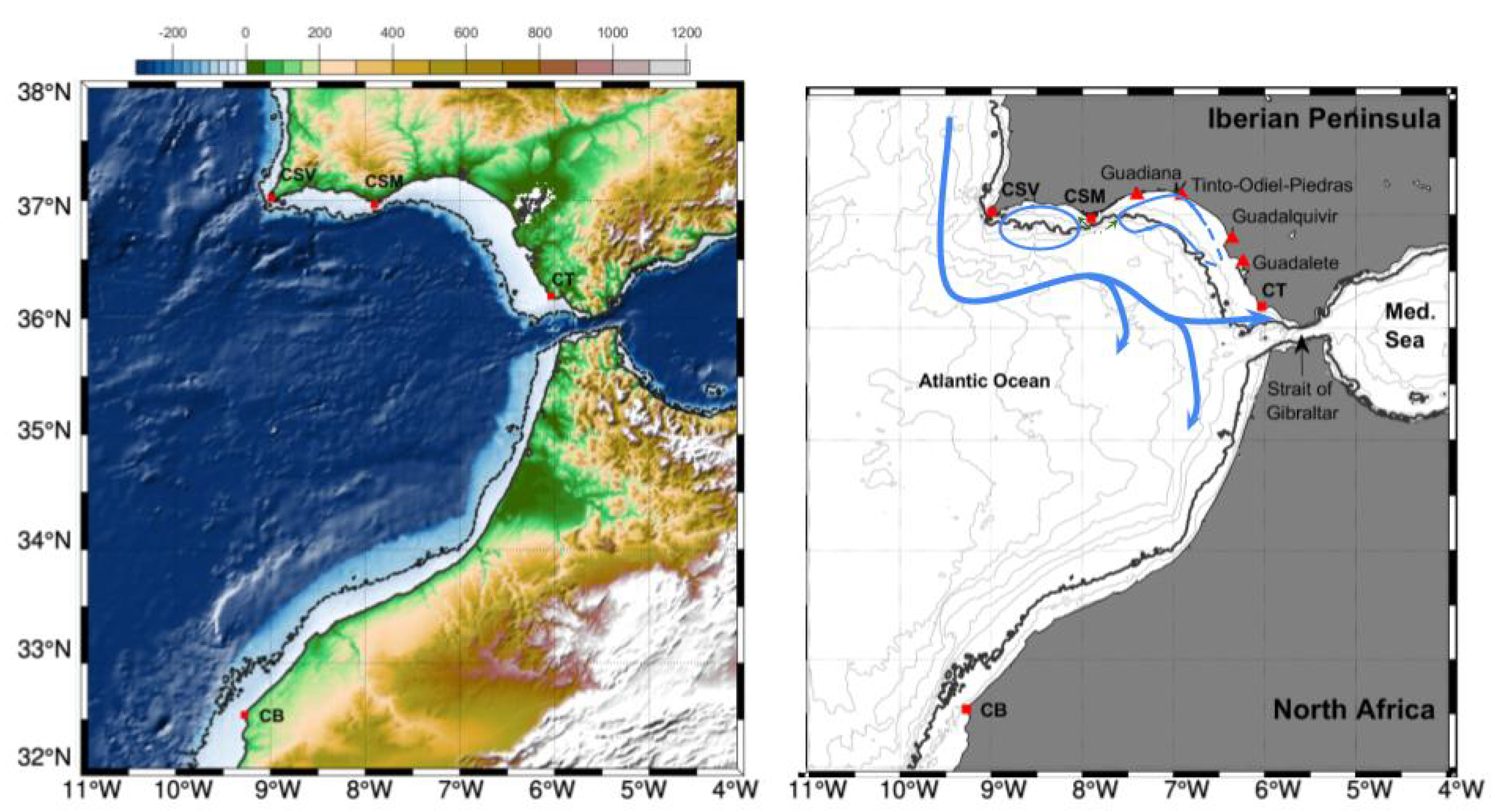
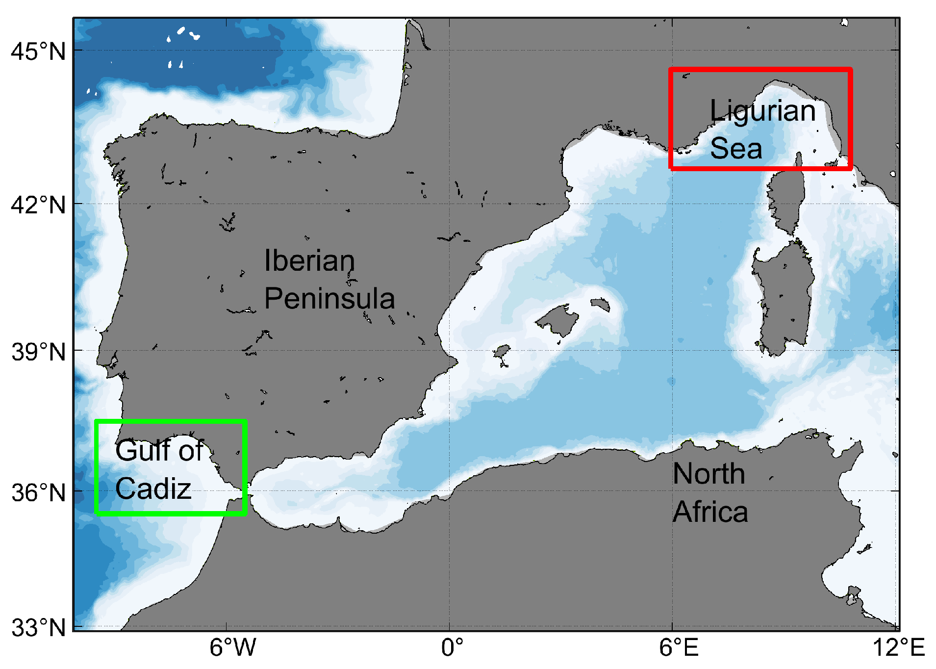
1.1. Geographical Frame

The Gulf of Cadiz (GoC) is the basin located between the south-west of the Iberian peninsula and the north-west of the African coast up to Cape Beddouzza (CB) that connects the North Atlantic with the Mediterranean Sea through the Strait of Gibraltar, its eastern limit. The western limit, the only one not well defined, is usually situated along the 9°W meridian that crosses Cape San Vicente (CSV), located in the extreme south-west of Portugal (Figure 1).

Due to its location, the Gulf presents very complex oceanographic characteristics and its surface dynamics are influenced by several factors. Firstly, the water mass exchange and mixing between the Atlantic Ocean and the Mediterranean Sea play the most important role in the dynamical features of the area and have been extensively explored in the literature (e.g., [1,2,3,4,5,6]). The quasi-stationary two-layer exchange of water masses between the eastern and western part of the Strait is able to compensate the negative water balance of the Mediterranean basin, whose losses due to evaporation exceed the sum of fluvial inputs and precipitation [7]. Secondly, the surface circulation is affected by the influence of the North Atlantic subtropical gyre of the Azores current, which may generate in association with the Mediterranean outflow according to the so-called $\beta$-plume theories [3,4,8]. Finally, the Gulf receives a substantial contribution in terms of fresh waters and dissolved and suspended substances from major rivers of the continent, such as Guadalete, Guadalquivir, Guadiana and Tinto–Odiel–Piedras. Their considerable importance has been widely shown not only by means of their direct impact on nearshore hydrography, but also by proving their influence on the biological productivity of the area [9,10].

Moreover, it is worth mentioning that the Gulf presents several topographic features which play a crucial role in defining the oceanographic regime in the area. On one hand, three capes have a remarkable impact on the physical and biological dynamics of the zone: the above-mentioned Cape San Vicente, where the western and southern coasts of Iberia intersect at almost right angles; Cape Santa María (CSM), which separate the Gulf into two sub-basins that we can identify based on the eastern and western part of the continental shelf; and Cape Trafalgar (CT), which is the closest to the Strait of Gibraltar and is known for being one of the most chlorophyll-rich areas of the Gulf [11]. On the other hand, several important sills, including the Portimao canyon and the Camarinal and Espartel sills, affect the general pattern of the flow in the Gulf of Cadiz, causing instability and vertical mixing [12,13,14].

1.2. Surface Circulation

Due to the unique characteristics of the position of the Gulf, which is a continuous witness of the Mediterranean and the Atlantic waters exchange, many hydrodynamical and meteorological events contribute to define currents regimes and primary production levels in the area. Moreover, the fact that the continental shelf is delimited by the 100 m isoline, which is very close to the coast in proximity of Cape Santa Maria, causes a natural division between the east and the west part of the GoC in terms of dynamical features (see the right panel of Figure 1).

In general, the surface circulation is characterized by an anticyclonic eastward flow in the central part of the basin and westward countercurrents forming cyclone cells above the platform and the open ocean [15]. However, seasonality plays a crucial role in the generation of alternating regimes and, in order to carry out a comprehensive study of surface circulation in the GoC, it is important to understand the effects of the main meteorological factors, both local and remote, coupled with the particular morphology of the southern coast of the Iberian peninsula [16].

The seasonal fluctuations of the North Atlantic subtropical gyre, caused by the displacement of the Azores atmospheric high and by changes in the large-scale wind patterns, affect the nature of the circulation out of the continental shelf in the Gulf of Cadiz, which follows an anticyclonic pattern in summer and cyclonic dynamics in short winter periods [17]. Similar to other regions characterized by coastal upwelling induced by favorable winds, the GoC usually shows an alongshore circulation aligned with the wind direction. Typically, the flow entering the Gulf forks in two ways: on one hand, it feeds the Atlantic jet into the Mediterranean Sea and, on the other hand, it recirculates anticyclonically to merge with the Canary and Azores currents [18]. This pattern is frequently replaced by alongshore flows in the opposite direction over the inner shelf, commonly referred to as coastal countercurrents (CCCs). Several studies in other coastal upwelling systems (e.g., [19,20,21]) identified the main drivers of the CCCs to be poleward alongshore pressure gradients (APGs). In fact, sea-level variations, combined with abrupt changes in the coastline and bathymetry, produce an unbalanced alongshore pressure gradient that is able to drive poleward flow along the coast, especially during wind relaxation events [22]. However, the origin of this APG is not precisely clear. In the region where the shelf is narrow, deep circulation may play a crucial role in affecting the elevation slope, but APGs can also be induced by a positive wind stress curl or from spatial gradients from upwelling intensity [15]. Therefore, the complexity of the circulation patterns and meteorological processes in the GoC requires that we take into account both local and remote physical processes in order to fully characterize the causes, the duration and the intensity of these countercurrents along the whole Iberian southern coast. In the last few decades, few studies have been devoted to analyzing such events and their main driving forces. Most such studies argue that coastal countercurrents are mainly driven by APGs caused by sea level differences that become unbalanced during local wind relaxation events (e.g., [15,23,24,25]). It has been shown that the presence of a persistent easterly wind is one of the main causes for the development of CCCs [23,26], but remote meteorological forces have also played a key role in producing the APGs needed to reverse the flow in the Gulf in some cases [27,28]. Indeed, the bimodal action generated by predominant winds (west–southwest in winter and east from May to September) plays an important role in the development of the CCCs, which is mainly related to the intensity and duration of these events [29]. The effect of a positive wind curl in combination with the protrusion of the capes is able to generate the APG necessary to drive the flow westward [17]. The westerlies hamper the westward current coming from the Strait of Gibraltar and confine it to the eastern continental shelf, causing the recirculation of the countercurrent within the eastern shelf and the presence of a cyclonic cell in the area. Under these circumstances, the western sub-basin remains isolated from the eastern one, which is enriched by the upwelled intermediate waters, especially in proximity of Cape Santa María. This colder water is advected either along the continental slope by the surface circulation due to geostrophic adjustment, originating the so-called front of Huelva [30], or directly offshore by the filament of Cape Santa María [31]. In response to easterlies, the coastal countercurrents gain strength and are able to drive nutrient-rich waters found during their way to the western shelf, in some extremes cases even beyond Cape San Vicente. In fact, during northerly wind relaxations, the CCCs turn clockwise around the last Portuguese cape and continue northward along the west coast up to more than 100 km [15]. Under average meteorological conditions, only part of the coastal countercurrent successfully invades the western sub-basin, while the other part recirculates to the east and joins the cyclonic cell on the eastern shelf. However, ref. [25] found that CCCs predominantly develop near the bed first (in particularly during summer) and more than 10 h are required for the entire water column to change direction. Given the low occurrence of surface incipient westward flows, they argue that most CCCs are driven not by local wind but by the alongshore pressure gradient generated by sea-level variation. In addition, it also has been shown that the increase in the temperature of coastal waters near the mouth of the Guadalquivir River can cause, by tidal advection, the generation of a countercurrent detected in this area in the summer season [9,32].

Ref. [33] shows that the effect of surges generated by the inverted barometer response of sea-level mean to atmospheric pressure (MSLP) variations over the Ligurian Sea area must be taken into account to explain the Atlantic inflow variability at the eastern mouth of the strait. Given that our study area is adjacent to the Strait of Gibraltar, we must also consider the possible contribution of these surges, which are remotely generated, to the Gulf of Cadiz CCC events.

It is clear that the development of the westward coastal countercurrents can be caused by several physical processes, both remote and local, and a comprehensive explanation of these events requires that the area of the study be expanded not only to the whole southern Iberian coast but to the northern–western part of the Mediterranean Sea.

1.3. Oceanographic Features

Nowadays, it has been widely shown that physical forces create the optimal conditions for many biological processes and influence their production rates [34]. The structure of the plankton community responds to the physical environment that affects the availability of nutrients and, therefore, the trophic level of the different areas [35]. In fact, the level of primary and secondary production in the Gulf of Cadiz is strictly connected to the oceanographic features of the area, especially the ones concerning the surface circulation in the basin. It has been found that meteorological forcing, mainly due to the wind regime, has a great impact on the surface dynamics and, therefore, on nutrients and phytoplankton concentration in the upper layers [36,37]. In particular, easterlies allow biological connections between the eastern and the western part of the continental shelf (with respect to CSM) through the generation of a coastal countercurrent which introduces a tongue of warm water in colder waters. It is a common idea that some pelagic fish species have adapted their reproductive strategies to this pattern circulation in order to exploit the advection of waters to displace the spawning products toward warmer and nutrient-rich waters near the Guadalquivir mouth [17]. Moreover, episodes of high rainfall determine river discharges and the consequent nutrient inputs, which play a crucial role in the control of the biological production in this area [10]. The combination of these events with permanent mesoscale structures promotes very high production levels, comparable (in the Atlantic ocean) to the NW African upwelling system [16].

In the region considered, we can highlight the presence of a quasi-permanent upwelling in proximity of Cape San Vicente that, under westerlies, induces a second nucleus near Cape Santa María, extending the upwelled cold and nutrient-rich waters throughout the southern coast of Portugal. In addition, the creation of a cyclonic cell in the Gulf of Cadiz, due to the deviation of the Portuguese current from the coast towards the center of the basin, raises the nutricline in the area of cyclonic circulation, facilitating the diffusion of nutrients towards Cape Santa María and retaining the phytoplankton inside the formed eddy [17]. Moreover, the generation of filaments due to the combination of wind forces and the abrupt change in the coast in proximity of the two Portuguese capes (San Vicente and Santa María) induces an exportation of coastal materials to the open ocean and the creation of eddies. In fact, it has been shown through in situ data collection that, although the phytoplankton biomass reaches its maximum levels in the upwelling areas, the chlorophyll concentration reaches its maximum slightly displaced offshore, in a direction approximately similar to the main surface currents [36]. This delay may influence the growth response time of the initially present phytoplankton indicators, which is closely associated with the depletion of surface nutrient concentrations.

Other important mechanisms in the Gulf area are affected by tidal movements: on one hand, the constant mixing of the tides induces a permanent chlorophyll signal near the main estuaries that influences other components of the trophic network [38]; on the other hand, a series of internal waves have been detected near the Caraminal Sill and the Portimao Canyon that generate areas rich in nutrients and chlorophyll by mixing different water masses [12,13].

All these events regulate chlorophyll distribution and trophic levels in the Gulf of Cadiz. In particular, primary production benefits from winter cyclonic circulation, but phytoplankton growth rates are adversely affected by the lack of light in that period of the year. On the other hand, the temperature of the waters is one of the essential variables used to monitor marine ecosystem and to identify its patterns, and is a powerful tool for detecting surface circulation; see [39] and references therein. An inverse relation between increasing sea surface temperature (SST) and a decrease in production has been found over about 3/4 of the ocean surface [40] and, in general, the connection between stratification and nutrient availability is a valid explanation of the phytoplankton production [41]. However, several physical and biological variables must be taken into account, both in surface and sub-surface observations [42]. Although the connection by means of the advection of biogeochemical products between the continental shelf of the northern part of the Gulf of Cadiz and the eastern part of the Strait of Gibraltar is usually considered unidirectional [17], several studies confirm the ability of westward coastal countercurrents to transport biological material up to CSV and beyond (e.g., [9,15,24,25,26,31,32,43,44]). In the GoC, the CCCs events are usually associated with an approximately 20 km long warm tongue of waters, on a similar basis to the CCC developing in the main Eastern Boundary Upwelling Systems (EBUS) zones [19], and therefore being detected by means of SST observations [15], but this it is not always the case in the GoC. In fact, these currents mix with colder waters in proximity of the upwelling areas and the major river’s discharges and, as already noted in the past [24,26], the temperature in coastal shallow waters may increase due to other factors even if the flow is eastward. Therefore, SST indicators may be misleading if not combined with other oceanographic features.

For this reason, in order to be able to characterize countercurrents events, combing velocity fields of the surface circulation with both SST patterns and chlorophyll distribution can be helpful. With this in mind, remote sensing techniques provide a powerful tool in terms of quantifying oceanic phytoplankton biomass production and detecting sea surface temperature patterns to correlate biological features to physical environmental variables.

1.4. Aim of the Work

The aim of this work is to characterize the coastal countercurrent events in both the eastern and western parts of the Gulf of Cadiz, identifying the main local and remote driving forces that cause these events and determining if there is certain continuity between the processes that occur in the region. In order to obtain a comprehensive understanding of these processes, we will make use of High-Frequency Radars (HFRs) to detect surface circulation in the area combined with remote sensing collection of current velocity fields, wind directions and intensity, mean sea-level pressure, SST and chlorophyll distribution as tracers for CCCs.

In this study, we rely on the Empirical Orthogonal Function (EOF) analysis of the current velocity field provided by the HFR system of the Gulf of Cadiz. By means of this technique, our goal is to identify the temporal and spatial variability of the sub-inertial signal of the current and to compare it with the main meteorological driving forces, both local and remote. To enrich the information given by the radars, we explore the feasibility of using chlorophyll-a (Chl-a) and sea surface temperature estimation in the region as tracers for the surface circulation. In fact, satellite-derived data provide an excellent tool for identifying circulation patterns at fine spatial and temporal resolution and several studies demonstrated the potential of ocean color and SST data to extract valuable information for tracking mesoscale and submesoscale features (e.g., [45,46,47,48,49,50]).

In the current analysis, we will use several satellite and land-based data that allow us to obtain large-scale measurements of the main oceanic variables and their connections. This interaction can be captured through the accumulation/degradation of production indicators by means of remote and land-based instruments, which will be presented in Section 2. In Section 3 we will describe the main results of our surface circulation analysis derived from the High-Frequency Radar data collection combined with satellite-derived data processing, enriched with some selected cases study for the year 2017. The spatial and temporal variability of the time series analyzed is then discussed during the countercurrent events for all the variables considered. Finally, we will draw the main conclusions in Section 4.

2. Materials and Methods

In order to characterize the coastal countercurrents events along the coastal zone of the whole southern Iberian peninsula, we will make use of different temporal data series during the year 2017. This period was chosen due to the previous work carried out in [51], which validates the data provided by the High-Frequency Radar system in the Gulf of Cadiz during that year. The current velocity fields provided by the HFR dataset will be the basis of our analysis.

To assess the effect of local wind, observations of the speed and direction of the horizontal 10 m wind over the Gulf of Cadiz (green box in Figure 2) are analyzed.

Moreover, to assess the importance of remote effects caused by the mean sea-level atmospheric pressure variations previously described in Section 1.2, MSLP time series taken from the area delimited by the red box in Figure 2 will be included.

Relying on the well-known fact that the sea surface temperature patterns are mainly driven by water mass advection on the surface, we exploit the physical relations among those variables, making use of SST remote sensing information. To support this analysis, satellite-derived chlorophyll distribution is used as evidence for dynamical features, paying attention to the different temporal and spatial variability of the Chl-a concentration with respect to the current velocity and the SST. It is important to notice that in in situ measurements, the highest content of chlorophyll is usually found in the subsurface and, therefore, the estimates of biological production from satellite data will always be lower than the actual Chl-a concentration [52]. However, we will make use of the chlorophyll distribution as indicators of the surface circulation, without assessing the actual values.

In the following subsections, all the data analyzed and the processes used to evaluate interconnections between variables are extensively reported. A schematic can be found in

Table 1. Products details resume.

Variable	Product Type	Spatial Resolution	Temporal Resolution	Source
Current velocity	Near Real-Time	1.5 km	Hourly	HFRs
MSLP	Reanalysis	0.25° × 0.25°	Hourly	CDS (ERA5)
Wind at 10 m	Reanalysis	0.25° × 0.25°	Hourly	CDS (ERA5)
SST	Near Real-Time	0.01° × 0.01°	Daily	Copernicus
Chl-a	MultiYear	0.01° × 0.01°	Daily	Copernicus

.

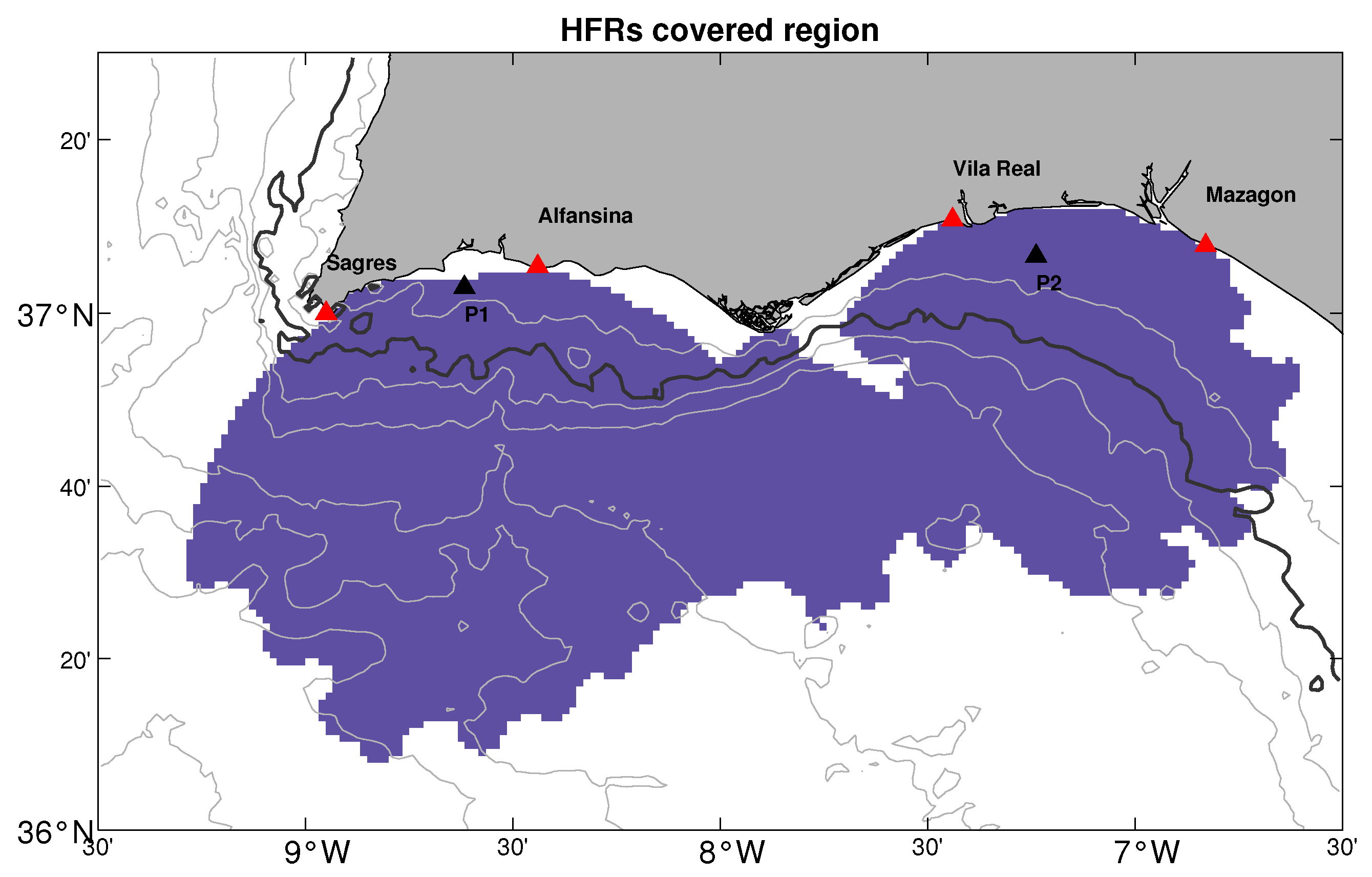
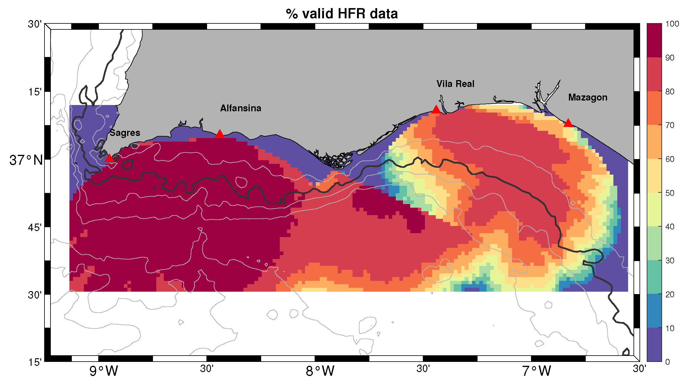
2.1. Data Collection

2.1.1. Current Velocity

High-Frequency Radars have been widely used as a powerful observing network for a wide range of application, such as coastal zone management, oil spill response, tsunami alert and validation of numerical models or satellite data (for a comprehensive review, see [53]). HFRs measurements are obtained by land-based sensors with high temporal resolution, increased spatial coverage and a low cost maintenance budget with respect to other sensors, both land- and satellite-based [54]. Thanks to the collaboration between the main Portuguese and Spanish oceanographic institutions, under the Trans-regional Radars for Environmental applications (TRADE) project coordinated by Puerto del Estado and supported by European FEDER funding, a shore-based Coastal Ocean Dynamic Application Radar (CODAR) SeaSonde System (13.5 MHz transmission) provides real-time hourly data on currents velocity detected from four sites of the southern Iberian coast (see the red triangles in Figure 3): Mazagón (37°7′N, 6°49′W), Vila Real de Santo António (37°10′N, 7°26′W), Alfanzinha (37°5′N, 8°26′W) and Sagres (36°59′N, 8°56′W). The first two started operating in 2013, covering the eastern part of the Gulf, while the third and the fourth ones were installed in 2014 and 2016, respectively, in order to extend the coverage to the entire region in front of the southern Iberian coast. The processing technique involves the use of direction-finding radars, which collect the phases and amplitudes of radio signals received by the four antennas placed along the coast. Even if the main goal of the project was to prevent the risks associated with navigation in the Strait of Gibraltar and along the southern coast of the Iberian Peninsula, many other applications took advantage of the information provided by these radars [55].

Covering a distance of about 75 km, ocean surface currents in the Gulf of Cadiz provided by the system and accessible via OpenDAP (http://opendap.puertos.es/thredds/catalog.html, accessed on 23 July 2021) were analyzed for the year 2017. The original dataset provides hourly near-real time surface ocean velocity over a regular grid at 1.5 km spatial resolution over a region that covers a wide part of the Gulf (the purple area in Figure 3). Before the data processing, a cut in the region was made to reduce the area of study from 9.1W to 6.6W in longitude and from 36.5N to 37.2N in latitude. This operation was carried out by means of the Climate Data Operators (https://code.mpimet.mpg.de/projects/cdo/, accessed on 23 July 2021) (CDO) options, which is a collection of command-line operators used to manipulate climate data in NetCDF format. For a preliminary idea of the continuity of the countercurrent between the eastern and the western part of the GoC, two significant locations were chosen for a preliminary analysis of the current velocity provided by the HFR system (indicated by black triangles in Figure 3): the first one is located at the point with coordinate (7°14′W, 37°6′N), which has been chosen due to some previous work carried out by the Applied Physics Department of the University of Cadiz (UCA) during the years 2013–2014 concerning the validation of the HFRs data with Acoustic Doppler Current Profiler (ACDP) data collection at that point [51,56]. The dataset derived from that sampling allowed us to validate the reliability of the data measured by the HFRs system in the Gulf of Cadiz. Moreover, it was located between the 50 m and 100 m bathymetry lines, where the CCCs have been widely observed in several previous works (e.g., [17,24,25,57]). The second location is at the point with coordinates (8°36′W, 37°3′N), which is situated in front of Algarve, the Portuguese side of the Iberian coast, in the middle of a region where the CCCs have been widely reported.

2.1.2. Meteorological Data

In order to evaluate the influence of remote atmospheric forces over the surface circulation in the Gulf of Cadiz, mean sea-level pressure and wind direction and intensity over the western Mediterranean have been analyzed.

Satellite-derived data have been obtained from the ERA5 (https://cds.climate.copernicus.eu, accessed on 6 September 2021) database distributed from the European Centre for Medium-Range Weather Forecast (ECMWF) through the Climate Data Store (CDS) provided by the Copernicus Climate Change Service (C3S). The ERA5 reanalysis covers the global climate and weather indicators for the past four to seven decades and the data considered in this work were selected from the ERA5 hourly data on single levels from 1959 to the present dataset [58] for the year 2017.

We analyzed the eastward and northward components of the 10 m wind provided by ERA5 over the Gulf of Cadiz (see the green box in Figure 2). These components included the horizontal speed of air moving towards the east and the north, respectively, at a height of ten meters above the surface of the Earth (in meters per second). The combination of these two components allowed us to evaluate the speed and direction of the horizontal 10 m wind over the selected region n from 35.5N to 37.7N in latitude and from 9.5W to 5.5W in longitude.

From the same dataset, we downloaded the MSLP field over the Ligurian Sea, which is the pressure (force per unit area) of the atmosphere at the surface of the Earth, adjusted to the height of mean sea level. This parameter is a measure of the weight that all the air in a column vertically above a point on the Earth’s surface would have, if the point were located at mean sea level. The hourly data are provided at 0.25° × 0.25° spatial resolution and were selected to cover the region from 42.7N to 44.6N in latitude and from 5.9E to 10.5E in longitude (see the red box in Figure 2).

2.1.3. Sea Surface Temperature

Daily gap-free (L4) sea surface temperature data at 0.01° × 0.01° spatial resolution were derived from the Mediterranean SST Analysis provided by the Copernicus Marine Service (https://marine.copernicus.eu/, accessed on 6 September 2021) (Product ID: SST_MED_SST_L4_NRT_ OBSERVATIONS_010_004_c_V2). The data provided are obtained from infrared measurements of daily (nighttime) merged multi-sensor estimation of the foundation SST collected by satellite radiometers. This value is defined as the temperature free, or nearly-free, value of any diurnal cycle, and SST fields are produced by selecting only the highest-quality values in order to reduce cloud contamination. Finally, to obtain a gap-free image, data are optimally interpolated by the provider over a regular grid, as detailed in [59]. The entire region covers the whole Mediterranean Sea and an eastern part of the Atlantic Ocean, which includes the Gulf of Cadiz. For this Ultra-High Resolution (UHR) L4 SST product, the validation analysis produced a mean bias of −0.078 ± 0.003 °C and a root mean squared deviation (RMSD) equal to 0.408 ± 0.003 °C [60].

2.1.4. Chlorophyll Distribution

The chlorophyll-a concentration is derived from biogeochemical daily and gap-free L4 products reprocessed for the North Atlantic area by the Copernicus Marine Service based on the ESA Climate Change Initiative (ESA-CCI) reflectance inputs (Product ID: OCEANCOLOUR_ATL_CHL_L4_REP_OBSERVATIONS_009_098, now changed to OCEANCOLOU R_ATL_BGC_L4_MY_009_118). This product is a multi-year (MY) time series produced from a consolidated and consistent input dataset covering the period from September 1997 to six months before the date of the full reprocessing, including a space–time interpolation algorithm at 1 km spatial resolution. For this product, the validation process shows a bias and an RMSD equal to 0.04 mg m⁻³ and 0.35 mg m⁻³, respectively [61].

2.2. Data Processing

A key feature for understanding oceanographic processes in time relies on the relationship between time series of different variables at nearby and remote locations. In order to carry out a direct comparison between different datasets and obtain equally significant statistics measures for every point of the considered area, we will process the current velocity fields obtained from the HFRs system through a set of operations. A method widely used in environmental applications to capture the variability at all time scale of the relation that links together various physical variables is through the Empirical Orthogonal Functions analysis (e.g., [62,63,64]), which is explained in detail in Section 2.2.1. The core of this method is based on the decomposition of a signal into a series of data-based orthogonal functions, with the property that only the first n of these functions (where n has to be determined in each case) are needed to optimally reconstruct the initial signal [65]. The main idea is to use the autovectors and eigenvalues of the covariance matrix, which statistically represents the relations between variables, to find the patterns responsible for the largest parts of the variance of our dataset [66]. Once the main functions are found, a low-pass filter and a temporal interpolation are applied to isolate the sub-inertial signal of the current and fill the gaps in the temporal series.

Finally, to analyze the connection between local and remote physical variables, a standard correlation analysis has been carried out, as detailed in Section 2.2.2.

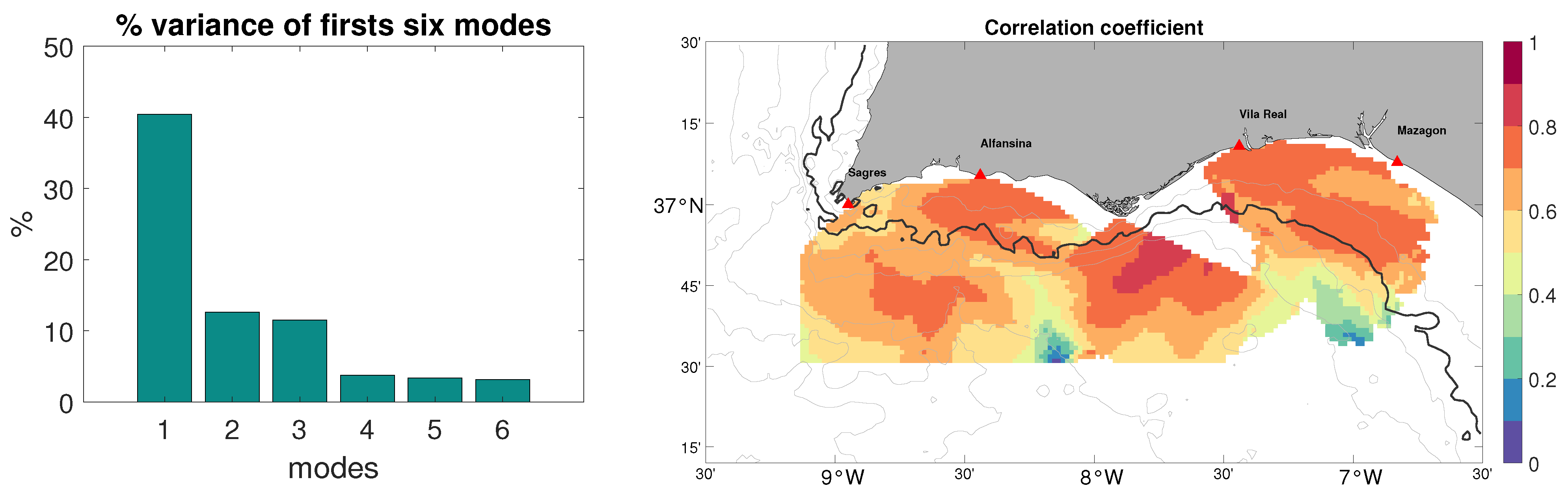
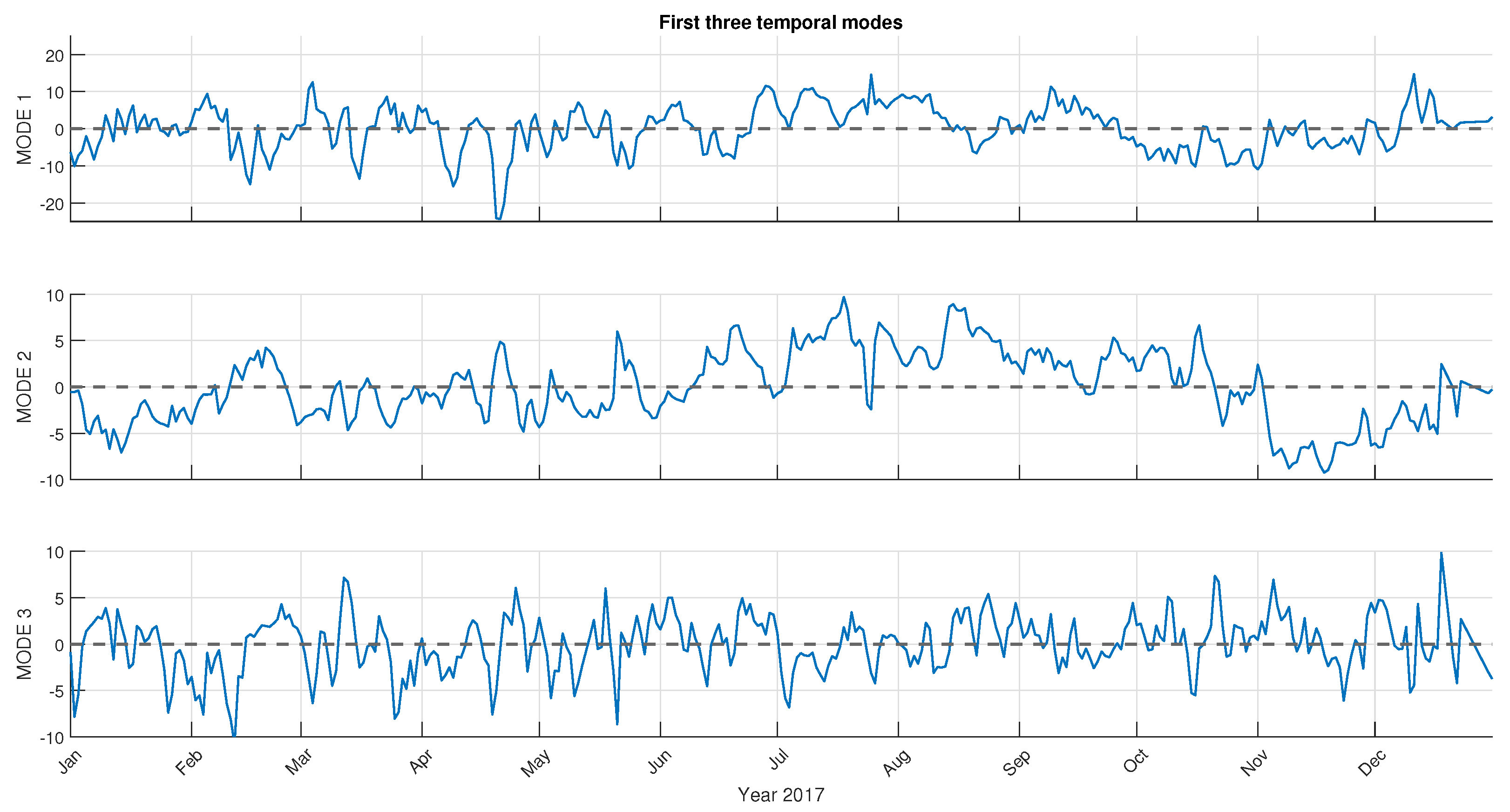
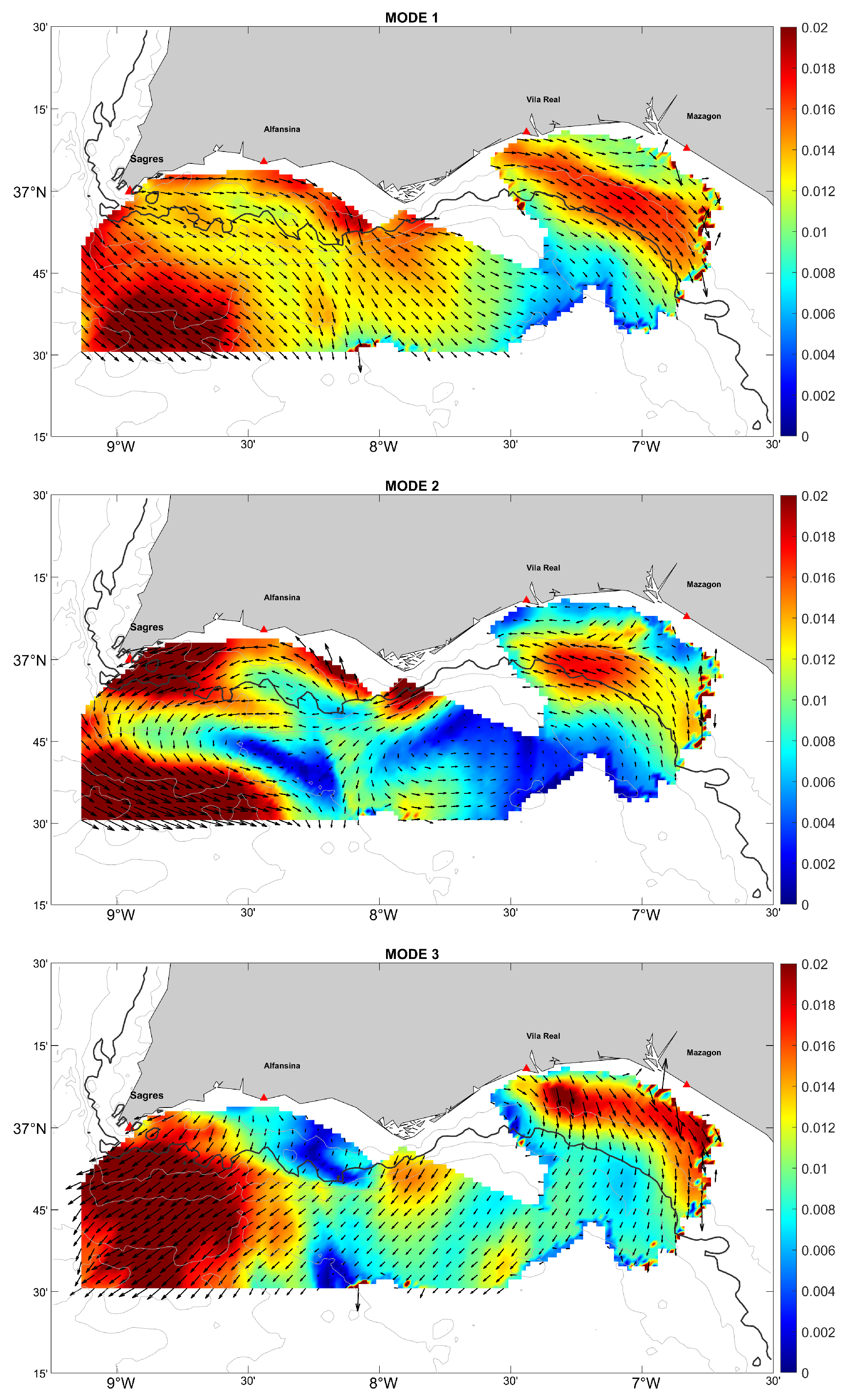
2.2.1. Empirical Orthogonal Functions

Let $\mathbf{S}$ be the data matrix whose columns represent the observation values and whose rows represent the time of the observation, i.e., $S_{i,j}=S(x_i,t_j)$ is equal to the data collected at the location $x_i$ at the time $t_j$. In our case, the columns of the data matrix $\mathbf{S}$ describe the time series at each grid point, whereas the rows the geographic distribution of the velocity fields at a particular time. Then, the Singular Value Decomposition (SVD) of our matrix is a factorization of the form

$$\mathbf{S}=\mathbf{U}\mathbf{D}{\mathbf{V}}^T,$$

(1)

where $\mathbf{D}$ is the diagonal matrix containing the (uniquely determined) singular values of $\mathbf{S}$, and $\mathbf{U}$ and $\mathbf{V}$ are real orthogonal matrices containing the right and the left singular vectors, respectively. Subtracting the temporal mean of each series from $\mathbf{S}$, we find that the data matrix has zero mean vector and, therefore, we can write the covariance matrix $\mathbf{C}$ as

$$\mathbf{C}=\frac{1}{N-1}\mathbf{S}{\mathbf{S}}^T,$$

(2)

where N is the number of observations for each grid point. Equation (2) implies that

$$\mathbf{C}=\frac{1}{N-1}\mathbf{U}\mathbf{D}{\mathbf{V}}^T\mathbf{V}\mathbf{D}{\mathbf{U}}^T=\frac{1}{N-1}\mathbf{U}{\mathbf{D}}^2{\mathbf{U}}^T,$$

(3)

by orthogonality of the matrix $\mathbf{V}$. Equation (3) tells us that the covariance matrix has the same left singular vectors as the data matrix and that each vector of the matrix $\mathbf{U}$ contributes to the total variance, an amount given by the diagonal element of ${\mathbf{D}}^2$. These modes of variations in $\mathbf{U}$ are called Empirical Orthogonal Functions. Moreover, since the total variance is also given by the sum of the squared singular values, we can divide them by the trace in order to obtain the percentage contribution $p_i$ of each mode $m_i$, i.e.,

$$p_i=\frac{m_i^2}{{\displaystyle \sum _{i=1}^n}{m}_i^2},$$

(4)

where n is the number of modes.

Although conventional EOFs can identify the dominant spatial patterns, the information on the different components of our variable evolution might be not fully detected. To capture this variation in cases that could be linked to the same physical process, the employment of the so-called real EOFs is required. Therefore, the same processing method described above is applied to a new data series of data ${\mathbf{S}}_C$ given by the combination of two components $\mathbf{X}$ and $\mathbf{Y}$, i.e.,

$${\mathbf{S}}_C=[\mathbf{X},\mathbf{Y}].$$

(5)

This method allows us to obtain a physically consistent analysis of the velocity fields due to the simultaneous processing of both the zonal and the meridional component.

In order to decide the number of modes needed to reconstruct the series, ref. [67] proposed to estimate the error produced by the EOFs approximation as

$$\Delta \lambda \approx \lambda {\left(\frac{2}{n}\right)}^{\frac{1}{2}},$$

(6)

where $\lambda$ is the eigenvalue of the covariance matrix and n is the number of statistically independent samples in the data. Then, a mode is considered significant only if the error defined in (6) is smaller than the distance between the corresponding neighboring eigenvalues. The numerical simulations have been carried out with a Matlab code.

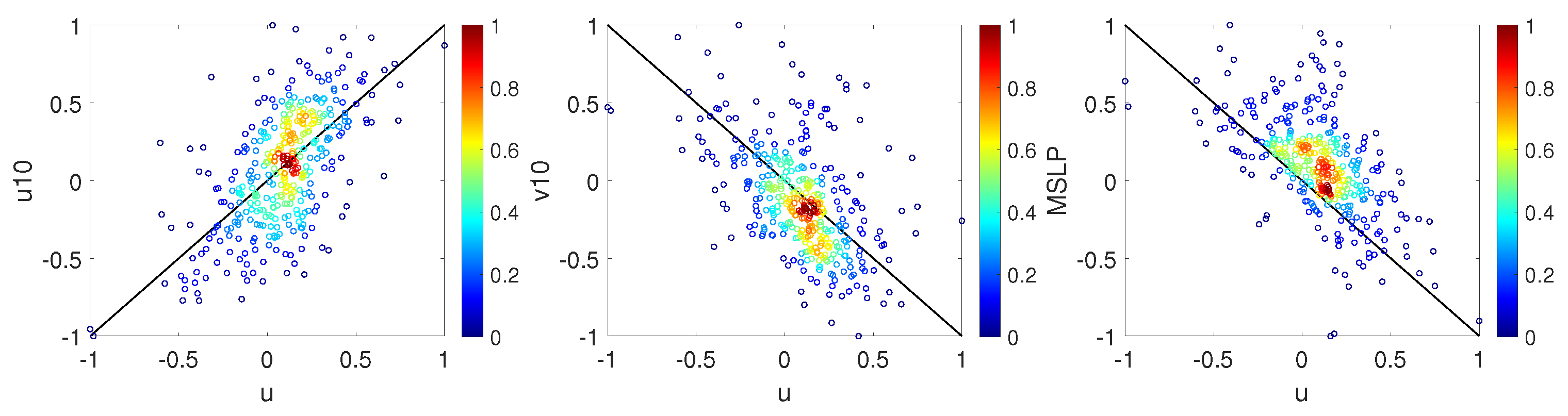
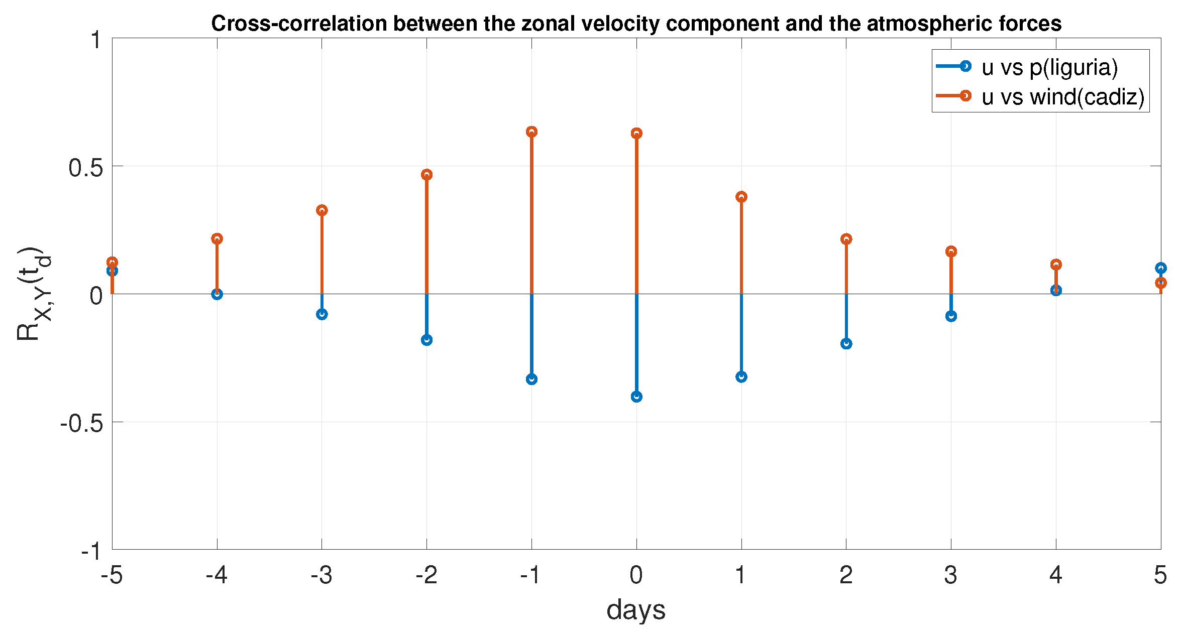
2.2.2. Correlation Analysis

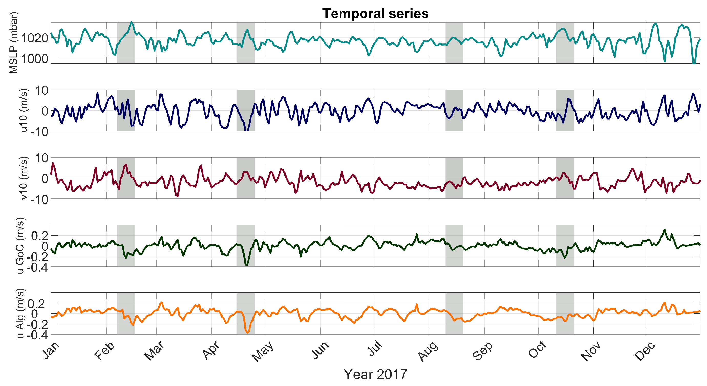
It has been widely established that there is a strong connection between many physical and biological environmental variables at short and large spatial and temporal scales. The datasets derived by remote-sensing instruments are sampling observations that evolve over space and time and, therefore, are perfectly suited for classical and advanced statistical correlation analysis. These techniques allow us to measure the strength of the relationship between two variables, namely the level of change in one variable due to the change in the other. Several techniques were developed to explore the relation among different geographical locations or to identify unknown relations among variables.

In this study, we carried out a classical correlation analysis between the main physical variables (namely the two components of the current velocity and the main meteorological forces). Firstly, all variables were scaled through a standard min–max normalization, following the rule:

$$x^{\prime }=a+\frac{(x-min(x))(b-a)}{max(x)-min(x)},$$

(7)

where $[a,b]=[-1,1]$. Therefore, there was a positive (negative) correlation between two variables when an increase in one variable led to an increase (decrease) in the other. This correlation was measured through the calculation of the correlation coefficient, which provides the intensity of the relation between two variables X and Y and is defined as

$$R(X,Y)=\frac{1}{N-1}\sum _{i=1}^N\left(\frac{X_i-{\mu }_X}{{\sigma }_X}\right)\left(\frac{Y_i-{\mu }_Y}{{\sigma }_Y}\right),$$

(8)

where N is the observation number, ${\mu }_X$ and ${\sigma }_X$ are the mean and standard deviation of X, respectively, and ${\mu }_Y$ and ${\sigma }_Y$ are the mean and standard deviation of Y, respectively.

Furthermore, a cross-correlation analysis was made between the same temporal series in order to measure the similarity between a discrete-time sequence and shifted/lagged copies of another sequence as a function of the lag. This analysis allows us to capture the changes in a variable X due to the variability of Y with a certain time delay $t_d$ as

$$R_{X,Y}(t_d)=E\left[X_{i+t_d}{Y}_i^{\ast }\right]=E\left[X_{t_d}{Y}_{i-t_d}^{\ast }\right],$$

(9)

where E represents the expected value operator and the asterisk denotes complex conjugation.

2.3. Data Analysis

The original dataset derived from the HFRs system in the Gulf of Cadiz presented in Section 2.1.1 and providing hourly near-real-time surface ocean velocity for the year 2017 presents several missing data. As detailed in

Table 2. Number of (hourly) missing data in the HFRs dataset for the year 2017 listed by month.

	Jan	Feb	Mar	Apr	May	Jun	Jul	Aug	Sept	Oct	Nov	Dec
number of missing data	25	1	104	8	0	0	71	30	8	26	16	315

, for the year 2017, there are 8147 hourly data (which means 613 missing data), which mostly occurs due to malfunctions of the instruments or to other external factors, such as radio frequency interferences, antenna pattern, distortions, environmental noise, etc. [27].

In order to ensure a significant analysis, we considered a reduced area, selecting only the grid points with more than 70% of available data in the temporal series (see Figure 4). Among those, the remaining missing values were set equal to the temporal mean of the location, obtaining a gap-free dataset and preserving the zero mean property of the matrix, as required from the EOFs algorithm. Since the physical processes that prevail in the various parts of the GoC can be very different, to obtain a realistic reconstruction of the missing values, we divided our area of study in three subregions that we can identify with the eastern part of the Gulf, a central intermediate region in front of Cape Santa Maria and the western part of the GoC covering the marine area off the Portuguese coast.

Therefore, for each velocity component (separately), we applied the conventional EOFs algorithm and the missing data were replaced by the reconstructed time series truncated at the first mode. A low-pass Fast Fourier Transform (FFT) filter with a cutting period of 30 h was applied to the velocity time series in order to remove the tidal signal and isolate the contribution of the low-frequency processes mainly caused by atmospheric forcing [33,68]. The daily mean was then calculated and the missing days were linearly interpolated to cover the whole time series for the year 2017. Finally, real EOFs analysis was applied to both components of the velocity fields in order to identify the spatial and temporal patterns in our dataset. The original series was then fully reconstructed with the first three modes of the EOFs, which were found to be the significant ones according to the criteria defined in Equation (6).

3. Results and Discussion

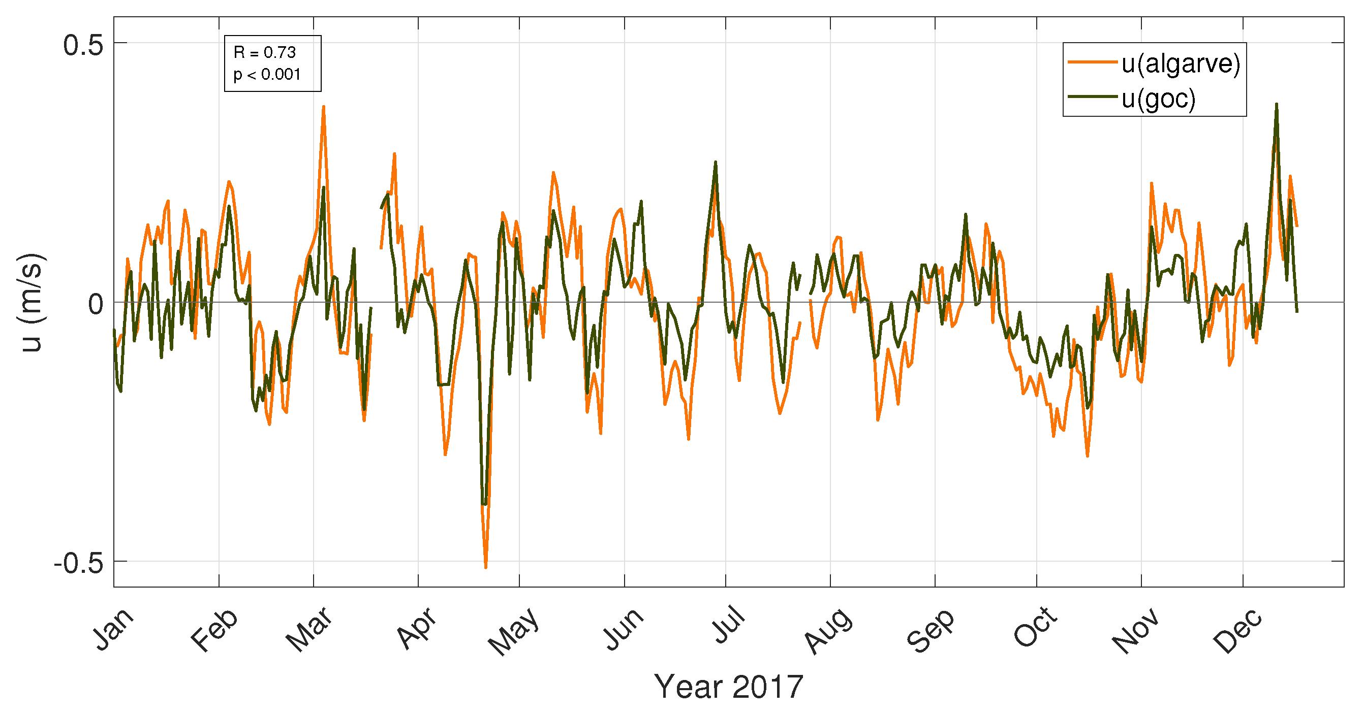
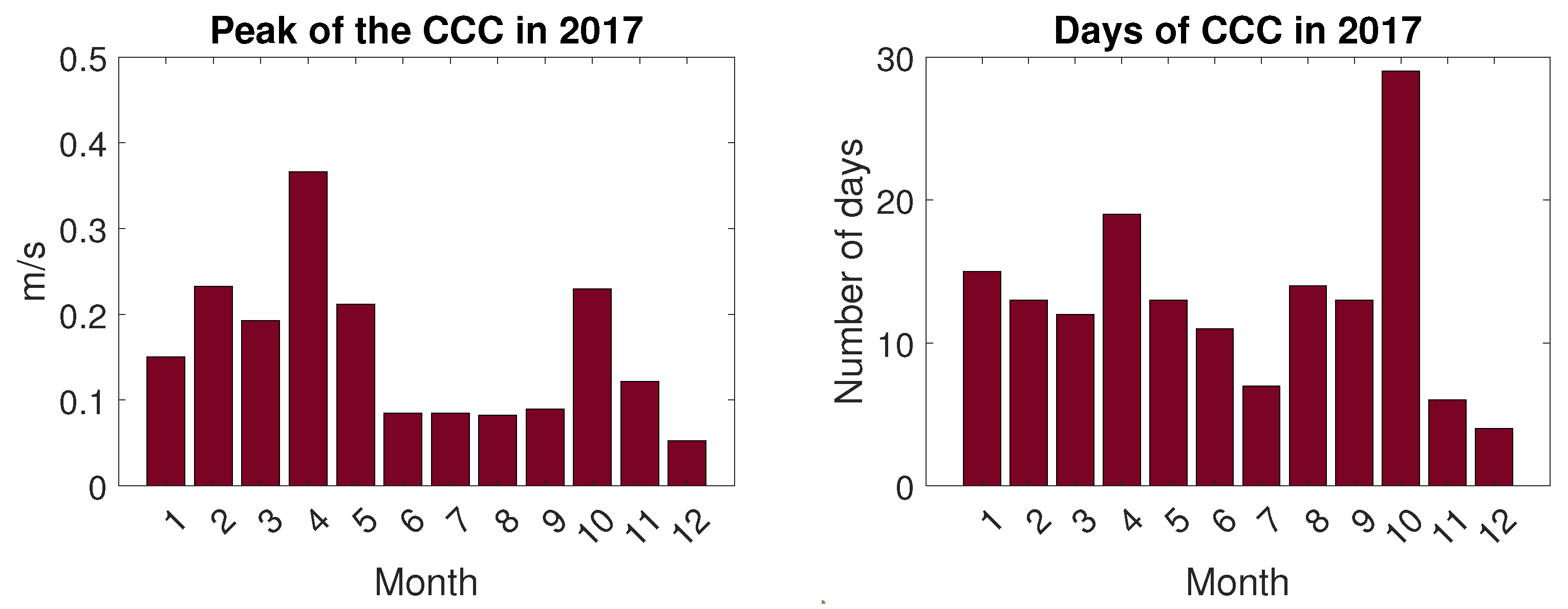
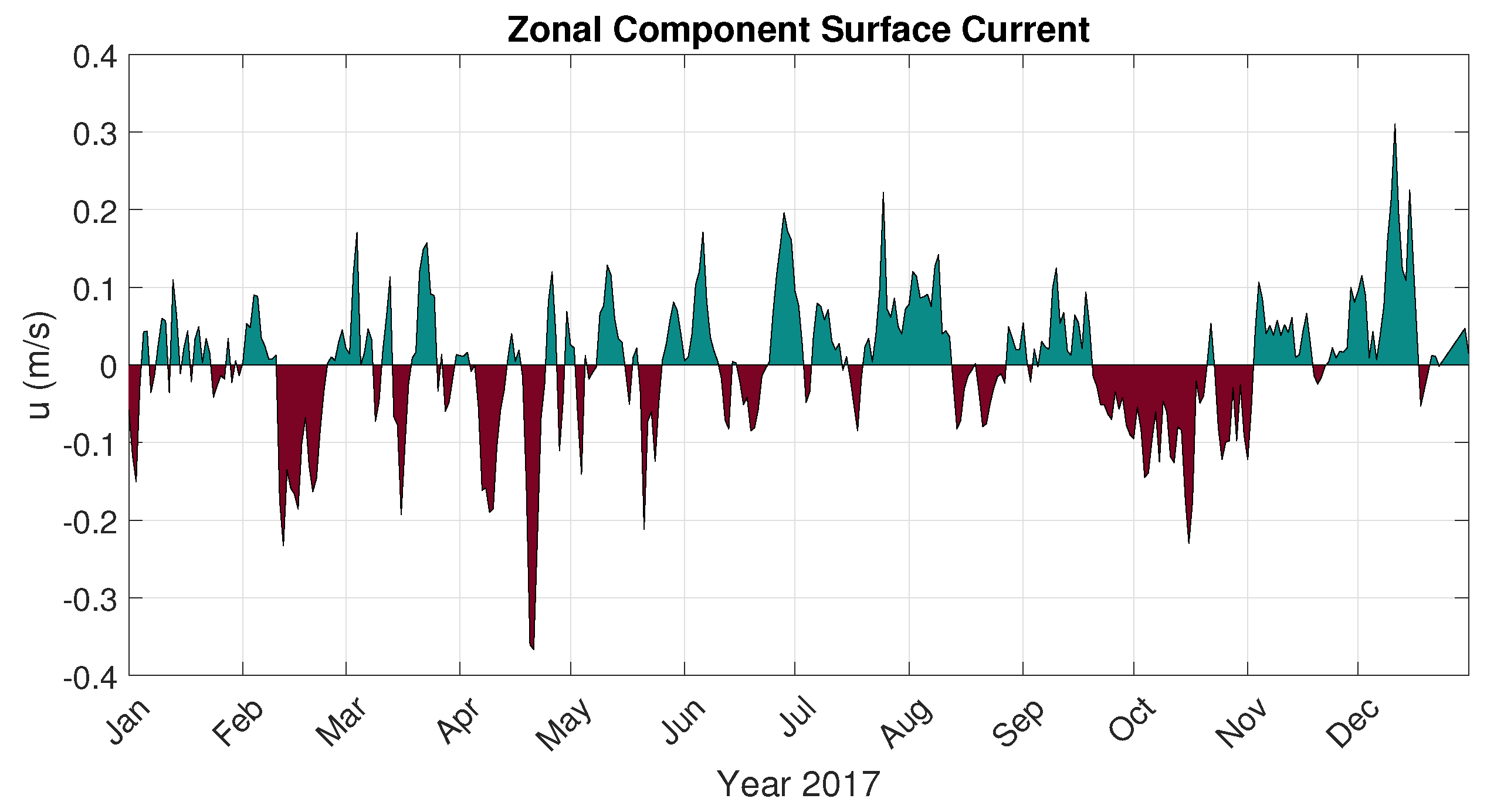
3.1. Surface Current Analysis

Since our aim was to inquire if there is a certain continuity of the countercurrent between the different parts of the Gulf, we compared the evolution of the zonal component of the current velocity during the year 2017 at two different but significant locations (see the black triangles in Figure 3). The first temporal series (presented in green in Figure 5) corresponds to the u component of the current velocity measured by the coastal radar system at the point with coordinate (7°14′W, 37°6′N), while the second location, whose corresponding temporal series is represented in orange, is placed at the point with coordinates (8°36′W, 37°3′N). The temporal series shown in Figure 5 are the result of the processing described in Section 2.3 without applying the final real EOF analysis, which resulted in a daily mean gap-free current velocity evolution at the extracted locations after a low-pass filter was applied (with a cutting period of 30 h). It is quite apparent that there was a correlation between the two temporal series (with a Pearson correlation coefficient equal to 0.73), showing the continuity of the coastal dynamics in the GoC.

In Figure 6, we can observe a general characterization of the intensity and duration of the CCCs events during 2017. Even though it is clear that the meteorological drivers play a crucial role in their development and growth, a clear seasonality has not been found. Despite the conclusion drawn in [69], according to which there is an alternating behavior of the circulation over the continental shelf, where a predominantly eastward flow is found during winter and spring while the CCCs develop mainly from July to October, we found that the alongshore westward flow can be observed throughout the year, in agreement with more recent works on the topic [24,51,70]. In fact, CCCs occurred on 156 days (i.e., 42% of the year) in 2017 (Figure 6, right panel). The more intense event occurred in April, followed by February and October, while during the summer, the westward zonal velocity remained below the 0.1 m/s (Figure 6, left panel). Although the stronger events occurred in April and in February, with 15 and 13 days of CCCs, respectively, it is worth to noting that in October 2017, there were 29 days of westward flow, which was the highest value recorded for the whole year (Figure 6, right panel).

Motivated by this result, our goal is to explore, by means of the EOF analysis, the temporal and spatial distribution patterns of the current velocity field related to the sub-inertial signal (especially for the zonal component), in order to characterize the intensity and the main driving forces of the CCCs along the whole southern Iberian peninsula.

The main results of the analysis performed on the daily mean surface current velocity in the Gulf of Cadiz for the year 2017 are presented in Figure 7, Figure 8 and Figure 9. As explained in Section 2.2.1, the goal of this technique is to decompose the spatial and temporal variations of a given variable into spatial distribution patterns through a relatively small number of variables that contain as much information as possible from the original dataset. The idea is to group the signals that present a common behavior in their variation of time in a set of empirical orthogonal functions whose percent variance defines how much they contribute to the original data.

In Figure 7, the percentage distribution of the variance explained by the first six modes derived from the EOF analysis for the surface current velocity is presented on the left panel. The first mode explains 40%, while the second and the third ones explain approximately 13% and 11% of the variance, respectively. In the right panel of the figure, we can observe the correlation coefficient map between the current velocity measured by the HFR system and the mode one-based synthesis originating from the real EOF analysis, demonstrating the ability of this technique to capture the most energetic signals of the current. Due to the small percentage of the rest of the modes, according to the criteria defined in Equation (6), we will consider the first three modes as the main representatives for our series, jointly explaining 64% of the total variance.

In Figure 8 and Figure 9, the temporal weights and spatial weight maps of the first three EOFs modes are shown, respectively. The first three temporal weights indicate the main time variability features, while the spatial weights indicate where a given EOF mode is more or less intense. We can observe from these results that the first mode seems to contain the expression of the CCCs. In fact, the direction of the current can be deduced from the multiplication sign between the temporal modes and the spatial coefficients. In Figure 9, we observe that the spatial coefficients associated with the first mode show the main direction of the flow with a certain intensity and, to obtain the temporal variation of the surface velocity, they have to be analyzed in combination with the correspondent temporal mode. This means that the negative values in the temporal amplitude in Figure 8 represent the tendency of the current to flow westward, while the positive values describe the eastward flow. The time series of the first temporal mode shows that it reaches its minimum in April, with low values in February and persistent negative values in October. The second temporal series presents mostly negative values in the first half and during the last two months of the year, while it almost exclusively positive values from June to October. The third temporal mode, however, presents an alternative behavior without defining a very clear pattern. The result of the EOF analysis confirms the connection between the subregions, as already noticed in Figure 5. In fact, the amplitude represented by the spatial coefficients for the first mode shows a clear tongue of intense alongshore current between the 50 m and 100 m bathymetry lines (Figure 9). The second mode presents a clear intensity division between positive and negative values in the northern and southern parts of the Gulf, respectively, while the third mode describes a similar separation between the oriental and the occidental parts. To focus on the alongshore flow, from now on, only the zonal component of the current will be analyzed.

In Figure 10, the temporal series of the zonal component of the current velocity derived from the HFRs data processing at the point with coordinate (7°14′W, 37°6′N) for the year 2017 is shown, and corresponds to the location of the ACDP already analyzed in [51,56]. The green-shaded positive values represents the eastward flow, while the red-shaded negative values represent the CCCs. Figure 10 confirms the relation between the first mode temporal coefficients derived by the EOF analysis and the CCC events. In fact, the higher values of the temporal coefficients for the first mode correspond to the higher values for the horizontal component of the current velocity recorded by the radars. The series of the u component presents alternative changes in the direction of the flow, without any clear trend in favor of eastward or westward flows. The zonal velocity reaches its minimum (namely its strongest intensity) equal to −0.38 m/s on April 20, exactly the same day on which the first temporal mode reaches its minimum in the EOFs analysis. Analogously, we can observe high negative values in February and a persistent westward flow in August and October. However, there is no clear pattern of the seasonality of these events, considering that the more intense CCCs are detected in winter and spring, while the most persistent ones occur in autumn. Even if there is clear evidence of a predominant eastward flow in November and December, and from late May to the start of August, the rest of the year is characterized by an alternation in the flow direction with a slight predominance of the CCC events in February and March and a clear predominance of westward flow in October.

Figure 11 shows a comparison between the same temporal series of the zonal current velocity (the black and orange lines at the bottom) and the two main atmospheric forces responsible for this kind of event. This comparison was based on the ERA5 dataset, namely the mean pressure sea-level over the Ligurian Sea (the first green line) and the u and v components of the wind at 10 m from the sea surface over the Gulf of Cadiz (the second blue line and the third red line, respectively) in 2017. The gray-shaded intervals represents the days of the strongest or more persistent CCCs events during the year, as highlighted previously. We can observe that there is a strict correlation between the highest values of the MSLP series and the lowest values of the zonal component of the current velocity. The highest value of the MSLP (equal to 1034.6 mbar) was found on February 15, which is in correspondence with the second strongest CCC event in the GoC. If we look at the entire series, during the three strongest events of westward flow in the Gulf of Cadiz, we can find a considerable high values of the mean pressure variation over the Ligurian Sea, which is in agreement with recent works that associate subinertial flow fluctuations in the Strait of Gibraltar with MSLP fluctuation in the Western Mediterranean Sea [33]. On the other hand, the wind velocity presents an alternative behavior with respect to the main CCC event during 2017. The zonal component varies along the whole year with high negative values (i.e., wind proceeding from east) from February to May, where the more intense event corresponding to 8.5 m/s is found on April 20, exactly like the strongest CCC event of the year. This event is characterized by the combination of a very high MSLP fluctuation over the Ligurian Sea with an intense wind blowing from the south-east, which is responsible for the accumulation of water masses near the coast and their movement toward the west. In summer and autumn, prevalent positive values are presented, describing a wind proceeding from west. The meridional component presents less intense variations, achieving a maximum value equal to 7.13 m/s during the CCC event in February, corresponding to the wind blowing northward. Excluding the CCC event in August (among the four highlighted with the gray-shaded zones), the other three occur under a wind proceeding from the south. Obviously, the easterlies contribute to the increase in terms of strength and intensity of the CCC, but an easterly wind is not a required condition for the westward flow to develop, as argued for example in [23,26].

The statistical analysis will clarify the relationship between different variables at nearby and remote location during a certain period of time. In order to capture the variability of the current as function of the main atmospheric forces, the correlation coefficients between these four variables are listed in

Table 3. Correlation coefficients and correspondent p-values between the u component of the current velocity derived from the EOF analysis of the HFR system in the GoC, the first mode and the main atmospheric forces considered in this study, namely the zonal ($u10$) and meridional ($v10$) component of the wind over the GoC and the MSLP over the Ligurian Sea).

Correlation	$\mathit{u}\mathbf{10}$ (GoC)	$\mathit{v}\mathbf{10}$ (GoC)	MLSP (Lig)
u	R = 0.6	R = −0.49	R = −0.56
	$\left(p<0.001\right)$	$\left(p<0.001\right)$	$\left(p<0.001\right)$
Mode 1	R = 0.74	R = −0.51	R = −0.52
	$\left(p<0.001\right)$	$\left(p<0.001\right)$	$\left(p<0.001\right)$

. In the first row, it quickly becomes clear how the local wind (in particularly the horizontal component) and the fluctuation of the pressure over the sea surface in the Western Mediterranean influence the zonal component of the flow. The negative coefficient equal to −0.56 describes a correlation between the decreasing of u values (namely the flow toward a western direction) arising out of the increase in the MSLP over the Ligurian Sea, and is also shown by the density scatter plots of Figure 12. Analogously, we can infer a very strict connection between the westward flow and the wind blowing from the east, presenting a correlation coefficient equal to 0.6. As we already observed, the first mode is the one more connected with the atmospheric forces contributing to the sub-inertial flow fluctuations in the area. In fact, the correlation (with R = 0.74) between the temporal series of the first mode and the horizontal component of the wind confirm this strong relation, as do the correlation coefficients associated with $v10$ and the MSLP over the Ligurian Sea (equal to R = −0.51 and R = −0.52, respectively).

It is important to take into account that most of the the relevant environmental processes often occur with a (variable) time lag with respect to the factors that contributed to generating those events. For this reason it can be helpful to approach the temporal series through a more advanced statistical technique such as the cross-correlation analysis, which measures how related are two variables not only simultaneously but also with different time shifting. Figure 13 shows the cross-correlation between the u component of the surface current and the two main local and remote atmospheric forces, namely the MSLP in the Ligurian Sea in blue and the velocity of the wind at 10 m in the Gulf of Cadiz in red. It is clear not only that there is a relation between these variables, but that the result is not always instantaneous and could be caused by the events of the previous day. In particular, we can observe that the wind blowing from the east shows higher cross-correlation coefficient ($R_{X,Y}(t_d)=0.63$ with $t_d=-1$) with the westward flow of the current of the next day.

The countercurrent events analysis performed to date confirm the complexity of identifying the main physical forces driving these processes. However, without any doubt, the highest intensity of the countercurrent is always detected between the 50 m and 100 m bathymetry lines, inducing the accumulation of offshore waters near the coast. In order to characterize the consequences of these events, in the next section, we will analyze four selected case studies of CCCs that occurred in 2017, exploiting satellite-derived Chl-a and SST data as tracers for the surface circulation in the area.

3.2. Case Studies

In the present section, we analyze four case studies of CCC events that occurred in 2017 (highlighted by the gray-shaded boxes in Figure 11) through the comparison of surface current velocity measured by the HFRs system with chlorophyll-a distribution and sea surface temperature patterns derived from Copernicus L4 products.

The four events took place on 12 February, 20 April, 14 August and 16 October 2017. We represent the velocity fields together with the flow direction during the day where the current reaches its maximum values and the three adjacent days (namely, the day before and the two days after the main event). Therefore, the Chl-a (mg/m³) and the SST (°C) images are shown in a significant time range around those dates to evaluate the spatial variations of those variables due to the westward flow in the Gulf of Cadiz. The images were selected in order to capture the extension of the westward flow and the analyzed oceanographic features distribution resulting from the hydrodynamic forcing.

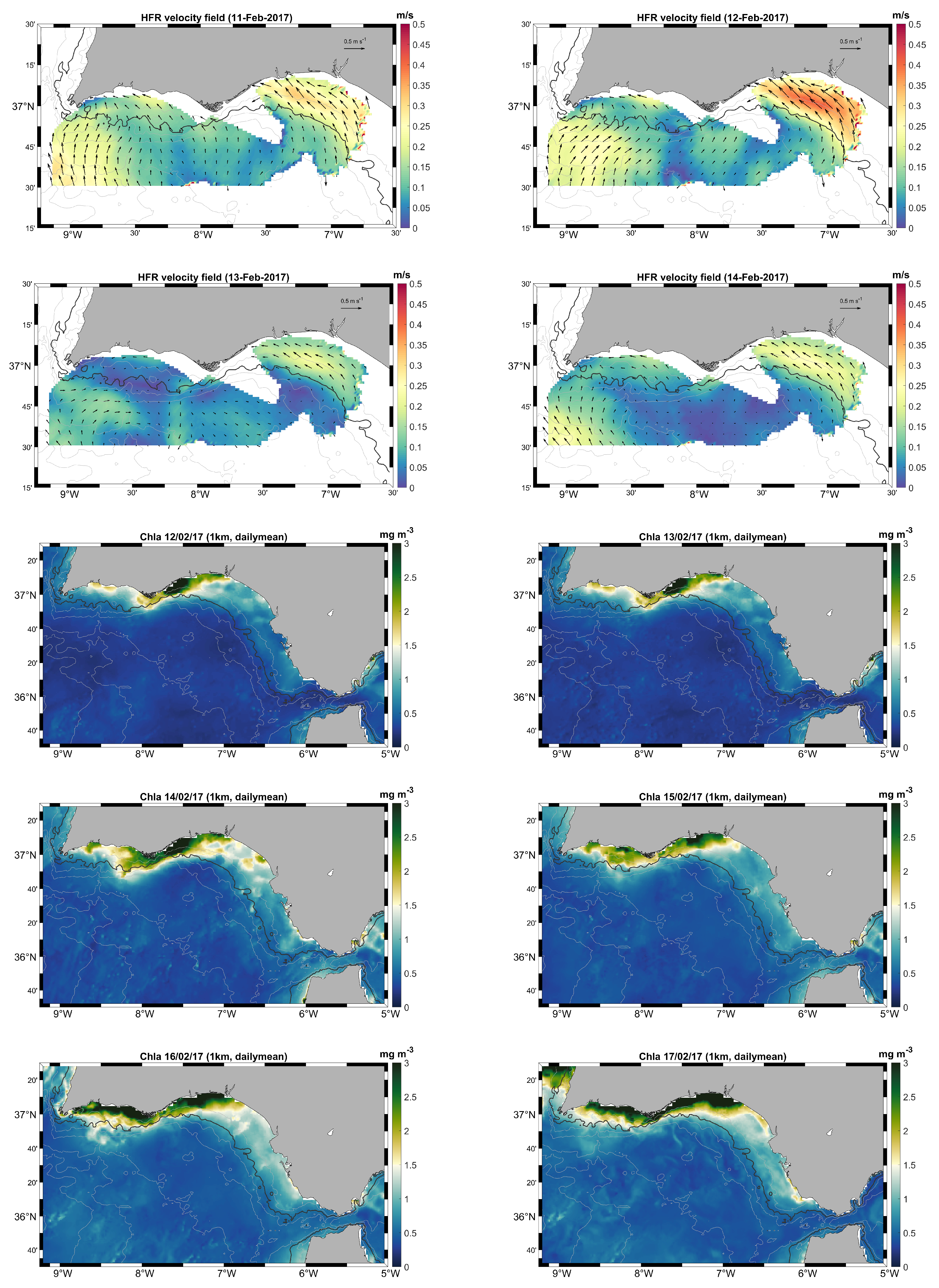
3.2.1. Case Study 1: February 2017

In Figure 14, the daily mean velocity field and the direction of the current from 11 February to 14 February 2017 are shown on the top four panels. During this CCC event, a persistent wind blowing from south-west is observed, which should hamper the development of the westward flow of the current (Figure 11). However, during the same days, the strongest fluctuation of the year for the mean sea-level pressure over the North-Western Mediterranean Sea is able to generate the variation in the subinertial current intensity, which results in a reduction in the intensity of the Atlantic inflow [33,36,71]. In these conditions, a great amount of water masses accumulate near the meridional Iberian coast with the help of the northward direction of the wind. The variation in the sea level finally enables the spread of the APG needed for the generation of the CCC. In fact, near the coast, we can observe an intense alongshore westward flow confined before the 100 m bathymetry line in the oriental part of the Gulf (with respect to Cape Santa Maria). This event was the second strongest CCC in the 2017, reaching maximum strength on 12 February, in proximity of the 50 m bathymetry line in the zone between the Tinto–Odiel–Piedras and Guadiana mouths. However, given the lack of available HFR data in the region that separates the eastern and the western part of the Gulf of Cadiz, it is difficult to understand the connection of the flow between the two sub-basins. In particular, we cannot appreciate if the alongshore westward current coming from the eastern part of the Gulf extends throughout the southern coast of the Iberian peninsula or if there are two separated coastal currents which remain in the sub-basins where they develop. In order to overcome this lack of information, we make use of other physical and biological features derived from satellite observations, which allow us to obtain (spatially) continuous information for the whole basin. In the L4 daily mean chlorophyll distribution for the days between 12 February and 17 February, it is clear that the nutrient-rich waters near the Tinto–Odiel–Piedras mouth are displaced toward the west, with a clear advection of the biological material beyond Cape Santa Maria, expanding the maxima of chlorophyll along the whole southern Iberian coast. From this sequence of images, we can infer that the coastal countercurrent is able to expand from the eastern to the western part of the Gulf (even if it loses strength), transporting the biological material up to Cape San Vicente.

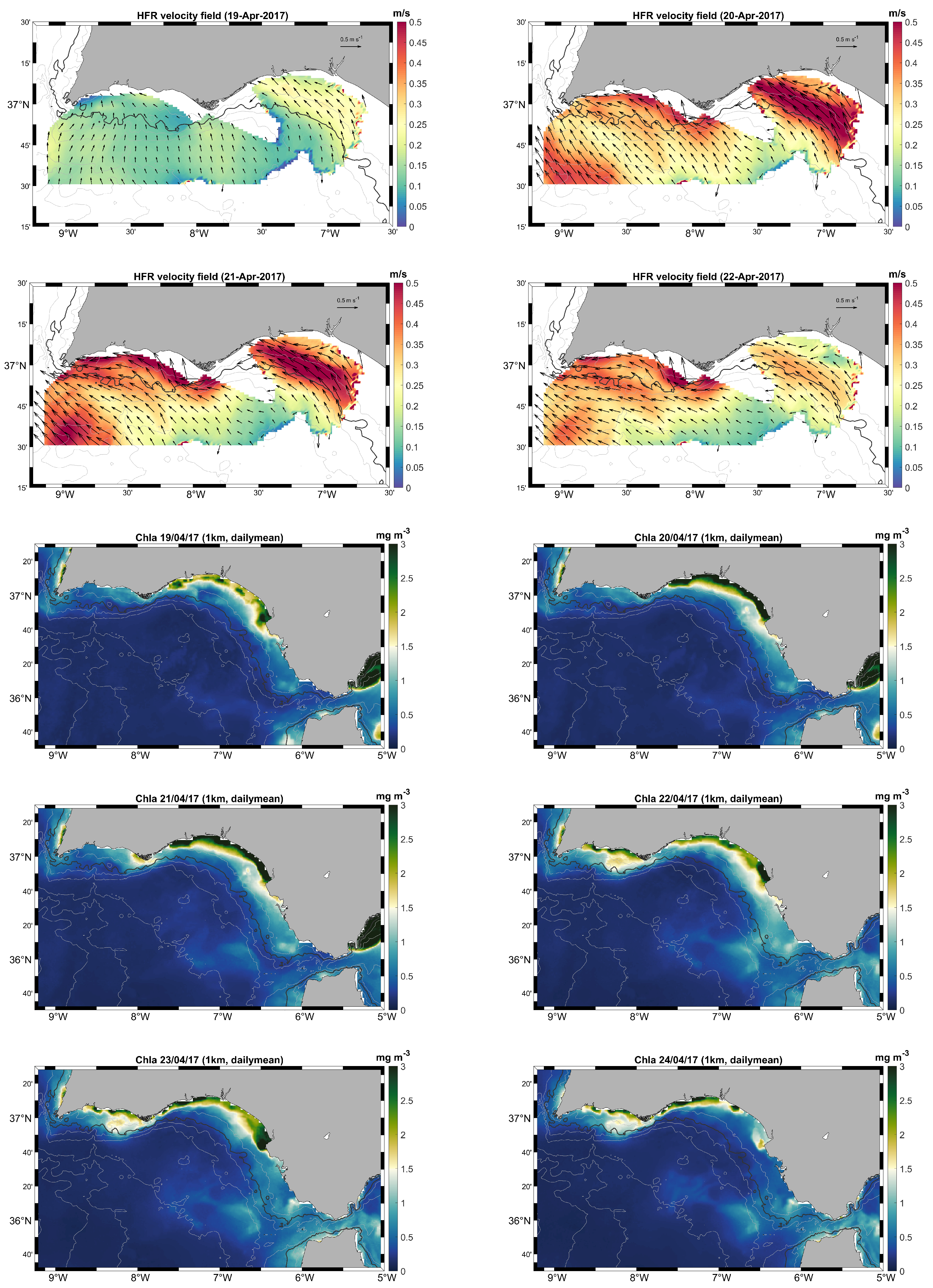
3.2.2. Case Study 2: April 2017

The CCC event that occurred between 19 and the 22 April 2017 is shown by means of the velocity field reconstructed from the HFRs data in the four top panels in Figure 15. This event is the strongest of the year, reaching a maximum velocity of over 0.4 m/s in the western part of the Gulf on 20 April, and continuing the day after in the eastern sub-basin. We already observed in Figure 11 that the coastal countercurrent that occurred on those days presented a clear correlation with the main atmospheric forcing: the atmospheric pressure over the Ligurian Sea presents one of the strongest fluctuations of the year, while local zonal winds are intensively blowing from the east during several days. This relation is also supported by the very high value of the temporal coefficients of the first mode during those days presented in Figure 7, which we know are more connected to the atmospheric processes [14,57]. The combination of these two particularly strong physical forces allows the development of the most intense westward alongshore current of the year. Even if we are still limited by the lack of HFR data in the proximity of Cape Santa Maria, the strength of the westward flow, which here firstly appears in the western part of the Gulf but clearly originates in the near Strait of Gibraltar, according to the results obtained by [33,51], suggests that the current may reach the Portuguese coast. The extension of this event, in fact, is clearly visible in the chlorophyll distribution (presented in the last six panels of the figure) in both the eastern and the western part of the basin. The CCC, once again being at its maxima between the 50 m and the 100 m bathymetry lines, accumulates nutrient-rich waters and then distributes them along the southern coast. In this case, the variation in the MSLP observed in the Western Mediterranean coinciding with local southerlies wind induces the accumulation of water masses against the coast and generate a geostrophic adjustment of the pressure gradients (transversal with respect to the coast) and create the conditions for the development of the coastal countercurrent.

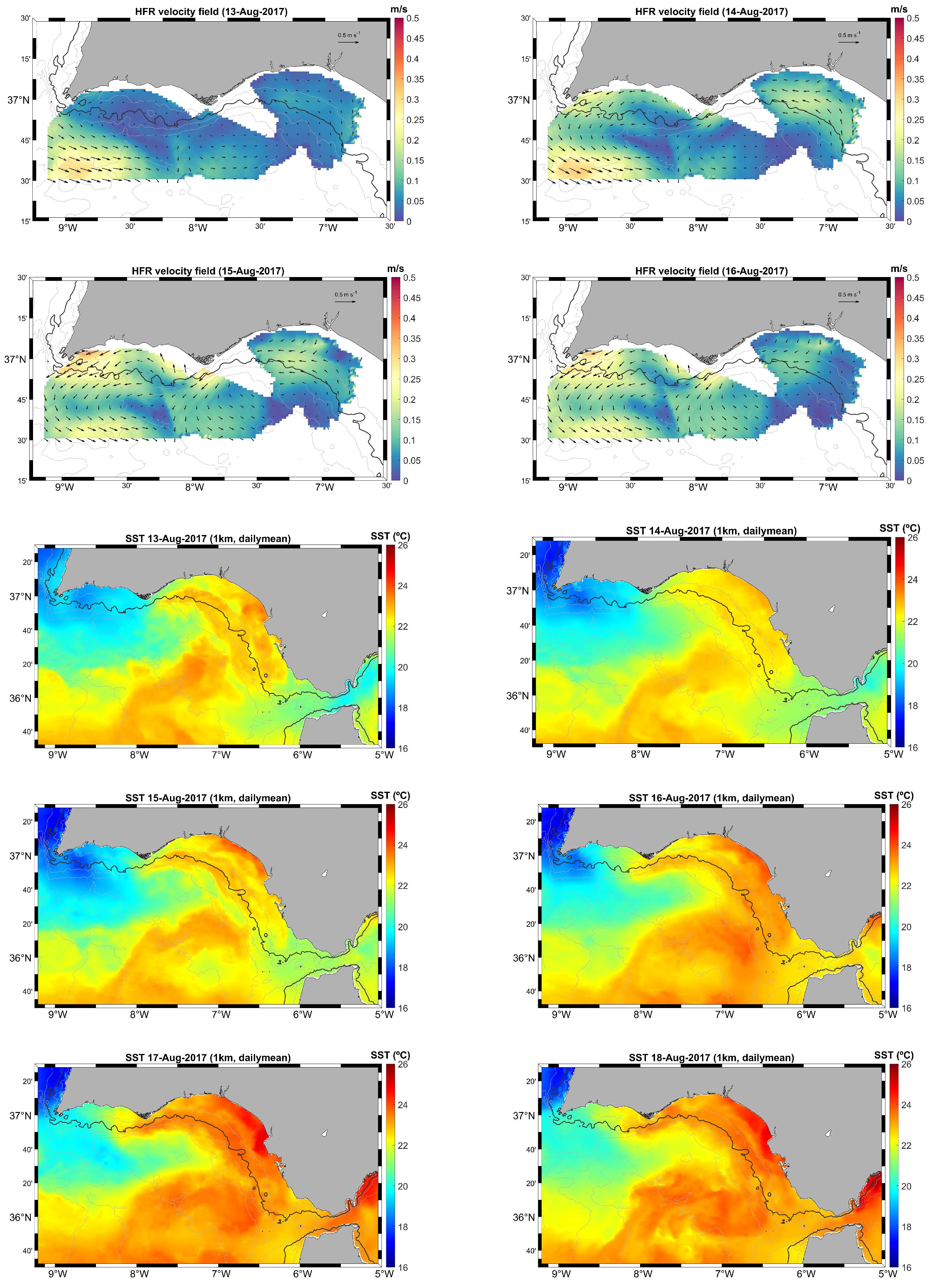
3.2.3. Case Study 3: August 2017

In the data for August 2017, we observe the development of a westward coastal current that lasts 8 days, starting on the 13th and reaching a maximum value lower than 0.2 m/s on 14 August. The velocity field for the first four days of this event (in the top four panels) and the sea surface temperature values from 13 August to 18 August (in the last six panels) are presented in Figure 16. As we already observed, while at large scales, SST responds to the interaction between air and sea fluxes and deeper waters mixing with the upper layers, if we consider meso and sub-mesoscale dynamics, SST distribution is mainly driven by horizontal advection. Even if the daily mean current velocity provided by the HFR data analysis seems to reveal two separate cyclonic cells over the platform, the SST images clearly show the classical warm tongue of waters, as observed in several previous works [30,43,72]. Although the intensity of this CCC is reduced with respect to the ones in February and April, a clear warm flow following the pattern delimited from the 50 m and the 100 m bathymetry lines expands from Cape Caraminal up to the western part of the continental shelf, as shown by the daily mean SST distribution images. During the first few days, the easterlies are blowing in a persistent northward direction in the $v10$ component, while the MSLP over the Ligurian Sea is slowly increasing (Figure 11). The warm countercurrent seems to be formed in eastern part of the Gulf, where the warm water accumulates against the eastern coast near the Strait of Gibraltar, progresses and recirculates cyclonically along the southern coast of the Iberian peninsula. The westward flow is then augmented or diminished by wind forcing. In particular, the quasi-permanent cyclonic circulation in front of the Portuguese coast of the GoC is clearly visible in HFR data patterns. The consequences of the eastward flow of this eddy can also be observed in the sea surface temperature images, where cold waters originating from the vertical western coast of Portugal are advected eastward from the main circulation beyond Cape San Vicente, where the cold filament develops, and accentuate the front with the warm CCC.

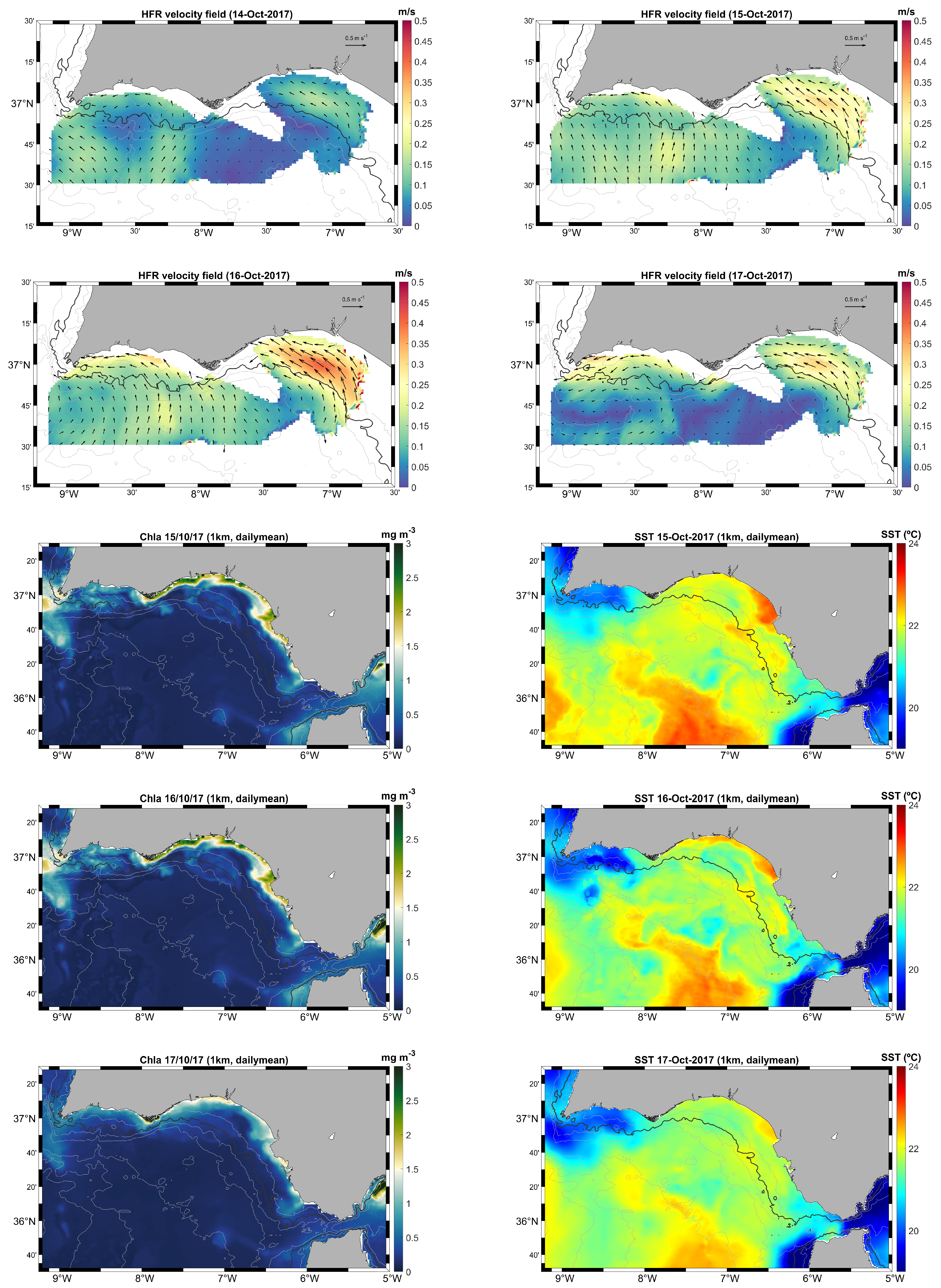
3.2.4. Case Study 4: October 2017

The first four panels of Figure 17 show daily mean current velocity (m/s) provided by HFR system from 14 October to 17 October 2017, where the CCC reaches its maximum values on the 16th. As mentioned before, this month is characterized by a persistent CCC with 26 days of westward flow, and is the longest event of the whole year. Analogously to the event that occurred in February, we can observe the surface circulation being driven by the southerly wind for the first two days and accumulating waters against the coast. However, in this case, the cyclonic eddy in the western part of the Gulf become clear on 17 October, separating the flow in two parts with respect to CSM, as extensively reported by [43]. Around the days on which the intensity of the countercurrent is higher, we can observe in the chlorophyll-a distribution (presented from 15 October to 17 October in the last three panels on the left of the figure) the tendency of this indicator to be displaced toward west (especially in proximity of the plume generated from Cadiz Bay and the Guadalquivir mouth), reaching the western side of Cape Santa Maria but without going further. The maxima of chlorophyll remains confined in the western part of the Gulf and mixes with nutrient-poor waters brought towards the coast from offshore. It is also interesting to observe in the last three panels on the right of the figure that, even if SST data do not show a clear pattern, a colder tongue of waters develops along the path where the westward flow is observed by the HFRs system. This is probably due to the large rivers discharging cold waters in the GoC during winter, and especially between November and March [32]. We have to notice, however, that the clouds coverage on the 16th embrace the whole Gulf and, therefore, L4 products of Chl-a and SST rely on the interpolation of the data of the surrounding days (which explains the fact that the satellite-derived images are almost identical on the 15th and on the 16th). The MSLP over the Ligurian Sea during this month is persistently high, while the zonal component of the 10m wind mostly originates from the south, with a single (but very intense) peak over the 0.5 m/s observed in the middle of the month (Figure 11). This is a clear example where even in the presence of very weak westerlies wind, a strong variation in the MSLP over the Western Mediterranean can induce the pressure gradients necessary to drive a westward flow in the Gulf. However, both SST and Chl-a distribution confirmed that the non-optimal meteorological conditions result in the dynamical division of the surface circulation, presenting two cyclonic cells over the western and the eastern part of the Gulf. In this case, the pattern of currents observed by the satellite images seems closely related to the one suggested by the distribution of the spatial weights of the second EOF mode in Figure 9. This pattern shows the presence of two cyclonic gyres, one between Cape San Vicente and Cabo Santa María and the other between Cabo Santa María and Mazagón. The prominence of the second EOF mode, which corresponds with the loss of importance of the first EOF mode, is also evident in the comparison of Figure 5 and Figure 11. The current in the Algarve when considering the series with the total signal (Figure 5) presents a greater intensity on the 15 October (reaching a peak of −0.3 m/s) than the series synthesized from the first EOF mode (which does not reach −0.2 m/s). In this case, the development of the western cyclonic gyre is related to the intensification of the southward current along the Portuguese coast forced by an increase in the intensity of northerly winds, as already discussed in [70]. This leads to a deviation of the countercurrent in proximity of CSV and favors the formation of the westernmost cyclonic gyre. The development of the easternmost cyclonic gyre is probably related to the interaction of the ascending right branch of the first gyre and its interaction with the coastal countercurrent near CSM, forcing the countercurrent to deviate toward the south and causing the creation of a new cyclonic gyre.

4. Conclusions

The analysis performed in this work showed that westward coastal currents occur throughout the year and provided strong evidence of the inter-connection between the two sub-basins of the GoC, highlighting the importance of taking the whole region into account, especially when dealing with surface circulation dynamics.

It is important to note that the main forces that generate these flows and their extension can be influenced by different driving mechanisms. A weak inner-shelf countercurrent in the eastern part of the Gulf of Cadiz can be induced by the alongshore pressure gradient due to sea-level variation after upwelling relaxation. However, in order to gain strength and reach the western side of the basin, the zonal component of the local wind and the atmospheric pressure fluctuations over the Western Mediterranean (in particular, over the Ligurian Sea) play a crucial role. In fact, while the southerlies favor the accumulation of masses of waters near the coast, strong westerlies are able to provide the conditions necessary for the CCC to fully develop and invade the Portuguese side of the Gulf, including the advection of biological material and warmer waters. On the other hand, only the combination of intense variation of the (remote) MSLP with local (even if weak) westward winds is able to explain the westward countercurrents extension at regional scale. Moreover, even if the CCC events are normally associated with a warm tongue of water flowing westward, we observed the possible advection of colder waters in a western direction, especially if the counter flow originates in the proximity of upwelling zones or the discharge of the main rivers. To conclude, since the water circulation influences the biological features of the zones, obtaining information regarding the chlorophyll distribution for a consecutive period of time helped us understand the intensity and extension of the countercurrent events. However, in the future, it is important to investigate whether using longer time series may help to gain an understanding of these physical processes.

References

1. Ambar, I.; Howe, M. Observations of the Mediterranean outflow—II The deep circulation in the vicinity of the Gulf of Cadiz. Deep. Sea Res. Part A Oceanogr. Res. Pap. 1979, 26, 555–568. [Google Scholar] [CrossRef]
2. Baringer, M.O.; Price, J.F. A review of the physical oceanography of the Mediterranean outflow. Mar. Geol. 1999, 155, 63–82. [Google Scholar] [CrossRef]
3. Jia, Y. Formation of an Azores Current due to Mediterranean overflow in a modeling study of the North Atlantic. J. Phys. Oceanogr. 2000, 30, 2342–2358. [Google Scholar] [CrossRef]
4. Johnson, J.; Stevens, I. A fine resolution model of the eastern North Atlantic between the Azores, the Canary Islands and the Gibraltar Strait. Deep. Sea Res. Part I Oceanogr. Res. Pap. 2000, 47, 875–899. [Google Scholar] [CrossRef]
5. Ambar, I.; Serra, N.; Neves, F.; Ferreira, T. Observations of the Mediterranean Undercurrent and eddies in the Gulf of Cádiz during 2001. J. Mar. Syst. 2008, 71, 195–220. [Google Scholar] [CrossRef]
6. Soto-Navarro, J.; Criado-Aldeanueva, F.; García-Lafuente, J.; Sánchez-Román, A. Estimation of the Atlantic inflow through the Strait of Gibraltar from climatological and in situ data. J. Geophys. Res. Oceans 2010, 115, C10023. [Google Scholar] [CrossRef]
7. Lacombe, H.; Richez, C. The regime of the Strait of Gibraltar. In Elsevier Oceanography Series; Elsevier: Amsterdam, The Netherlands, 1982; Volume 34, pp. 13–73. [Google Scholar]
8. Peliz, A.; Dubert, J.; Marchesiello, P.; Teles-Machado, A. Surface circulation in the Gulf of Cádiz: Model and mean flow structure. J. Geophys. Res. Oceans 2007, 112, C11015. [Google Scholar] [CrossRef]
9. García Lafuente, J.; Delgado, J.; Criado-Aldeanueva, F.; Bruno, M.; del Río, J.; Vargas, J.M. Water mass circulation on the continental shelf of the Gulf of Cádiz. Deep. Sea Res. Part II Top. Stud. Oceanogr. 2006, 53, 1182–1197. [Google Scholar] [CrossRef]
10. Caballero, I.; Morris, E.P.; Pietro, L.; Navarro, G. The influence of the Guadalquivir river on spatio-temporal variability in the pelagic ecosystem of the eastern Gulf of Cádiz. Mediterr. Mar. Sci. 2014, 15, 721–738. [Google Scholar] [CrossRef]
11. Fiúza, A.; DeMacedo, M.; Guerreiro, M. Climatological space and time-variation of the Portuguese coastal upwelling. Oceanol. Acta 1982, 5, 31–40. [Google Scholar]
12. Bruno, M.; Alonso, J.J.; Cózar, A.; Vidal, J.; Ruiz-Canavate, A.; Echevarrıa, F.; Ruiz, J. The boiling-water phenomena at Camarinal Sill, the Strait of Gibraltar. Deep. Sea Res. Part II Top. Stud. Oceanogr. 2002, 49, 4097–4113. [Google Scholar] [CrossRef]
13. Bruno, M.; Vázquez, A.; Gómez-Enri, J.; Vargas, J.; García Lafuente, J.; Ruiz-Cañavate, A.; Mariscal, L.; Vidal, J. Observations of internal waves and associated mixing phenomena in the Portimao Canyon area. Deep. Sea Res. Part II Top. Stud. Oceanogr. 2006, 53, 1219–1240. [Google Scholar] [CrossRef]
14. Macías, D.; Lubián, L.M.; Echevarría, F.; Huertas, I.E.; García, C.M. Chlorophyll maxima and water mass interfaces: Tidally induced dynamics in the Strait of Gibraltar. Deep. Sea Res. Part I Oceanogr. Res. Pap. 2008, 55, 832–846. [Google Scholar] [CrossRef]
15. Relvas, P.; Barton, E.D. Mesoscale patterns in the Cape São Vicente (Iberian peninsula) upwelling region. J. Geophys. Res. Oceans 2002, 107, 28-1–28-23. [Google Scholar] [CrossRef]
16. Prieto, L.; Navarro, G.; Rodríguez-Gálvez, S.; Huertas, I.E.; Naranjo, J.; Ruiz, J. Oceanographic and meteorological forcing of the pelagic ecosystem on the Gulf of Cádiz shelf (SW Iberian Peninsula). Cont. Shelf Res. 2009, 29, 2122–2137. [Google Scholar] [CrossRef]
17. García Lafuente, J.; Ruiz, J. The Gulf of Cádiz pelagic ecosystem: A review. Prog. Oceanogr. 2007, 74, 228–251. [Google Scholar] [CrossRef]
18. Criado-Aldeanueva, F.; García-Lafuente, J.; Vargas, J.M.; Del Río, J.; Vázquez, A.; Reul, A.; Sánchez, A. Distribution and circulation of water masses in the Gulf of Cádiz from in situ observations. Deep. Sea Res. Part II Top. Stud. Oceanogr. 2006, 53, 1144–1160. [Google Scholar] [CrossRef]
19. Harms, S.; Winant, C.D. Characteristic patterns of the circulation in the Santa Barbara Channel. J. Geophys. Res. Oceans 1998, 103, 3041–3065. [Google Scholar] [CrossRef]
20. Winant, C.; Dever, E.P.; Hendershott, M. Characteristic patterns of shelf circulation at the boundary between central and southern California. J. Geophys. Res. Oceans 2003, 108, 3021. [Google Scholar] [CrossRef]
21. Sordo, I.; Barton, E.; Cotos, J.; Pazos, Y. An Inshore Poleward Current in the NW of the Iberian Peninsula Detected from Satellite Images, and its Relation with G. catenatum and D. acuminata Blooms in the Galician Rias. Estuar. Coast. Shelf Sci. 2001, 53, 787–799. [Google Scholar] [CrossRef]
22. Largier, J.; Magnell, B.; Winant, C. Subtidal circulation over the northern California shelf. J. Geophys. Res. Oceans 1993, 98, 18147–18179. [Google Scholar] [CrossRef]
23. Sánchez, R.; Mason, E.; Relvas, P.; Da Silva, A.; Peliz, A. On the inner-shelf circulation in the northern Gulf of Cádiz, southern Portuguese shelf. Deep. Sea Res. Part II Top. Stud. Oceanogr. 2006, 53, 1198–1218. [Google Scholar] [CrossRef]
24. Garel, E.; Laiz, I.; Drago, T.; Relvas, P. Characterisation of coastal counter-currents on the inner shelf of the Gulf of Cadiz. J. Mar. Syst. 2016, 155, 19–34. [Google Scholar] [CrossRef]
25. De Oliveira Júnior, L.; Garel, E.; Relvas, P. The structure of incipient coastal countercurrents in South Portugal as indicator of their forcing agents. J. Mar. Syst. 2021, 214, 103486. [Google Scholar] [CrossRef]
26. Teles-Machado, A.; Peliz, A.; Dubert, J.; Sánchez, R.F. On the onset of the Gulf of Cadiz Coastal Countercurrent. Geophys. Res. Lett. 2007, 34, L12601. [Google Scholar] [CrossRef]
27. Lorente, P.; Piedracoba, S.; Sotillo, M.G.; Álvarez-Fanjul, E. Long-term monitoring of the Atlantic Jet through the Strait of Gibraltar with HF radar observations. J. Mar. Sci. Eng. 2019, 7, 3. [Google Scholar] [CrossRef]
28. Bolado-Penagos, M.; González, C.J.; Chioua, J.; Sala, I.; Gomiz-Pascual, J.J.; Vázquez, Á.; Bruno, M. Submesoscale processes in the coastal margins of the Strait of Gibraltar. The Trafalgar–Alboran connection. Prog. Oceanogr. 2020, 181, 102219. [Google Scholar] [CrossRef]
29. Peliz, A.; Marchesiello, P.; Santos, A.M.P.; Dubert, J.; Teles-Machado, A.; Marta-Almeida, M.; Le Cann, B. Surface circulation in the Gulf of Cádiz: 2. Inflow-outflow coupling and the Gulf of Cádiz slope current. J. Geophys. Res. Oceans 2009, 114, C03011. [Google Scholar] [CrossRef]
30. Stevenson, R.E. Huelva Front and Malaga, Spain, eddy chain as defined by satellite and oceanographic data. Dtsch. Hydrogr. Z. 1977, 30, 51–53. [Google Scholar] [CrossRef]
31. Fiúza, A.F. Upwelling patterns off Portugal. In Coastal Upwelling Its Sediment Record; Springer: Berlin/Heidelberg, Germany, 1983; pp. 85–98. [Google Scholar]
32. Navarro, G.; Ruiz, J. Spatial and temporal variability of phytoplankton in the Gulf of Cádiz through remote sensing images. Deep. Sea Res. Part II Top. Stud. Oceanogr. 2006, 53, 1241–1260. [Google Scholar] [CrossRef]
33. Bolado-Penagos, M.; Sala, I.; Gomiz-Pascual, J.; Romero-Cózar, J.; González-Fernández, D.; Reyes-Pérez, J.; Vázquez, A.; Bruno, M. Revising the effects of local and remote atmospheric forcing on the Atlantic Jet and Western Alboran Gyre dynamics. J. Geophys. Res. Oceans 2021, 126, e2020JC016173. [Google Scholar] [CrossRef]
34. Mann, K.H.; Lazier, J.R. Dynamics of Marine Ecosystems: Biological-Physical Interactions in the Oceans; John Wiley & Sons: Hoboken, NJ, USA, 2013. [Google Scholar]
35. Echevarría, F.; Zabala, L.; Corzo, A.; Navarro, G.; Prieto, L.; Macías, D. Spatial distribution of autotrophic picoplankton in relation to physical forcings: The Gulf of Cádiz, Strait of Gibraltar and Alborán Sea case study. J. Plankton Res. 2009, 31, 1339–1351. [Google Scholar] [CrossRef]
36. García, C.; Prieto, L.; Vargas, M.; Echevarría, F.; García-Lafuente, J.; Ruiz, J.; Rubin, J. Hydrodynamics and the spatial distribution of plankton and TEP in the Gulf of Cádiz (SW Iberian Peninsula). J. Plankton Res. 2002, 24, 817–833. [Google Scholar] [CrossRef]
37. Reul, A.; Muñoz, M.; Criado-Aldeanueva, F.; Rodríguez, V. Spatial distribution of phytoplankton < 13 μm in the Gulf of Cádiz in relation to water masses and circulation pattern under westerly and easterly wind regimes. Deep. Sea Res. Part II Top. Stud. Oceanogr. 2006, 53, 1294–1313. [Google Scholar]
38. Ruiz, J.; Garcia-Isarch, E.; Huertas, I.E.; Prieto, L.; Juárez, A.; Muñoz, J.L.; Sánchez-Lamadrid, A.; Rodríguez-Gálvez, S.; Naranjo, J.M.; Baldó, F. Meteorological and oceanographic factors influencing Engraulis encrasicolus early life stages and catches in the Gulf of Cádiz. Deep. Sea Res. Part II Top. Stud. Oceanogr. 2006, 53, 1363–1376. [Google Scholar] [CrossRef]
39. Minnett, P.; Alvera-Azcárate, A.; Chin, T.; Corlett, G.; Gentemann, C.; Karagali, I.; Li, X.; Marsouin, A.; Marullo, S.; Maturi, E.; et al. Half a century of satellite remote sensing of sea-surface temperature. Remote Sens. Environ. 2019, 233, 111366. [Google Scholar] [CrossRef]
40. Behrenfeld, M.J.; O’Malley, R.T.; Siegel, D.A.; McClain, C.R.; Sarmiento, J.L.; Feldman, G.C.; Milligan, A.J.; Falkowski, P.G.; Letelier, R.M.; Boss, E.S. Climate-driven trends in contemporary ocean productivity. Nature 2006, 444, 752–755. [Google Scholar] [CrossRef]
41. Doney, S.C. Plankton in a warmer world. Nature 2006, 444, 695–696. [Google Scholar] [CrossRef] [PubMed]
42. Wilson, C.; Coles, V.J. Global climatological relationships between satellite biological and physical observations and upper ocean properties. J. Geophys. Res. Oceans 2005, 110, 1–14. [Google Scholar] [CrossRef]
43. Sánchez, R.; Relvas, P. Spring–summer climatological circulation in the upper layer in the region of Cape St. Vincent, Southwest Portugal. ICES J. Mar. Sci. 2003, 60, 1232–1250. [Google Scholar] [CrossRef]
44. Relvas, P.; Barton, E.D. A separated jet and coastal counterflow during upwelling relaxation off Cape São Vicente (Iberian peninsula). Cont. Shelf Res. 2005, 25, 29–49. [Google Scholar] [CrossRef]
45. Liu, Y.; Weisberg, R.H.; Hu, C.; Kovach, C.; Riethmüller, R. Evolution of the Loop Current system during the Deepwater Horizon oil spill event as observed with drifters and satellites. In Monitoring and Modeling the Deepwater Horizon Oil Spill: A Record-Breaking Enterprise; Geophysical Monograph Series; American Geophysical Union: Washington, DC, USA, 2011; Volume 195, pp. 91–101. [Google Scholar]
46. Rio, M.; Santoleri, R. Improved global surface currents from the merging of altimetry and Sea Surface Temperature data. Remote Sens. Environ. 2018, 216, 770–785. [Google Scholar] [CrossRef]
47. Li, G.; He, Y.; Liu, G.; Zhang, Y.; Hu, C.; Perrie, W. Multi-sensor observations of submesoscale eddies in coastal regions. Remote Sens. 2020, 12, 711. [Google Scholar] [CrossRef]
48. Ciani, D.; Rio, M.H.; Buongiorno Nardelli, B.; Etienne, H.; Santoleri, R. Improving the Altimeter-Derived Surface Currents Using Sea Surface Temperature (SST) Data: A Sensitivity Study to SST Products. Remote Sens. 2020, 12, 1601. [Google Scholar] [CrossRef]
49. Ciani, D.; Charles, E.; Buongiorno Nardelli, B.; Rio, M.H.; Santoleri, R. Ocean currents reconstruction from a combination of altimeter and ocean colour data: A feasibility study. Remote Sens. 2021, 13, 2389. [Google Scholar] [CrossRef]
50. Isern-Fontanet, J.; García-Ladona, E.; González-Haro, C.; Turiel, A.; Rosell-Fieschi, M.; Company, J.B.; Padial, A. High-Resolution Ocean Currents from Sea Surface Temperature Observations: The Catalan Sea (Western Mediterranean). Remote Sens. 2021, 13, 3635. [Google Scholar] [CrossRef]
51. Sirviente, S.; Bolado-Penagos, M.; Gomiz-Pascual, J.; Romero-Cózar, J.; Vázquez, A.; Bruno, M. Dynamics of atmospheric-driven surface currents on the Gulf of Cadiz continental shelf and its link with the Strait of Gibraltar and the Western Alboran Sea. Prog. Oceanogr. 2023, 219, 103175. [Google Scholar] [CrossRef]
52. Vázquez, A.; Bruno, M.; Izquierdo, A.; Macías, D.; Ruiz-Cañavate, A. Meteorologically forced subinertial flows and internal wave generation at the main sill of the Strait of Gibraltar. Deep. Sea Res. Part I Oceanogr. Res. Pap. 2008, 55, 1277–1283. [Google Scholar] [CrossRef]
53. Reyes, E.; Aguiar, E.; Bendoni, M.; Berta, M.; Brandini, C.; Cáceres-Euse, A.; Capodici, F.; Cardin, V.; Cianelli, D.; Ciraolo, G.; et al. Coastal high-frequency radars in the Mediterranean—Part 2: Applications in support of science priorities and societal needs. Ocean Sci. 2022, 18, 797–837. [Google Scholar] [CrossRef]
54. Roarty, H.; Cook, T.; Hazard, L.; George, D.; Harlan, J.; Cosoli, S.; Wyatt, L.; Alvarez Fanjul, E.; Terrill, E.; Otero, M.; et al. The global high frequency radar network. Front. Mar. Sci. 2019, 6, 164. [Google Scholar] [CrossRef]
55. Lorente, P.; Aguiar, E.; Bendoni, M.; Berta, M.; Brandini, C.; Cáceres-Euse, A.; Capodici, F.; Cianelli, D.; Ciraolo, G.; Corgnati, L.; et al. Coastal high-frequency radars in the Mediterranean—Part 1: Status of operations and a framework for future development. Ocean Sci. 2022, 18, 761–795. [Google Scholar] [CrossRef]
56. Mulero-Martínez, R.; Gómez-Enri, J.; Mañanes, R.; Bruno, M. Assessment of near-shore currents from CryoSat-2 satellite in the Gulf of Cadiz using HF radar-derived current observations. Remote Sens. Environ. 2021, 256, 112310. [Google Scholar] [CrossRef]
57. Soto-Navarro, J.; Lorente, P.; Alvarez Fanjul, E.; Carlos Sánchez-Garrido, J.; García-Lafuente, J. Surface circulation at the Strait of Gibraltar: A combined HF radar and high resolution model study. J. Geophys. Res. Oceans 2016, 121, 2016–2034. [Google Scholar] [CrossRef]
58. Hersbach, H.; Bell, B.; Berrisford, P.; Biavati, G.; Horányi, A.; Muñoz Sabater, J.; Nicolas, J.; Peubey, C.; Radu, R.; Rozum, I.; et al. ERA5 Hourly Data on Single Levels from 1959 to Present. Copernicus Climate Change Service (C3S) Climate Data Store (CDS). 2018. Available online: https://cds.climate.copernicus.eu/cdsapp#!/dataset/reanalysis-era5-single-levels?tab=overview (accessed on 15 October 2021).
59. Buongiorno Nardelli, B.; Tronconi, C.; Pisano, A.; Santoleri, R. High and Ultra-High resolution processing of satellite Sea Surface Temperature data over Southern European Seas in the framework of MyOcean project. Remote Sens. Environ. 2013, 129, 1–16. [Google Scholar] [CrossRef]
60. Pisano, A.; Fanelli, C.; Cesarini, C.; La Padula, F.; Buongiorno Nardelli, B. Quality Information Document—Mediterranean Sea and Black Sea Surface Temperature NRT data (Ref: CMEMS-SST-QUID-010-004-006-012-013); Copernicus Marine Service: Ramonville-Saint-Agne, France, 2022. [Google Scholar]
61. Garnesson, P.; Mangin, A.; Bretagnon, M. Quality Information Document—Satellite Observation Copernicus-GlobColour Products (Ref: CMEMS-OC-QUID-009-101to104-116-118); Copernicus Marine Service: Ramonville-Saint-Agne, France, 2022. [Google Scholar]
62. Beckers, J.M.; Barth, A.; Alvera-Azcárate, A. DINEOF reconstruction of clouded images including error maps–application to the Sea Surface Temperature around Corsican Island. Ocean Sci. 2006, 2, 183–199. [Google Scholar] [CrossRef]
63. Navarra, A.; Simoncini, V. A Guide to Empirical Orthogonal Functions for Climate Data Analysis; Springer Science & Business Media: Berlin/Heidelberg, Germany, 2010. [Google Scholar]
64. Volpe, G.; Buongiorno Nardelli, B.; Cipollini, P.; Santoleri, R.; Robinson, I.S. Seasonal to interannual phytoplankton response to physical processes in the Mediterranean Sea from satellite observations. Remote Sens. Environ. 2012, 117, 223–235. [Google Scholar] [CrossRef]
65. Beckers, J.M.; Rixen, M. EOF calculations and data filling from incomplete oceanographic datasets. J. Atmos. Ocean. Technol. 2003, 20, 1839–1856. [Google Scholar] [CrossRef]
66. Zhang, Z.; Moore, J.C. Chapter 6—Empirical Orthogonal Functions. In Mathematical and Physical Fundamentals of Climate Change; Elsevier: Boston, MA, USA, 2015; pp. 161–197. [Google Scholar] [CrossRef]
67. North, G.R.; Bell, T.L.; Cahalan, R.F.; Moeng, F.J. Sampling errors in the estimation of empirical orthogonal functions. Mon. Weather Rev. 1982, 110, 699–706. [Google Scholar] [CrossRef]
68. Godin, G. The Analysis of Tides; University of Toronto Press: Toronto, ON, Canada, 1972. [Google Scholar]
69. Criado-Aldeanueva, F.; García-Lafuente, J.; Navarro, G.; Ruiz, J. Seasonal and interannual variability of the surface circulation in the eastern Gulf of Cadiz (SW Iberia). J. Geophys. Res. Oceans 2009, 114, C01011. [Google Scholar] [CrossRef]
70. de Oliveira Júnior, L.; Relvas, P.; Garel, E. Kinematics of surface currents at the northern margin of the Gulf of Cádiz. Ocean Sci. 2022, 18, 1183–1202. [Google Scholar] [CrossRef]
71. Macias, D.; Garcia-Gorriz, E.; Stips, A. The seasonal cycle of the Atlantic Jet dynamics in the Alboran Sea: Direct atmospheric forcing versus Mediterranean thermohaline circulation. Ocean Dyn. 2016, 66, 137–151. [Google Scholar] [CrossRef]
72. Folkard, A.M.; Davies, P.A.; Fiúza, A.F.; Ambar, I. Remotely sensed sea surface thermal patterns in the Gulf of Cádiz and the Strait of Gibraltar: Variability, correlations, and relationships with the surface wind field. J. Geophys. Res. Oceans 1997, 102, 5669–5683. [Google Scholar] [CrossRef]
Figure 1. Map of the elevation features of the Gulf of Cadiz in meters (left) and main current patterns in the GoC (right). The 100 m bathymetry line is highlighted by the dashed line and the red squares represents the four capes: Cape San Vicente (CSV), Cape Santa Maria (CSM), Cape Trafalgar (CT) and Cape Beddouzza (CB). Red triangles represent the main river deltas.
Remotesensing 16 00687 g001
Figure 2. Map of the western part of the Mediterranean Sea and the eastern limit of the Atlantic ocean. The red box delimits the Ligurian Sea and the green box delimits the Gulf of Cadiz.
Remotesensing 16 00687 g002
Figure 3. HFRs-covered region in the Gulf of Cadiz. Red triangles identify the four radars position and the 100 m bathymetry line is highlighted in black. Black triangles refer to two locations of interest for this work: P1 is the point with coordinates (8°36′W, 37°3′N), within the Algarve region (western part of the GoC) and P2 is the point with coordinates (7°14′W, 37°6′N), in the eastern part of the Gulf of Cadiz.
Remotesensing 16 00687 g003
Figure 4. Percentage of HFR data available in 2017 in the selected area of the GoC. The black line represents the 100 m bathymetry line.
Remotesensing 16 00687 g004
Figure 5. Temporal series of current velocity (u component) derived from the HFR system during the year 2017 at locations P1 (in orange) and P2 (in green) highlighted by black triangles in Figure 3.
Remotesensing 16 00687 g005
Figure 6. Characterization of the (left) intensity (through the identification of the peak velocity, in m/s) and (right) duration (in days) of the CCC events that occurred in 2017 at the location with coordinates (7°14′W, 37°6′N).
Remotesensing 16 00687 g006
Figure 7. (left) Percentage of the variance explained by the first six modes derived from the EOF analysis for the current velocity in the GoC for the year 2017. (right) Correlation coefficient map between the current velocity measured by the HFR system and the mode one-based synthesis originating from the real EOF analysis.
Remotesensing 16 00687 g007
Figure 8. Temporal coefficients of the first three EOFs modes for the zonal component of the current velocity in the GoC for the year 2017.
Remotesensing 16 00687 g008
Figure 9. Spatial weights maps of the first three EOFs modes for the current velocity in the GoC for the year 2017.
Remotesensing 16 00687 g009
Figure 10. HFR temporal series of current velocity (u component) in 2017 at the point P2 with coordinates (7°14′W, 37°6′N) in Figure 3.
Remotesensing 16 00687 g010
Figure 11. Comparison between the temporal series derived from EOF analysis of the zonal current velocity in the Gulf of Cadiz (u GoC, in dark green) and in front of Algarve (u Alg, in orange) corresponding to the points P2 and P1, respectively, described in Figure 3, the Mean Pressure Sea-Level (MSLP) over the Ligurian Sea (the first light green line) and the u 10 and v 10 components of the wind at 10 m from the sea surface over the Gulf of Cadiz (the second blue line and the third red line, respectively) in 2017. The gray-shaded intervals represents the days of the four strongest CCCs events during the year.
Remotesensing 16 00687 g011
Figure 12. Density scatterplots between normalized u and u 10 , u and v 10 , and u and M S L P (from left to right, respectively).
Remotesensing 16 00687 g012
Figure 13. Cross-correlation analysis between the zonal component of the velocity current derived from the EOF analysis at the ADCP location and the local and remote atmospheric forces (i.e., the MSLP over the Ligurian Sea in blue, the velocity of the wind at 10 m over the Gulf of Cadiz in red).
Remotesensing 16 00687 g013
Figure 14. The top four images show the daily mean current velocity (m/s) provided by HFR system from 11 to 14 February 2017. The rest of the images represent the daily mean Chorophyll-a concentration (mg/m3) in the Gulf of Cadiz at 1 km spatial resolution from 12 to 17 February 2017.
Remotesensing 16 00687 g014
Figure 15. The top four images show the daily mean current velocity (m/s) provided by HFR system from 19 to 22 April 2017. The rest of the images represent the daily mean Chorophyll-a concentration (mg/m3) in the Gulf of Cadiz at 1 km spatial resolution from 19 to 24 April 2017.
Remotesensing 16 00687 g015
Figure 16. The top four images shows daily mean current velocity (m/s) provided by HFR system from 13 August to 16 August. The rest of the images represent daily mean sea surface temperature (°C) in the Gulf of Cadiz at 1 km spatial resolution from the 13 to the 18 August 2017.
Remotesensing 16 00687 g016
Figure 17. The top four images shows daily mean current velocity (m/s) provided by HFR system from 14 October to 17 October. The rest of the images represent daily mean Chorophyll-a concentration (mg/m3) in the Gulf of Cadiz at 1 km spatial resolution (on the left side) and daily mean sea surface temperature (°C) in the Gulf of Cadiz at 1 km spatial resolution (on the right side) from the 15 to the 17 October 2017.
Remotesensing 16 00687 g017