

Integrating Hydrography Observations and Geodetic Data for Enhanced Dynamic Topography Estimation


Abstract
:
1. Introduction
2. Materials and Methods
2.1. Data Description
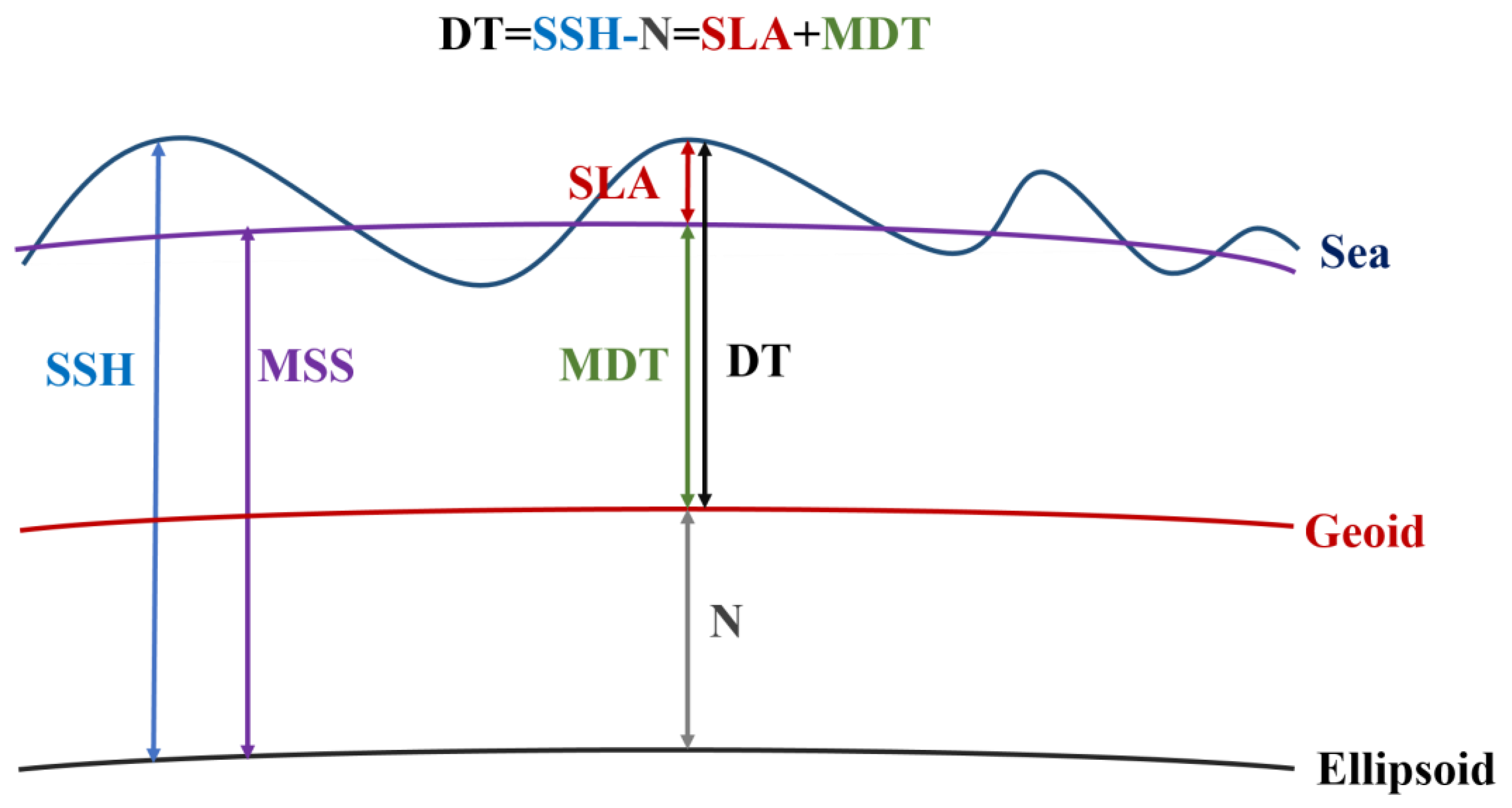
2.2. Determination of DT Using Two Different Schemes
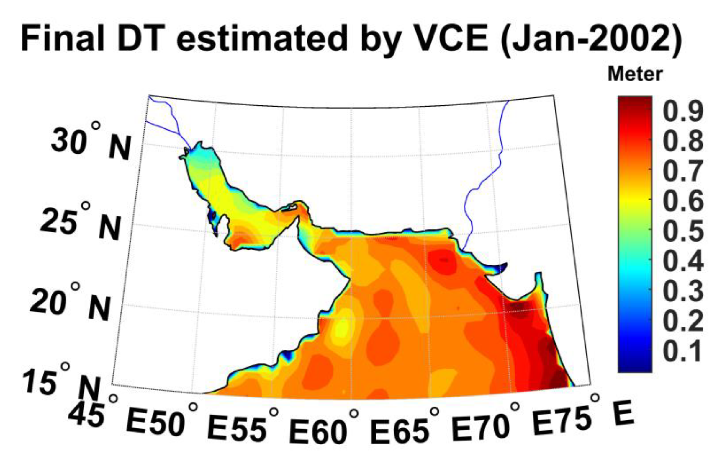
2.3. Assimilation Using Variance Component Estimation (VCE)
2.4. Assimilation Using Bayesian Theory Method
2.5. Assimilation Using Kalman Filter (KF)
2.6. Assimilation Using 3DVAR (3D Variational) Method
2.7. Estimation of Total Surface Current
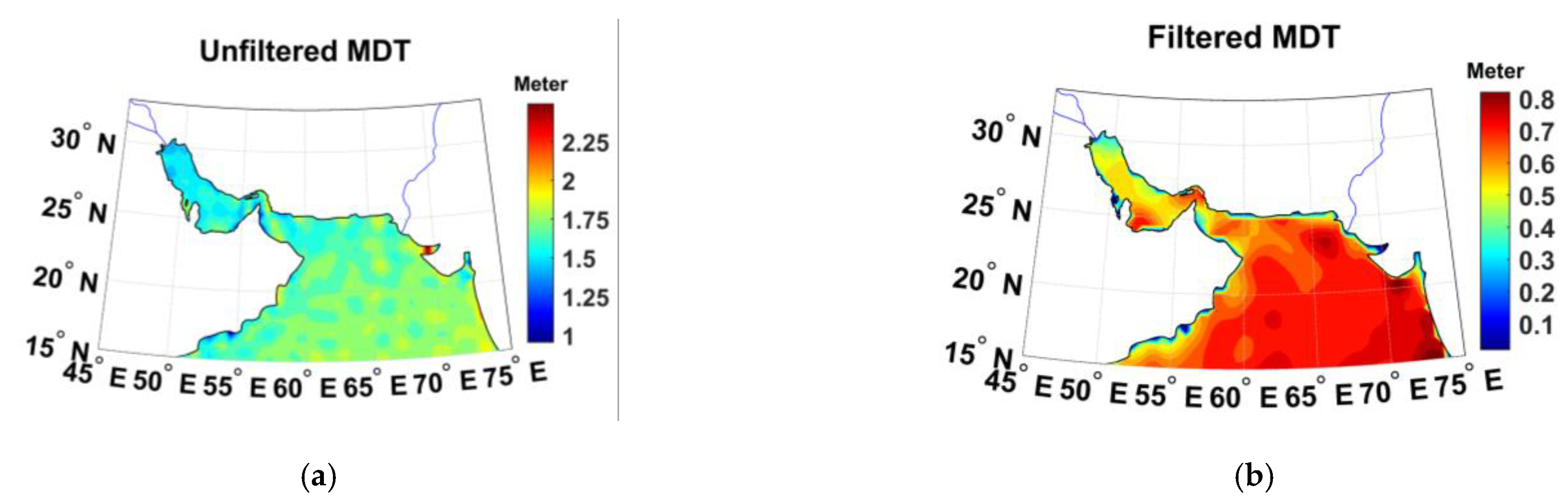
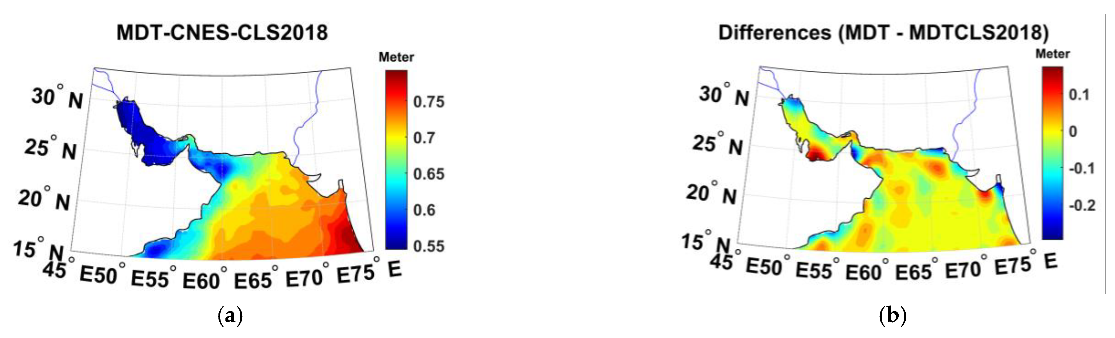
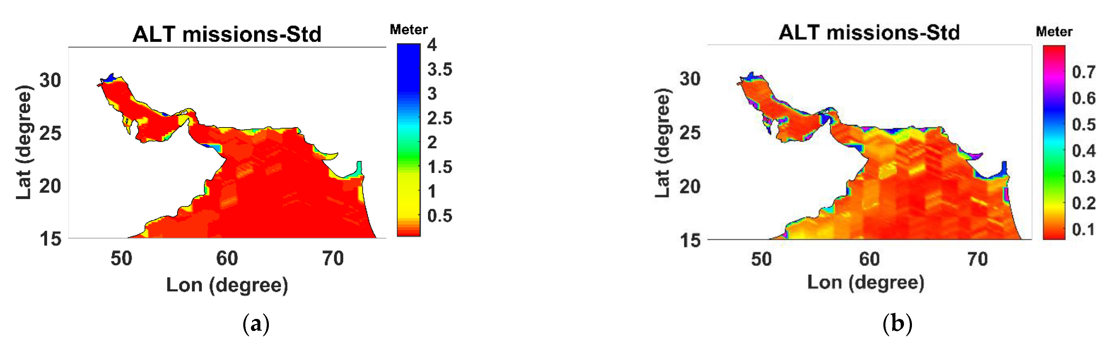
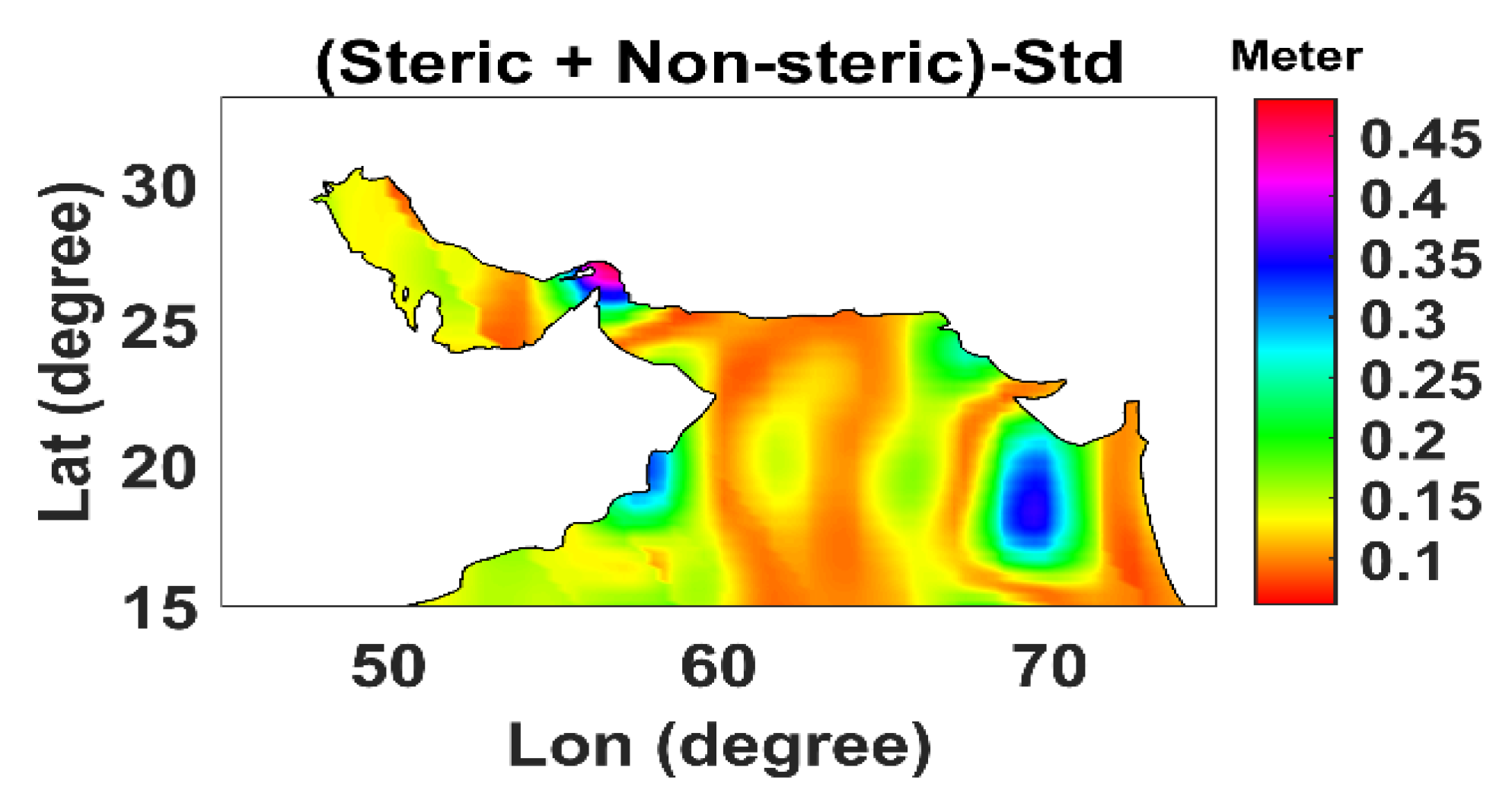
3. Results
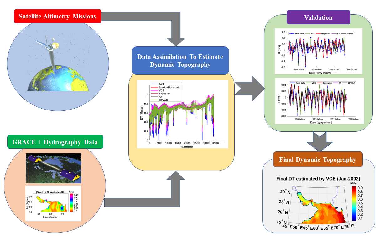
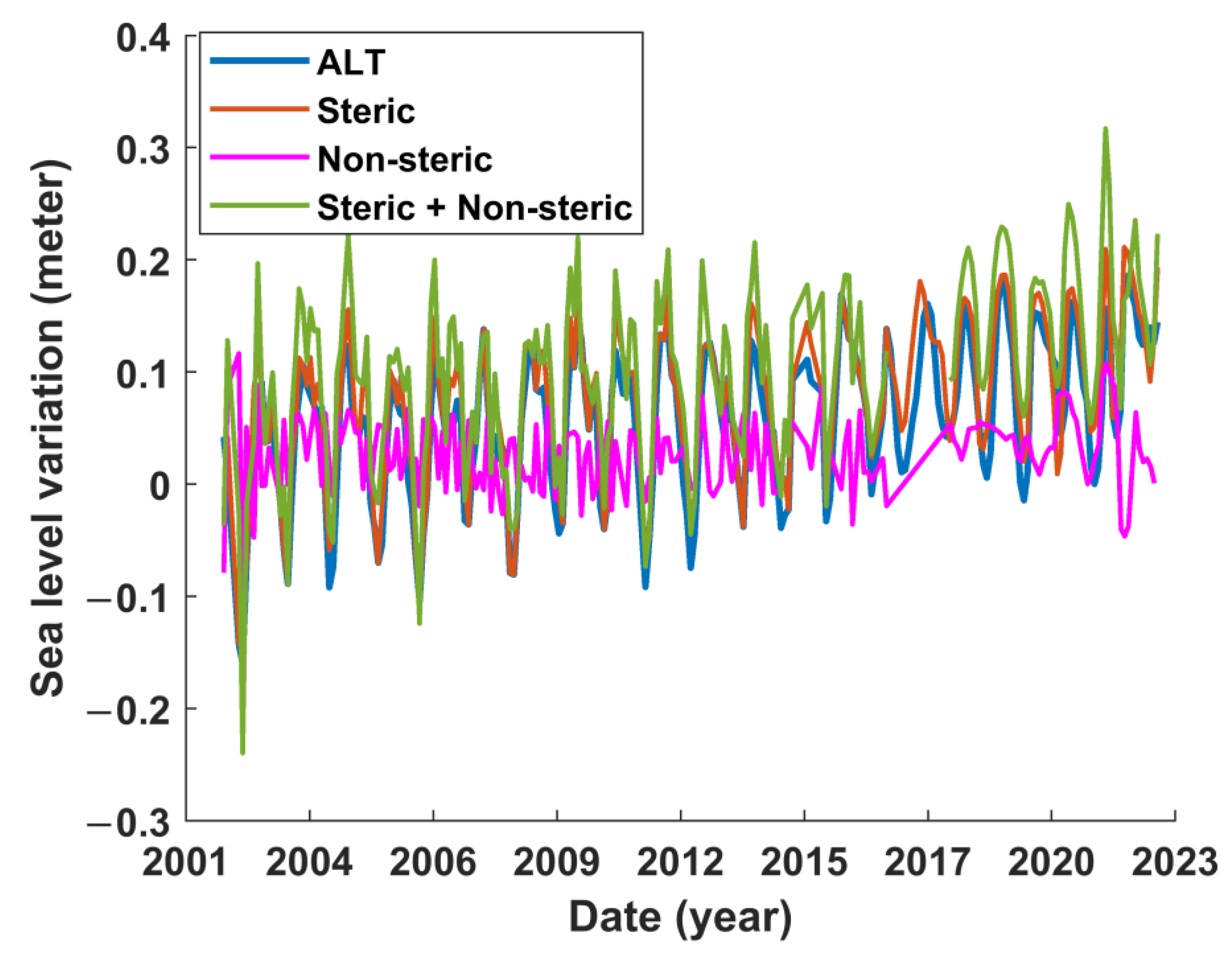
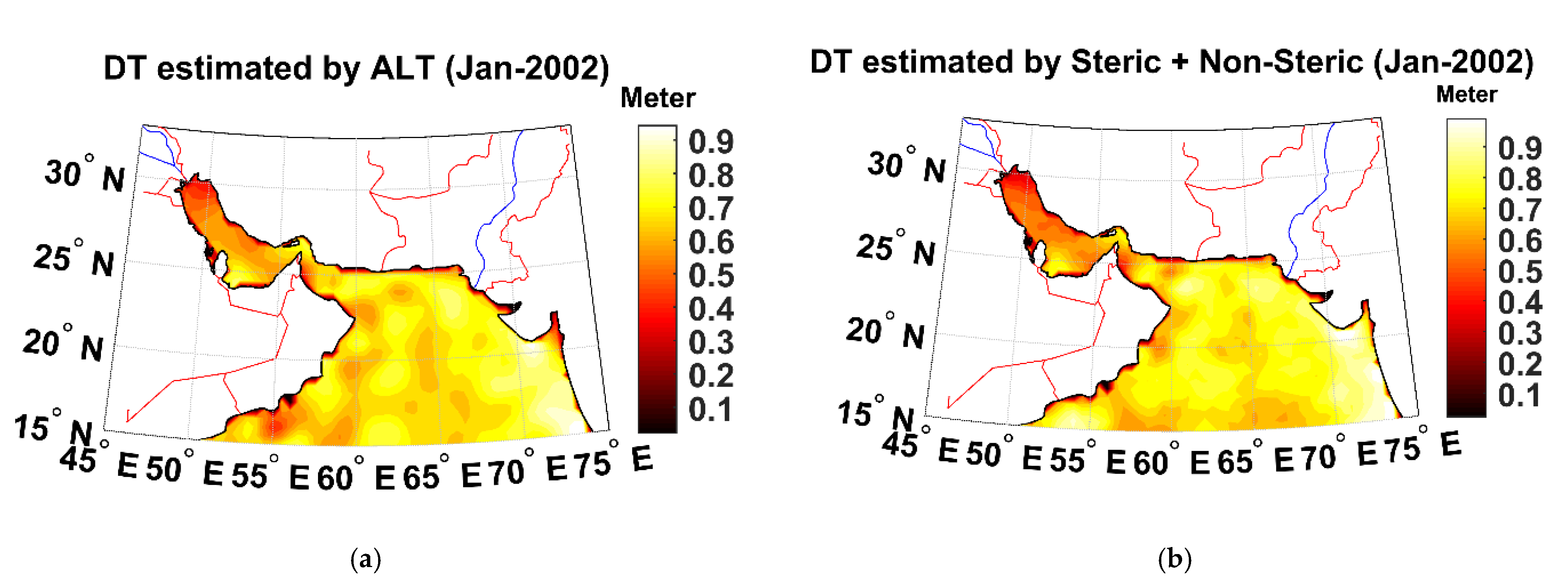
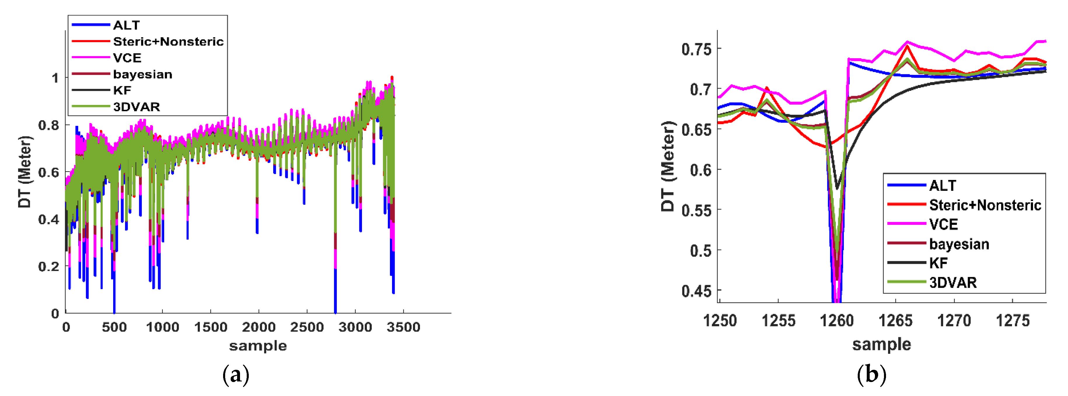
- DT is determined by employing satellite altimetry and integrating the steric and non-steric components of sea surface anomalies.
- Two different types of estimated DT are assimilated using the aforementioned approaches.
- The final DT is validated by comparing it with local current meter data.
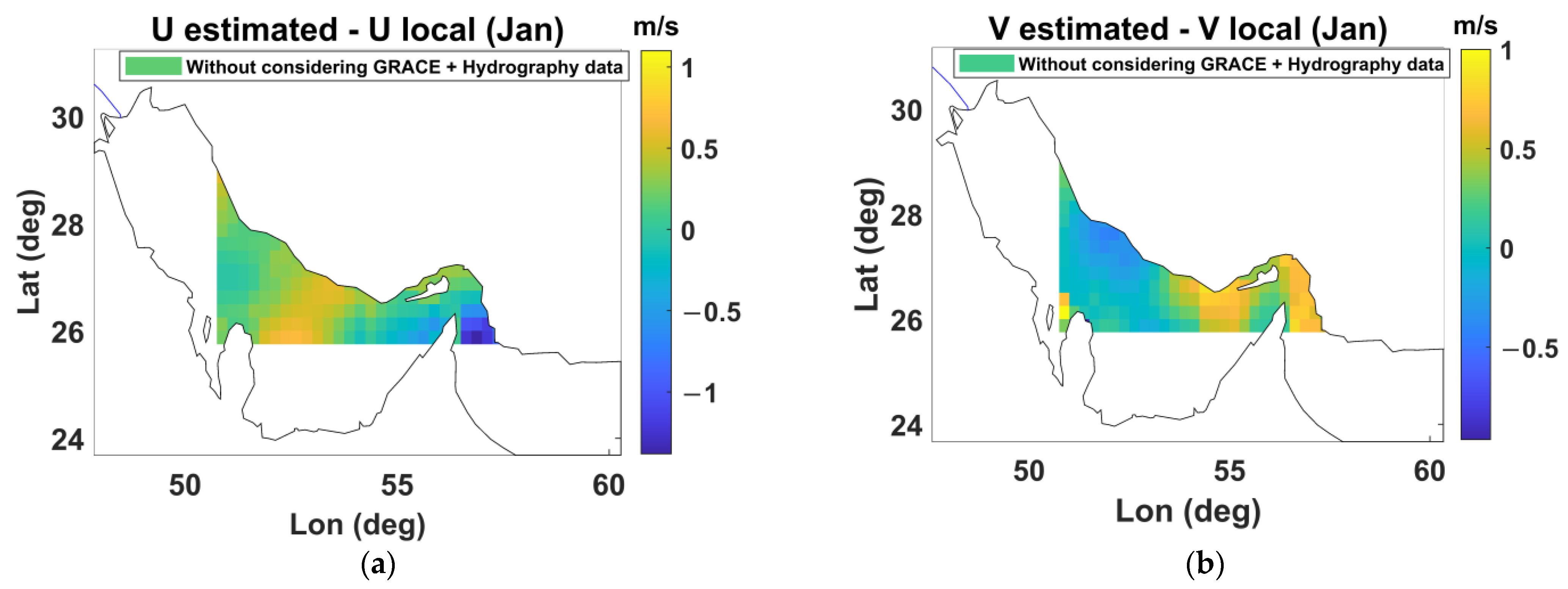
- (i).
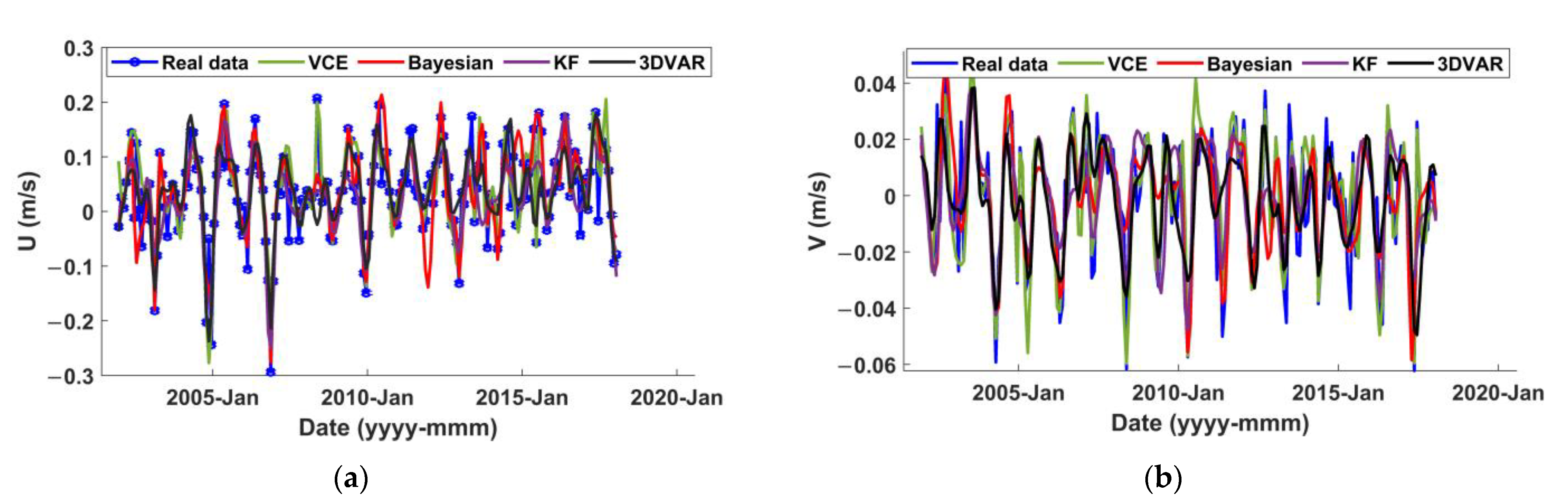
- Initially, the estimation of total surface currents solely relies on the DT obtained from altimetry observations, without incorporating GRACE and hydrographic data. Then, the estimated currents are compared against the measurements from the current meter.
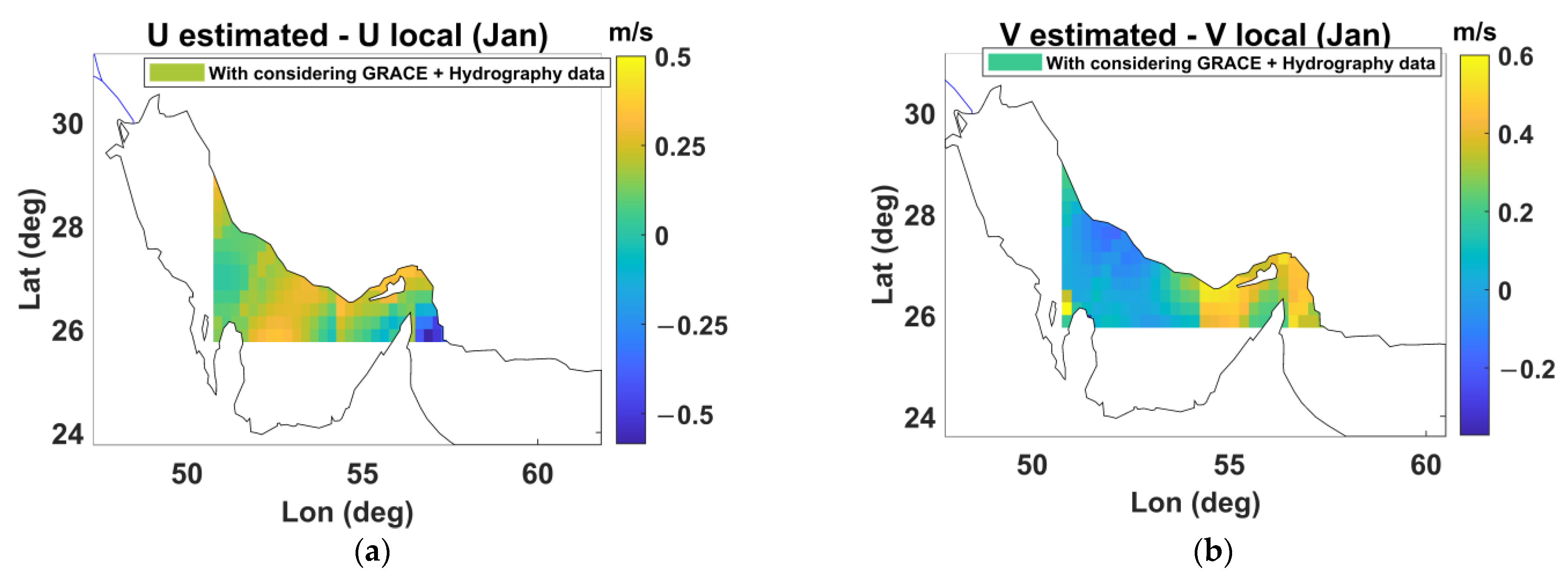
- (ii).
- Subsequently, the total surface currents are obtained by utilizing the DT derived from the combined datasets, which include altimetry satellites as well as GRACE and hydrographic data. Furthermore, the estimated currents are compared with the observations from the current meter.
4. Discussion
5. Conclusions
Author Contributions
Funding
Data Availability Statement
Conflicts of Interest
References
- Chelton, D.B.; Schlax, M.G. Global Observations of Oceanic Rossby Waves. Science 1996, 272, 234–238. [Google Scholar] [CrossRef]
- Buckingham, C.E.; Cornillon, P.C. The contribution of eddies to striations in absolute dynamic topography. J. Geophys. Res. Oceans 2013, 118, 448–461. [Google Scholar] [CrossRef]
- Moore, A.M.; Martin, M.J.; Akella, S.; Arango, H.G.; Balmaseda, M.; Bertino, L.; Ciavatta, S.; Cornuelle, B.; Cummings, J.; Frolov, S.; et al. Synthesis of Ocean Observations Using Data Assimilation for Operational, Real-Time and Reanalysis Systems: A More Complete Picture of the State of the Ocean. Front. Mar. Sci. 2019, 6, 90. [Google Scholar] [CrossRef]
- Kwok, R.; Morison, J. Dynamic topography of the ice-covered Arctic Ocean from ICESat. Geophys. Res. Lett. 2011, 38, L02501. [Google Scholar] [CrossRef]
- LeGrand, P.; O Schrama, E.J.; Tournadre, J. An inverse estimate of the dynamic topography of the ocean. Geophys. Res. Lett. 2003, 30, 1062. [Google Scholar] [CrossRef]
- Vergos, G.S.; Tziavos, I.N.; Sideris, M.G. On the Determination of Sea Level Changes by Combining Altimetric, Tide Gauge, Satellite Gravity and Atmospheric Observations. In Geodesy for Planet Earth. International Association of Geodesy Symposia; Kenyon, S., Pacino, M., Marti, U., Eds.; Springer: Berlin/Heidelberg, Germany, 2012; Volume 136. [Google Scholar] [CrossRef]
- Haines, B.; Desai, S.; Born, B. The Long-Term Altimeter Calibration Record from the Harvest Platform. 2014. Available online: http://www.aviso.oceanobs.com/fileadmin/documents/OSTST/2013/oral/Haines_harvest_2013.Pdf (accessed on 6 December 2023).
- Müller, S.; Brockmann, J.M.; Schuh, W.D. Consistent combination of gravity field, altimetry and hydrographic data. In Proceedings of the IAG Symposium, Gravity, Geoid and Height Systems (GGHS 2012), Venice, Italy, 9–12 October 2013; Marti, U., Ed.; Springer: Berlin/Heidelberg, Germany, 2014; Volume 141, pp. 267–273. [Google Scholar] [CrossRef]
- Feng, G.; Jin, S.; Zhang, T. Coastal sea level changes in Europe from GPS, tide gauge, satellite altimetry and GRACE, 1993–2011. Adv. Space Res. 2013, 51, 1019–1028. [Google Scholar] [CrossRef]
- Wang, G.; Cheng, L.; Boyer, T.; Li, C. Halosteric Sea Level Changes during the Argo Era. Water 2017, 9, 484. [Google Scholar] [CrossRef]
- Müller, F.L.; Dettmering, D.; Wekerle, C.; Schwatke, C.; Passaro, M.; Bosch, W.; Seitz, F. Ocean surface currents in the northern Nordic seas from a combination of multi-mission satellite altimetry and numerical modeling. In Proceedings of the EGU General Assembly 2020, Online, 4–8 May 2020. [Google Scholar] [CrossRef]
- Dettmering, D.; Schwatke, C.; Boergens, E.; Seitz, F. Potential of ENVISAT Radar Altimetry for Water Level Monitoring in the Pantanal Wetland. Remote Sens. 2016, 8, 596. [Google Scholar] [CrossRef]
- Castruccio, F.; Verron, J.; Gourdeau, L.; Brankart, J.; Brasseur, P. Joint altimetric and in-situ data assimilation using the GRACE mean dynamic topography: A 1993–1998 hindcast experiment in the tropical Pacific Ocean. Ocean Dyn. 2008, 58, 43–63. [Google Scholar] [CrossRef]
- Knudsen, P.; Bingham, R.; Andersen, O.; Rio, M.-H. A global mean dynamic topography and ocean circulation estimation using a preliminary GOCE gravity model. J. Geod. 2011, 85, 861–879. [Google Scholar] [CrossRef]
- Poulain, P.-M.; Menna, M.; Mauri, E. Surface Geostrophic Circulation of the Mediterranean Sea Derived from Drifter and Satellite Altimeter Data. J. Phys. Oceanogr. 2012, 42, 973–990. [Google Scholar] [CrossRef]
- Mangini, F.; Bonaduce, A.; Chafik, L.; Bertino, L. Validation of the ALES coastal altimetry dataset against the Norwegian tide gauges. In Proceedings of the EGU General Assembly 2021, Online, 19–30 April 2021. [Google Scholar] [CrossRef]
- Benveniste, J. Radar Altimetry: Past, Present and Future. Coastal Altimetry; Springer: Berlin/Heidelberg, Germany, 2010. [Google Scholar] [CrossRef]
- Chen, J.L.; Wilson, C.R.; Tapley, B.D.; Famiglietti, J.S.; Rodell, M. Seasonal global mean sea level change from satellite altimeter, GRACE, and geophysical models. J. Geod. 2005, 79, 532–539. [Google Scholar] [CrossRef]
- Pirooznia, M.; Naeeni, M.R.; Tourian, M.J. Modeling total surface current in the Persian Gulf and the Oman Sea by combination of geodetic and hydrographic observations and assimilation with in situ current meter data. Acta Geophys. 2023, 71, 2839–2863. [Google Scholar] [CrossRef]
- Bingham, R.J.; Haines, K.; Lea, D. A comparison of GOCE and drifter-based estimates of the North Atlantic steady-state surface circulation. Int. J. Appl. Earth Obs. Geoinf. 2014, 35, 140–150. [Google Scholar] [CrossRef]
- Chang, C.H.; Kuo, C.Y.; Shum, C.K.; Yi, Y.; Rateb, A. Global surface and subsurface geostrophic currents from multi-mission satellite altimetry and hydrographic data, 1996–2011. J. Mar. Sci. Technol. 2016, 24, 16. [Google Scholar] [CrossRef]
- Birol, F.; Brankart, J.M.; Castruccio, F.; Brasseur, P.; Verron, J. Impact of Ocean Mean Dynamic Topography on Satellite Data Assimilation. Mar. Geod. 2004, 27, 59–78. [Google Scholar] [CrossRef]
- Pirooznia, M.; Emadi, S.R.; Alamdari, M.N. The Time Series Spectral Analysis of Satellite Altimetry and Coastal Tide Gauges and Tide Modeling in the Coast of Caspian Sea. Open J. Mar. Sci. 2016, 06, 258–269. [Google Scholar] [CrossRef]
- Soltanpour, A.; Pirooznia, M.; Aminjafari, S.; Zareian, P. Persian gulf and Oman sea tide modeling using satellite altimetry and tide gauge data (TM-IR01). Mar. Georesources Geotechnol. 2017, 36, 677–687. [Google Scholar] [CrossRef]
- Pirooznia, M.; Naeeni, M.R. The application of least-square collocation and variance component estimation in crossover analysis of satellite altimetry observations and altimeter calibration. J. Oper. Oceanogr. 2020, 13, 100–120. [Google Scholar] [CrossRef]
- Bosch, W.; Dettmering, D.; Schwatke, C. Multi-Mission Cross-Calibration of Satellite Altimeters: Constructing a Long-Term Data Record for Global and Regional Sea Level Change Studies. Remote Sens. 2014, 6, 2255–2281. [Google Scholar] [CrossRef]
- Koblinsky, C.J.; Marsh, J.G. Satellite altimetry. In Geophysics. Encyclopedia of Earth Science; Springer: Boston, MA, USA, 1989. [Google Scholar] [CrossRef]
- Balmino, G. Efficient propagation of error covariance matrices of gravitational models: Application to GRACE and GOCE. J. Geod. 2009, 83, 989–995. [Google Scholar] [CrossRef]
- Xu, X.; Zhao, Y.; Reubelt, T.; Tenzer, R. A GOCE only gravity model GOSG01S and the validation of GOCE related satellite gravity models. Geodesy Geodyn. 2017, 8, 260–272. [Google Scholar] [CrossRef]
- Förste, C.; Bruinsma, S.; Abrikosov, O.; Rudenko, S.; Lemoine, J.M.; Marty, J.C.; Neumayer, K.H.; Biancale, R. EIGEN-6S4 A timevariable satellite-only gravity field model to d/o 300 based on LAGEOS, GRACE and GOCE data from the collaboration of GFZ Potsdam and GRGS Toulouse. V. 2.0. GFZ Data Serv. 2016. [Google Scholar] [CrossRef]
- Fecher, T.; Pail, R.; Gruber, T. GOCO05c: A New Combined Gravity Field Model Based on Full Normal Equations and Regionally Varying Weighting. Surv. Geophys. 2017, 38, 571–590. [Google Scholar] [CrossRef]
- Ries, J.; Bettadpur, S.; Eanes, R.; Kang, Z.; Ko, U.; McCullough, C.; Nagel, P.; Pie, N.; Poole, S.; Richter, T.; et al. The combined gravity model GGM05C. GFZ Data Serv. 2016. [Google Scholar] [CrossRef]
- Förste, C.; Bruinsma, S.L.; Abrikosov, O.; Lemoine, J.M.; Marty, J.C.; Flechtner, F.; Balmino, G.; Barthelmes, F.; Biancale, R. EIGEN-6C4 the latest combined global gravity field model including GOCE data up to degree and order 2190 of GFZ Potsdam and GRGS Toulouse. GFZ Data Serv. 2014. [Google Scholar] [CrossRef]
- Zingerle, P.; Pail, R.; Gruber, T.; Oikonomidou, X. The combined global gravity field model XGM2019e. J. Geod. 2020, 94, 66. [Google Scholar] [CrossRef]
- Jayne, S.R.; Wahr, J.M.; Bryan, F.O. Observing Ocean heat content using satellite gravity and altimetry. J. Geophys. Res. Oceans 2003, 108, 13. [Google Scholar] [CrossRef]
- Jimenez-Gonzalez, S.; Mayerle, R.; Egozcue, J.J. On the accuracy of acoustic Doppler current profilers for in-situ measurements. A proposed approach and estimations for measurements in tidal channels. In Proceedings of the IEEE/OES Seventh Working Conference on Current Measurement Technology, San Diego, CA, USA, 13–15 March 2003; pp. 197–201. [Google Scholar] [CrossRef]
- Pirooznia, M.; Naeeni, M.R.; Amerian, Y. A Comparative Study Between Least Square and Total Least Square Methods for Time–Series Analysis and Quality Control of Sea Level Observations. Mar. Geodesy 2019, 42, 104–129. [Google Scholar] [CrossRef]
- Raj, R.P. Surface velocity estimates of the North Indian Ocean from satellite gravity and altimeter missions. Int. J. Remote Sens. 2016, 38, 296–313. [Google Scholar] [CrossRef]
- Han, D.; Wahr, J. The viscoelastic relaxation of a realistically stratified earth, and a further analysis of postglacial rebound. Geophys. J. Int. 1995, 120, 287–311. [Google Scholar] [CrossRef]
- Amiri-Simkooei, A.R.; Tiberius, C.C.; Teunissen, P.J. Assessment of noise in GPS coordinate time series: Methodology and results. J. Geophys. Res. 2007, 112, B07413. [Google Scholar] [CrossRef]
- Zhou, T.; Chen, M.; Yang, C.; Nie, Z. Data fusion using Bayesian theory and reinforcement learning method. Sci. China Inf. Sci. 2020, 63, 170209. [Google Scholar] [CrossRef]
- Garcia-Huerta, R.A.; González-Jiménez, L.E.; Villalon-Turrubiates, I.E. Sensor Fusion Algorithm Using a Model-Based Kalman Filter for the Position and Attitude Estimation of Precision Aerial Delivery Systems. Sensors 2020, 20, 5227. [Google Scholar] [CrossRef]
- Liu, Y.; Li, L.; Yang, J.; Chen, X.; Hao, J. Estimating Snow Depth Using Multi-Source Data Fusion Based on the D-InSAR Method and 3DVAR Fusion Algorithm. Remote Sens. 2017, 9, 1195. [Google Scholar] [CrossRef]
- Ide, K.; Courtier, P.; Ghil, M.; Lorenc, A.C. Unified Notation for Data Assimilation: Operational, Sequential and Variational (gtSpecial IssueltData Assimilation in Meteology and Oceanography: Theory and Practice). J. Meteorol. Soc. Jpn. Ser. II 1997, 75, 181–189. [Google Scholar] [CrossRef]
- Sudre, J.; Maes, C.; Garçon, V. On the global estimates of geostrophic and Ekman surface currents. Limnol. Oceanogr. Fluids Environ. 2013, 3, 1–20. [Google Scholar] [CrossRef]
- Rio, M.; Hernandez, F. A mean dynamic topography computed over the world ocean from altimetry, in situ measurements, and a geoid model. J. Geophys. Res. 2004, 109, C12032. [Google Scholar] [CrossRef]
- Bruinsma, S.L.; Förste, C.; Abrikosov, O.; Lemoine, J.; Marty, J.; Mulet, S.; Rio, M.; Bonvalot, S. ESA’s satellite-only gravity field model via the direct approach based on all GOCE data. Geophys. Res. Lett. 2014, 41, 7508–7514. [Google Scholar] [CrossRef]


| Missions | Cycles | Periods | Sources | Accuracy Value |
|---|---|---|---|---|
| Jason 1 | 001-259 | 15 January 2002–16 January 2009 | NASA, AVISO | about 4 cm |
| Jason 2 | 001-303 | 4 July 2008–1 October 2016 | AVISO | about 4 cm |
| Jason 3 | 001-050 | 18 February 2016–12 June 2017 | AVISO | about 4 cm |
| Envisat | 008-093 | 23 July 2002–18 October 2010 | ESA | about 3 cm |
| Saral | 001-035 | 14 March 2013–16 June 2016 | AVISO | about 8 cm |
| Sentinel3A | 001-083 | 16 March 2016–3 January 2023 | ESA | about 3 cm |
| Sentinel3B | 001-057 | 4 June 2018–13 January 2023 | ESA | about 3 cm |
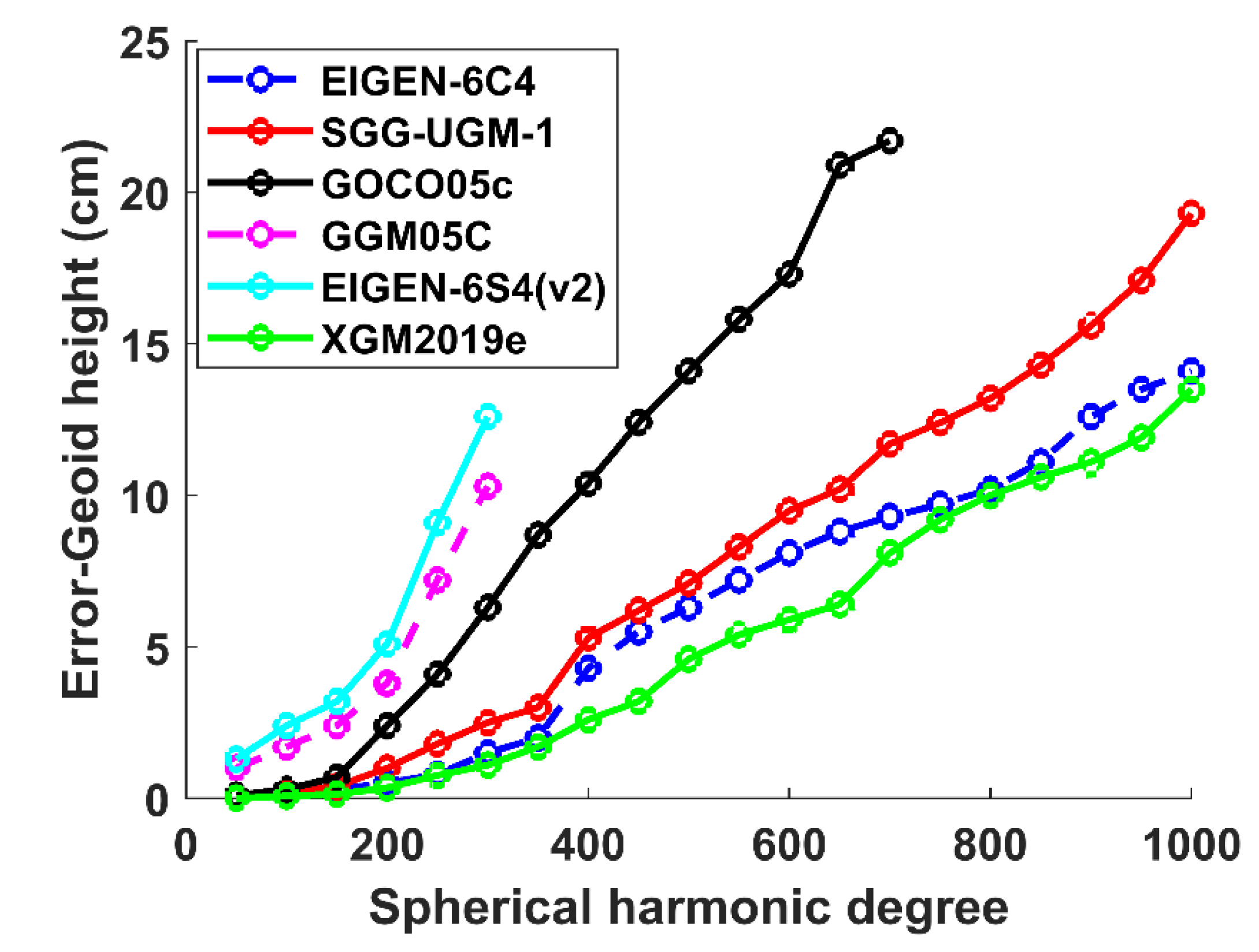
| Numbers | Models | Produced Year | Degree Count | Data Source | References |
|---|---|---|---|---|---|
| 1 | SGG-UGM-1 | 2018 | 2159 | EGM2008, S(GOCE) | [29] |
| 2 | EIGEN-6S4 (v2) | 2016 | 300 | S(GOCE), S(GRACE), S(LAGEOS) | [30] |
| 3 | GOCO05c | 2016 | 720 | A, G, S | [31] |
| 4 | GGM05C | 2015 | 360 | A, G, S(GOCE), S(GRACE) | [32] |
| 5 | EIGEN-6C4 | 2014 | 2190 | A, G, S(GOCE), S(GRACE), S(LAGEOS) | [33] |
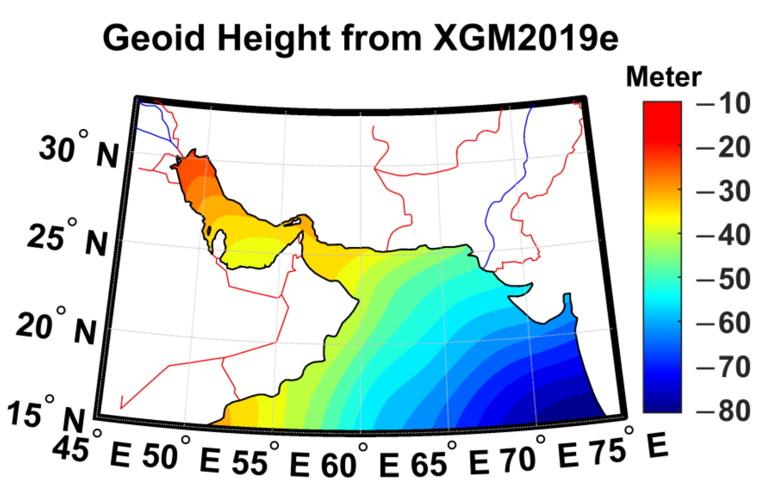
| 6 | XGM2019e | 2019 | 5399 | A, G, S(GOCO06s), T (Topography) | [34] |
| Number | Region | Equipment | Locations (Lat, Lon) | Periods | Sources |
|---|---|---|---|---|---|
| 1 | Khuran | ADCP | 26.7, 55.45 | 30 August 2005–10 April 2005 | INIO |
| 2 | Konarak | ADCP | 25.37, 60.43 | 21 August 2006–9 March 2007 | PMO |
| 3 | Chabahar | ADCP | 25.29, 60.47 | 21 August 2006–9 March 2007 | PMO |
| 4 | Bushehr | ADCP | 28.97, 50.66 | 15 June 2010–26 July 2011 | PMO |
| 5 | Taheri | ADCP | 27.63, 52.36 | 23 August 2008–24 September 2009 | PMO |
| 6 | Nayband Gulf | ADCP | 27.42, 52.65 | 5 November 2009–7 December 2009 | PMO |
| 7 | Nakhl Taghi | ADCP | 27.49, 52.57 | 22 August 2008–24 September 2009 | PMO |
| 8 | Kangan | ADCP | 27.83, 52.04 | 23 August 2008–25 September 2009 | PMO |
| 10 | Jask | ADCP | 25.65, 57.76 | 16 July 2010–23 January 2011 | PMO |
| 11 | Larak | ADCP | 26.82, 56.37 | 10 June 2009–10 December 2010 | PMO |
| 12 | Googsar | ADCP | 25.60, 57.77 | 7 December 2010–28 October 2010 | PMO |
| 13 | Rajaei | ADCP | 27.07, 56.08 | 10 December 2009–1 December 2010 | PMO |
| Station Name | VCE | Bayesian | Kalman Filter | 3DVAR |
|---|---|---|---|---|
| Khoran | 12.15 | 12.25 | 17.30 | 23.65 |
| Konarak | 12.01 | 11.14 | 13.22 | 16.15 |
| Chabahar | 18.23 | 16.33 | 12.41 | 30.41 |
| Bushehr | 13.33 | 17.53 | 14.57 | 41.26 |
| Taheri | 17.21 | 23.34 | 20.43 | 38.55 |
| Nayband | 12.41 | 27.35 | 16.46 | 31.62 |
| Nakhl-Taghi | 10.42 | 12.23 | 10.34 | 26.75 |
| Kangan | 11.44 | 15.32 | 15.30 | 40.54 |
| Jask | 18.32 | 11.12 | 20.43 | 22.19 |
| Larak | 11.47 | 22.52 | 16.55 | 50.53 |
| Googsar | 16.43 | 13.51 | 20.51 | 44.79 |
| Rajaei | 14.20 | 10.36 | 11.52 | 37.31 |
Disclaimer/Publisher’s Note: The statements, opinions and data contained in all publications are solely those of the individual author(s) and contributor(s) and not of MDPI and/or the editor(s). MDPI and/or the editor(s) disclaim responsibility for any injury to people or property resulting from any ideas, methods, instructions or products referred to in the content. |
© 2024 by the authors. Licensee MDPI, Basel, Switzerland. This article is an open access article distributed under the terms and conditions of the Creative Commons Attribution (CC BY) license (https://creativecommons.org/licenses/by/4.0/).
Share and Cite
Pirooznia, M.; Voosoghi, B.; Poreh, D.; Amini, A. Integrating Hydrography Observations and Geodetic Data for Enhanced Dynamic Topography Estimation. Remote Sens. 2024, 16, 527. https://doi.org/10.3390/rs16030527
Pirooznia M, Voosoghi B, Poreh D, Amini A. Integrating Hydrography Observations and Geodetic Data for Enhanced Dynamic Topography Estimation. Remote Sensing. 2024; 16(3):527. https://doi.org/10.3390/rs16030527
Chicago/Turabian StylePirooznia, Mahmoud, Behzad Voosoghi, Davod Poreh, and Arash Amini. 2024. "Integrating Hydrography Observations and Geodetic Data for Enhanced Dynamic Topography Estimation" Remote Sensing 16, no. 3: 527. https://doi.org/10.3390/rs16030527