Technical Note

Aerial Drone Imaging in Alongshore Marine Ecosystems: Small-Scale Detection of a Coastal Spring System in the North-Eastern Adriatic Sea

National Institute of Oceanography and Applied Geophysics—OGS, 34010 Trieste, Italy
*
Author to whom correspondence should be addressed.
Remote Sens. 2023, 15(19), 4864; https://doi.org/10.3390/rs15194864
Submission received: 4 August 2023 / Revised: 5 October 2023 / Accepted: 5 October 2023 / Published: 7 October 2023

Abstract

:
The eastern coastline of the Gulf of Trieste (north-eastern Adriatic Sea, Italy) is characterized by the occurrence of coastal and submarine freshwater springs of karstic origin. In one of these areas, we performed a survey with a drone with a thermal camera installed, in tandem with in situ oceanographic sampling with a CTD. Drone images revealed a small time-space scale (i.e., up to a few meters) phenomenon of freshwater plumes floating over seawater. Comparing sea surface temperature data with those acquired in situ revealed that the phenomenon was not clearly detectable by the classical oceanographic monitoring, this surface spring freshwater layer being too thin. Instead, the drone’s thermal camera detected these dynamics with great accuracy, indicating that aerial drones can be efficiently used for studying fine-scale events involving surface waters (e.g., spills/pollution). The experience gained allowed us to discuss some of the advantages and disadvantages of using drone thermal imaging for monitoring alongshore areas.

1. Introduction

Coastal zones are strikingly complex and dynamic environments, markedly impacted by both natural phenomena and anthropogenic pressures. Coastal monitoring is a pivotal tool for the sustainable management of these areas, in order to ensure the maintenance of the essential ecosystem services they provide.
The classical monitoring by boat is a cornerstone for oceanographic studies, especially when aiming to investigate the properties of the water column. Nonetheless, coastal monitoring can be problematic, particularly when it comes to studying phenomena occurring alongshore and at a small spatial scale (i.e., up to a few meters). Indeed, approaching the coastline by boat is often challenging, especially when the shore is shallow or rocky. Additionally, the movements of the boat can alter the properties of the surface water under investigation, thus modifying the small-scale features.
Alternative techniques hold the potential to overcome these issues to some extent, thus complementing the data acquired by the boat, yet limited to the sea surface. Monitoring via remote sensing (i.e., satellites, aircrafts, aerial drones, etc.) allows us to detect at a distance the physical characteristics of the surface of interest.
Satellite systems provide synoptic images, with large area coverage, multispectral imaging and a quite frequent revisit time; however, the spatial resolution of the images freely available online is usually not suitable for studying phenomena that need to be analyzed in great detail [1]: for instance, the resolution of ESA’s Sentinel Copernicus is up to 10 m [2], and that of NASA’s Landsat is up to 15 m [3]. Consequently, in cases of studies being performed near- or along-shore, the elevated heterogeneity of the ground (a mixture of rocks, water, trees, buildings, etc.) is not resolved by the minimum mapping unit, which affects the quality of the acquired imagery and the possibility to detect fine-scale details. Finally, cloud coverage and weather conditions can hinder the acquisition of images of the surface of interest, making them unusable and nullifying monitoring efforts.
Manned aircrafts can provide images with higher spatial resolution and allow for a higher customizability in planning the monitoring, but are often characterized by low operational flexibility, temporariness, and high prices [4]. For these reasons, other existing and more versatile techniques are crucial for expanding our knowledge of the dynamics of alongshore waters at the desired spatial resolution.
Remote sensing by unmanned aerial vehicles (UAVs) (commonly known as aerial drones) allows us to generate data with ultra-high spatial resolution (<10 cm) over relatively small spatial extents, thanks to the low operating altitude, and with operator-determined revisit times [1,5]. In recent years, this technique has developed widely, with large applications worldwide for both research and operational monitoring purposes, also due to the increasing variety of associated miniaturized sensors [1,5,6,7]. Among these sensors, UAVs equipped with thermal cameras can now ensure the acquisition of thermal images (TIR, i.e., thermal infrared) with sub-metric resolution, enabling the detection of fine-scale phenomena [4,7,8]. Several works have used TIR-imaging by drone for studying the coastal discharge of groundwater or geothermal fluids [4,8,9,10]. The desirable conditions to carry out TIR measurements would be at low light intensities (dawn/sunset) or even at night and in good weather, to prevent issues related to the intrinsic variability of meteorological conditions (wind and cloud movements can induce light variations), which introduce additional variability into the acquired data. However, this is hardly feasible and most studies (see for example [8,9]) are performed in the daytime to meet the operational needs.
The aim of this technical paper is to showcase the usability of an aerial drone for detecting and mapping fine-scale surface oceanographic dynamics in a peculiar alongshore marine environment and, ultimately, to provide useful guidelines for alongshore monitoring via drone. The area of study is known for being characterized by freshwater springs [11,12], but this is the first time such a new technology has been applied there. We compared the sea surface temperature acquired with a thermal camera mounted on a drone with data collected by a classical in situ oceanographic sampling with a CTD. The results allowed us to depict features never observed before and to resolve the complicated dynamics of the area. The experience gained let us discuss some of the advantages and disadvantages of using drone thermal imaging for monitoring alongshore areas.

2. Materials and Methods

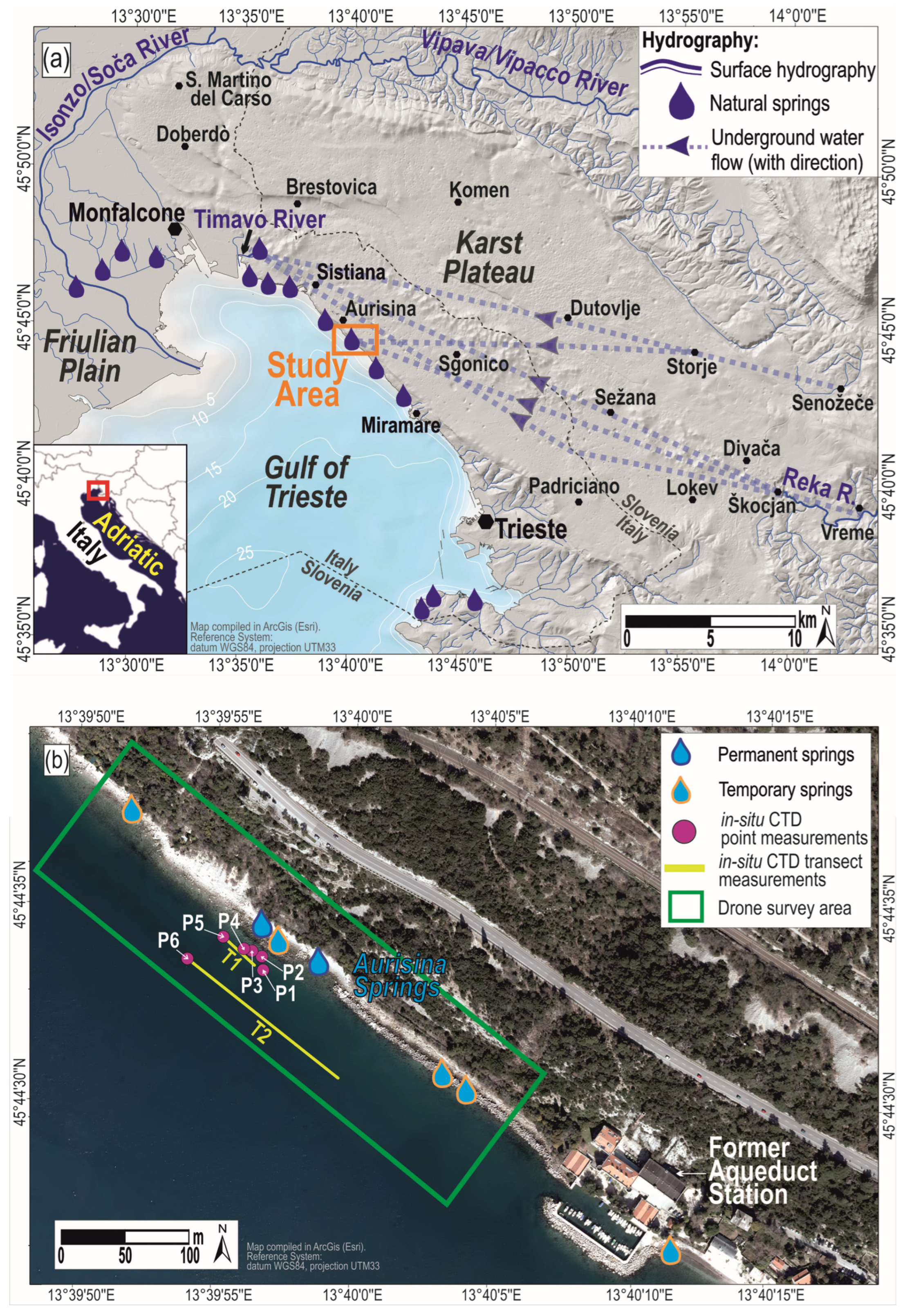
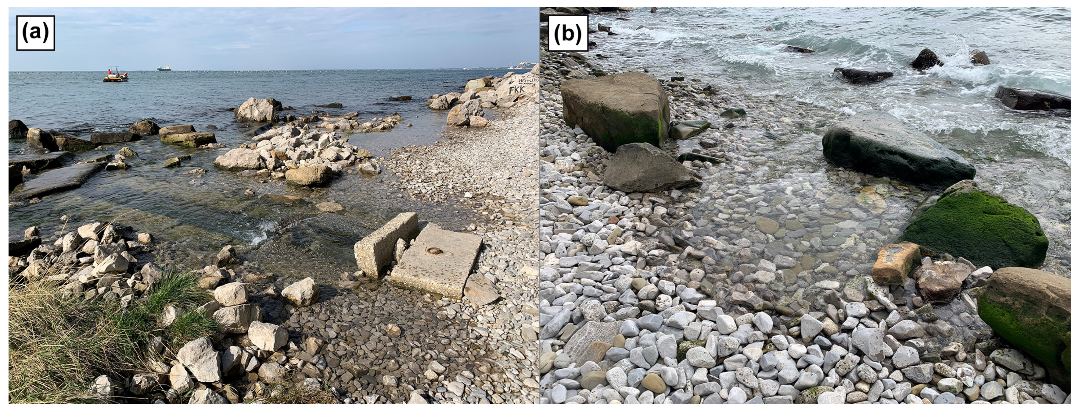
2.1. Study Area and Site
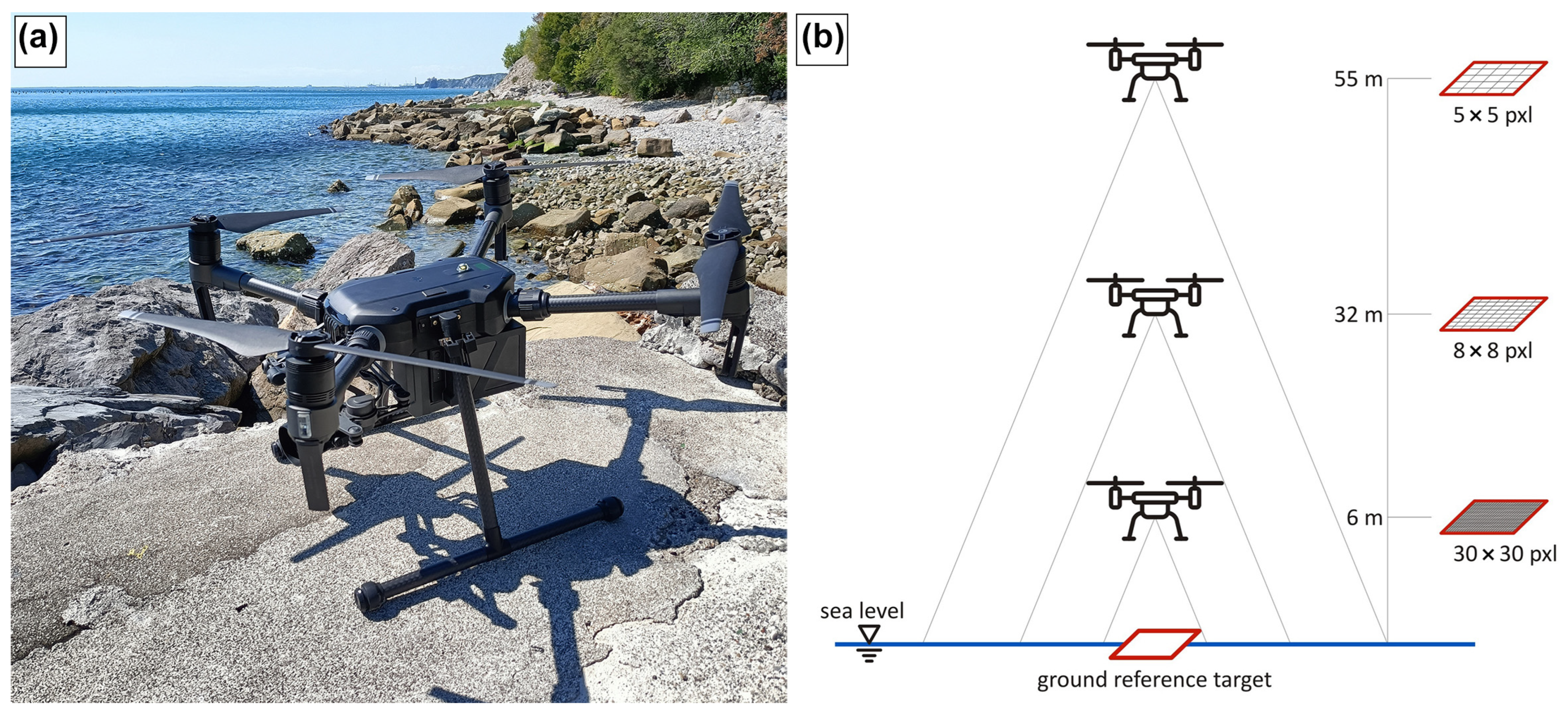
The study area lays along the eastern coastline of the Gulf of Trieste (north-eastern Adriatic Sea, Mediterranean Sea), at the flank of the Karst Plateau (Figure 1a).
The Karst Plateau consists of Meso-Cenozoic carbonates that have a high permeability due to intense karstification and fracture systems, with sinkholes and widespread infiltration feeding the underground aquifer. One of the most important features of the Karst aquifer is the Reka River, which sinks after 55 km at Škocjan (Slovenia) and becomes the underground Timavo River that reappears after 34 km, at the NW tip of the Karst [12].
The Eocene flysch, consisting of sands and marls, covers the flanks of the Karst Plateau, and constitutes a low permeability barrier to the aquifer, especially along the southern coast. In fact, the main coastal and submarine springs, which represent the leakage of the karst aquifer, are located in the northern part of the coast where the flysch/limestone contact is at or below the sea level [11,12].
The main leakage sites are: (i) in the north-west, the Timavo’s one, characterized by four springs with a flow rate of about 30 m3/s; (ii) in the south-east, the Aurisina’s one, characterized by several springs along 350 m long coastline, with an average flow rate of 0.3 m3/s [12] (Figure 1a). The freshwater of the karstic aquifer at the Timavo and Aurisina springs has an average temperature of 12 °C, ranging from 11 °C (with minima of 9 °C) in winter, to 13 °C in summer [12]. Notably, the Aurisina springs were used from 1855 to 1971 to feed the aqueduct supplying the city of Trieste. Between these two main sites, there are many smaller coastal springs identified by [11].
The study site is located at the Aurisina springs (45°44′34″N, 13°39′57.3″E) and encompasses about 200 m along the shore (Figure 1b), with two main natural permanent springs visible on the beach constituted by pebbles (Figure 2) and other temporary springs as reported by [12] and from direct observations. Of the two permanently active springs, the northernmost spring outlet is regulated by an artificial channel about 40 cm large, 50 cm deep, and 8 m long that ends at the artificial rock barrier of the beach (Figure 2a), the southernmost flows naturally along the beach from a front ca. 3 m long located approximately at the sea level, and visible during low tide (Figure 2b). At the monitoring time (10 October 2022), spring water was colder than seawater, the weather conditions were stable and the cloud coverage was uniform.

2.2. Aerial Drone

The aerial survey was conducted using a DJI Matrice 210 v2 drone equipped with a high-resolution (640 × 512 pixels) DJI XT2 thermal imaging camera, which couples a FLIR longwave infrared thermal camera and a visual camera, providing both infrared and visible light imaging simultaneously (Figure 3a). The FLIR longwave infrared camera is equipped with an uncooled VOx microbolometer and provides high-sensitivity (<50 mK @ f/1.0) infrared scanning in the spectral range 7.5–13.5 µm, while the visual camera captures 4 K videos and 12 MP photos. During post-processing, the pixel values of the acquired thermal images were converted to temperature values in °C using the following formula:
Temperature (°C) = S × 0.04 − 273.15,
where S is the value of the pixel stored in the raw file and 0.04 is the correction coefficient linked to the setting of the camera’s shooting thermal range [15].
To understand if there was any effect of the flight altitude on the sea surface temperature detected by the thermal camera, a fixed ground reference target square of 0.5 m2 at the freshwater spring outlet was considered. The mean temperature value therein (i.e., Tf) was then compared among the different altitudes (Figure 3b). The same test was performed on a comparable area on land, at fixed altitude intervals, to understand if any differences found on the sea surface were due to the altitude.
The thermal images acquired at the different altitudes and converted during post-processing were then corrected, to best merge them and, thus, to obtain a larger view of the area of interest at the highest spatial resolution. The correction also allowed us to obtain maps with realistic sea surface temperature values, going beyond just identifying thermal contrasts. For each altitude, the corrective factor (CF) was determined as
CF (°C) = Tf − Tr,
where Tf is the mean temperature value measured at the fixed reference square of 0.5 m2 at the freshwater spring outlet, and Tr is the real temperature measured in situ at the same location (see Section 2.3 for details). The obtained CF was thus applied to all the pixels of the image.
Recognizable natural elements (considered as ground control points, GCPs) alongshore (e.g., boulders, wharfs) were extracted from true orthophotos [13] with a GSD (Ground Sample Distance) of 25 cm, and LIDAR data of comparable resolution (15–20 cm) of property of our Institute (National Institute of Oceanography and Applied Geophysics—OGS). So, we can assume that the accuracy of georectification is equivalent to that of orthophotos (i.e., 25 cm).
The detection of GCPs for orthorectification and mosaicking of the images was carried out using 3DF Zephyr, a commercial software for photogrammetry and 3D modelling [16].

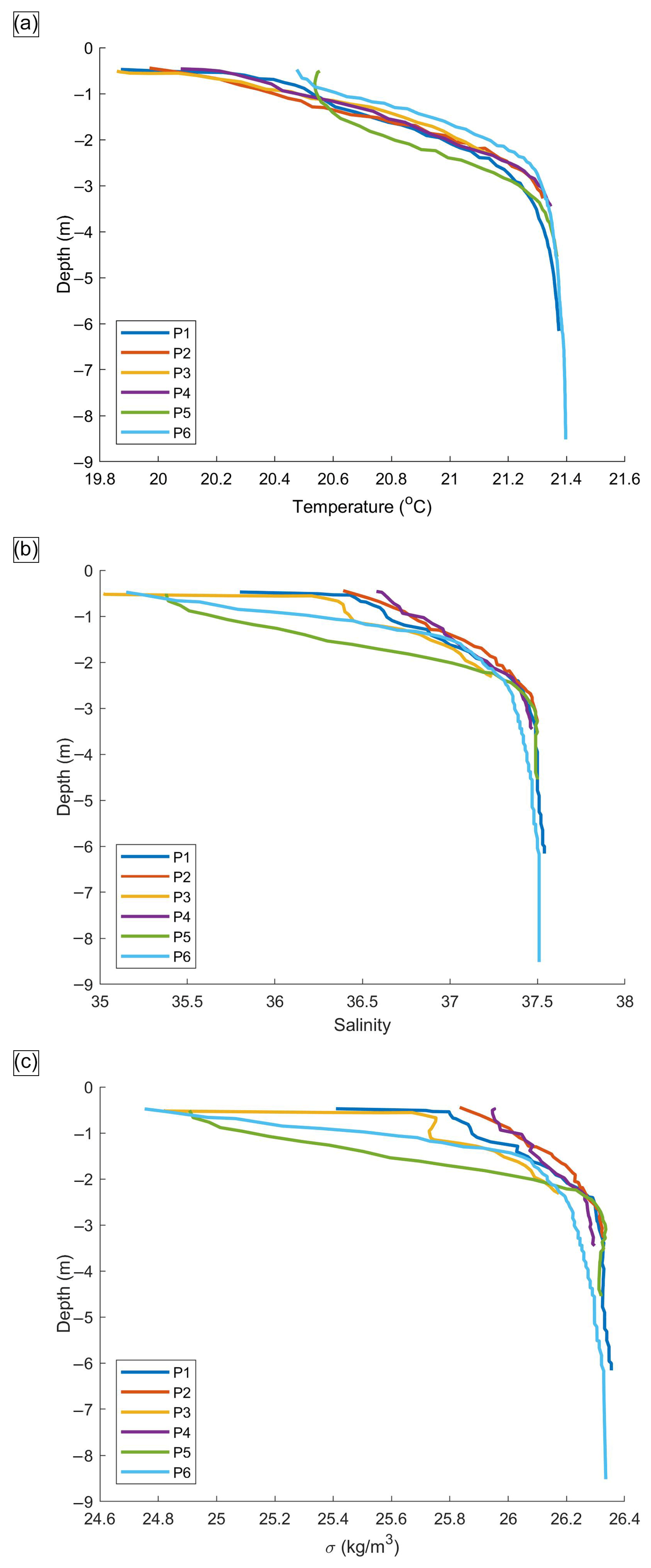
2.3. Oceanographic Monitoring
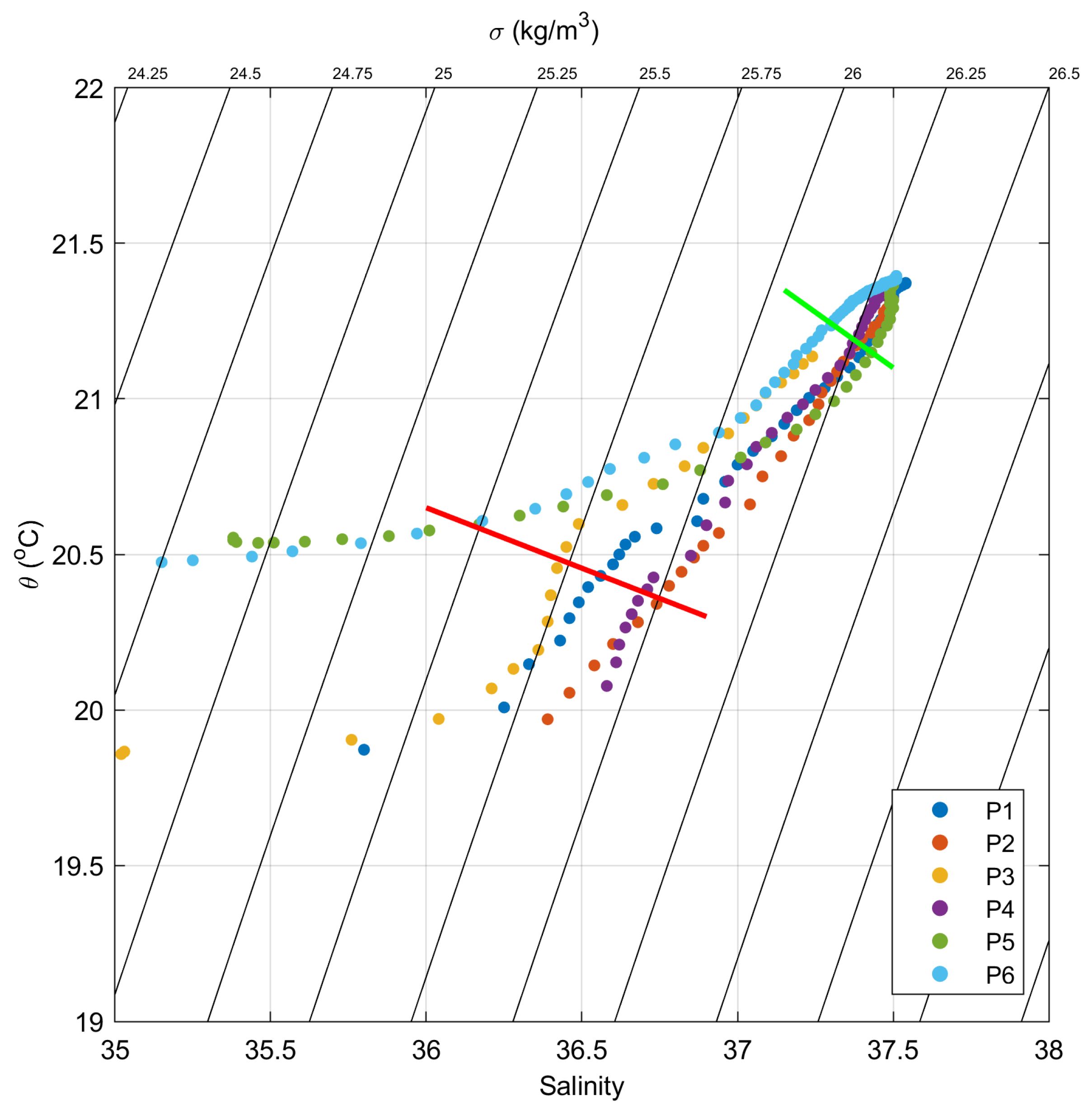
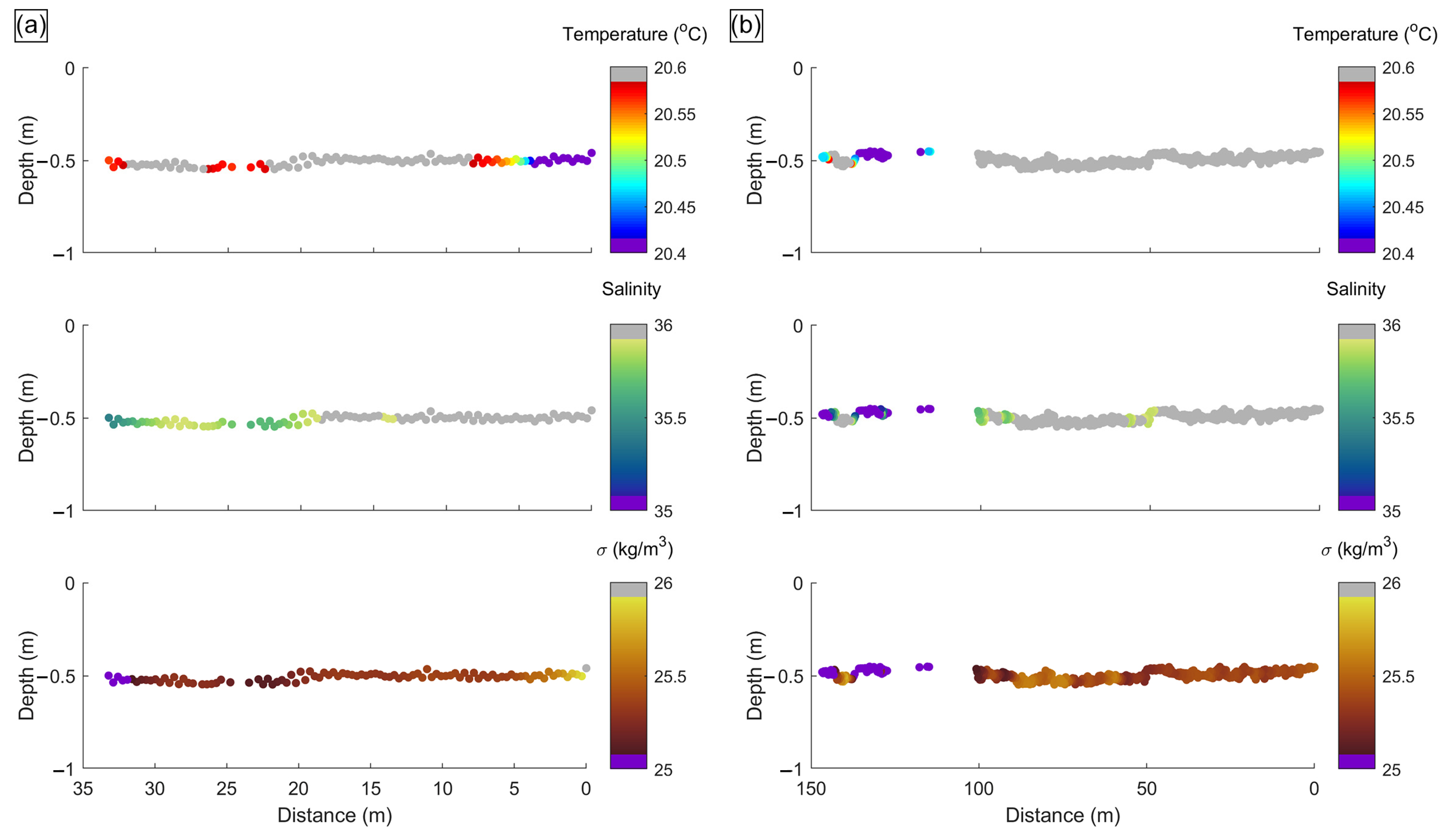
Oceanographic data were collected in tandem with drone flights over the study area. Measurements were performed with two multiparametric probes (YSI Professional Plus (Pro Plus) Multiparameter Meter at the freshwater spring outlet and YSI EXO2 Sonde for the measurements from the boat; YSI, Xylem Inc., Yellow Springs, OH, USA). The probes recorded temperature (°C) and conductivity (mS/cm), together with date (MM/DD/YYYY), time (HH:mm:ss), and depth (m), at a sampling frequency of 1 Hz.
At the northernmost permanent freshwater spring outlet (in correspondence of the fixed reference square of 0.5 m2, northernmost blue-contoured drop symbol in Figure 1b), the probe was immersed at a depth of 5–10 cm and allowed to acclimatize for 5 min; then, data were acquired for 5 min and finally averaged. This measurement was used as the reference value for correcting the temperature values obtained by the drone, i.e., Tr.
Additionally, six CTD profiles (dots P1 to P6 in Figure 1b) were performed from a low-draught boat (7.3 m long, 2.7 m wide, draught of about 50 cm). Each time, the CTD probe was submerged in the water from the boat bow with the engine off. Particular care was taken to specifically choose the side of the boat that entered the water mass first to avoid any possible perturbation of the surface water features. The probe was allowed to acclimate for about 5 min at 1 m depth, then it was uplifted as near as possible to sea surface (about 45 cm). Finally, data acquisition was performed by manually lowering the probe along the water column at a vertical speed of about 10 cm/s.
Additionally, at two sites (lines T1 and T2 in Figure 1b), the boat was set adrift with the engine off, performing a north-westward transect almost parallel to the coastline by maintaining a fixed heading and acquiring data with the probe held by hand below the surface (i.e., at a depth of about 50 cm).
Finally, oceanographic data were selected in a sub-surface layer closest to the sea surface and including the greatest quantity of data, and superimposed on the thermal maps obtained with the drone, for investigating possible temperature differences between the two methods. The profile data that fell within this layer were averaged.

3. Results

All the drone thermal images were initially corrected with Tr, the temperature value measured on site at the freshwater spring outlet. Tr was 12.5 °C and the CFs applied to the thermal data were +2.5 °C at 6 m, +1.3 °C at 32 m, +2.0 °C at 55 m and +4.04 °C at 190 m.
The thermal maps depicted a complex dynamics of the freshwater spreading over seawater (Figure 4).
At the northernmost Aurisina spring, the freshwater is initially retained along the coastline at a shallow depth in an area of ca. 2 m × 30 m, due to the presence of numerous rocks hindering the flow towards the open sea. Subsequently, the surface mass moves offshore via several offshoots that then eventually convert into a single plume. The freshwater inflow is ca. 6 °C colder than seawater.
At the second permanent spring, the freshwater forks into two branches as soon as it comes out, probably due to the presence of some rocks, and then flows towards the open sea. Like the previously described spring, the freshwater shows a temperature ca. 6 °C colder than the open sea. Both plumes bend to the northwest due to the prevailing wind and current during monitoring.
Figure 4 also shows the influence of the boat on the sea surface features if operating with the engine on. When the boat crosses the plume front with the engine in neutral, the sea surface on the bow side that enters the plume first maintains its temperature. Contrarily, a dragging effect is observed on the other side of the bow and especially on the stern, while the sea surface temperature increases by up to 4 °C when the engine is on, although in neutral.
From an oceanographic point of view, the profiles (P1–P6) performed from 45 cm depth to the bottom (Figure 5) clearly showed the presence of different water masses.
The first mass is extremely shallow (up to ca. 1 m depth). The profiles from P1 to P4 show a substantial variability in temperature from 19.8 to 20.6 °C and in salinity from 35 to 37, especially in the first 50 cm. Density follows a trend similar to that of salinity, with values between 24.7 and 26 kg/m3, and displays a marked pycnocline. In particular, P3, the profile that was performed closest to the outlet, shows a clear signature of the freshwater in the most superficial part, which mixes rapidly with seawater. The profiles P5 and P6 display a layer quite homogeneous in temperature, while salinity and density increase almost regularly with the depth.
A transition water mass lies between ca. 1 and 2.5 m depth and displays a regular increase in temperature, salinity and density (from 20.6 to 21.4 °C, from 37 to 37.5 and from 25 to 26.3 kg/m3, respectively). There, profiles P5 and P6 differ from the other ones, with P5 showing the lowest values in all the variables. These stations show almost the same trend in temperature but at slightly different values, while the salinity and the density are lower and vary more strongly and regularly than in the others.
The last water mass lies at a depth of ca. 2.5 m to the sea bottom, is captured only by profiles P1, P5 and P6 and is characterized by a stable temperature (ca. 21.4 °C), salinity (ca. 37.5), and density (ca. 26.3 kg/m3).
The temperature–salinity diagram (T-S diagram; Figure 6) highlights even better the presence of different water masses.
The more superficial data (< of ca. 1 m depth, ideally below the red line in Figure 6) clearly show that P5 and P6 have similar characteristics and differ from the other stations. P3, coded by the yellow dots, exhibits peculiar characteristics, especially around 1 m depth (red line in Figure 6). It initially follows the 25.75 kg/m3 isopycnal and then loops back to lower values, indicating an instability of the water column and a likely mixing.
In the intermediate layer (ca. 1 to 2.5 m depth, ideally comprised between the red and the green lines in Figure 6), P3 tends to assume the characteristics of P6, the station furthest from the coastline. On the contrary, P5 gradually becomes more similar to the stations that lay alongshore and closer to the freshwater spring outlet (i.e., P1, P2 and P4).
The data collected in the deeper layer (i.e., from ca. 2.5 m depth to the sea bottom, ideally above the green line in Figure 6) show that the two previously identified water masses tend to finally converge to similar characteristics, thus forming a unique deep-water mass. Since the profiles showed that the freshwater spring phenomenon is extremely superficial, we selected the sub-surface layer of 50 cm ± 5 depth as the most representative of the freshwater plume. In this layer, the mean temperatures, salinities and densities of the profiles P1 to P6 were computed; their mean values, together with their standard deviation, are summarized in Table 1.
As for the transects, they were both performed at a depth of ca. 50 cm, except for some points where the depth was shallower or deeper than 50 ± 5 cm, due to the boat movements and to the fact that the CTD was held manually and was unintentionally lowered or lifted a little; these points were not considered.
Along T1 (Figure 7a), the northwestern part (corresponding to the distance of ca. 30 m from the start of this transect) results characterized by two areas of water that are slightly colder, distinctly less saline (ca. 35.5) and less dense (ca. 25 kg/m3) than the surrounding water. Instead, in the south-eastern direction (corresponding to the start of this transect) the water is markedly colder (up to 19.8 °C) and denser (ca. 26 kg/m3) than the surrounding water, though similarly saline. These results are corroborated by the surface data of the profiles P1 and P5 performed at the start and the end of T1, respectively (see Figure 5 and Figure 6).
Along T2 (Figure 7b), the northwestern part (corresponding to the distance of ca. 125 m from the start of this transect) shows three areas that are colder and have the lowest salinity (up to 34) and density (less than 25 kg/m3). The data collected at surface at P6, corresponding to the end of T2, confirm these findings (see Figure 5 and Figure 6). The remaining part is fairly homogeneous, except for three signals of less saline (about 35.8) and less dense (ca. 25.3 kg/m3) water, representing a clear signal of the influence of the freshwater spring at these positions.
The oceanographic data collected in the 50 ± 5 cm depth layer (thus T1 and T2 data and mean values in P1–P6) were superimposed on the thermal maps (Figure 8).
These data displayed the plume, but in a much feebler way and with a different path than that shown by the drone at the surface. In particular, both the main spring and the two lateral branches can be seen and the northwestern part of T2 reveals a water less saline and cold than that detected by the drone. This suggests that, as the freshwater moves away from the outlet, it goes deeper below the surface. This fact is also supported by the data in profiles P5 and P6 (Figure 5). Besides, the temperature values detected by the drone and the CTD probe can differ by 3 to 6 °C.
The raw temperature values obtained after converting the pixel values of the drone-acquired images were slightly different at the various altitudes (altitudes from 6 m to 55 m were considered). In particular, at the freshwater spring outlet, the values varied within an interval of 1.2 °C. On land temperature, the variations were up to 2 °C with similar weather conditions. We can speculate that the variability in temperature at the different altitudes was random and was due to small variations in cloud coverage or wind intensity that occurred throughout the sampling and modified the irradiance. The response of the sensor of the thermal camera is indeed immediate.

4. Discussion

In this work, we present the first UAV-based thermal imaging of a karstic freshwater spring system along the coastline of the Gulf of Trieste (northern Adriatic Sea), which generates freshwater plumes entering seawater.
Although previous findings [11,12] led us to expect the presence of a freshwater flow coming out from the spring outlets, the use of the drone revealed a more complex phenomenon. Therefore, drone thermal imaging proved to be a powerful method to map the surface morphological and thermal characteristics of this thermohaline phenomenon, with a fine spatial resolution.
The oceanographic sampling performed in tandem with the drone survey allowed us to detect the plume signal also underwater, although not as distinctly as at the surface. This highlights the extremely superficial nature of the observed phenomenon and the limitations of measurements with oceanographic probes when a phenomenon occurs at the surface.
These outcomes confirm the multiple advantages of using drones in coastal monitoring. Drone imaging permits us to detect at a glance the spatial variability of the characteristics of the surface of interest, without disturbing its features. It is a valid system for detecting unknown springs and potentially to direct oceanographic measurements. Additionally, there is the possibility to monitor the same surface over user-defined time intervals, thus adding a fourth dimension, and to detect phenomena with an almost immediate response, which could be extremely useful in case of impacts on the biotic component [1,17] or to spot illicit activities [18]. An example among all is represented by the “thermal tracking” of wastewater discharge [18,19]. Drone imaging would thus represent a valid ally and a useful tool for a cost-effective management and monitoring of water resources [20].
When planning monitoring via drone, it is crucial to consider some aspects:
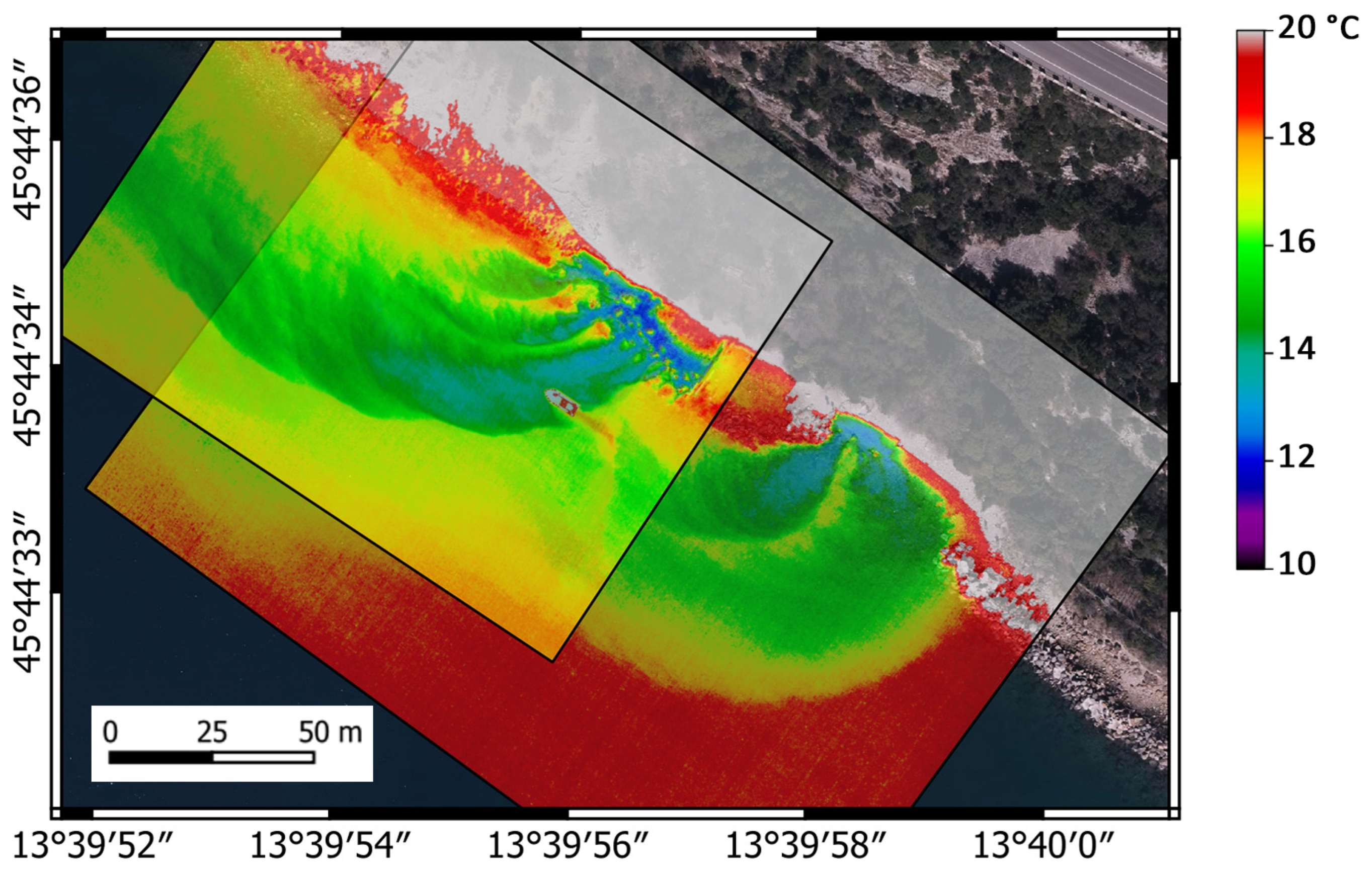
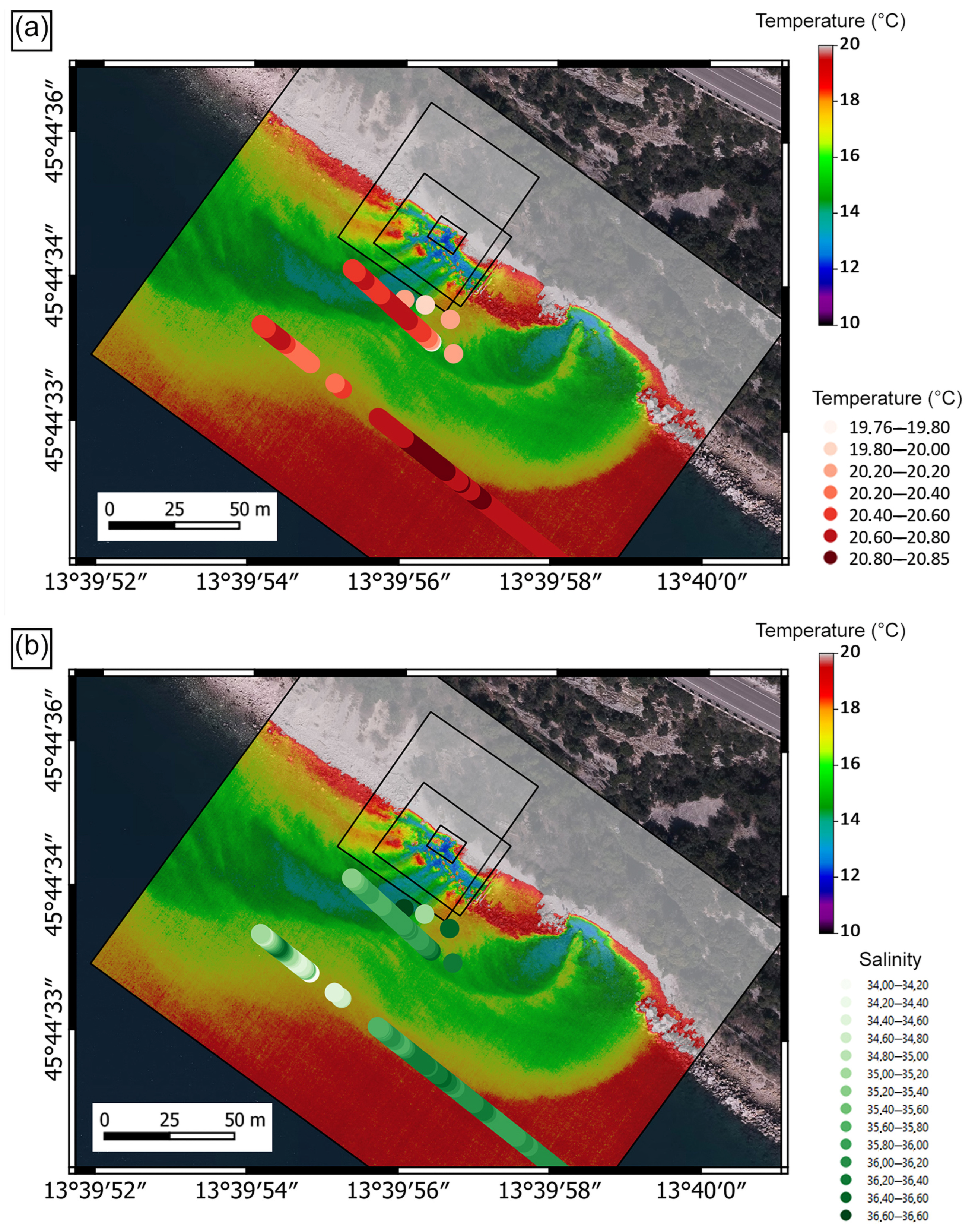
  • The drone proved to be able to clearly detect the thermal contrasts between seawater and freshwater, confirming its usability for detecting relative temperature differences between different water masses [8]. Anyway, attention must be paid when several drone images collected at different altitudes or times are merged together as the drone may assign different temperatures to the same surface, not following a precise trend due to light condition variations;
  • In case it is necessary to know the absolute values of sea surface temperature, it might be advisable to couple the drone survey with an oceanographic sampling on site (as we did), so as to correct the thermal values detected by the drone with real data. In particular, if the probe is equipped with sensors for variables other than temperature (like conductivity, chlorophyll concentration, turbidity, etc.), this procedure can provide additional data to support the findings. Particular care has to be taken to select the side of the boat that enters the water mass first, in order to avoid any possible perturbation of the surface water features due to the boat;
  • The heterogeneity of the surface under investigation or of cloud coverage could hamper an accurate correction of temperature values provided by drone imagery. Clearly, in emergency situations (such an oil spill or an accidental wastewater discharge), it may be impossible to wait for the ideal irradiation conditions, therefore this uncertainty factor must be taken into account.
  • To assemble the photo-mosaic, it is necessary to geo-reference the images. In general, the drone provides an accuracy on its positioning of approximately 2–4 m through aerial triangulation and onboard GNSS. To achieve better accuracy (up to a few cm), it is possible to apply other approaches. Natural GCPs extracted from true orthophotos can be used, and in this case the obtained resolution is that of the orthophoto. For this reason, it is advisable to capture images that contain part of the emerged land or fixed reference points at sea such as platforms and beacons. Otherwise, new GCPs, regularly distributed in the survey area, should be signalized and measured. However, the use and measurement of new GCPs is time-consuming and sometimes even not realizable [21]. As an alternative to the previous method, it is possible to use drones with an onboard multi-sensor system (e.g., dual-frequency GNSS chip, IMU, etc.) and RTK (Real Time Kinematics) or NRTK (Network Real Time Kinematic) GNSS technique, which provide precise information in real time with no need for GCPs [22]. However, the use of these techniques may encounter limitations caused by the presence of natural (e.g., cliffs) or artificial obstructions [23], unstable LTE signal or bad satellite configuration. The best resolution could be obtained by combining the use of GCPs and RTK/NRTK technique [24,25].

5. Conclusions

Oceanographic campaigns from ships and measurements with drones are two different, yet complementary, approaches.
Oceanographic campaigns are essential to understand the characteristics of water masses along the water column, but access to surface information is often complicated because it could be difficult to operate a probe on the water surface.
Drone surveys, on the other hand, cannot gather information underwater deeper than the sea surface, but they can quickly give an indication of the dynamics at the surface. Understanding these dynamics is sometimes crucial, as it allows, for example, immediate protective measures to be taken in the event of an accidental spill of contaminants, or to refine the design of a study along the water column in locations that could be of great interest, such as along fronts that also appear at the surface. In addition, access to certain study areas by sea is sometimes not possible, and the use of the drone makes it possible to obtain very valuable information that could not have been obtained using classical methods.
The combination of different methods and technologies in a multidisciplinary approach thus proves to be the most advisable method for investigating complex environments.

Author Contributions

Conceptualization, P.P., M.B., M.G. and R.G.; methodology, P.P., M.B. and R.G.; formal analysis, G.S., P.P., A.P. and R.G.; investigation, G.S., P.P., A.P., M.B., M.D.C., S.K. and R.G.; resources, P.P., A.P. and R.G.; data curation, G.S., P.P., A.P., M.D.C. and R.G.; writing—original draft preparation, G.S., P.P., A.P., M.B. and R.G.; writing—review and editing, G.S., P.P., A.P., M.B., M.G., M.D.C., C.C., S.K. and R.G.; visualization, G.S., A.P., M.D.C. and R.G.; supervision, R.G. All authors have read and agreed to the published version of the manuscript.

Funding

This research received no external funding.

Data Availability Statement

The data presented in this study are available on request from the corresponding author.

Acknowledgments

The authors acknowledge Matteo Bazzaro (OGS) for performing the measurements at the freshwater spring outlet, and the staff of the Marine Protected Area of Miramare who drove the boat and provided technical support during the oceanographic sampling. We also acknowledge the editor and the three anonymous reviewers for their constructive comments that helped us to improve the manuscript.

Conflicts of Interest

The authors declare no conflict of interest.

References

  1. Klemas, V.V. Coastal and Environmental Remote Sensing from Unmanned Aerial Vehicles: An Overview. J. Coast. Res. 2015, 31, 1260–1267. [Google Scholar] [CrossRef]
  2. The European Space Agency. Available online: https://www.esa.int/Applications/Observing_the_Earth/Copernicus/Sentinel-2_overview (accessed on 2 October 2023).
  3. NASA Landsat Science. Available online: https://landsat.gsfc.nasa.gov/satellites/landsat-8/ (accessed on 2 October 2023).
  4. Sedano-Cibrián, J.; Pérez-Álvarez, R.; de Luis-Ruiz, J.M.; Pereda-García, R.; Salas-Menocal, B.R. Thermal Water Prospection with UAV, Low-Cost Sensors and GIS. Application to the Case of La Hermida. Sensors 2022, 22, 6756. [Google Scholar] [CrossRef] [PubMed]
  5. Muchiri, N.; Kimathi, S. A review of applications and potential applications of UAV. In Proceedings of the 2016 Annual Conference on Sustainable Research and Innovation, Nairobi, Kenya, 4–6 May 2016. [Google Scholar]
  6. Lira, C.; Taborda, R. Advances in Applied Remote Sensing to Coastal Environments Using Free Satellite Imagery. In Remote Sensing and Modeling; Finkl, C., Makowski, C., Eds.; Springer: Cham, Switzerland, 2014; Volume 9, pp. 77–102. [Google Scholar] [CrossRef]
  7. Mangel, A.R.; Dawson, C.B.; Rey, D.M.; Briggs, M.A. Drone applications in hydrogeophysics: Recent examples and a vision for the future. Lead. Edge 2022, 41, 540–547. [Google Scholar] [CrossRef]
  8. Lee, E.; Yoon, H.; Hyun, S.P.; Burnett, W.C.; Koh, D.C.; Ha, K.; Kim, D.J.; Kim, Y.; Kang, K.M. Unmanned aerial vehicles (UAVs)-based thermal infrared (TIR) mapping, a novel approach to assess groundwater discharge into the coastal zone. Limnol. Oceanogr. Methods 2016, 14, 725–735. [Google Scholar] [CrossRef]
  9. Mallast, U.; Siebert, C. Combining continuous spatial and temporal scales for SGD investigations using UAV-based thermal infrared measurements. Hydrol. Earth Syst. Sci. 2019, 23, 1375–1392. [Google Scholar] [CrossRef]
  10. KarisAllen, J.J.; Mohammed, A.A.; Tamborski, J.J.; Jamieson, R.C.; Danielescu, S.; Kurylyk, B.L. Present and future thermal regimes of intertidal groundwater springs in a threatened coastal ecosystem. Hydrol. Earth Syst. Sci. 2022, 26, 4721–4740. [Google Scholar] [CrossRef]
  11. Accerboni, E.; Mosetti, F. Localizzazione dei deflussi d’acqua dolce in mare mediante un conduttometro elettrico superficiale a registrazione continua. Boll. Geofis. 1967, 9, 255–268. [Google Scholar]
  12. Cucchi, F.; Zini, L.; Calligaris, C. Le Acque del Carso Classico—Progetto Hydrokarst (The Water of the Classical Karst—Project HydroKarst); Edizioni Università di Trieste: Trieste, Italy, 2015; p. 179. [Google Scholar]
  13. Eagle-FVG. Sistema di Consultazione delle Banche Dati della Regione Autonoma Friuli-Venezia Giulia. Connected to the “IRDAT: Infrastruttura Regionale di Dati Ambientali e Territoriali per la Regione Autonoma Friuli Venezia Giulia”. Available online: https://eaglefvg.regione.fvg.it/ (accessed on 3 August 2023).
  14. ARSO. Geoportal of the Slovenian Environment Agency, Ministry of the Environment, Climate and Energy. Available online: https://gis.arso.gov.si (accessed on 3 August 2023).
  15. Flir Commercial Systems. Advanced Radiometry, Application Note; Flir Commercial Systems: Goleta, CA, USA, 2014; pp. 1–18. [Google Scholar]
  16. 3D FLOW. Available online: https://www.3dflow.net/3df-zephyr-photogrammetry-software/ (accessed on 2 October 2023).
  17. Oberle, F.K.J.; Prouty, N.G.; Swarzenski, P.W.; Storlazzi, C.D. High-resolution observations of submarine groundwater discharge reveal the fine spatial and temporal scales of nutrient exposure on a coral reef: Faga’alu, AS. Coral Reefs 2022, 41, 849–854. [Google Scholar] [CrossRef]
  18. Lega, M.; Ferrara, C.; Persechino, G.; Bishop, P. Remote sensing in environmental police investigations: Aerial platforms and an innovative application of thermography to detect several illegal activities. Environ. Monit. Assess. 2014, 186, 8291–8301. [Google Scholar] [CrossRef] [PubMed]
  19. Sancho Martínez, J.; Fernández, Y.B.; Leinster, P.; Casado, M.R. Combining Unmanned Aircraft Systems and Image Processing for Wastewater Treatment Plant Asset Inspection. Remote Sens. 2020, 12, 1461. [Google Scholar] [CrossRef]
  20. Mishra, V.; Avtar, R.; Prathiba, A.P.; Mishra, P.K.; Tiwari, A.; Sharma, S.K.; Singh, C.H.; Yadav, B.C.; Jain, K. Uncrewed Aerial Systems in Water Resource Management and Monitoring: A Review of Sensors, Applications, Software, and Issues. Adv. Civ. Eng. 2023, 2023, 3544724. [Google Scholar] [CrossRef]
  21. Li, X.Y. Principle, Method and Practice of IMU/DGPS Based Photogrammetry. Ph.D. Thesis, Information Engineering University, Zhengzhou, China, 2005. [Google Scholar]
  22. Fazeli, H.; Samadzadegan, F.; Dadrasjavan, F. Evaluating the potential of RTK-UAV for automatic point cloud generation in 3D rapid mapping. Int. Arch. Photogramm. Remote Sens. Spat. Inf. Sci. 2016, XLI-B6, 221–226. [Google Scholar] [CrossRef]
  23. Zimmermann, F.; Eling, C.; Klingbeil, L.; Kuhlmann, H. Precise positioning of UAVs–dealing with challenging RTK-GPS measurement conditions during automated UAV flights. ISPRS Ann. Photogramm. Remote Sens. Spat. Inf. Sci. 2017, IV-2/W3, 95–102. [Google Scholar] [CrossRef]
  24. Eling, C.; Wieland, M.; Hess, C.; Klingbeil, L.; Kuhlmann, H. Development and evaluation of a UAV based mapping system for remote sensing and surveying applications. Int. Arch. Photogramm. Remote Sens. Spat. Inf. Sci. 2015, XL-1/W4, 233–239. [Google Scholar] [CrossRef]
  25. Rabah, M.; Basiouny, M.; Ghanem, E.; Elhadary, A. Using RTK and VRS in direct geo-referencing of the UAV imagery. NRIAG J. Astron. Geophys. 2018, 7, 220–226. [Google Scholar] [CrossRef]
Figure 1. (a) Map of the Gulf of Trieste in the Northern Adriatic Sea, and (b) focus on the study site. (a) The general map shows the surface hydrography of the Friulian Plain and the area surrounding the Karst Plateau (from LIDAR RAFVG 2017–2020 [13] and from LIDAR D96TM [14]). The natural freshwater springs along the karstic coast and in the lower Friulian Plain, together with the karstic underground water flow (with direction), were compiled and synthesized from [12]. The orange rectangle represents the study area. (b) In this map, the orthophoto (modified from true orthophoto RAFVG 2017–2020 [13]) denotes the study area at the Aurisina Springs. The purple dots and the yellow lines represent the location where oceanographic in situ CTD point and transect measurements were performed, respectively. The area surveyed by the drone is shown by the green rectangle. Maps were compiled in ArcGIS® software by Esri, datum WGS84, projection UTM33.
Remotesensing 15 04864 g001
Figure 2. Images of the freshwater springs taken during the drone and oceanographic surveys. (a) The northernmost spring, where the water overflows from the artificial channel and fans out towards the sea, with the boat used in this study. (b) The southernmost spring, located at the sea level boundary and visible at low tide.
Remotesensing 15 04864 g002
Figure 3. (a) The drone used in the present study. (b) Schematic representation of the drone flight during thermal images acquisition at different altitudes.
Remotesensing 15 04864 g003
Figure 4. Thermal map resulting from the mosaicking of images acquired by the drone at 190 m altitude. The boat entering the plume at the northernmost Aurisina spring is also captured.
Remotesensing 15 04864 g004
Figure 5. Vertical profiles of (a) temperature; (b) salinity; (c) density (σ) recorded in P1–P6.
Remotesensing 15 04864 g005
Figure 6. Temperature–salinity diagram of the profiles P1–P6 (θ corresponds to potential temperature, σ to density). The black lines represent the isopycnals. The red line ideally indicates the data collected at the depth of ca. 1 m, while the green one at ca. 2.5 m depth.
Remotesensing 15 04864 g006
Figure 7. Temperature, salinity and density (σ) measured along the two transects: (a) T1 and (b) T2. Distance is calculated from the beginning of the transect, i.e., from the southeast. Please note that in (b) there are some empty spaces along the transect T2 because data with depth less than 45 cm and more than 55 cm were excluded.
Remotesensing 15 04864 g007
Figure 8. Surface data from the oceanographic survey (colored dots) superimposed on the mosaicking of the thermal maps deriving from the different drone hovering altitudes (black squares/rectangles): (a) temperature, (b) salinity.
Remotesensing 15 04864 g008
Table 1. Mean temperature, salinity and density (σ) ± standard deviation recorded in profiles from P1 to P6 in the layer at 50 cm ± 5 depth.
ProfileN. of PointsTemperature (°C)Salinityσ (kg/m3)
P1420.06 ± 0.1536.20 ± 0.2825.67 ± 0.17
P2120.06 ± 0.0036.46 ± 0.0025.86 ± 0.00
P3219.86 ± 0.0135.03 ± 0.0124.82 ± 0.00
P4320.15 ± 0.0736.60 ± 0.0225.95 ± 0.00
P5220.55 ± 0.0135.38 ± 0.0024.91 ± 0.00
P6220.48 ± 0.0035.20 ± 0.0724.79 ± 0.05
Disclaimer/Publisher’s Note: The statements, opinions and data contained in all publications are solely those of the individual author(s) and contributor(s) and not of MDPI and/or the editor(s). MDPI and/or the editor(s) disclaim responsibility for any injury to people or property resulting from any ideas, methods, instructions or products referred to in the content.

