Article

Enhancing Hyperspectral Anomaly Detection with a Novel Differential Network Approach for Precision and Robust Background Suppression

1
School of Physics, Xidian University, Xi’an 710071, China
2
School of Mathematics and Statistics, The University of Melbourne, Parkville, VIC 3010, Australia
3
School of Electronics and Information Engineering, Wuxi University, Wuxi 214105, China
4
Science and Technology on Complex System Control and Intelligent Agent Cooperation Laboratory, Beijing Mechano-Electronic Engineering Institute, Beijing 100074, China
*
Author to whom correspondence should be addressed.
Remote Sens. 2024, 16(3), 434; https://doi.org/10.3390/rs16030434
Submission received: 22 December 2023 / Revised: 17 January 2024 / Accepted: 18 January 2024 / Published: 23 January 2024
(This article belongs to the Special Issue Remote Sensing for Geology and Mapping)

Abstract

:
The existing deep-learning-based hyperspectral anomaly detection methods detect anomalies by reconstructing a clean background. However, these methods model the background of the hyperspectral image (HSI) through global features, neglecting local features. In complex background scenarios, these methods struggle to obtain accurate background priors for training constraints, thereby limiting the anomaly detection performance. To enhance the capability of the network in extracting local features and improve anomaly detection performance, a hyperspectral anomaly detection method based on differential network is proposed. First, we posit that anomalous pixels are challenging to be reconstructed through the features of surrounding pixels. A differential convolution method is introduced to extract local punctured neighborhood features in the HSI. The differential convolution contains two types of kernels with different receptive fields. These kernels are adopted to obtain the outer window features and inner window features. Second, to improve the feature extraction capability of the network, a local detail attention and a local Transformer attention are proposed. These attention modules enhance the inner window features. Third, the obtained inner window features are subtracted from the outer window features to derive differential features, which encapsulate local punctured neighborhood characteristics. The obtained differential features are employed to reconstruct the background of the HSI. Finally, the anomaly detection results are extracted from the difference between the input HSI and the reconstructed background of the HSI. In the proposed method, for each receptive field kernel, the optimization objective is to reconstruct the input HSI rather than the background HSI. This way circumvents problems where the background constraint biases might affect detection performance. The proposed method offers researchers a new and effective approach for applying deep learning in a local area to the field of hyperspectral anomaly detection. The experiments are conducted with multiple metrics on five real-world datasets. The proposed method outperforms eight state-of-the-art methods in both subjective and objective evaluations.

1. Introduction

Hyperspectral images (HSIs) are 3D image matrices captured by remote sensing imaging systems [1,2,3]. They encompass numerous narrow and approximately continuous spectral bands, covering the ultraviolet, visible, and infrared ranges [4,5,6]. The abundance of spectral information is advantageous for discriminating targets of interest with distinct spectral characteristics [7,8,9]. As a result, HSI has been applied in the field of target detection [10,11,12].
Hyperspectral anomaly detection refers to the unsupervised detection of targets that exhibit differences in both spatial and spectral characteristics from the surrounding background, without any prior information [13,14]. This technique has been applied in different areas, such as environmental monitoring, resource exploration, and precision agriculture [15,16]. Despite the unique advantages of hyperspectral anomaly detection, it faces various challenges, including the absence of prior information, diverse background types, and noise interference [17,18].
In past decades, plenty of hyperspectral anomaly detection methods have emerged to solve various problems. The existing hyperspectral anomaly detection methods can be categorized into traditional methods and deep-learning-based methods [19,20]. The traditional methods can be further classified into statistical-based methods and data-representation-based methods [21,22]. The statistical-based methods aim to model the background distribution of the HSI and identify target locations through hypothesis testing [23,24]. In the statistical-based methods, the Reed–Xiaoli (RX) method [25] is recognized as one of the most representative methods. This method assumes that the background of HSI obeys a multivariate Gaussian distribution. The anomalous targets are detected by calculating the Mahalanobis distance between the test pixels and the background. However, in the real HSI, the mean and covariance used by the RX method are susceptible to interference from anomalies and noise when the background information is complex. This will impact detection performance. To reduce the impact of anomalies and noise on detection results, methods like local RX [26] and kernel RX [27,28] are proposed. To precisely model complex backgrounds in situations with multipixel anomalies, the two-step generalized likelihood ratio test (2S-GLRT) [29] has been introduced. This method is a generalization of the RX method. It employs Gaussian hypothesis testing to detect anomalous targets by modeling multipixel anomalies and background. Data-representation-based methods posit that background pixels can be reconstructed by some similar background pixels [30]. Among them, the collaborative representation detector (CRD) [31] assumes that each background pixel can be approximated by other pixels in its spatial neighborhood while anomalous pixels cannot. This method uses background reconstruction errors to extract anomalies. Detectors based on low-rank sparse representation [32,33] consider that the background is low-rank and anomalies are sparse. These methods achieve low-rank and sparse representation through the constructed background dictionary. For instance, Zhang et al. [34] propose a hyperspectral anomaly detection method based on low-rank sparse matrix decomposition and Mahalanobis distance. This method utilizes the constructed background dictionary for low-rank and sparse decomposition and employs Mahalanobis distance for anomaly detection. Wang et al. [35] introduce a hyperspectral anomaly detection method based on principal component analysis and tensor low-rank and sparse representation (PCA-TLRSR). In this method, a vector low-rank and sparse representation method is used instead of the traditional 2D representation to preserve the 3D information of the HSI. A comprehensive 3D background dictionary is constructed for low-rank and sparse representation. The traditional methods have been successfully applied in practical applications due to the efficient execution [36]. However, for complex HSI scenarios, statistical-based methods struggle to acquire accurate background statistical features, which may affect detection performance. The data-representation-based methods face challenges in establishing precise background dictionaries, which reduces the accuracy of the obtained low-rank and sparse matrices.
Deep-learning-based methods can extract latent deep features from the HSI to achieve precise mapping of complex scenes through outstanding nonlinear fitting capabilities. The deep-learning-based methods can be categorized into supervised methods and unsupervised methods depending on the availability of labels [37,38]. The supervised methods train classifiers under a plethora of labels to facilitate anomaly detection. However, due to the absence of ground truth labels, these methods use other methods to generate pseudo-labels [39]. For instance, Li et al. [40] utilize reference data with labels to train a convolutional neural network (CNN), extracting differentiating features between spectra. Then, the trained CNN is employed for anomaly detection. Rao et al. [41] propose a hyperspectral anomaly detection method based on a Siamese Transformer network. This method utilizes a small set of prior spectral signatures and spectral unmixing to construct pseudo-labels for training data. The Siamese network is then optimized for anomaly target detection. The unsupervised methods extract deep features from the HSI in the absence of labels. Currently, generative models have been applied in the field of hyperspectral anomaly detection [38]. For example, Xiang et al. [42] introduce a method based on a guided autoencoder network (GAED). This method acquires the guided image through the spectral similarity. Then, the guided image is used to guide the training process of the autoencoder. An anomaly detection result is obtained from the reconstruction error. Wang et al. [43] propose an anomaly detection method based on the autonomous anomaly detection network (Auto-AD). The Auto-AD method reconstructed the background of the HSI by training on random noise and utilized residuals for anomaly detection. Jiang et al. [44] introduce a low-rank embedded network (LREN). In this method, a low-rank prior is introduced into the autoencoder network to guide the network optimization towards the lowest rank for background reconstruction. The anomaly detection result is extracted from the residual image. Fu et al. [45] present a plug-and-play denoising regularization anomaly detection method named DeCNNAD. This method introduces an effective CNN denoiser into low-rank representations to reconstruct a clean background. The above deep-learning-based methods globally model the HSI background as low-rank [8]. These methods have yielded satisfactory results. However, these methods overlook the local features around the anomalies, which are important features in hyperspectral anomaly detection. Training only with global constraints makes it difficult to acquire a clean reconstructed background. This limitation constrains the effectiveness of these methods in anomaly detection.
As analyzed above, the detection performance of the existing traditional methods is limited by the finite feature descriptors and imprecise background statistical models. Moreover, deep-learning-based methods are susceptible to neglecting the surrounding local features of anomalies, which can lead to overfitting of the training. The reconstructed background is then interfered with by anomalies. To solve these problems, motivated by the CRD [31], a local prior is introduced into the deep leaning method. We extend the assumption of the CRD from pixels to features. We posit that anomalous features in HSI are difficult to be represented by local features in the surrounding neighborhoods. So, the neighborhood features make it easy to reconstruct a clean background. To extract the local punctured features, a hyperspectral anomaly detection method based on differential network is proposed. In the differential network, a novel differential convolution is designed through the difference among two types of kernels. For each type of kernel, the objective is to reconstruct the input HSI instead of the background HSI. Background HSI is estimated through the difference operation. This way avoids the problem that the reconstructed background HSI receives interference from anomalies. Specifically, in the proposed method, first, 5 × 5 and 3 × 3 convolutional kernels are employed to extract outer window features and inner window features, respectively. Second, to enhance the expression capability of internal window features for details and crucial information, outer window features are utilized to guide inner window features, and two local guidance attention modules are proposed. Among them, local detail attention strengthens the ability of inner window features to extract edge details, while local Transformer attention enhances the focus ability of inner window features on salient information. Third, the obtained inner window features are subtracted from the outer window features to derive differential features. These differential features can be used to reconstruct a clean background of the HSI. Fourth, by concatenating all differential features along the channel dimension and applying a 1 × 1 convolution for feature fusion, the reconstructed background HSI is obtained. Finally, the anomaly detection result is derived from the residuals between the input HSI and the reconstructed background HSI.
The main contributions of this work are as follows:
(1)
A differential convolutional network is proposed to extract the local punctured neighborhood features for background reconstruction.
(2)
To enhance the capability of the network to extract details, a local detail attention module is proposed.
(3)
To enhance the focusing ability of the network on important features, a local Transformer attention module is proposed.
This paper is organized as follows. In Section 2, the proposed method is introduced in detail. In Section 3, the experimental details and results are shown, and the effectiveness of the proposed method is discussed. In Section 4, we conclude this paper.

2. Proposed Method

The framework of the proposed method is shown in Figure 1. The 5 × 5 and 3 × 3 convolution are used to extract outer window features and inner window features. The proposed local detail attention and local Transformer attention are added to the network for enhancing the inner window features. The differential features are obtained by the difference between the outer window features and inner window features. All the differential features are concatenated and fused to obtain the background HSI. The anomaly detection result is obtained through the residual of the input HSI and background HSI.
In the following sections, we first describe the differential convolutional neural network in detail in Section 2.1. Then, to improve the feature representation capabilities, two local guidance attention modules named local detail attention and local Transformer attention are introduced in Section 2.2 and Section 2.3. In Section 2.4, the training loss of the proposed method is described. In Section 2.5, the network prediction and anomaly target extraction are explicated.

2.1. Differential Convolutional Neural Network

Recently, many anomaly detection methods based on CNNs and autoencoders have been proposed to obtain satisfactory results. These methods reconstruct a clean background and subsequently detect anomalies from residual images. CNN-based methods utilize simple convolutional kernels to extract the spatial–spectral features of the target. The global low-rank constraints are adopted during network training. However, local features around the anomalies are ignored. As training progresses, there is a possibility that the network indiscriminately learns anomalous features, resulting in the contamination of reconstruction background by anomalies. As such, this training process is uncontrollable. On the other hand, the methods based on autoencoders usually employ autoencoder networks for spectral reconstruction and add spatial features through other strategies. This, to some extent, severs the spatial–spectral relationship in the HSI. To further exploit the local features of anomalies, inspired by CRD, an anomaly detection method based on a differential convolutional neural network (DifferNet) is proposed.
We represent the input HSI as Y = ( y 1 , y 2 , , y M · N ) R M × N × B , where M and N denote the spatial dimensions of the HSI, and B represents the spectral dimension. In the input HSI, background pixels can be represented by other pixels within their local neighborhood, while anomalous pixels cannot. Thus, in a local window, the objective function can be expressed as
arg min θ y i f ( X s ( y i ) ; θ ) 2 2 + α θ 2 2 , i = 1 , 2 , , M · N
where X s ( y i ) represents the set of local punctured neighborhood of pixel y i , and X s is the set of local punctured neighborhoods at all the pixels. θ denotes the network parameters to be optimized, f ( · ) is the mapping function from network input to output, and α is the regularization parameter.
To extract the local punctured neighborhood pixels of the pixel to be tested, a differential convolution method is proposed. The general form of the proposed convolution can be expressed
F = w X s + b
where w is the convolution weights defined on the set X s , b is the bias defined on the set X s , ⊛ denotes the convolution operation, and F denotes the convolution output feature. X s can be represented as
X s = X o u t X i n
where X o u t and X i n are the sets of pixels in the local outer window and local inner window centered by pixel y i , respectively. ⊖ denotes the set difference operation. It is worth noting that the convolution weights w and bias b operate on the punctured neighborhood. Therefore, their values are zero on the local inner window X i n . Thus, Equation (2) can be expressed as
F = w ( X o u t X i n ) + b = w o u t X o u t w i n X i n + b = F F
w = w o u t w i n
F = w o u t X o u t + b o u t
F = w i n X i n + b i n
where w o u t and w i n represent the weights of the convolution defined on X o u t and X i n , respectively. The weights w o u t and w i n have the same values on set X i n . Similarly, b o u t and b i n denote the biases of the convolution defined on X o u t and X i n , respectively. Biases b o u t and b i n have the same values on set X i n . F and F represent the convolution output features on X o u t and X i n , respectively.
Equation (4) indicates that we can obtain the estimated feature of the test pixel y i in the local punctured neighborhood X s by taking the difference of convolution features with different receptive field sizes. To implement such convolution operations, the most direct approach is to extract smaller convolution kernels within a larger receptive field. However, this approach completely neglects inner window pixels in the convolution operation, potentially introducing artificial biases in the results. Therefore, we relax the constraints on convolution kernels w o u t and w i n , allowing for different weights and biases on the set X i n . Correspondingly, to enhance the effectiveness of the difference, learnable weighting parameters λ are introduced to the differential operation. Thus, the proposed differential convolution can be expressed as
g ( X o u t , X i n ) = F λ × F = w o u t X o u t + b o u t λ × ( w i n X i n + b i n )
Specifically, the proposed DifferNet is structured as illustrated in Figure 1. We employ convolution kernels of sizes 5 × 5 and 3 × 3 to construct the differential convolution. For the j-th layer, with the outer window input features F o u t j 1 and the inner window input features F i n j 1 , the differential convolution produces three output features, including outer window output feature F o u t j , inner window output feature F i n j , and differential output feature F d i f j . This process can be represented as
Z o u t j = w o u t j F o u t j 1 + b o u t j , j = 1 , 2 , .
F o u t j = max α s l o p e × Z o u t j , Z o u t j , j = 1 , 2 , .
Z i n j = w i n j F i n j 1 + b i n j , j = 1 , 2 , .
F i n j = max α s l o p e × Z i n j , Z i n j , j = 1 , 2 , .
F d i f j = F o u t j λ j × F i n j , j = 1 , 2 , .
where w o u t j and b o u t j represent the weights and biases of the j-th 5 × 5 convolutional layer, respectively. Similarly, w i n j and b i n j denote the weights and biases of the j-th 3 × 3 convolutional layer, respectively. Z o u t j and Z i n j are the outputs of the 5 × 5 convolutional layer and the 3 × 3 convolutional layer, respectively. λ j is the weighting coefficient for the j-th differential convolutional layer. Following each convolutional layer, the activation function is the LeakyReLU function, as shown in Equation (10), where α s l o p e is the slope of the negative axis. The input features F o u t 0 and F i n 0 are derived from the input HSI Y . The outer window output feature and inner window output feature at the final level contribute to the reconstruction of the HSI.
After all the differential features are obtained, they are concatenated along the channel dimension to obtain the combined differential feature F c o m b i n e . Subsequently, a 1 × 1 convolutional layer and LeakyReLU activation are employed to fuse all differential features. The predicted background HSI B is obtained. This process can be described as
F c o m b i n e = f C o n c a t ( F d i f 1 , F d i f 2 , F d i f 3 , F d i f 4 )
B = f L e a k y R e L U ( f C o n v ( F c o m b i n e ) )
where f C o n c a t ( · ) denotes the channel concatenation operation, f C o n v ( · ) represents the 1 × 1 convolution operation, and f L e a k y R e L U ( · ) is the LeakyReLU activation function.
Due to the differences in receptive fields in the proposed differential convolution, the 5 × 5 branch and the 3 × 3 branch exhibit variations in their reconstructive capabilities for HSI. Compared to the 3 × 3 convolutional layer, the 5 × 5 convolutional layer can capture information over a broader range, leading to better perception and localization of edge details. Therefore, to enhance the expressive capability of the 3 × 3 convolutional layer, we propose two guidance attention modules, namely the local detail attention (LDA) and the local Transformer attention (LTA). These modules leverage the features from the 5 × 5 convolutional layer to guide the features of the 3 × 3 convolutional layer. Then, the finely detailed fusion features can be obtained. In the following two sections, we will provide a detailed explanation of these two guidance attention modules.

2.2. Local Detail Attention

The proposed structure of differential network successfully divides the traditional background reconstruction into two steps: comprehensive feature representation of input HSI and background features extraction through difference operation. During the feature representation step, the more comprehensive the features extracted by convolutional networks, the more beneficial it is for reconstructing the background. To enhance the capability of network to extract details and acquire comprehensive feature representations of the input HSI, a local detail attention is designed. Traditional convolutional operations typically utilize the same convolution kernel across the entire image. However, this convolutional approach lacks adaptive handling of variations in local details, resulting in a degree of information loss. To effectively capture local details in the HSI, inspired by the work [46], a local detail attention module is proposed.
The proposed local detail attention module is illustrated in Figure 2. Given the input inner window feature F i n R M × N × C and the input outer window feature F o u t R M × N × C , where C is the number of feature channels, the local detail attention learns a set of base convolutional kernels W = { W i | i = 1 , 2 , , n b a s e } R n b a s e × C × c g r o u p × k × k from the input outer window features F o u t . These base convolutional kernels are associated with fusion coefficients at different positions in the image. Utilizing these base convolutional kernels and fusion coefficients, a fused convolutional kernel is calculated and applied to the image for convolution. Then, the detail attention features are obtained. The obtained detail attention features are added to the input inner window feature F i n , yielding the output inner window feature F i n d a . F i n d a is used to replace F i n as the input for the next-level differential convolution, introducing more detail attention into the inner window features.
The base convolutional kernels W consist of n b a s e group convolution kernels, each with a size of C × c g r o u p × k × k . c g r o u p represents the number of channels per group in group convolution, and the number of groups is C c g r o u p . k denotes the spatial dimension of the convolutional kernel. The group convolution can balance the efficiency and effectiveness of the module.
Specifically, first, to obtain the fusion coefficients for the base convolutional kernels, a fusion attention module is introduced. This module integrates local information through a 3 × 3 convolution. Subsequently, a SimpleGate activation function [47] is employed for further feature transformation. Following that, a 1 × 1 convolution is used for feature fusion and channel mapping to n b a s e . A residual connection containing a 1 × 1 convolution is utilized to supplement additional detail features.
Second, after the fusion attention module, the fusion coefficient map D R M × N × n b a s e are obtained. Combining with the base convolutional kernels W , the fused convolutional kernel K ( i , j ) R C × c g r o u p × k × k at position ( i , j ) can be calculated by
K ( i , j ) = t = 1 n b a s e ( D ( i , j , t ) × W t )
where W t R C × c g r o u p × k × k represents the t-th convolutional kernel in the base convolutional kernels W , and D ( i , j , t ) denotes the t-th fusion coefficient at position ( i , j ) in the fusion coefficient map D.
Third, the obtained fused convolutional kernel K ( i , j ) is utilized to compute the feature F D A ( i , j ) R 1 × C at position ( i , j ) in the detail attention feature F D A R M × N × C .
F D A ( i , j ) = f G r o u p C o n v ( F o u t ( i , j ) , K ( i , j ) )
where f G r o u p C o n v ( · ) denotes the group convolution operation, and F o u t ( i , j ) represents the features in the receptive field at position ( i , j ) in the input outer window feature F o u t .
Finally, the obtained detail attention features F D A are weighted summed with the input inner window feature F i n to obtain the output inner window feature F i n d a .
F i n d a = F i n + γ F × F D A
where γ F represents the learnable weighting parameter. The resulting F i n d a is used to replace F i n as the input for the next-level differential convolution.
The pseudo-code table for the proposed local detail attention is shown in Algorithm 1.
Algorithm 1 Pseudo-code of the proposed local detail attention.
   Input:
       F o u t , input outer window feature with shape [1, C, M, N]
       F i n , input inner window feature with shape [1, C, M, N]
   Output: F i n d a , output inner window feature with shape [1, C, M, N]
   Hyperparameters: n b a s e the number of base convolutional kernels
   Operators:
      FA, fusion attention model
      Conv, Convolution
   Fusion coefficients C = FA( F o u t ) with shape [1, n b a s e , M, N]
   for i = 1 to M
      for j = 1 to N
         W = zeros([1, C, 5, 5])
         for k = 1 to n b a s e  do
            W = W + C[i, j, k] × W[K]
         end for
          F D A [i, j, :] = Conv( F o u t [i − 2:i + 2, j − 2:j + 2, :], W)
      end for
   end for
    F i n d a = F i n + γ F × F D A

2.3. Local Transformer Attention

In recent years, Transformer module [48,49,50] has gained widespread attention and research due to its outstanding performance. It is a global attention module capable of establishing long-range dependencies across images, exhibiting strong feature extraction capabilities. However, the computation of attention weights in Transformer involves matrix multiplication over global pixels, resulting in significant computational and memory requirements. This hinders its application in hyperspectral anomaly detection. Considering that anomalous targets in hyperspectral anomaly detection typically occupy a few pixels in spatial dimension, the establishment of global dependencies for feature extraction is unnecessary. Compared to global information, nonlocal information is more useful for anomaly detection. Therefore, to focus on nonlocal essential information, we modify the way of calculating the attention coefficients and propose a local Transformer attention (LTA) module. Through the LTA model, the network is capable of focusing on salient regions in the scene, enhancing its ability to represent features in the input HSI. This contributes to the comprehensiveness of feature representation, promoting the reconstruction of background HSI.
The proposed local Transformer attention module is illustrated in Figure 3. First, given the input inner window feature F i n R M × N × C and input outer window feature F o u t R M × N × C , a query map Q R M × N × C is obtained by performing a 1 × 1 convolution on F o u t . Second, two convolutional layers are employed to approximate the matrix multiplication in Transformer, yielding the correlation map F q v R M × N × r 2 . Here, an r × r convolutional layer is used to capture the nonlocal receptive field and map the feature channels to r 2 , where r denotes the spatial size of the nonlocal receptive field. The LeakyReLU function enhances the nonlinear representation capacity. Then, a 1 × 1 convolutional layer are employed to merge channel features, establishing the correlation of attention coefficients within the receptive field. Third, the correlation coefficients F q v ( i , j ) at position ( i , j ) is extracted and reshaped into r × r . Fourth, the Transformer attention feature F T A R M × N × C at position ( i , j ) can be calculated by
F T A ( i , j ) = S o f t m a x ( F q v ( i , j ) ) F o u t r ( i , j )
where F o u t r ( i , j ) represents the nonlocal region of size r within F o u t at position ( i , j ) .
Fifth, the obtained Transformer attention feature is concatenated with F i n along the channel dimension. Then, the integrated feature F t a c is obtained. It can be represented by
F t a c = f C o n c a t ( F i n , F T A )
Finally, through a 1 × 1 convolutional layer for feature fusion, the output inner window feature F i n t a R M × N × C is obtained. The F i n t a is used to replace F i n as the input for the next-level differential convolution.
The pseudo-code table for the proposed local Transformer attention is shown in Algorithm 2.
Algorithm 2 Pseudo-code of the proposed local Transformer attention.
   Input:
       F o u t , input outer window feature with shape [1, C, M, N]
       F i n , input inner window feature with shape [1, C, M, N]
   Output: F i n t a , output inner window feature with shape [1, C, M, N]
   Hyperparameters: c g r o u p the number of group channels
   Operators:
      Conv(F, r), feature convolution on feature F with kernels size r
      act, Leaky ReLU activation   Cat, Concatenation
   Generate query map Q = Conv( F o u t , 1) with output shape [1, C, M, N]
   Extract nonlocal features F n l = act(Conv(Q, r)) with output shape [1, r 2 , M, N]
   Map to coefficients F q v = Conv( F n l , 1) with output shape [1, r 2 , M, N]
   for i = 1 to M
      for j = 1 to N
          F T A [i, j, :] = F o u t [i−r:i+r, j−r:j+r, :]·Softmax( F q v [i, j, :])
      end for
   end for
    F t a c = Cat( F i n , F T A )
    F i n t a = Conv( F t a c , 1)

2.4. Loss Function

In the proposed DifferNet, it is imperative to fully explore features in the HSI, encompassing both anomalous and background features. This approach differs from the existing CNN-based methods, which focus on extracting background features while ignoring anomalous features. The proposed method avoids the problem of background contamination caused by anomalies in traditional networks.
For the outputs of the 5 × 5 branch Y 1 R M × N × B and the 3 × 3 branch Y 2 R M × N × B , the loss function is defined as follows
L r e c o n s t r u c t = S m o o t h L 1 ( Y 1 , Y ) + S m o o t h L 1 ( Y 2 , Y )
where S m o o t h L 1 ( · ) is the smooth L1 function [51]. It is calculated by
f S m o o t h L 1 ( x , y ) = 0.5 ( x y ) 2 , | x y | < 1 | x y | 0.5 , | x y | > 1
For the predicted background HSI B of the differential network, as anomalies occupy a small portion in the HSI, we choose the input HSI Y as the optimization target in consideration of computational efficiency. The loss function of the background is formulated as
L b a c k g r o u n d = S m o o t h L 1 ( B , Y )
Therefore, the total loss function is
L = 1 2 ( L r e c o n s t r u c t + L b a c k g r o u n d )

2.5. Anomaly Target Extraction

After the training completion of the proposed DifferNet, the HSI Y is fed into the network to obtain the predicted background HSI B = ( b 1 , b 2 , , b M · N ) . The difference between the input HSI and the predicted background HSI is calculated to obtain the anomaly detection result. The anomaly detection result E can be represented as
E i = j = 1 B ( | y i ( j ) b i ( j ) | ) B T ξ , i = 1 , 2 , , M · N
where y i ( j ) is the j-th element of the input pixel y i , b i ( j ) is the j-th element of the predicted background pixel b i , and E i represents the value of the anomaly detection result E at position i, ξ is the detection threshold to separate the targets T from the background B .
The pseudo-code table for the proposed method is shown in Algorithm 3.
Algorithm 3 Pseudo-code of the proposed method.
   Input: Y, hyperspectral image with shape [1, B, M, N]
   Output: E, anomaly detection result
   Hyperparameters:
       n b a s e the number of base convolutional kernels
       c g r o u p , the number of group channels
       p l d , the position of local detail attention
       p l t , the position of local Transformer attention
       l r , learning rate
       β m a x , maximum training epochs
       β s t e p , the number of epochs at which learning rate decays
       σ d e c a y , factor by which learning rate decays
   Operators:
      DN, differential network with local detail attention and local Transformer attention
      L, Loss function
      norm1, Vector L1 norm
   Construct the network using parameters n b a s e , c g r o u p , p l d , and p l t .
   for i = 1 to β m a x  do
         Predicting process [ Y 1 , Y 2 , Y d i f f e r ] = DN(Y)
         Total loss is calculated by t l o s s = L( Y 1 , Y 2 , Y d i f f e r ;Y)
         Weight gradients of back propagation G = t l o s s W
         if i mod  β s t e p is 0 do
                l r = σ d e c a y × l r
         end if
         Weights update by W = W − l r × G
   end for
   Background prediction [_, _, B]=DN(Y)
   Anomaly detection E = norm1(YB, dim=1)

3. Results and Disscussion

In this section, different experiments are conducted to prove the superiority of the proposed method. In the experiments, we use eight state-of-the-art methods as comparison methods. The comparison methods include the RX [25], the CRD [31], the 2S-GLRT [29], the PCA-TLRSR [35], the GAED [42], the Auto-AD [43], the LREN [44], and the DeCNNAD [45] methods. Firstly, we introduce the experimental datasets and the evaluation metrics. Then, the parameters of the proposed method and the comparison methods are analyzed. Next, the experimental results of different methods are performed on five real-world datasets. Finally, the structural effectiveness and the module effectiveness are discussed.

3.1. Experimental Datasets

(1)
Bay Champagne: This dataset was collected at Bay Champagne, France, by the Airborne Visible/Infrared Imaging Spectrometer (AVIRIS) sensor [52] on 4 July 2010. This HSI is 100 × 100 in size with spatial resolution of 4.4 m, as shown in Figure 4a. The HSI data have 188 bands. All the bands are used in the experiments. The ship in the scene is regarded as an anomaly target.
(2)
Pavia: This dataset was collected at Pavia, Italy, by Reflective Optics System Imaging Spectrometer (ROSIS-03) sensor [52]. This HSI is 150 × 150 in size with spatial resolution of 1.3 m, as shown in Figure 4b. The HSI has 102 bands. The cars on the bridge are treated as anomaly targets.
(3)
SpecTIR: This dataset was obtained from the SpecTIR hyperspectral aircraft Rochester experiment [53]. This HSI is 180 × 180 in size with spatial resolution of 1 m and 120 in bands with spectral resolution of 5 nm. In the experiments, we select a 100 × 100 area with 120 bands as the experimental dataset, as shown in Figure 4c. The artificial-colored square fabrics are regarded as the anomaly targets.
(4)
WHU-Hi-River: This dataset was collected at a long river bank in Honghu, Hubei Province of China on 21 March 2018 [54]. This HSI is 105 × 168 in size with spatial resolution of 6 cm, as shown in Figure 4d. The HSI has 135 bands ranging from 0.4 μ m to 1 μ m. Two plastic plates and two gray panels are treated as anomaly targets.
(5)
MUUFLGulfport: This dataset was collected at University of Southern Mississippi Gulf Park Campus, Long Beach, Mississippi, in November 2010 [55,56]. This HSI is 325 × 220 in size and 72 in bands with 10 nm spectral resolution ranging from 375 nm to 1050 nm, as shown in Figure 5. In the experiments, 64 bands are selected by removing the noise bands. Four cloth panels in the scene are regarded as anomaly targets.

3.2. Evaluation Metrics

In the experiments, three evaluation metrics are adopted, including three-dimensional receiver operating characteristic curve (3D ROC) [57], two-dimensional ROC curve (2D ROC), and area under the 2D ROC curve (AUC). The 3D ROC curve can illustrate the relationships between the probability of detection ( P D ), the probability of false alarm ( P F ), and the threshold ( τ ). The 3D ROC can be decomposed into three 2D curves: ( P D , P F ), ( P D , τ ), and ( P F , τ ). They can show the detection performance and evaluate separation between anomalies and the background. The AUC values of these three 2D curves are donated by A U C ( D , F ) , A U C ( D , τ ) , and A U C ( F , τ ) , respectively. The A U C ( D , F ) is used to evaluate the overall performance of the detectors. The A U C ( D , τ ) is used to evaluate the target detection performance of detectors. The A U C ( F , τ ) is used to evaluate the background suppression performance of detectors. The larger the A U C ( D , F ) and A U C ( D , τ ) , the better the performance. The smaller the value of A U C ( F , τ ) , the better the performance.

3.3. Parameter Analysis and Experimental Setup

In this section, the experimental parameters of the proposed method and the comparison methods are performed. The parameters of the eight state-of-the-art comparison methods are set according to the suggestions of the authors or the performance in the A U C ( D , F ) . Specifically, in the RX method, there are no additional parameters that need to be set. In the CRD method, the sizes of the double window ( w o u t , w i n ) are set to (7, 5), (7, 5), (25, 21), (9, 5), and (17, 5) on the five datasets of Bay Champagne, Pavia, MUUFLGulfport, SpecTIR, and WHU-Hi-River, respectively. In the 2S-GLRT method, the double window sizes are set to (17, 15), (21, 5), (25, 21), (9, 5), and (11, 7) on the five datasets. In the PCA-TLRSR method, the numbers of principle components are set to 15, 9, 17, 11, and 13 on the five datasets. In the GAED method, the weights and bias are randomly initialized. As suggested by the authors, on all five datasets, the window size c is set to 7, the learning rate l a is set to 0.4, the penalty coefficient β is set to 1, the number of iterations is set to 300, and the dimension of the hidden layer is set to 25. In the Auto-AD methods, there are no uncertain parameters that need to be set. In the LREN method, the weights and bias are randomly initialized. The number of clusters and the size of hidden layer are set to 7 and 9 on all the datasets as suggested. The regularization parameters are set to 0.01, 0.01, 0.01, 1.0, and 1.0 on the five datasets, respectively. In the DeCNNAD method, the number of clusters is set to 9, 8, 8, 13, and 6 on the five datasets, respectively. The regularization parameters ( β , λ ) are set to (0.01, 0.01), (0.01, 0.01), (0.0001, 0.0001), (0.001, 0.01), and (0.01, 0.01) on the five datasets, respectively.
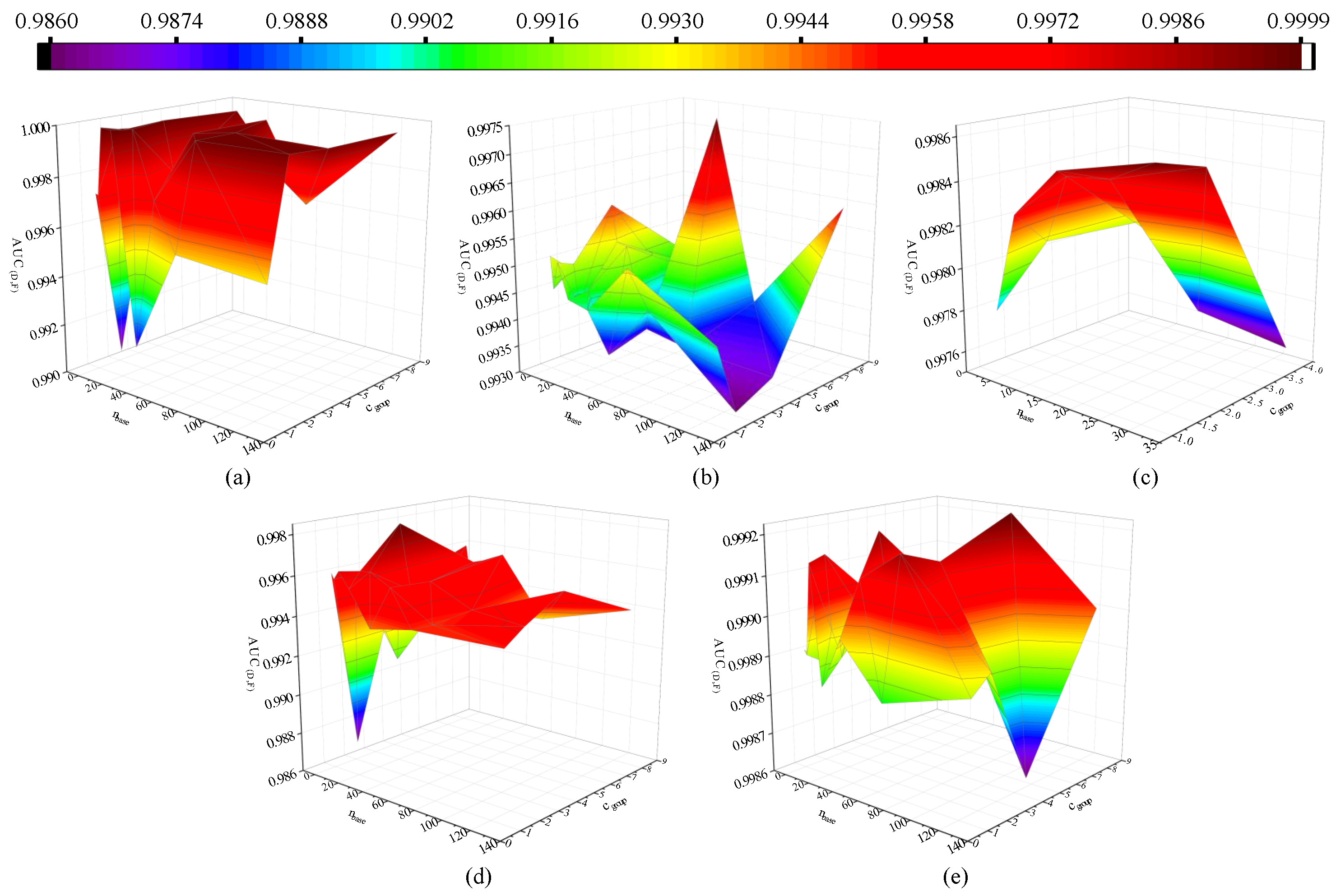
For the proposed method, before our experiments, the datasets are first normalized. The weights and bias are randomly initialized. The hyperparameters include learning rate l r , maximum training epochs β m a x , the number of epochs at which learning rate decays β s t e p , and the factor by which learning rate decays σ d e c a y . In our experiments, on all five datasets, l r = 0.001 , β m a x = 4000 , β s t e p = 1000 , σ d e c a y = 0.5 . The uncertain parameters include the number of base convolutional kernels n b a s e and the number of group channels in the group convolution c g r o u p . In addition, the position of the local detail attention and local Transformer attention also influence the performance of the proposed method. Hence, we analyze the positions p l d and p l t of these two modules, where p l d represents the position of the local detail attention and p l t represents the position of the local Transformer attention. To analyze the stability of these parameters, some parameters are conducted by varying the parameters. Because the weights and bias are randomly initialized, the performance of different experiments will randomly change. So, to reduce the influence of random initialization, we fix the random seed on different datasets during the parameter analysis experiments. This ensures that the performance of the proposed method with different parameters is comparable.
We vary the value of the n b a s e in 2, 4, 8, 16, 32, 64, and 128. The value of the parameter c g r o u p is varied in 1, 2, 4, and 8. The optimal results of the n b a s e and c g r o u p are shown in Figure 6. To constrain the size of the network, only one module is adopted for both the local detail attention and the local Transformer attention. We vary the values of the p l d and p l t in 1, 2, 3, which means that the position is after the first, second, or third convolution layer in the network, respectively. The optimal results of the p l d and p l t are shown in Figure 7.
As shown in Figure 6, the performance on the datasets of MUUFLGulfport and WHU-Hi-River is stable while changing the n b a s e and c g r o u p . The A U C D , F are concentrated above 0.9976 on these two datasets. The range of the A U C D , F is about 0.0008 and 0.0006 on the datasets of MUUFLGulfport and WHU-Hi-River, respectively. On the datasets of Bay Champagne, Pavia, and WHU-Hi-River, the performance is unstable while changing the n b a s e and c g r o u p . The range of the A U C D , F is 0.0094, 0.0042, and 0.0110 on these three datasets, respectively. However, most A U C D , F values of these three datasets are concentrated above 009935. According to the A U C D , F performance, the parameters ( n b a s e , c g r o u p ) are set to (8, 1), (32, 8), (32, 1), (8, 4), and (64, 8) on the datasets of Bay Champagne, Pavia, MUUFLGulfport, SpecTIR, and WHU-Hi-River, respectively.
As shown in Figure 7, the performance on the five datasets is stable while changing the p l d and p l t . The A U C D , F are concentrated above 0.9930. The range of the A U C D , F is 0.0027, 0.0038, 0.0008, 0.0048, and 0.0096 on the five datasets, respectively. According to the A U C D , F performance, the parameters ( p l d , p l t ) are set to (1, 3), (3, 3), (3, 2), (1, 2), and (1, 3) on the datasets of Bay Champagne, Pavia, MUUFLGulfport, SpecTIR, and WHU-Hi-River, respectively.

3.4. Experimental Results

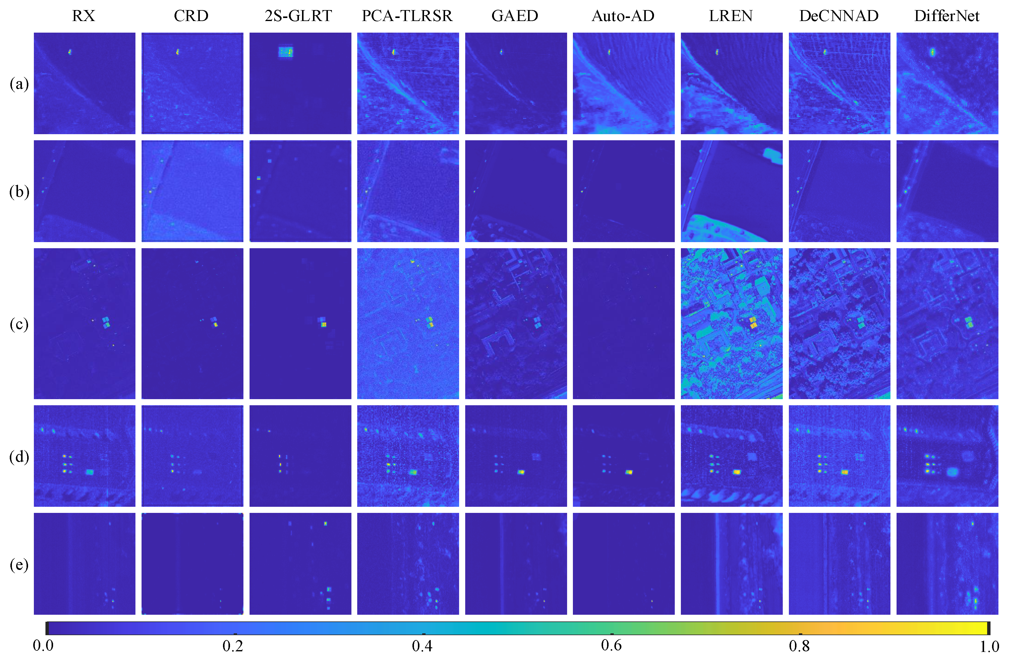
In this section, the detection performance of the proposed method is analyzed compared with eight state-of-the-art methods, including the RX, the CRD, the 2S-GLRT, the PCA-TLRSR, the GAED, the Auto-AD, the LREN, and the DeCNNAD. The detection results of these methods are shown in Figure 8.
As shown in Figure 8, in the results of the RX method, the background is relatively clean, but the anomaly targets are not completely detected. This is due to the common occurrence of spectral mixing in real datasets, resulting in spectral interference from background pixels around the targets. Such interference can impact the overall detection performance. Similar detection performance also exists in the results of CRD, GAED, and Auto-AD. In the results of 2S-GLRT, the contour information of the anomalies is lost. This is attributed to the fact that the features in the local inner window change slowly as the window slides across the HSI, causing block effects. In the results of the PCA-TLRSR method, there are some noises in the detection results. This is because that the low-rank and sparse decomposition theory is adopted in the PCA-TLRSR. The sparse matrix contains both anomalies and noises. As a result, it is hard for the PCA-TLRSR to distinguish the targets and noises. In the results of the LREN method, the background is clear. This is because this method constructs a global lowest rank dictionary. When the background is complex, the constructed dictionary is not comprehensive enough for the background, resulting in the inability to fully represent background components. This leads to insufficient background suppression. In the results of the DeCNNAD method, the background is clear and there are some noises in the results. This is because a denoiser is adopted in this method to obtain the background dictionary. The quality of the constructed dictionary depends on the performance of the denoiser. When the denoiser removes certain edges in the scene, the reconstructed background also loses these edges, leaving some background edges in the detection results. Furthermore, noises and anomalies are not distinguished in this method. This leads to some noises existing in the detection results.
Specifically, for the Bay Champagne dataset, the anomaly targets in the detection results of RX, GAED, Auto-AD, and LREN are not fully detected. The contours of the anomaly targets in the detection result of 2S-GLRT are lost. The background in the result of PCA-TLRSR is clear. The detection results of CRD and proposed DifferNet are satisfactory. For the Pavia dataset, the anomaly targets are not well separated from the background in the results of RX, CRD, GAED, Auto-AD, and DeCNNAD. The shape of the targets is lost in the result of 2S-GLRT. The distinctiveness between the anomalies and background is not significant in the result of PCA-TLRSR. The background in the result of LREN is clear. In the result of the proposed DifferNet, all the anomaly targets are highlighted compared with the background. For the dataset of MUUFLGulfport, the Auto-AD method fails to detect the anomaly targets. The background is suppressed in the results of the CRD and 2S-GLRT methods, but the anomaly targets are partially suppressed as well. In the results of the RX and PCA-TLRSR methods, the roof at the top of the scene is enhanced incorrectly. In the results of the GAED and DeCNNAD methods, the anomaly targets are not well distinguished from the background. The background is clear in the result of LREN. In the result of the proposed DifferNet method, the anomaly targets are well separated from the background. For the dataset of SpecTIR, the small targets are submerged in the background in the results of RX, CRD, 2S-GLRT, PCA-TLRSR, LREN, and DeCNNAD. There are some noises in the results of PCA-TLRSR and DeCNNAD. In the results of PCA-TLRSR, GAED, Auto-AD, LREN, and DeCNNAD, a square background in the middle of the scene is not suppressed. In the result of the proposed method, the detection performance is satisfactory. For the dataset of WHU-Hi-River, the anomaly targets are not well detected in the results of CRD, GAED, and Auto-AD. In the results of RX, LREN, and DeCNNAD, the distinction between the targets and background is not significant. The background is clear in the results of PCA-TLRSR, LREN, and DeCNNAD. The shape of the anomaly targets is changed in the result of 2S-GLRT. The proposed DifferNet obtains a satisfactory detection result. Overall, the proposed method obtains superior results on the five datasets compared with other state-of-the-art methods.
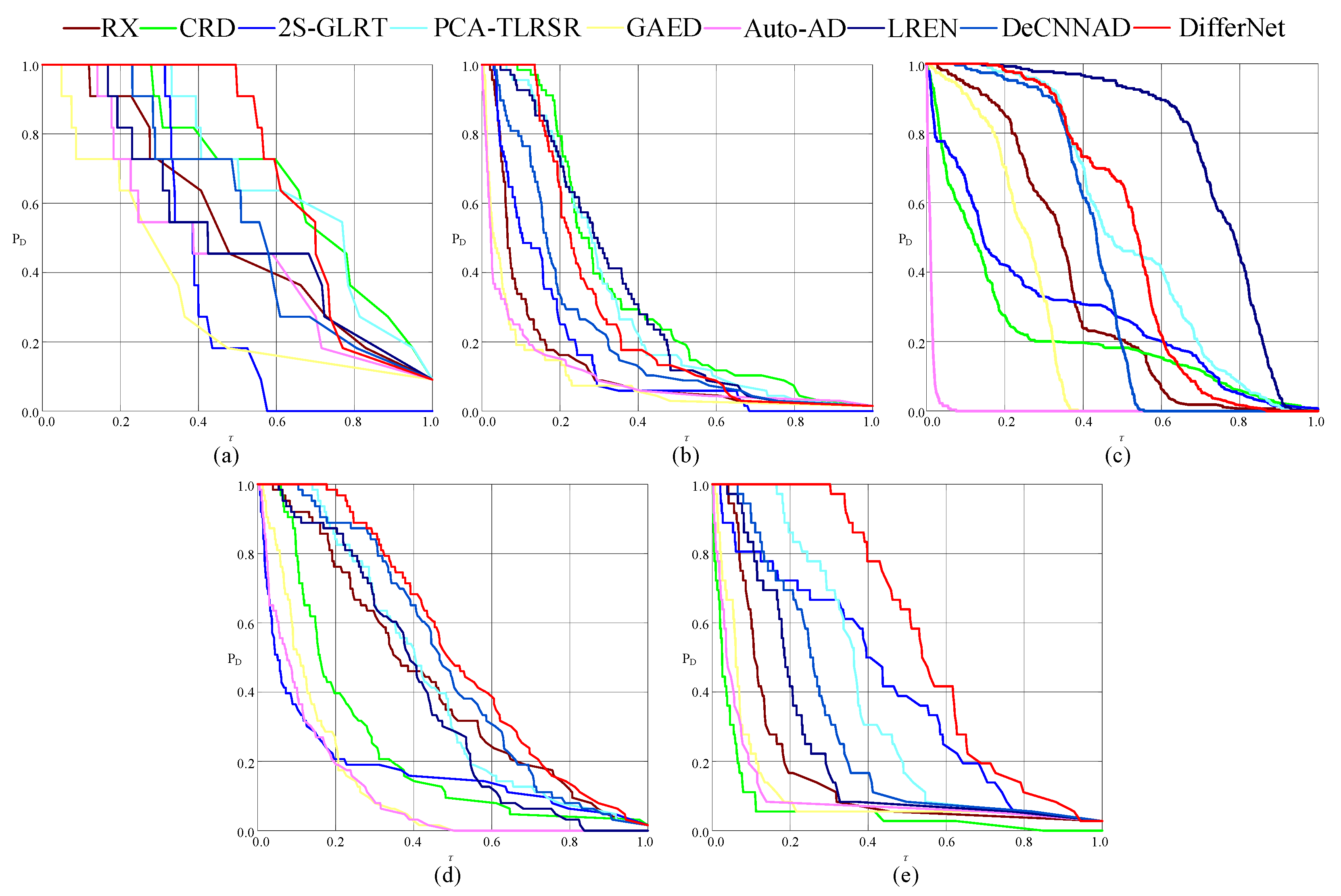
From the objective evaluation perspective, 3D ROC curves and AUC values are adopted to evaluate the performance of the methods. The 3D ROC curves ( P D , P F , τ ) on different datasets are shown in Figure 9. The curves of the proposed method marked in red are higher than those of the other methods on the datasets of Bay Champagne and WHU-Hi-River. On the other datasets, the curves of the proposed DifferNet are close to those of the other methods.
The 2D ROC curves ( P D , P F ) on different datasets are shown in Figure 10. The corresponding A U C ( D , F ) values are shown in Table 1. As shown in Figure 10, the ( P D , P F ) curves of the proposed DifferNet marked in red are higher than those of the other methods on the datasets of Bay Champagne, Pavia, SpecTIR, and WHU-Hi-River. On the dataset of MUUFLGulfport, the curves of the proposed method and comparison methods are mixed, but the curve of the proposed method is at the upper part of all the curves. In Table 1, the best A U C ( D , F ) values are in bold. The proposed method achieves the best A U C ( D , F ) on all the datasets. This means that the proposed method achieves a high detection rate at a low false alarm rate. Compared with the second-best values, the A U C ( D , F ) values of the proposed method are higher by 0.0001, 0.0105, 0.0006, 0.0110, and 0.0005 on the five datasets, respectively. Overall, the performance of the proposed method is excellent.
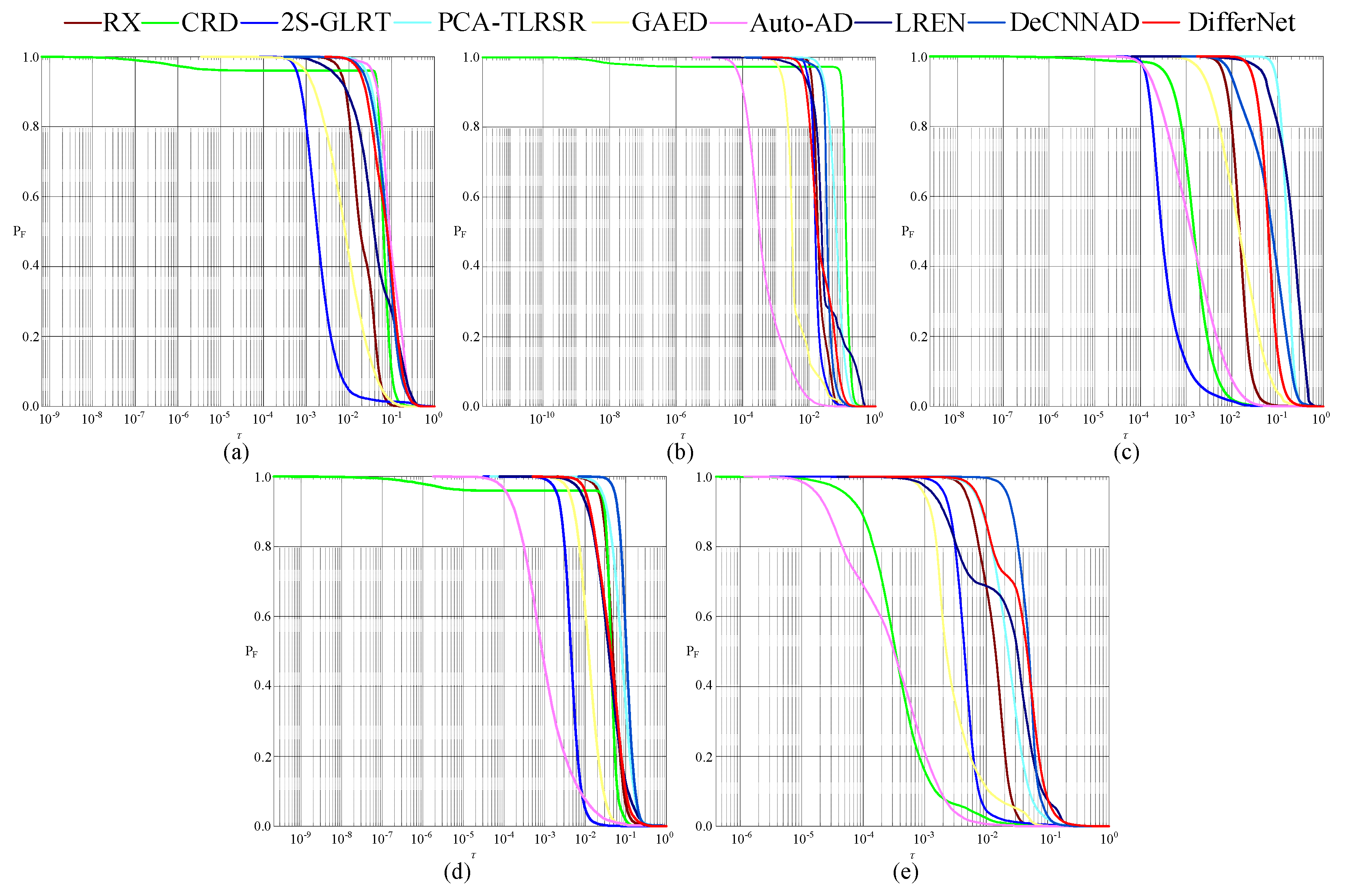
The 2D ROC curves ( P D , τ ) on different datasets are shown in Figure 11. The corresponding A U C ( D , τ ) values are shown in Table 2. As shown in Figure 11, the ( P D , τ ) curves of the proposed DifferNet marked in red are higher than those of the other methods on the datasets of Bay Champagne, SpecTIR, and WHU-Hi-River. On the datasets of Pavia and MUUFLGulfport, the curves of the proposed method are not at the top of all the curves. However, the curves of the proposed method are at the upper part of all the curves. In Table 2, the best A U C ( D , τ ) values are in bold. The proposed method achieves the best A U C ( D , τ ) values on the datasets of Bay Champagne, SpecTIR, and WHU-Hi-River, which are higher by 0.0108, 0.0425, and 0.1588 compared with the second-best values, respectively. On the datasets of Pavia and MUUFLGulfport, the CRD method and the LREN method achieve the best values, respectively. The best values on the two datasets are higher by 0.0603 and 0.2393 than that of the proposed method, respectively. As a result, the proposed DifferNet has a good detection rate compared with the other methods.
The 2D ROC curves ( P F , τ ) on different datasets are shown in Figure 12. The corresponding A U C ( F , τ ) values are shown in Table 3. As shown in Figure 12, the ( P F , τ ) curves of the proposed DifferNet marked in red are mixed with those of the comparison methods on the five datasets, which are neither the highest nor the lowest. On the datasets of Bay Champagne and MUUFLGulfport, the curve of the 2S-GLRT is the lowest one among all the curves. On the datasets of Pavia and SpecTIR, the curve of the Auto-AD is lower than the other 2D ROC curves. On the dataset of WHU-Hi-River, the curves of CRD and Auto-AD are relatively lower than those of the other methods. In Table 3, the best A U C ( F , τ ) values are in bold. On the datasets of Bay Champagne, MUUFLGulfport, and SpecTIR, the 2S-GLRT achieves the minimum A U C ( F , τ ) values of 0.0080, 0.0011, and 0.0052, which are lower by 0.0839, 0.0706, and 0.0477 than those of the proposed method. On the datasets of Pavia and WHU-Hi-River, the Auto-AD method achieves the minimum A U C ( F , τ ) values of 0.0013 and 0.0008, which are lower by 0.0326 and 0.0496 than those of the proposed method. The A U C ( F , τ ) values of the proposed method on the five datasets are between the maximum value and the minimum value, respectively. This means that the proposed method has a certain background suppression capability. Overall, the proposed DifferNet method obtains satisfactory and advanced detection results.
To evaluate the execution efficiency of all the methods, the time consumption of all the methods on the five datasets is evaluated. It is worth noting that Auto-AD, LREN, and the proposed method are implemented by Python 3. The rest of the methods are conducted using Matlab 2022b. All the methods are executed on a computer with an Intel CoreTM i9-12900H produced by Intel the United States, 16 GB RAM produced by Samsung South Korea, and NVDIA GeForce RTX 3060 Laptop GPU produced by Lenovo China. We measure the speed of the methods both with and without GPU acceleration separately. The time consumption results are shown in Table 4, and the best values are in bold. The results show that the RX method has the fastest processing speed without GPU acceleration. With the acceleration of GPU, the DeCNNAD method achieves the best time performance on the dataset of MUUFLGulfport, and the Auto-AD method achieves the best time performance on the rest of the datasets. The time consumption is relatively high compared with other methods without GPU acceleration, and it has an acceptable running speed with GPU acceleration. In the future, we need to further optimize the DifferNet to improve efficiency and detection performance.
The initialization of weights and bias in the CNN directly affects the detection performance. To investigate the stability of the proposed method under different initialization conditions, we remove the fixed random seed and conduct 20 repeated experiments. We record the range of A U C ( D , F ) values obtained, and the statistical results are shown in Table 5.
As shown in Table 5, the proposed method exhibits relatively low variance and range across 20 experiments. This means that the proposed method has good parameter stability.
To demonstrate the noise robustness of the proposed method, we conduct experiments by adding various types of noise to the original dataset. The added noises are the Gaussian noise with mean 0 and variance 0.01, salt and pepper noise with density 0.01, and uniform multiplicative noise with mean 0 and variance 0.01. The detection results are shown in Figure 13 and Table 6. To further illustrate the false alarm rates of these methods, we also calculate the false positive rate (FPR), while the detection rate is 0.9. The results are shown in Table 7.
As shown in Figure 13, the results of input without noises are the best detection results. When the Gaussian noises are added to the input datasets, the detection performance decreases. When the salt and pepper noises are added to the inputs, the detection results are slightly better than those of inputs with Gaussian noises. When the multiplicative noises are added to the inputs, the detection results are better than those of inputs with salt and pepper noises. Despite the interference of noises with the detection results, the anomaly targets can still be detected. In Table 6, on the datasets of Bay Champagne, Pavia, and WHU-Hi-River, the performance of inputs with salt and pepper noises is better than inputs with the rest of the noises. On the datasets of MUUFLGulfport and SpecTIR, the performance of inputs with multiplicative noises is better than inputs with rest of the noises. The Gaussian noises have the greatest impact on the detection performance. In Table 7, the FPR values of inputs without noise are low. With Gaussian noises, the FPR values increase significantly compared with other noises. The impact of salt and pepper noises and multiplicative noises on the FPR values is similar. As a result, Gaussian noise has a significant impact on the performance of the proposed method, while salt and pepper noise and multiplicative noise have relatively minor effects on the proposed method. The noise robustness of the proposed method is acceptable.

3.5. Ablation Analysis

In this section, the attention module effectiveness and the structure effectiveness are discussed.
To investigate the effectiveness of the attention module, the DifferNet without any attention and DifferNet with only one type of attention in different positions are compared with the proposed DifferNet. The A U C ( D , F ) is adopted to evaluate the detection performance. The detection results of these methods are shown in Figure 14. In Figure 14, L T A i , i = 1 , 2 , 3 denotes that the local Transformer attention (LTA) is added after the i-th convolutional layer, and L D A i , i = 1 , 2 , 3 denotes that the local detail attention (LDA) is added after the i-th convolutional layer. Although the results of these methods are close to each other, background edges still remain in the results of DifferNet without attention and DifferNet with LTA. This means that the LDA module can preserve the background edges well so that the residual map contains few background edges. In addition, the anomaly targets are not complete and prominent in the results of DifferNet with LDA. This demonstrates that the LTA is capable of effectively focusing on the primary information within the local window. It can enhance the expressive ability of CNN, making our DifferNet model the background accurately. The corresponding A U C ( D , F ) values are shown in Table 8. The DifferNet with both LTA and LDA achieves the best values on the five datasets. The experimental results show that the LTA can improve the expressive ability of CNN and facilitate precise modeling of the background. The LDA can enhance the ability of the network to represent background edges. Both attention modules are effective in anomaly detection.
To further demonstrate the efficiency of the proposed LTA module, we assess the time consumption and storage occupancy in comparison to the traditional Transformer model. The evaluation is conducted on inputs with spatial sizes of 100 × 100 and 150 × 150 . The results are shown in Table 9. The results show that the proposed LTA exhibits significant advantages over traditional Transformer in terms of both time consumption and spatial occupancy.
To investigate the effectiveness of the differential structure of the DifferNet, the network only with 3 × 3 convolution kernels and the network only with 5 × 5 convolution kernels are compared with the DifferNet without attention. The loss functions of these methods include a smooth L1 function. The A U C ( D , F ) is adopted as the evaluation indicator. The detection results are shown in Figure 15. The anomaly targets in the results of 3 × 3 convolution and 5 × 5 convolution are not prominent compared with the differential convolution. This means that the differential convolution is effective in preserving anomaly information. The A U C ( D , F ) values are shown in Table 10. The differential convolution achieves the best detection performance compared with standard 3 × 3 and 5 × 5 convolution. As such, the framework of the proposed method is effective and excellent in the anomaly detection field.
To further illustrate the effectiveness of differential convolution for anomaly detection, we apply the differential convolution (DC) to the Auto-AD method. Specifically, all the 3 × 3 convolutions are replaced by 3 × 3 and 5 × 5 convolutions, and the difference operation is adopted in the decoder part of the Auto-AD. The experimental results are shown in Figure 16. The corresponding A U C ( D , F ) values are shown in Table 11.
As shown in Figure 16, the background in the results of Auto-AD with DC is suppressed. The anomaly targets are highlighted on the five datasets. The performance of the Auto-AD with DC is better than that of Auto-AD. The AUC values in Table 11 show that the differential convolution can improve the performance of Auto-AD on most of the datasets. These experiments demonstrate that the differential convolution is effective.

4. Conclusions

In this work, a hyperspectral anomaly detection method based on differential network is proposed. Firstly, 5 × 5 and 3 × 3 convolutional kernels are employed separately to extract outer window features and inner window features. Secondly, to enhance the expression capability of internal window features for details and important information, outer window features are utilized to guide inner window features, and two local guidance attention modules are introduced. Specifically, the local detail attention module enhances the extraction capability of inner window features for edge details, while the local Transformer attention module boosts the focusing ability of inner window features on salient information. Thirdly, weighted difference is applied to the obtained outer and inner window features to derive differential features. These differential features represent local punctured neighborhood characteristics in the HSI, facilitating the reconstruction of a clean background. Fourthly, by concatenating all differential features along the channel dimension and applying a 1 × 1 convolution for feature fusion, the background HSI is obtained. Finally, anomaly detection results are obtained from the residuals between the input HSI and the background HSI. Comparative experiments with eight state-of-the-art methods are conducted on five real-world datasets. The experimental results demonstrate that the proposed method enhances anomalies while suppressing background. The proposed method achieves superior performance in terms of the detection results, including ROC curves and AUC values. Ablation studies indicate that each part of the proposed method contributes positively to detection performance. The proposed method provides a novel differential structure and decomposes the background reconstruction task into two steps for the first time, including comprehensive feature representation and background feature extraction. It can avoid the problem that anomaly features interfere with the background reconstruction. Furthermore, the two proposed guidance attention modules can ensure the completeness of feature extraction. These methods can provide researchers with inspiring ideas and drive the development in the field of hyperspectral anomaly detection. However, the proposed method performs poorly in terms of execution efficiency, affecting its practical applicability in engineering. In our future work, we plan to conduct further research on network architecture, streamline the structure, and enhance the efficiency of the method while maintaining detection effectiveness.

Author Contributions

Conceptualization, J.Z., P.X. and X.T.; methodology, J.Z.; software, J.Z.; validation, X.T., J.Z. and W.T.; formal analysis, J.Z., P.X. and X.T.; investigation, J.Z.; resources, X.T.; data curation, J.Z. and P.X.; writing—original draft preparation, J.Z.; writing—review and editing, P.X., D.Z. and H.L.; visualization, J.Z. and P.X.; supervision, H.Z.; project administration, H.L., J.S. and H.Z.; funding acquisition, D.Z., H.L., J.S. and H.Z. All authors have read and agreed to the published version of the manuscript.

Funding

This research was funded by the 111 Project (B17035), Aeronautical Science Foundation of China (201901081002), Youth Foundation of Shaanxi Province (2021JQ-182), the Natural Science Foundation of Jiangsu Province (BK20210064), the Wuxi Innovation and Entrepreneurship Fund “Taihu Light” Science and Technology (Fundamental Research) Project (K20221046), the Start-up Fund for Introducing Talent of Wuxi University (2021r007), National Natural Science Foundation of China (62001443, 62105258), Natural Science Foundation of Shandong Province (ZR2020QE294), the Fundamental Research Funds for the Central Universities (QTZX23059, QTZX23009), the Basic Research Plan of Natural Science in Shaanxi Province (2023-JC-YB-062), Research Scholarship Fund of Xidian University.

Data Availability Statement

Data are available from the corresponding author upon reasonable request or from the data publishers as shown in the paper.

Conflicts of Interest

The authors declare no conflicts of interest.

References

  1. Xiang, P.; Zhou, H.; Li, H.; Song, S.; Tan, W.; Song, J.; Gu, L. Hyperspectral anomaly detection by local joint subspace process and support vector machine. Int. J. Remote Sens. 2020, 41, 3798–3819. [Google Scholar] [CrossRef]
  2. Xiao, Q.; Zhao, L.; Chen, S.; Li, X. Robust Tensor Low-Rank Sparse Representation with Saliency Prior for Hyperspectral Anomaly Detection. IEEE Trans. Geosci. Remote Sens. 2023. [Google Scholar] [CrossRef]
  3. Guan, J.; Lai, R.; Li, H.; Yang, Y.; Gu, L. DnRCNN: Deep recurrent convolutional neural network for HSI destriping. IEEE Trans. Neural Netw. Learn. Syst. 2022, 34, 3255–3268. [Google Scholar] [CrossRef]
  4. Xiang, P.; Song, J.; Li, H.; Gu, L.; Zhou, H. Hyperspectral anomaly detection with harmonic analysis and low-rank decomposition. Remote Sens. 2019, 11, 3028. [Google Scholar] [CrossRef]
  5. Zhang, Z.; Hu, B.; Wang, M.; Arun, P.V.; Zhao, D.; Zhu, X.; Hu, J.; Li, H.; Zhou, H.; Qian, K. Hyperspectral Video Tracker Based on Spectral Deviation Reduction and a Double Siamese Network. Remote Sens. 2023, 15, 1579. [Google Scholar] [CrossRef]
  6. Zhao, D.; Zhu, X.; Zhang, Z.; Arun, P.V.; Cao, J.; Wang, Q.; Zhou, H.; Jiang, H.; Hu, J.; Qian, K. Hyperspectral video target tracking based on pixel-wise spectral matching reduction and deep spectral cascading texture features. Signal Process. 2023, 209, 109033. [Google Scholar] [CrossRef]
  7. Zhang, Z.; Zhu, X.; Zhao, D.; Arun, P.V.; Zhou, H.; Qian, K.; Hu, J. Hyperspectral Video Target Tracking Based on Deep Features with Spectral Matching Reduction and Adaptive Scale 3D Hog Features. Remote Sens. 2022, 14, 5958. [Google Scholar] [CrossRef]
  8. Lin, S.; Zhang, M.; Cheng, X.; Shi, L.; Gamba, P.; Wang, H. Dynamic Low-Rank and Sparse Priors Constrained Deep Autoencoders for Hyperspectral Anomaly Detection. IEEE Trans. Instrum. Meas. 2023, 73, 2500518. [Google Scholar] [CrossRef]
  9. Zhao, D.; Cao, J.; Zhu, X.; Zhang, Z.; Arun, P.V.; Guo, Y.; Qian, K.; Zhang, L.; Zhou, H.; Hu, J. Hyperspectral Video Target Tracking Based on Deep Edge Convolution Feature and Improved Context Filter. Remote Sens. 2022, 14, 6219. [Google Scholar] [CrossRef]
  10. Xu, K.; Zhang, H.; Li, Y.; Zhang, Y.; Lai, R.; Liu, Y. An ultra-low power tinyml system for real-time visual processing at edge. IEEE Trans. Circ. Syst. II-Express Briefs 2023, 70, 2640–2644. [Google Scholar] [CrossRef]
  11. Wang, L.; Wang, Y.; Li, Z.; Wu, C.; Xu, M.; Shao, M. Eliminating spatial correlations of anomaly: Corner-Visible Network for Unsupervised Hyperspectral Anomaly Detection. IEEE Trans. Geosci. Remote Sens. 2023, 61, 5529114. [Google Scholar] [CrossRef]
  12. Zhu, X.; Zhang, H.; Hu, B.; Huang, K.; Arun, P.V.; Jia, X.; Zhao, D.; Wang, Q.; Zhou, H.; Yang, S. DSP-Net: A dynamic spectral-spatial joint perception network for hyperspectral target tracking. IEEE Geosci. Remote Sens. Lett. 2023, 20, 5510905. [Google Scholar] [CrossRef]
  13. Xiang, P.; Li, H.; Song, J.; Wang, D.; Zhang, J.; Zhou, H. Spectral–Spatial complementary decision fusion for hyperspectral anomaly detection. Remote Sens. 2022, 14, 943. [Google Scholar] [CrossRef]
  14. Wu, Z.; Wang, B. Background Reconstruction via 3D-Transformer Network for Hyperspectral Anomaly Detection. Remote Sens. 2023, 15, 4592. [Google Scholar] [CrossRef]
  15. Wang, N.; Shi, Y.; Li, H.; Zhang, G.; Li, S.; Liu, X. Multi-Prior Graph Autoencoder with Ranking-Based Band Selection for Hyperspectral Anomaly Detection. Remote Sens. 2023, 15, 4430. [Google Scholar] [CrossRef]
  16. Li, Y.; Jiang, K.; Xie, W.; Lei, J.; Zhang, X.; Du, Q. A Model-Driven Deep Mixture Network for Robust Hyperspectral Anomaly Detection. IEEE Trans. Geosci. Remote Sens. 2023, 61, 5522916. [Google Scholar] [CrossRef]
  17. Wang, X.; Wang, Y.; Mu, Z.; Wang, M. FCAE-AD: Full Convolutional Autoencoder Based on Attention Gate for Hyperspectral Anomaly Detection. Remote Sens. 2023, 15, 4263. [Google Scholar] [CrossRef]
  18. Yang, X.; Tu, B.; Li, Q.; Li, J.; Plaza, A. Graph Evolution-Based Vertex Extraction for Hyperspectral Anomaly Detection. IIEEE Trans. Neural Netw. Learn. Syst. 2023, 1–15. [Google Scholar] [CrossRef]
  19. Su, H.; Wu, Z.; Zhang, H.; Du, Q. Hyperspectral anomaly detection: A survey. IEEE Geosci. Remote Sens. Mag. 2021, 10, 64–90. [Google Scholar] [CrossRef]
  20. Tu, B.; Yang, X.; Zhou, C.; He, D.; Plaza, A. Hyperspectral anomaly detection using dual window density. IEEE Trans. Geosci. Remote Sens. 2020, 58, 8503–8517. [Google Scholar] [CrossRef]
  21. Chang, C.I. Hyperspectral anomaly detection: A dual theory of hyperspectral target detection. IEEE Trans. Geosci. Remote Sens. 2021, 60, 5511720. [Google Scholar] [CrossRef]
  22. Li, S.; Zhang, K.; Duan, P.; Kang, X. Hyperspectral anomaly detection with kernel isolation forest. IEEE Trans. Geosci. Remote Sens. 2019, 58, 319–329. [Google Scholar] [CrossRef]
  23. Matteoli, S.; Diani, M.; Corsini, G. A tutorial overview of anomaly detection in hyperspectral images. IEEE Aerosp. Electron. Syst. Mag. 2010, 25, 5–28. [Google Scholar] [CrossRef]
  24. Salem, M.B.; Ettabaa, K.S.; Hamdi, M.A. Anomaly detection in hyperspectral imagery: An overview. In Proceedings of the International Image Processing, Applications and Systems Conference, Sfax, Tunisia, 5–7 November 2014; pp. 1–6. [Google Scholar]
  25. Reed, I.S.; Yu, X. Adaptive multiple-band CFAR detection of an optical pattern with unknown spectral distribution. IEEE Trans. Acoust. Speech Signal Process. 1990, 38, 1760–1770. [Google Scholar] [CrossRef]
  26. Molero, J.M.; Garzon, E.M.; Garcia, I.; Plaza, A. Analysis and optimizations of global and local versions of the RX algorithm for anomaly detection in hyperspectral data. IEEE J. Sel. Top. Appl. Earth Observ. Remote Sens. 2013, 6, 801–814. [Google Scholar] [CrossRef]
  27. Kwon, H.; Nasrabadi, N.M. Kernel RX-algorithm: A nonlinear anomaly detector for hyperspectral imagery. IEEE Trans. Geosci. Remote Sens. 2005, 43, 388–397. [Google Scholar] [CrossRef]
  28. Kwon, H.; Nasrabadi, N.M. Hyperspectral anomaly detection using kernel RX-algorithm. In Proceedings of the 2004 International Conference on Image Processing, 2004, ICIP ’04, Singapore, 24–27 October 2004; Volume 5, pp. 3331–3334. [Google Scholar]
  29. Liu, J.; Hou, Z.; Li, W.; Tao, R.; Orlando, D.; Li, H. Multipixel anomaly detection with unknown patterns for hyperspectral imagery. IEEE Trans. Neural Netw. Learn. Syst. 2021, 33, 5557–5567. [Google Scholar] [CrossRef]
  30. Wang, S.; Hu, X.; Sun, J.; Liu, J. Hyperspectral anomaly detection using ensemble and robust collaborative representation. Inf. Sci. 2023, 624, 748–760. [Google Scholar] [CrossRef]
  31. Li, W.; Du, Q. Collaborative representation for hyperspectral anomaly detection. IEEE Trans. Geosci. Remote Sens. 2014, 53, 1463–1474. [Google Scholar] [CrossRef]
  32. Peng, J.; Sun, W.; Li, H.C.; Li, W.; Meng, X.; Ge, C.; Du, Q. Low-rank and sparse representation for hyperspectral image processing: A review. IEEE Geosci. Remote Sens. Mag. 2021, 10, 10–43. [Google Scholar] [CrossRef]
  33. Su, H.; Wu, Z.; Zhu, A.X.; Du, Q. Low rank and collaborative representation for hyperspectral anomaly detection via robust dictionary construction. ISPRS-J. Photogramm. Remote Sens. 2020, 169, 195–211. [Google Scholar] [CrossRef]
  34. Zhang, Y.; Du, B.; Zhang, L.; Wang, S. A low-rank and sparse matrix decomposition-based Mahalanobis distance method for hyperspectral anomaly detection. IEEE Trans. Geosci. Remote Sens. 2015, 54, 1376–1389. [Google Scholar] [CrossRef]
  35. Wang, M.; Wang, Q.; Hong, D.; Roy, S.K.; Chanussot, J. Learning tensor low-rank representation for hyperspectral anomaly detection. IEEE Trans. Cybern. 2022, 53, 679–691. [Google Scholar] [CrossRef] [PubMed]
  36. Zhang, L.; Ma, J.; Cheng, B.; Lin, F. Fractional fourier transform-based tensor RX for hyperspectral anomaly detection. Remote Sens. 2022, 14, 797. [Google Scholar] [CrossRef]
  37. Xu, Y.; Zhang, L.; Du, B.; Zhang, L. Hyperspectral anomaly detection based on machine learning: An overview. IEEE J. Sel. Top. Appl. Earth Observ. Remote Sens. 2022, 15, 3351–3364. [Google Scholar] [CrossRef]
  38. Hu, X.; Xie, C.; Fan, Z.; Duan, Q.; Zhang, D.; Jiang, L.; Wei, X.; Hong, D.; Li, G.; Zeng, X.; et al. Hyperspectral anomaly detection using deep learning: A review. Remote Sens. 2022, 14, 1973. [Google Scholar] [CrossRef]
  39. Xie, W.; Zhang, X.; Li, Y.; Lei, J.; Li, J.; Du, Q. Weakly supervised low-rank representation for hyperspectral anomaly detection. IEEE Trans. Cybern. 2021, 51, 3889–3900. [Google Scholar] [CrossRef]
  40. Li, W.; Wu, G.; Du, Q. Transferred deep learning for anomaly detection in hyperspectral imagery. IEEE Geosci. Remote Sens. Lett. 2017, 14, 597–601. [Google Scholar] [CrossRef]
  41. Rao, W.; Gao, L.; Qu, Y.; Sun, X.; Zhang, B.; Chanussot, J. Siamese transformer network for hyperspectral image target detection. IEEE Trans. Geosci. Remote Sens. 2022, 60, 5526419. [Google Scholar] [CrossRef]
  42. Xiang, P.; Ali, S.; Jung, S.K.; Zhou, H. Hyperspectral anomaly detection with guided autoencoder. IEEE Trans. Geosci. Remote Sens. 2022, 60, 5538818. [Google Scholar] [CrossRef]
  43. Wang, S.; Wang, X.; Zhang, L.; Zhong, Y. Auto-AD: Autonomous hyperspectral anomaly detection network based on fully convolutional autoencoder. IEEE Trans. Geosci. Remote Sens. 2021, 60, 5503314. [Google Scholar] [CrossRef]
  44. Jiang, K.; Xie, W.; Lei, J.; Jiang, T.; Li, Y. LREN: Low-rank embedded network for sample-free hyperspectral anomaly detection. AAAI Conf. Artif. Intell. 2021, 35, 4139–4146. [Google Scholar] [CrossRef]
  45. Fu, X.; Jia, S.; Zhuang, L.; Xu, M.; Zhou, J.; Li, Q. Hyperspectral anomaly detection via deep plug-and-play denoising CNN regularization. IEEE Trans. Geosci. Remote Sens. 2021, 59, 9553–9568. [Google Scholar] [CrossRef]
  46. Zhang, Y.; Li, D.; Shi, X.; He, D.; Song, K.; Wang, X.; Qin, H.; Li, H. Kbnet: Kernel basis network for image restoration. arXiv 2023, arXiv:2303.02881. [Google Scholar]
  47. Chen, L.; Chu, X.; Zhang, X.; Sun, J. Simple baselines for image restoration. In European Conference on Computer Vision; Springer: Cham, Switzerland, 2022; pp. 17–33. [Google Scholar]
  48. Dosovitskiy, A.; Beyer, L.; Kolesnikov, A.; Weissenborn, D.; Zhai, X.; Unterthiner, T.; Dehghani, M.; Minderer, M.; Heigold, G.; Gelly, S.; et al. An image is worth 16 × 16 words: Transformers for image recognition at scale. arXiv 2020, arXiv:2010.11929. [Google Scholar]
  49. Vaswani, A.; Shazeer, N.; Parmar, N.; Uszkoreit, J.; Jones, L.; Gomez, A.N.; Kaiser, Ł.; Polosukhin, I. Attention is all you need. Adv. Neural Inf. Process. Syst. 2017, 30, 5999–6009. [Google Scholar]
  50. Mao, X.; Qi, G.; Chen, Y.; Li, X.; Duan, R.; Ye, S.; He, Y.; Xue, H. Towards robust vision transformer. In Proceedings of the IEEE/CVF Conference on Computer Vision and Pattern Recognition (CVPR), New Orleans, LA, USA, 18–24 June 2022; pp. 12042–12051. [Google Scholar]
  51. Schmidt, M.; Fung, G.; Rosales, R. Fast optimization methods for l1 regularization: A comparative study and two new approaches. In Proceedings of the Machine Learning: ECML 2007: 18th European Conference on Machine Learning, Warsaw, Poland, 17–21 September 2007; Proceedings 18. Springer: Berlin/Heidelberg, Germany, 2007; pp. 286–297. [Google Scholar]
  52. Kang, X.; Zhang, X.; Li, S.; Li, K.; Li, J.; Benediktsson, J.A. Hyperspectral anomaly detection with attribute and edge-preserving filters. IEEE Trans. Geosci. Remote Sens. 2017, 55, 5600–5611. [Google Scholar] [CrossRef]
  53. Herwegab, J.A.; Kerekesa, J.P.; Weatherbeec, O.; Messingera, D.; van Aardta, J.; Ientiluccia, E.; Ninkova, Z.; Faulringa, J.; Raquenoa, N.; Meolad, J. Spectir hyperspectral airborne rochester experiment data collection campaign. In Proceedings of the SPIE, Bellingham, WA, USA, 27 December 2012. [Google Scholar]
  54. Wang, S.; Wang, X.; Zhong, Y.; Zhang, L. Hyperspectral anomaly detection via locally enhanced low-rank prior. IEEE Trans. Geosci. Remote Sens. 2020, 58, 6995–7009. [Google Scholar] [CrossRef]
  55. Gader, P.; Zare, A.; Close, R.; Aitken, J.; Tuell, G. Muufl Gulfport Hyperspectral and Lidar Airborne Data Set; Tech. Rep. REP-2013-570; University Florida: Gainesville, FL, USA, 2013. [Google Scholar]
  56. Du, X.; Zare, A. Technical Report: Scene Label Ground Truth Map for MUUFL Gulfport Data Set; University of Florida: Gainesville, FL, USA, 2017. [Google Scholar]
  57. Chang, C.I. An effective evaluation tool for hyperspectral target detection: 3D receiver operating characteristic curve analysis. IEEE Trans. Geosci. Remote Sens. 2020, 59, 5131–5153. [Google Scholar] [CrossRef]
Figure 1. The whole structure of the proposed DifferNet.
Remotesensing 16 00434 g001
Figure 2. The proposed local detail attention.
Remotesensing 16 00434 g002
Figure 3. The proposed local Transformer attention.
Remotesensing 16 00434 g003
Figure 4. Pseudo-color image and the ground truth of four datasets: (a) Bay Champagne; (b) Pavia; (c) SpecTIR; (d) WHU-Hi-River.
Remotesensing 16 00434 g004
Figure 5. Pseudo-color image and the ground truth of the MUUFLGulfport dataset: (a) pseudo-color image; (b) ground truth.
Remotesensing 16 00434 g005
Figure 6. Effects of the number of base convolutional kernels n b a s e and the number of group channels c g r o u p on the performance of the proposed method for different datasets: (a) Bay Champagne; (b) Pavia; (c) MUUFLGulfport; (d) SpecTIR; (e) WHU-Hi-River.
Remotesensing 16 00434 g006
Figure 7. Effects of the local detail attention position p l d and the local Transformer position p l t on the performance of the proposed method for different datasets: (a) Bay Champagne; (b) Pavia; (c) MUUFLGulfport; (d) SpecTIR; (e) WHU-Hi-River.
Remotesensing 16 00434 g007
Figure 8. Detection performance of different methods on five datasets: (a) Bay Champagne; (b) Pavia; (c) MUUFLGulfport; (d) SpecTIR; (e) WHU-Hi-River.
Remotesensing 16 00434 g008
Figure 9. 3D ROC curves ( P D , P F , τ ) on the five datasets: (a) Bay Champagne; (b) Pavia; (c) MUUFLGulfport; (d) SpecTIR; (e) WHU-Hi-River.
Remotesensing 16 00434 g009
Figure 10. 2D ROC curves ( P D , P F ) on the five datasets: (a) Bay Champagne; (b) Pavia; (c) MUUFLGulfport; (d) SpecTIR; (e) WHU-Hi-River.
Remotesensing 16 00434 g010
Figure 11. 2D ROC curves ( P D , τ ) on the five datasets: (a) Bay Champagne; (b) Pavia; (c) MUUFLGulfport; (d) SpecTIR; (e) WHU-Hi-River.
Remotesensing 16 00434 g011
Figure 12. 2D ROC curves ( P F , τ ) on the five datasets: (a) Bay Champagne; (b) Pavia; (c) MUUFLGulfport; (d) SpecTIR; (e) WHU-Hi-River.
Remotesensing 16 00434 g012
Figure 13. Detection performance on five datasets with different noises: (a) without noise; (b) with Gaussian noise; (c) with salt and pepper noise; (d) with uniform multiplicative noise.
Remotesensing 16 00434 g013
Figure 14. Detection results of the proposed method with different attentions on the five datasets: (a) Bay Champagne; (b) Pavia; (c) MUUFLGulfport; (d) SpecTIR; (e) WHU-Hi-River.
Remotesensing 16 00434 g014
Figure 15. Detection results of the differential convolution and standard convolution on the five datasets: (a) 5 × 5 convolution; (b) 3 × 3 convolution; (c) differential convolution.
Remotesensing 16 00434 g015
Figure 16. Detection results of the Auto-AD with and without differential convolution on the five datasets: (a) results of Auto-AD; (b) results of Auto-AD with differential convolution.
Remotesensing 16 00434 g016
Table 1. The values of A U C ( D , F ) for different methods on the five datasets, the best values are in blod.
DatasetsMethods
RX CRD 2S-GLRT PCA-TLRSR GAED Auto-AD LREN DeCNND DifferNet
Bay Champagne0.99980.99980.99460.99850.98890.92760.96690.99380.9999
Pavia0.95380.94530.98680.96640.93480.97670.91020.96010.9973
MUUFLGulfport0.99800.98860.98780.98440.97600.84530.98490.98190.9986
SpecTIR0.97480.98700.98440.98240.96640.98120.97160.97100.9980
WHU-Hi-River0.99880.98020.99710.99880.97160.99540.95990.98990.9993
Table 2. The values of A U C ( D , τ ) for different methods on the five datasets, the best values are in bold.
DatasetsMethods
RX CRD 2S-GLRT PCA-TLRSR GAED Auto-AD LREN DeCNND DifferNet
Bay Champagne0.53140.68540.39670.68480.34220.47430.52650.56420.6962
Pavia0.13430.34790.16070.31970.09240.10180.32840.22540.2876
MUUFLGulfport0.34810.21980.28040.52530.24030.01100.74990.41750.5106
SpecTIR0.42630.24320.18150.42780.13740.11490.39280.48790.5304
WHU-Hi-River0.16980.06420.40980.38620.11330.10490.23290.28940.5686
Table 3. The values of A U C ( F , τ ) for different methods on the five datasets, the best values are in bold.
DatasetsMethods
RX CRD 2S-GLRT PCA-TLRSR GAED Auto-AD LREN DeCNND DifferNet
Bay Champagne0.02590.06850.00800.09550.01600.11410.07540.09000.0919
Pavia0.02330.13380.01860.07480.00850.00130.07500.03900.0339
MUUFLGulfport0.01720.00250.00110.16650.02690.00340.22900.09590.0717
SpecTIR0.05550.04530.00520.09150.01670.00530.05500.11400.0529
WHU-Hi-River0.01500.00190.00640.02860.00610.00080.03880.05080.0504
Table 4. Time consumptions of different methods on the five datasets, the best values are in bold.
DatasetsGPUTime(s)
RX CRD 2S-GLRT PCA-TLRSR GAED Auto-AD LREN DeCNND DifferNet
Bay Champagne0.04372.7322173.94726.4567449.040258.2303118.0271-626.4889
-----8.389056.289621.501936.6918
Pavia0.03875.508533.50388.2466502.2639291.2721231.4080-1913.1071
-----23.0904116.541526.787291.4145
MUUFLGulfport0.1687366.62644602.154340.7141163.34121201.6475638.6995-3479.0125
-----61.2890315.948651.3641251.3833
SpecTIR0.03444.399116.02323.8254270.645341.9761109.0282-704.3134
-----2.934352.455223.945031.9733
WHU-Hi-River0.0780117.149438.818311.0424346.9338110.9527189.1533-1606.3941
-----8.199591.798125.394078.3617
Table 5. Stability of the proposed method with random initialization.
Datasets AUC ( D , F )
MaxmumMinimumMeanVarianceRange
Bay Champagne0.99990.99610.9990 1.00 × 10 6 3.80 × 10 3
Pavia0.99730.99280.9944 9.26 × 10 7 4.50 × 10 3
MUUFLGulfport0.99860.99490.9979 6.11 × 10 7 3.70 × 10 3
SpecTIR0.99800.99080.9965 2.55 × 10 6 7.20 × 10 3
WHU-Hi-River0.99930.98380.9981 1.21 × 10 5 1.56 × 10 2
Table 6. The values of A U C ( D , F ) on the five datasets with different noises, the best values are in bold.
NoisesDatasets
Bay Champagne Pavia MUUFLGulfport SpecTIR WHU-Hi-River
no noise0.99990.99730.99860.99800.9993
Gaussian0.95350.95300.97740.89070.9889
Salt & pepper0.99430.96480.98670.94390.9889
Multiplicative noise0.99250.92800.99140.98660.9921
Table 7. The values of FPR on the five datasets with different noises, the best values are in bold.
NoisesDatasets
Bay Champagne Pavia MUUFLGulfport SpecTIR WHU-Hi-River
no noise 2.00 × 10 4 0.00890.00260.00860.0023
Gaussian0.01620.20460.03320.38670.0293
Salt & pepper0.01590.06380.03520.07590.0336
Multiplicative noise0.02060.14790.01290.02630.0318
Table 8. A U C ( D , F ) values of the proposed method with different attentions on the five datasets, the best values are in bold.
VersionsDatasets
Bay Champagne Pavia MUUFLGulfport SpecTIR WHU-Hi-River
No Attention0.99910.99430.99770.99590.9990
With LTA10.99890.99440.99820.99460.9923
With LTA20.99960.99360.99820.99470.9990
With LTA30.99950.99430.99800.99420.9988
With LDA10.99580.99300.99820.99600.9990
With LDA20.99950.99410.99830.99600.9990
With LDA30.99940.99430.99820.99590.9992
DifferNet0.99990.99730.99860.99800.9993
Table 9. Time consumption and storage occupancy of LTA and Transformer, the best values are in bold.
Input SizeMethodsStorage (Byte)Time(s)
CPUGPU
100 × 100Transformer1549.28 M0.28290.0012
LTA372.52 M0.04270.0009
150 × 150Transformer3919.28 M1.42960.2428
LTA2488.64 M0.15130.0012
Table 10. A U C ( D , F ) values of the differential convolution and standard convolution on the five datasets, the best values are in bold.
DatasetsVersions
5 × 5 Conv 3 × 3 Conv Differ Conv
Bay Champagne0.99620.99810.9991
Pavia0.99180.99230.9943
MUUFLGulfport0.98990.99460.9977
SpecTIR0.98770.98840.9959
WHU-Hi-River0.99760.99800.9990
Table 11. A U C ( D , F ) values of the Auto-AD with and without differential convolution on the five datasets, the best values are in bold.
Auto-ADDatasets
Bay Champagne Pavia MUUFLGulfport SpecTIR WHU-Hi-River
with DC0.92760.97670.84530.98120.9954
without DC0.99970.98730.99800.99340.9911
Disclaimer/Publisher’s Note: The statements, opinions and data contained in all publications are solely those of the individual author(s) and contributor(s) and not of MDPI and/or the editor(s). MDPI and/or the editor(s) disclaim responsibility for any injury to people or property resulting from any ideas, methods, instructions or products referred to in the content.

