Selection of an Algorithm for Assessing the Verticality of Complex Slender Objects Using Semi-Automatic Point Cloud Analysis

Abstract

Remote technologies, including laser scanning, are frequently employed to acquire data describing the geometric condition of engineering objects. The automation of point cloud processing becomes essential for promptly and reliably monitoring changes in their current shape. The article introduces a methodology for generating point clouds, focusing on detecting the shape of the object’s cross profiles and subsequently determining its inclination through simulations and real data recorded using terrestrial laser scanning technology. The simulations enabled the identification of variations in the characteristics of changes in the course of the axis of a slender structure, depending on the adopted calculation method. Point clouds derived from measurements of complex engineering objects facilitated the validation of the assumptions of the proposed methodology. The suggested solution enables the semi-automatic extraction of data from point clouds and the assessment of the geometric state of engineering object axes based on multi-temporal point clouds.

1. Introduction

Evaluation of the geometry of slender objects is a typical task in engineering geodesy that allows one to determine whether the functioning of a building may be safely continued. In cases where additional, external impacts generate dynamic loads on buildings, deformation analysis enables determination of the direction of such impacts, as well as their value and intensity. An example of this is the behavior of a headframe during the dynamic formation of a post-mining trough on the surface of a mining area [1]: the shape of the trough, as it changes over time, determines the value and direction of tilt of the headframe on the surface. These quantities define the deformation of the object and are assigned to the axis of the building in the form of a horizontal projection of the inclination vector and its azimuth. However, the impact of processes of deformation, rotation and displacement on the individual parts of a structure, not just on the whole, should also be considered. All these processes can be analyzed as a function of height and related to the axis of a building in sections, thereby producing a simplified representation of the entire object under assessment. It follows from this that it is not enough to simply determine the changes in the shape of the side surface of a structure (which can also be subject to degradation in various ways); rather, a comprehensive assessment should be undertaken, consisting of the analysis of changes in the position and shape of the object’s axis. This, of course, applies to any engineering object.

Despite the importance of this topic, it has so far received only rather limited attention in the relevant technical literature. It lies at the junction of the fields of geodesy and construction, in which specialists tend to approach the issue in a completely different way. The first strategy is to analyze the shape and geometry of an object based on measurements of its supporting structure and surface [2], while the second is based on numerical methods (e.g., the Finite Element Method (FEM)), which analyzes the behavior of an object under the influence of applied static and dynamic forces but very often does so without verifying the results of such analyses against real-life field observations.

Examples of the first strategy, measuring the shape of an object and thereby determining its deformation, can be found in a number of recent publications. Pesci et al. [3,4] and Teza et al. [5] describe deformations of the walls of the leaning towers of Garisenda, Asinelli and Ficarolo and the church of San Giacomo Roncole under the influence of, among other factors, seismic activity. Marjetič and Štebe [6] assess the shape of an industrial chimney based on laser scanning, taking into account the impact of solar radiation on daily fluctuations in deviations from the vertical. A similar assessment of the shape of a chimney based on UAV (Unmanned Airborne Vehicle) measurements is presented in Zrinjski et al. [7], who use a standard geometric evaluation procedure, first building a spatial model and then breaking it down into cross-sectional profiles, for which they determine the centers of fitted circles and ellipses (for ovality evaluation). On this basis, they identify the current spatial course of the axis of the building in relation to the theoretical plumb line. A similar treatment by De Asís López et al. [8], concerning parabolic solar collectors, presents a statistical analysis of so-called spheres of uncertainty and assesses the impact of systematic errors resulting from imperfections in the construction of laser instruments, emphasizing the importance of the calibration process when using such instruments. Sanchez-Aparicio et al. [9] indicate the benefits of using geodetic methods (photogrammetry) to scale FEM models, using the example of a deformation analysis of the church building of St. Torcato. Lian and Hu [10] describe spatial analyses, made on the basis of laser scanning, of catastrophic deformations of objects (including high-voltage masts) under the influence of mining exploitation. They demonstrate the importance of attending not only to the surface of an object but also to the axis of its structure: the longitudinal axis of objects was determined using laser scanning under mining conditions, where interference in the structure of a rock mass can generate significant deformations of analyzed structures. Examples of other publications that present such analyses are Kukutsch et al. [11], which concerns a mining gallery, and Jaśkowski et al. [12], which assesses changes in the geometry of a shaft tower and mining shaft. Bosché [13], Tang et al. [14] and Mizoguchi et al. [15] all describe methods of automatic recognition of objects using laser scanning and consider the study of geometric examination for the purposes of CAD and BIM modeling, based on ICP (Iterative Closest Point) algorithms. Che & Olsen [16] describe the method of point cloud segmentation using surface normal variability analysis (proposed by the Norvan method), based on the indexation, isolation and classification of points characteristic of objects on scans. These methods enable the gathering of complete information about objects under analysis, and hence, determination of their geometry.

The second strategy, typically adopted by specialists in the statics and dynamics of buildings, is presented among others by Castellazzi et al. [17]. This article models the stages of the destruction of the San Felice fortress tower under the influence of seismic shock in 2012. FEM was used to determine the deformations of the object by modeling images of stresses, displacements and natural vibrations in the structural analysis. Pushover analysis is used here as a non-linear static procedure commonly used to determine the behavior of structures against horizontal forces. Basically, a numerical model of the structure is loaded with an appropriate distribution of horizontal static forces, which are gradually increased in order to push the structure out of the linear field. Reference is also made to control points, which are places for additional analyses (and not, in contrast to the first strategy outlined above, for verification by in situ measurements). Usta [18] presents a similar FEM analysis of the behavior of objects under the influence of seismic shocks, modeling the magnitude of deviations from the vertical, and the determination of the frequency of tower structures (minarets). Kim & Tse [19] analyze the dynamic behavior of two slender objects under the influence of wind, using mock-ups in a wind tunnel (downscaling) to verify the FEM model (analysis of forces and deformation fields). The same approach is presented by Wijesooriya et al. [20], who use this procedure to describe the behavior of an industrial chimney under the influence of wind. Bai et al. [21] use predictive models (Data Envelopment Analysis (DEA)) to describe 12 factors affecting the deformation of a tunnel. In [1], FEM is used to assess the impact on the deflection of building walls of increasing loads on the structure in mining conditions.

The two strategies presented above are not mutually incompatible but should rather be used to complement each other, so that FEM analyses can be compared against real deformations determined by geodetic measurements and periodically performed inventories of object geometry. Such an approach is presented in Riveiro et al. [22], where, on the basis of the actual shape of the historic arches of the medieval Cernadela bridge as determined using laser scanning, the limit values of the size of the crushing load and the reaction force, and the position of the connecting elements were determined in modeling. This makes it possible to take further steps in order to determine optimal locations for reinforcement of the structure. Similarly, [9] create a mesh model of the Saint Torcato church based on UAV measurements, which is then used to carry out FEM analyses and identify deformation hazards during the calculated load limit states. You et al. [23] describe measurements based on RFID (Radio-Frequency Identification) technology, in which structural deformation conditions are detected by wireless deformation sensors, enabling quick assessment of earthquake losses. These sensors can detect the exceeding of preset elongation thresholds of steel bracings, which determine the so-called structural deformation conditions. It was therefore possible to verify the FEM models and to scale them and determine their accuracy. In a like manner, Jockwer et al. [24] present geotechnical monitoring of wooden columns in residential skyscrapers using strain measurement and calculations for a rheological model, using the Finite Difference Method. On this basis, they compare the measured and predicted deformations of such unusual residential structures.

The methods outlined above represent typical ways of evaluating the behavior of building structures under the influence of various types of external load. Each of them has its advantages and disadvantages, but in each we can talk about the probability of estimating the determined values correctly using statistical verification. However, despite the use of the same data (models and measurements), analyses will not always present the same results, usually because different types of algorithms are used for processing data. It is not always known which of the computational methods is better as they may be applied in all the available conditions of an experiment, meaning that the area in need of verification is a large one in which much research remains to be done. The articles presented above do refer to verification of measurement methods, but acknowledgment of the possible impact of calculation methods on the results presented is generally omitted—a factor which, in the case of an attempt to capture phenomena on a real scale by means of geodetic measurements, may be of key importance.

In this article, the authors present considerations related to the methodology of analytical determination of the axes of slender symmetric and asymmetric structures, which include shaft towers (headframes). The calculations are based on the results of measurements obtained using laser scanning technology, but the proposed calculation methodology can be extended to analyses of data obtained using other types of measurement. Similar issues, concerning the use of terrestrial laser scanning (TLS) in the evaluation of the shape and deformation of objects, are presented by [17], although their study is still based on FEM analysis and modeling of the surface of the Panaro Fortress without reference to structural axes. Teza and Pesci [5] present an analysis of the inclination and deformation of the Caorle Bell Tower, but as their study deals with a cylindrical object, it shows only the features of a symmetrical building. The same limitation applies to the work of [25], where cylinder-shaped chimneys are analyzed. The analytical strategies described in the previous paragraphs are similar in many stages to those proposed by the authors of this article (i.e., analysis of changes in cross-sections), but it should be noted that they cannot be used for slender asymmetrical objects.

The methodology of geometric analysis proposed in this work assumes that the axis of this type of building is a line connecting the points, being the geometric centers of the figures described at the characteristic points of the load-bearing elements of the structure. They are determined for individual test sections as a function of height. For shaft towers, the location of the boundary sections is strictly defined. The reference cross-section is created at the height of the cantilever beams, and the last analyzed cross-section should occupy the space at the height of the axis of the upper rope pulley. The essence of the proposed method is the notion that changes in the course of the main axis throughout the height of the entire structure should be controlled. The methodology of measurement and data analysis should include information on how to determine the main axis, as the effects of control may not be obvious.

In order to determine a consistent and homogeneous methodology, tests on theoretical data were also performed. The presented theoretical analysis was based on the simulation of a simplified structure, which is characterized by a system of four supports arranged symmetrically. To simulate changes, a computational model of object deformation was created for which the course of the key element of the structure’s geometry, i.e., the main axis of the object, was determined.

2. Materials and Methods

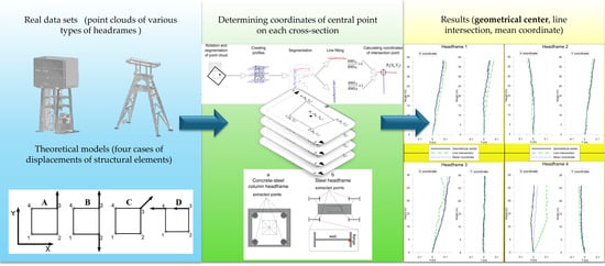
The subject of research was the influence of calculation methodology on values obtained for deflections of slender engineering structures. The calculations were carried out in the MATLAB environment [26] using proprietary data processing algorithms that automated most of the calculations. Theoretical research was carried out using virtual models of objects that consisted of four supports and were subject to deformation of varying degrees. Testing and validation of selected methods for determining the course of the main axis of a building were carried out on models of real engineering structures created on the basis of measurements made using terrestrial laser scanning (TLS) technology.

A special case considered in this article is shaft towers (headframes), which, as slender objects (symmetrical or asymmetrical), are also subject to dynamic impacts resulting from the movement of hoisting devices. This factor may add to the deformation processes that already result from the location of the shaft tower in a mining area.

In the case of headframes (in accordance with Polish law, §542 of the Ordinance on detailed requirements for the operation of underground mining plants, Regulation of the Minister of Energy of 23 November 2016), deflection of the vertical axis should be analyzed and may not exceed the limit value of 1/500 of the tower height. However, regardless of the type of object, the key element, i.e., the main axis of the structure, remains an undefined parameter. In the case of classic objects with an axially symmetrical structure (e.g., industrial chimneys or cooling towers), such an axis is determined by determining the geometric centers of circular or elliptical cross-sections, assuming that the load-bearing structure is contained within the shell. In the case of more complex structures (e.g., shaft towers), the definition of the main axis is not precise. Due to the many types of shaft towers (steel shaft trestles, concrete tower shafts, etc.), it is very difficult to define elements of analysis and select characteristic points of measurement.

2.1. Virtual Data Sets

Virtual spatial models were created taking into account the standard construction of the abovementioned slender objects. The created schemes are also compatible in construction with the objects on which subsequent testing and data validation were performed. The models are characterized by a construction system consisting of four supports or load-bearing elements arranged symmetrically. In order to investigate the movement of the main axis of the object, depending on the calculation method, its supports were deformed in four variants, as shown in Figure 1. The structure change patterns presented in the research (A, B, C and D) are only theoretical model changes. Real changes will never be of exactly this nature or value. In fact, all elements (struts and foundation footings) are subject to greater or lesser changes, sometimes taking place in different directions. The causes of such deformations may be various: uneven land depressions caused by exploitation, uneven impact of the winding machine or changes in ground conditions near the foundations of the structure [27,28].

In each case, the corners of the lowest, “0”, profile had the following coordinates: 1 (0.0), 2 (1.0), 3 (1.1) and 4 (0.1). Then, by simulating changes in the geometry of the object in the next 100 cross-sections, located at different, specified heights, the coordinate values of the selected points were linearly changed. In order to determine differences in their position relative to the theoretical (undisturbed) position, the maximum value of changes in selected elements was set at 100%, which allowed the data to be presented in a dimensionless form.

In the first case, A, displacement of element 3 was simulated, changing the shape of the object from a square in cross-section to a rectangular trapezoid. In this instance, the change affected only the Y coordinate. In the second case, B, both elements 2 and 3 were deformed simultaneously, changing the shape from a square to an isosceles trapezoid. As with A, only the Y coordinates of the selected supports changed. The values of the changes for supports 2 and 3 were identical, while the directions of change were opposed. In the case of C, element 3 was again displaced, but the direction of change was inclined by 45 degrees relative to the X axis. In the case of D, elements 3 and 4 were subject to deformation, the direction of change being parallel to the X axis. Only in case A did the figure stop being symmetrical. In cases B and C, the figure maintained one axe of symmetry, while in case D, the figure maintained two axes of symmetry. This had visible consequences in the analysis of results.

The discussed theoretical analysis consisted of determining the location of the central point on the next 100 cross-sections in each case using three calculation methods: average coordinate, intersection of diagonals and geometric center. These methods are described in Section 2.3.

2.2. Real Data Sets

Tests verifying the theoretical assumptions of the proposed method were carried out on models in the form of point clouds representing four shaft towers. Two of these were concrete–steel column headframes (headframes 1 and 2) and two were steel A-shaped headframes (headframes 3 and 4). The first type is characterized by a load-bearing structure based on columns, with a shape similar to cylindrical (Figure 2a). The second type is characterized by a symmetrical arrangement of struts (made of I-beams) around the shaft pipe (Figure 2b).

Towers 1 and 2 are objects of similar dimensions. In the lower part of the structure, there are load-bearing columns, which are connected at a height of about 41 m by a solid structure covered with plate girders, forming the engine room building. The total height of the towers is 70 m and the analyzed column levels (Level 1) reach a height of 40 m.

Towers 3 and 4 are steel trestle-type towers (two struts) with a total height of 40 m. The struts are the main element of the load-bearing structure of this type of tower, so the analysis of their geometry is particularly important. The towers are made of steel I-beams with a large cross-section. At the level of the lower rope pulleys (about 30 m), the struts are rigidly connected to each other, forming the frame structure of the tower.

Terrestrial laser scanning technology was used to perform the required measurements. Two panoramic laser scanners were used for this purpose: a Faro S350 phase scanner (Figure 2a) and a Leica ScanStation C10 pulse scanner (Figure 2b). In addition, classical angular–linear measurements and measurements using GNSS technology were performed. Topcon Hiper V GNSS devices in static mode were used to determine the coordinates of field points within the shaft areas. During the alignment process, point accuracies ranging from ±(0.002 to 0.004) mm were achieved. Based on the points established using GNSS technology, the coordinates of the measurement targets were determined using a Topcon OS103 total station. Integration of measurements from various instruments made it possible to increase the accuracy of the scan registration process and the georeferencing of measurements. Leica Cyclone 9.1 software was used to record the scans. In each case, the main method of combining the scans was registration with the use of targets (checkerboards and spheres). In order to increase precision, a cloud-to-cloud registration process was also carried out, which supplemented the registration for targets. Details of the measurement and registration of point clouds on objects are presented in

Table 1. Basic information about registered point clouds.

	Headframe 1	Headframe 2	Headframe 3	Headframe 4
Point cloud view
Scanner	Focus S 350	Focus S 350	Leica ScanStation C10	Leica ScanStation C10
Number of scan positions	4	6	4	5
Registration mean absolute error [mm]	±10	±7	±4	±5

. The mean absolute error is determined by taking into account the lengths of spatial vectors between the same targets for a pair of registered scans and those resulting from the process of fitting point clouds using the Iterative Closest Point (ICP) method.

2.3. Methodology for Determining Central Points of Supports

Point clouds exported after the registration and filtering process [29] were the basis for a semi-automatic analysis of the inclination of the structures. The MATLAB environment [26], in which the entire procedure was programmed, was used for this purpose. The first stage was the manual selection of load-bearing elements of the point cloud: from each object, those fragments of the cloud were extracted. They represented the struts of the tower structure. Then, the algorithm used the selected elements to generate horizontal profiles with a fixed slice width and a fixed sampling pitch (distance between profiles). The width of the profile was set at 0.05 m and the resolution of data sampling at 0.10 m. This allowed the creation of a quasi-continuous picture of changes in the axis of the structure. On each of the cross-sections, a characteristic point was automatically determined, whose coordinates were identified with the coordinates of the support at this level and used in the analysis of the geometry of the object’s axis (Figure 3).

In the case of shaft towers with cylindrical struts (Figure 3a), the Circle_fit function was used. This algorithm was made available in the MATLAB environment by Izhak Bucher and is an extension of the 1991 code for fitting a circle into a set of points [30]. It uses the method of least squares (LSM) to minimize deviations between the determined radius and the distances from the point to the center of the circle as determined by the algorithm. This is one of the simpler methods of fitting and therefore allows for high computational speed, but has the disadvantage of the possibility of radius determination errors in the cases where points are located close to one another [31]. The method is based on the classic equation of a circle, in which the squares of deviations are minimized by solving the following equation:

$$F_1\left(a, \mathrm{b}, R\right)=\sum _{i=1}^n{{\left[\right(x_i-\mathrm{a})}^2+{{(y}_i-\mathrm{b})}^2-R^2]}^2=\sum _{i=1}^n{\left(z_i+B{x}_i+C{y}_i+D\right)}^2$$

where: $z_i=x_i^2+y_i^2$, $B=-2a$, $C=-2b$ and $D=a^2+b^2-R^2$, $(a, b)$—plane coordinates of the center of the designated circle, and R—radius of the circle.

Due to the imperfection of the filtration process, which in some cases left points on the cross-sections that did not fit the circle equation, the algorithm was supplemented with a fragment of code. An iteratively repeated circle-fitting procedure was used, in which an outlier was the point for which the limit value (difference in distance from the designated center in relation to the radius) was the largest. Iterations end when the arbitrary limit value is met. In the tests, this value was set at ±0.01 m.

In order to estimate the accuracy of the location of the designated center point of the circle ($m_C$), the RMS error of the set of residuals was calculated according to the following formula:

$$m_C=\sqrt{\frac{{\sum }_{i=1}^n{\left(d_i-R\right)}^2}{n}}$$

where: R—radius of the designated circle, d_i—distance of the i-th point from the center of the circle:

$$d_i=\sqrt{{\left(x_i-x_C\right)}^2{+\left(y_i-y_C\right)}^2}$$

and n—number of circle points.

In the case of steel towers with braces made of I-beams (Figure 3b), the procedure for determining the characteristic points was carried out as presented in Figure 4.

In the first stage, the algorithm rotates the point cloud so as to situate the object parallel to the axis of the coordinate system (and save the value of the rotation angle). In the next stage, two groups of points with similar values of the normal direction are selected from the point clouds of the I-beam fragment, into which the line is fitted (the v parameter defines whether linear regression is used on the X or Y coordinate). In the last stage, the coordinates of the line intersection point are calculated and the approximate accuracy of this determination ($m_C$) is estimated as the RMS error using the following formulae:

$${RMS}_X=\sqrt{\frac{{\sum }_{i=1}^n{(X_i-X_{śr})}^2}{ n}}, {RMS}_Y=\sqrt{\frac{{\sum }_{i=1}^n{(Y_i-Y_{śr})}^2}{ n}}$$

$$m_C=\pm \sqrt{{RMS}_X^2+{RMS}_Y^2},$$

where: ${RMS}_X, {RMS}_Y$—RMS error along the X and Y axes and n—number of points in the set.

Based on the coordinates of characteristic points determined in this way, the coordinates of the central point for each analyzed level were calculated using three selected methods. The estimated error in the location of the profile center points was determined from the dependence:

$$m_{XP}=\pm \sqrt{\frac{{\sum }_1^n{RMS}_{Xi}^2}{n}}, m_{YP}=\pm \sqrt{\frac{{\sum }_1^n{RMS}_{Yi}^2}{n}},$$

$$m_{2D}=\pm \sqrt{m_{XP}^2+m_{YP}^2} \mathrm{or} m_{2D}=\pm \sqrt{\frac{{\sum }_1^n{m}_{Ci}^2}{n}},$$

where: ${m_{Ci},m}_{XP}{, m}_{YP},m_{2D}$—average errors of determining the location of the central point (center of the circle, along the X, Y and linear axes) and $n$—number of supports.

2.4. Methods of Calculating the Center Points of the Section

For each of the analyzed objects (virtual models and real buildings), the course of the main axis of the structure was calculated based on the central points generated for each cross-section. The location of the central points was determined using three selected calculation methods.

The first method of determining the location of the main axis of the object, called “Mean coordinate” (MC), consisted of determining the coordinates of the central point of each cross-section by averaging the coordinates of the object’s load-bearing elements (Figure 5a) on successive cross-sections. The average coordinate of each profile was determined from the formulae:

$$X_{Śr}=\frac{{\sum }_1^n{X}_i}{n} \mathrm{o}\mathrm{r} Y_{Śr}=\frac{{\sum }_1^n{Y}_i}{n}$$

where: $X_{Śr},Y_{Śr}$—center point coordinates, $X_i,Y_i$—coordinates of the object elements and n—number of object elements.

The second method, “Line intersection” (LI), was based on determining the central point from the intersection of the object’s diagonals (Figure 5b). In this method, by determining the coefficients of the equation of the lines (a,b) passing through the opposite elements of the object (points 1–3 and 2–4), it was possible to determine the point of intersection:

$$X_P=\frac{b_2-b_1}{a_1-a_2} \mathrm{o}\mathrm{r} Y_P=\frac{{a_1·(b}_2-b_1)}{a_1-a_2}+b_1$$

where: $X_P{, Y}_P$—center point coordinates and $a_1,a_2, b_1,b_2$—parameters of straight lines containing diagonals of the object.

The third method, “Geometric center” (GC), consisted of identifying the central point of the cross-section of the object as the geometric center of the figure determined by four vertices. This method uses the “polygeom” algorithm provided by H.J. Sommer III in the MATLAB community [32]. This algorithm is used to determine the geometric parameters of a polygon such as perimeter, surface area, geometric center and moments of inertia, and is based on the method of determining geometric parameters proposed by Paul Bourke in 1988. Bourke showed that for closed polygons with non-intersecting edges (Figure 5c), the coordinates of the center of gravity can be determined from the formulae:

$$X_{Sg}=\frac{{\sum }_{i=0}^{n-1}(x_i+x_{i+1})·(x_i{·y}_{i+1}-x_{i+1}·y_i)}{6A}$$

$$Y_{Sg}=\frac{{\sum }_{i=0}^{n-1}(y_i+y_{i+1})·(x_i{·y}_{i+1}-x_{i+1}·y_i)}{6A}$$

where: $X_{Sg}{, Y}_{Sg}$—coordinates of the geometric center and $x_i{,y}_i$—coordinates of the polygon’s vertices,

$$A=\frac{{\sum }_{i=0}^{n-1}(x_i·y_{i+1}-x_{i+1}·y_i)}{2}$$

These analyses allow one to determine in a semi-automatic way the straightness and verticality of the main axis of a slender object and to estimate the accuracy of its determination.

3. Results

3.1. Results for Virtual Data Sets

Based on the algorithms for determining the central point of a profile (MC, LI and GC) described in Section 2.4, the course of the main axis of the analyzed object was calculated in four different simulated cases (A, B, C and D). The following diagrams (Figure 6) show the determined changes in the position of the central point for the simulated displacements of the structure’s load-bearing elements.

The change simulated in example A caused a change in the main axis of the object. Depending on the method of determining the coordinates of the central point, this resulted in a change in only one coordinate (according to the MC algorithm) or in both coordinates of the point (according to the LI and GC algorithms). The displacement in the direction of the Y axis was similar in value and direction regardless of method. On the other hand, displacement along the X axis (perpendicular to the displacement of the element) was found to vary. The values of the X coordinate of the central point as determined by the MC method do not change, while the LI method shows a decrease in values and the GC method shows a slight increase.

The change simulated in example B involved the displacement of two base elements of the object (elements 2 and 3). This type of deformation transformed the original figure into an isosceles trapezoid. Changing the Y coordinate of the two bases of the object caused the coordinates of the central point (object axis) to move along the X axis. The Y coordinate of the central point calculated with each method shows no variation. The X coordinate of the center of the object calculated with the MC method does not change, and with the LI method a slight increase in value is visible, while with the GC method a decrease is visible.

The change simulated in example C increased the value of both coordinates of one base symmetrically. This type of deformation transformed the shape from symmetrical to asymmetrical. Changing both coordinates of one of the bases of the object, depending on the method of determining the coordinates of the central point, either did not change its coordinates (LI algorithm) or caused displacement of the coordinates of the central point (object axis) along both the X and Y axes (MC and GC algorithms). The displacement determined by the MC algorithm has a smaller value than that determined by the geometric GC method. The direction of change is preserved.

The change simulated in example D involved the displacement of two elements of the base of the object. This type of deformation resulted in the transformation of the object from a square to a rhombus, thus maintaining the axes of symmetry of the object. According to each of the three methods, this resulted in the same displacement of the central point.

3.2. Results for Real Data Sets

Despite the filtration processes carried out, there were results that differed from others. They influenced the determined coordinates of the structure’s axial points, but their number was small and due to their chaotic nature, they were easy to select. The process of determining the course of the axis was also carried out for the tested shaft towers. Graphs showing the course of the axes of each of the tested objects can be seen in Figure 7.

The results of the analysis of the course of the main axis carried out on the shaft towers are quite surprising. For tower shaft towers nos. 1 and 2, the results of the analysis carried out with different algorithms were convergent, while for shaft towers with trestle construction (3 and 4), significant differences were visible for the X coordinate. The results of the MC method were in most cases similar to those of the GC method, but the results of the LI method were particularly divergent, most notably in the case of tower no. 4.

These results confirm theoretical considerations. Differences in the assessment of the verticality of the current state of the object are noticeable, significantly changing the conclusions of the interpretation. In accordance with the conclusions from the analysis of determining the location of the central point, the geometric center was selected as the most reliable method in terms of the obtained results.

4. Discussion

The analyses and theoretical modeling performed above demonstrate the importance of a problem that is often overlooked in studies of the geometric state of slender and elongated objects. In the previously cited articles, e.g., [6,7], researchers analyze deflections of structures with a circular cross-section. Determining the center of such a construction is unambiguous. However, if we are to describe a change in the geometry of objects with a more complex structure (having many edges or an asymmetric shape), the need to adopt an appropriate computational strategy assumes great importance. Unfortunately, this issue is very poorly described in the literature and case studies largely confine themselves to consideration of changes detected on the outer surfaces of objects or to theoretical calculations described by FEM models [3,4,5,33].

The solutions proposed by the authors are adapted to the shape of the objects for which they were formulated. In the case of objects with a different, more or less diverse structure, separate tests will need to be carried out. The algorithm proposed by the authors, based on the geometric center, seems resistant to changes in the structure of the object, giving the most reliable location of the centers of cross-sections. However, to be sure, appropriate tests should be carried out in the future.

In the worst case (for asymmetric, single-stay towers), discrepancies in determining the course of the vertical axis of the structure were shown to be about 0.12 m—a finding that has significant implications for the process of controlling the stability and geometric invariance of a structure as a function of time. In cases where differing or arbitrary means of calculating this axis are adopted in different research periods, false conclusions may be reached, even on the basis of accurate observational data. This also relates directly, among other things, to the process of admitting such tower structures for further operation. For example, in Polish law, the inclination of such structures cannot be greater than 1/500 of the height of the building. This means that, if we take into account the average height of such shaft towers (approximately 50 m), any deflection of more than 0.1 m must be regarded as threatening the legal functioning of the facility. In light of the extreme values of the discrepancies in the positions of the axes determined above, it is evident that the correctness/abnormality of the geometric state of a slender object can be incorrectly assessed.

5. Conclusions

The adoption of an appropriate calculation strategy is of key importance for obtaining correct and reliable information about the course of the axis of a structure or object under analysis. The results of this study, based on three methods of calculating the axial point (geometric center, mean coordinate and intersection of construction lines of the cross-section), indicate significant discrepancies in determining the vertices of the virtual longitudinal axis of an object, especially one that is not axisymmetric. This is confirmed by both theoretical considerations and actual results based on experiments related to shaft towers of various shapes.

Therefore, the clear conclusion is that we should always perform periodic analyses using the same method, even if the computational strategy has not been analyzed. This will at least allow us to determine periodic changes correctly, but we will still of course be burdened with incorrect diagnosis of the state of total changes, identified with deviation from the vertical line. The correctness of this total determination can only be ensured by the selection of the correct computational strategy—geometric center (GC). This is what the authors of the article propose through the considerations and experiments presented above. Our analysis is particularly important in the case of the installation in facilities of devices, such as hoisting devices and elevators, that are especially sensitive to the maintenance of verticality. It should be emphasized that combining methods and periodic analyses using different strategies (e.g., when such analyses are performed by different research teams) is the worst possible solution, as it offers no guarantee of correct assessment of periodic—still less, total—changes.