Review

Recent Phenomenal and Investigational Subsurface Landslide Monitoring Techniques: A Mixed Review

by
Kyrillos M. P. Ebrahim
1,2,
Sherif M. M. H. Gomaa
1,2,*,
Tarek Zayed
1 and
Ghasan Alfalah
3
1
Department of Building and Real Estate, Faculty of Construction and Environment, The Hong Kong Polytechnic University, Hung Hom, Kowloon, Hong Kong SAR 999077, China
2
Structural Engineering Department, Faculty of Engineering, Mansoura University, Mansoura 35516, Egypt
3
Department of Architecture and Building Sciences, King Saud University, Riyadh 145111, Saudi Arabia
*
Author to whom correspondence should be addressed.
Remote Sens. 2024, 16(2), 385; https://doi.org/10.3390/rs16020385
Submission received: 24 November 2023 / Revised: 3 January 2024 / Accepted: 8 January 2024 / Published: 18 January 2024

Abstract

:
Landslides are a common and challenging geohazard that may be caused by earthquakes, rainfall, or manmade activity. Various monitoring strategies are used in order to safeguard populations at risk from landslides. This task frequently depends on the utilization of remote sensing methods, which include the observation of Earth from space, laser scanning, and ground-based interferometry. In recent years, there have been notable advancements in technologies utilized for monitoring landslides. The literature lacks a comprehensive study of subsurface monitoring systems using a mixed review approach that combines systematic and scientometric methods. In this study, scientometric and systematic analysis was used to perform a mixed review. An in-depth analysis of existing research on landslide-monitoring techniques was conducted. Surface-monitoring methods for large-scale landslides are given first. Next, local-scale landslide subsurface monitoring methods (movement, forces and stresses, water, temperature, and warning signs) were examined. Next, data-gathering techniques are shown. Finally, the physical modeling and prototype field systems are highlighted. Consequently, key findings about landslide monitoring are reviewed. While the monitoring technique selection is mainly controlled by the initial conditions of the case study, the superior monitoring technique is determined by the measurement accuracy, spatiotemporal resolution, measuring range, cost, durability, and applicability for field deployment. Finally, research suggestions are proposed, where developing a superior distributed subsurface monitoring system for wide-area monitoring is still challenging. Interpolating the complex nonlinear relationship between subsurface monitoring readings is a clear gap to overcome. Warning sign systems are still under development.

1. Introduction

The practice of landslide monitoring is the systematic observation and collection of data to enhance the understanding and analysis of this geological event. Any effective monitoring methodology should include the following goals: consistent and systematic data collection, the use of appropriate equipment, accurate timing of measurements, and the use of proper analytic techniques (i.e., how to interpret the collected data). These goals can respond to the following questions: (1) what has to be monitored (such as displacement, stress, and pore water pressure), (2) the number of devices to be utilized, and (3) the frequency and data collection methods. These goals and inquiries may be used to establish the budget, resources, planning, and monitoring system [1].
Geotechnical investigations have been conducted for years to discover the stability conditions of slopes under various geological and environmental circumstances [2,3]. To answer the first aforementioned question, landslide monitoring is used to track and measure slope stability parameters, such as ground movement (surface movement, subsurface movement, heights, and cracks), subsurface water conditions (depth of water table, pore water pressure, soil suction, and soil moisture), and climatic parameters (rainfall, snowfall, temperature, and humidity). These factors can subsequently be used in landslide prediction approaches, which were not the focus of this work [4,5]. The number, type, and location of sensors are determined by the local geology, subsurface conditions, and landslide area in answer to the second question [6]. Concerning the third question, comprehending the geographical and temporal distributions of these factors is critical for realizing landslide dynamics and controlling the associated risk [7].
Determining the most effective monitoring system requires a thorough understanding of the reasons that generate events (initial conditions). For instance, the use of tilt measurement may not be suitable for translational landslides or slow-moving landslides since the occurrence of tilting is improbable under such conditions. Similarly, when deep soil underneath an installation site becomes saturated, it might lead to landslides, which can damage topsoil moisture sensors [8]. Another example is if the effective rainfall value is the cumulative value of one day, then collecting data at 15 min intervals may not be necessary [1]. Landslides are classified as shallow or deep-seated based on the depth of the slip surface. Both of these types of landslides have distinct features and produce varying degrees of damage. As a result, defining the type of landslide and estimating the potential risk of a prospective landslide by measuring the depth of the sliding surface are both necessary [1]. The monitoring of landslides is divided into phenomena, investigation, and performance categories. The change in the slope over time in a particular geologic location is monitored using phenomena. To ascertain the temporal and physical parameters of an identified landslide, investigation monitoring is performed. A stabilizing system that is already in place can be evaluated for efficacy via performance monitoring [1].
Monitoring systems can be classified into surface and subsurface techniques [9]. The former cannot follow internal changes, but the latter can. Thus, this research focused mostly on subsurface monitoring approaches, where the optimal criteria for a monitoring system, according to the literature, should have the following features: provide real-time data; high sensitivity; high spatiotemporal resolution; cost-effectiveness; low power consumption; reliability; scalability; not affected by signal noise, such as temperature effects; limit the uncertainty caused by missing data; and be suitable for both shallow and deep landslides, as well as harsh environment conditions (i.e., the device should be coated) [10,11,12].
Both scientometric and systematic methodologies are covered in this paper. This paper is organized as follows: The research technique is presented in Section 2. The scientometric analysis is highlighted in Section 3. The systematic analysis is emphasized in Section 4, which is divided into four subsections: surface displacement, subsurface monitoring, wireless sensing networks, and physical and prototype systems. Section 5 lists the research gaps and future directions. Section 6 presents the conclusion and future recommendations.
According to the author’s knowledge and available data, Table 1 shows various review studies that investigated landslide-monitoring techniques. Many of them focused on a specific methodology and approach. There is a lack of review publications on subsurface monitoring techniques. Scientometric analysis has rarely been used. As a result, this study’s uniqueness may be summarized as follows:
(1)
A mixed scientometric and systematic review is presented.
(2)
All existing subsurface-monitoring technologies (movement, forces and stresses, groundwater, temperature, and warning signs) were comprehensively addressed in this study.
(3)
A deep illustration of the data-transferring techniques is included (i.e., manual, wiring, wireless).
(4)
A detailed demonstration of the adopted physical laboratory and field-monitoring systems is presented.
(5)
This article presents the most recent research up until 2023.
This study examined the progression from one approach to another through a macroscopic view based on the technology utilized and the initial conditions, followed by a microscopic demonstration of the different system characteristics.

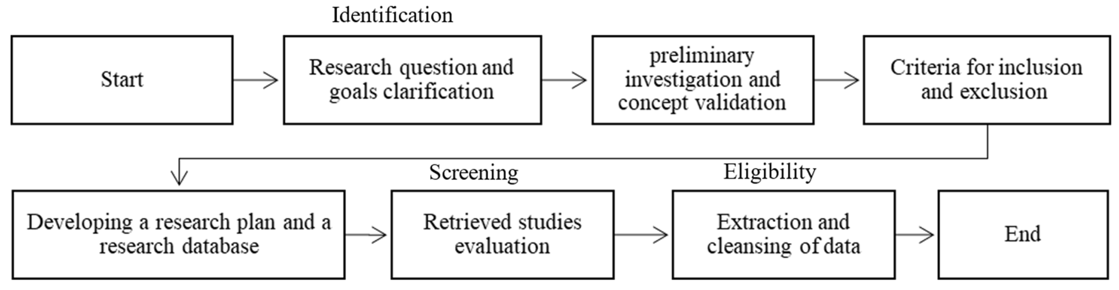
2. Research Methodology

A mixed review strategy was employed in this study, which consisted of scientometric and systematic techniques. The methodology is provided to help researchers improve systematic review reporting through the use of scientometric analysis. Furthermore, it highlights the complexity of conducting manual searches on database engines [21,22,23,24].
Identifying, screening, and qualifying are the three main steps of a systematic review, as shown in Figure 1. The steps involved in doing scientometric analysis are shown in Figure 2. These steps typically include collecting bibliometric data, exporting it to the suitable software, evaluating it, and finally, discussing the findings.

2.1. Identification Process

Geology, engineering, environmental science, ecology, meteorology, atmospheric science, geochemistry and geophysics, physical science, and water resources are some of the aspects used to study landslides [24]. Furthermore, as shown in Zou and Zheng’s [24] keyword mapping, landslides have a large number of linked terms. As a consequence, the research method began by extracting important studies about landslides from the author’s perspective. In this section, keywords, search databases, and inclusion and exclusion criteria were utilized to filter the papers acquired.

2.2. Selection of Database and Keywords

It is advisable to select numerous databases in a systematic review to obtain and review a thorough selection of relevant publications. Scopus, Web of Science, and Google Scholar are the three most often used databases in engineering research. Scopus and Web of Science are also compatible with modern scientific mapping programs, such as VOSviewer. In this study, we only used Scopus and Web of Science as preliminary search database sources for landslide monitoring, although Google Scholar was also employed in the snowballing approach. Following the selection of a search database, relevant keywords were chosen, namely, “landslide monitoring”, to take into account all accessible datasets for monitoring approaches.

2.3. Inclusion and Exclusion Criteria

In any systematic review, inclusion and exclusion are crucial for limiting search results and focusing on the most relevant ones. This research used the following criteria: (1) research focusing on subsurface landslide monitoring, (2) studies published between 2000 and 2023, (3) articles published in peer-reviewed journals, and (4) studies published as articles and review submissions. The exclusion criteria were as follows: (1) papers published in a language other than English, (2) studies with no full text accessible, (3) manuscripts published in a subject area other than engineering, and (4) publications published in a source type other than a journal.

2.4. Screening and Evaluation of Collected Articles

As of May 2023, the Scopus and Web of Science databases revealed a total of 173 and 98 articles, respectively. The selected publications were then evaluated and assessed using the systematic reviews and meta-analyses (PRISMA) process (see Figure 3) [26]. Following this method, 143 papers were eliminated because they were duplicated, irrelevant, or did not have a complete text accessible. After reviewing the whole texts of each included article, 128 articles met the inclusion criteria. The backward and forward snowballing methods were then used to find more studies that were not found using Scopus or Web of Science searches [27]. In addition to the manual search, this search method yielded 26 more relevant articles, for a total of 154 articles suitable for inclusion.

3. Scientometric Analysis

The scientometric study was conducted with the open-source VOSviewer software application version 1.6.20 [25]. This scientometric review was used to provide citation and co-authorship analyses of nations, organizations, authors, and keywords involved in the study topic, as shown in the following subsections. The resulting maps, networks, and analyses (i.e., the VOS output; please refer to Section 3.1, Section 3.2, Section 3.3, Section 3.4 and Section 3.5) highlight the link between these many aspects, whereas tables were mainly utilized to illustrate the statistics associated with these network maps. VOSviewer software was used to assess the 154 articles retrieved via snowballing and manual searching. The primary goal of scientometric analysis is to guarantee that the findings are relevant enough to be included in a systematic review.

3.1. Landslide Monitoring Annual Publications

Figure 4 depicts the overall number of landslide-monitoring-related papers published each year. From 2000 to 2016, the average yearly publishing rate was approximately two articles. Between 2017 and 2023 (until May 2023), the publishing rate increased significantly to record an average annual publishing rate of approximately 15 articles. The figure’s second-degree polynomial trend line (refer to the trend equation presented in Figure 4) depicts how landslide monitoring has evolved. This trend is not surprising considering the world’s growing concern over the loss of human life, property, and economic resources due to landslides.

3.2. Top Journals Contributing to Landslide Monitoring

The VOSviewer tool can now highlight the journals that frequently publish landslide-monitoring articles. As a consequence, this will help researchers choose a reputable journal in this field. When utilizing the VOSviewer program, the author employed two thresholds: a source has to include at least five documents and at least 10 citations. “Sources” were employed as the unit of analysis, and “bibliographic coupling” was the type of analysis. As a result, 7 journals out of 62 hit the threshold (Figure 5). In Figure 5, the node size illustrates the influence of journals as weighted by the number of citations. The overall link strength of a journal represents the number of links it has with other journals [25]. Engineering Geology was the most widely published and cited journal and had 449 citations and 12 publications.

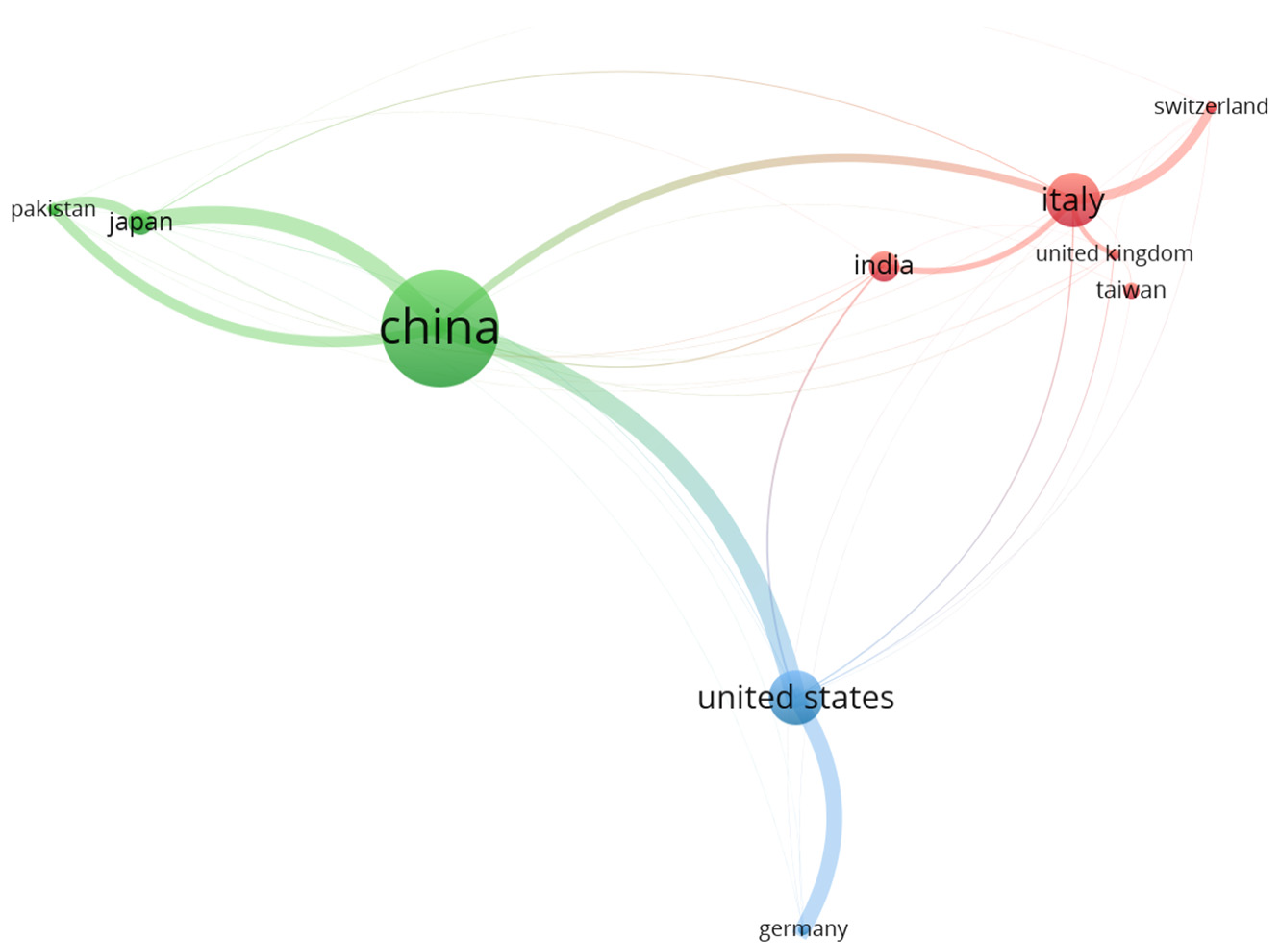
3.3. Active Nations and Institutes in Landslide Monitoring

Understanding the scientific collaboration network makes it simpler to identify top laboratories, organizations, and nations. Furthermore, academic and industry practitioners seeking innovative landslide solutions should be aware of the cooperation network of nations investing more in this field. The aforementioned criteria were utilized, using “countries” as the unit of analysis and “bibliographic coupling” as a type of analysis. Only 10 of the 43 nations met the criterion. Figure 6 depicts the most frequently publishing nations, with China, the United States, and Italy having the most publications globally, with 50, 23, and 23 articles, respectively. Table 2 reports the top five institutions involved in landslide monitoring by using “bibliometric coupling” as the kind of analysis and “organization” as the unit of analysis. With five papers and 76 citations, the most frequently contributing institute was the School of Civil Engineering of Chongqing University, China.

3.4. Active Scholars and Article Co-Citation Analysis in Landslide Monitoring

An author’s total number of publications and citations on a certain topic can be used to calculate their influence on that topic. The top five authors based on the number of publications and citations were assembled using Excel Microsoft 365 software, as shown in Table 3. To solve the issue of older research obtaining more citations than more recent research, a normalized citation metric was also utilized in this study. The number of citations in an article was normalized by dividing the number of citations by the average number of citations in all publications published that year [25]. As a result, Table 4 lists the top five publications based on normalized citations.

3.5. Co-Occurrence Mapping of Keywords in Landslide Prediction

By selecting “co-occurrence” as the kind of analysis and “all keywords” as the unit of analysis, VOSviewer software version 1.6.20 can identify the most frequently used keywords (i.e., the keywords used in literature). In this analysis, the author fixed the minimum number of occurrences at 10; only 17 keywords out of 1050 matched this requirement. The size of a keyword node correlates to its occurrence frequency. To illustrate, the most commonly used terms were “landslides” and “landslide monitoring,” which had the largest node sizes of any keywords. Figure 7 highlights that there were three distinct clusters: green, blue, and red. The blue clusters show monitoring related to rainfall and soil moisture; the red clusters highlight keywords linked to monitoring sensors and wireless networks; and the green clusters highlight subsurface displacement monitoring systems, such as optical fiber techniques.

4. Systematic Review of Monitoring Techniques

Landslide monitoring can be divided into two main categories: (1) surface- and (2) subsurface-monitoring techniques. In the following sections, both surface and subsurface monitoring are illustrated in detail. Figure 8 lists the surface-monitoring techniques, while Figure 9 presents the subsurface-monitoring process, including the testing procedure and data transfer mechanism. This paper first discusses the existing surface-monitoring approaches (refer to Figure 8 and Section 4.1), which have been well evaluated in the literature (refer to Table 1). Then, an in-depth investigation of subsurface procedures (such as movement, forces and stresses, water and temperature, and warning techniques) is presented. The warning approaches are subsurface monitoring devices that simply give a warning indication and no quantifiable data. The subsurface monitoring system is consistent with data-collection challenges, as well as prototype and physical modeling systems that are assessed to present a complete picture of such a topic (see Figure 9).

4.1. Surface Displacements

Surface displacement can be measured using various techniques, such as total stations, global positioning system (GPS) [38], robotized total station (RTS) [39], light detection and ranging (LiDAR) [16], synthetic aperture radar (SAR), interferometric synthetic aperture radar (InSAR) [40], persistent scatterer interferometry (PS-InSAR) [41], differential synthetic aperture radar (SAR) interferometry (DInSAR) [42], ground-based InSAR (GB-InSAR) [43], terrestrial laser scanning [44], global navigation satellite system (GNSS) [19], aerial photography [45], and satellite remote sensing techniques [46]. These techniques can only provide information about ground movements and are useful for wide-area surveillance. However, such instruments cannot determine the subsurface physical mechanism of landslides [14,15,16,19,20,47,48].
The GPS technique works on the basis that GPS satellites give navigation positioning signals for space resection measurement, hence calculating the 3D coordinate of the measuring point. However, high-power radio-transmitting stations and high-voltage transmission lines have a significant impact on GPS [9]. Furthermore, one GPS monitoring site costs approximately USD 6000 for a single device [49]. A robotized total station (RTS) is beneficial for distributing information about the present landslide condition and can give near real-time data, such as the ADVICE system [50]. However, false alarms owing to data inconsistencies caused by instrument faults, physical changes at the measurement location, and/or extremely local/shallow reactivations are always possible [50].
Remote sensing techniques (space-borne, aerial, and terrestrial surveys) can monitor broad regions without physical contact with the ground, though these technologies are expensive, have low resolution, and have difficulty collecting real-time data [7]. Although InSAR offers a better spatial resolution than GPS, it is hampered by atmospheric delay. Although PS-InSAR, which is an advanced radar interferometric measurement type that is representative of DInSAR, offers good accuracy, it is impacted by shadows and dense vegetation [9]. In satellite- and airborne-based SAR applications, the technique of differential synthetic aperture radar (SAR) interferometry (DInSAR) has been utilized to monitor vast regions of longer-distance landslides. DInSAR-based systems estimate displacements in millimeters by measuring phase changes between pairs of ground pictures acquired at various time intervals. The drawbacks are that the monitoring time intervals are excessive, ranging from hours (airborne) to weeks (satellite), and that daily or hourly monitoring is costly. Ground-based SAR (GB-InSAR), which is utilized over ranges ranging from a few hundred meters to a few kilometers, was created to alleviate the aforementioned difficulties. However, when a large bandwidth signal (for a high resolution in the range direction) is employed, a costly instrument is required [51,52]. The 3D laser scanning method has the added advantage of rapidly collecting (every 5 min) field deformation topography data with high accuracy and resolution [53]. However, the performance of a laser-light-based device is also influenced by weather conditions, such as severe fog or snow/rain [51]. By employing radio waves to scan a large area of the slope and provide temporal pictures, radar devices can track the movement of the slope. Nevertheless, there are drawbacks to using radar systems, such as the inability to monitor the slope in the event of snowfall or rain or when the line of sight (LoS) between the scanning device and the target slope is blocked. The technology is also useless for providing real-time warnings of sudden movements (i.e., seconds) since it takes several minutes to hours to scan the slope and interpret the photos to detect changes in the slope state [28].
A global navigation satellite system (GNSS) has been suggested to eliminate the requirement for line of sight (LOS) and to offer high-precision 3D monitoring. However, this technology has a significant maintenance cost and time requirements, as well as the presence of a single point of failure [54]. LiDAR-derived digital elevation models (DEMs) can quantify minor displacements across broad regions. Nevertheless, choosing an appropriate DEM resolution (i.e., pixel size, grid resolution, grid size) for constructing susceptibility maps is sometimes difficult since the scale of observation influences the evaluation, results, and interpretation [55].
The gradual degradation of slope stability generates landslides, and the sliding surface plays a vital role in landslide evolution. To illustrate, the landslide initiation is generated from the subsurface deep layers: only when the slope mass changes sufficiently can the slope surface deform macroscopically [56]. Surface monitoring systems may detect millimeter-scale deformation and can monitor wide regions with good spatial resolution and 3D capabilities, which is appropriate for landslide susceptibility, vulnerability, and risk maps for planning. The considerable time these systems need to spend returning to the same location, however, prevents these systems from offering real-time monitoring [57], and is not adequate for rapid landslides [29,58]. Therefore, there is a need for improvements in the small-scale subsurface monitoring of landslides [59,60]. To demonstrate this, Mucchi et al. [54] compared wireless sensor networks for ground instability monitoring (Wi-GIM) with RTSs and GB-InSAR to illuminate the fact that such sensor networks suffer from durability, precision, environmental impact, and maximum measuring range issues, and thus, further improvement is needed, as presented in Table 5. Surface displacement techniques are widely discussed in the literature (refer to Table 1), while this study mainly focused on subsurface monitoring systems.

4.2. Subsurface Monitoring

Landslide deep displacement monitoring, where landslide initiation begins, is important for early warning forecasting and stability assessment [4,5,9]. In addition to displacement monitoring, subsurface monitoring techniques provide the added benefit of tracking internal forces, stress, moisture content, and temperature changes. Furthermore, such methods can provide early signs for emergencies.

4.2.1. Movement-Monitoring Devices
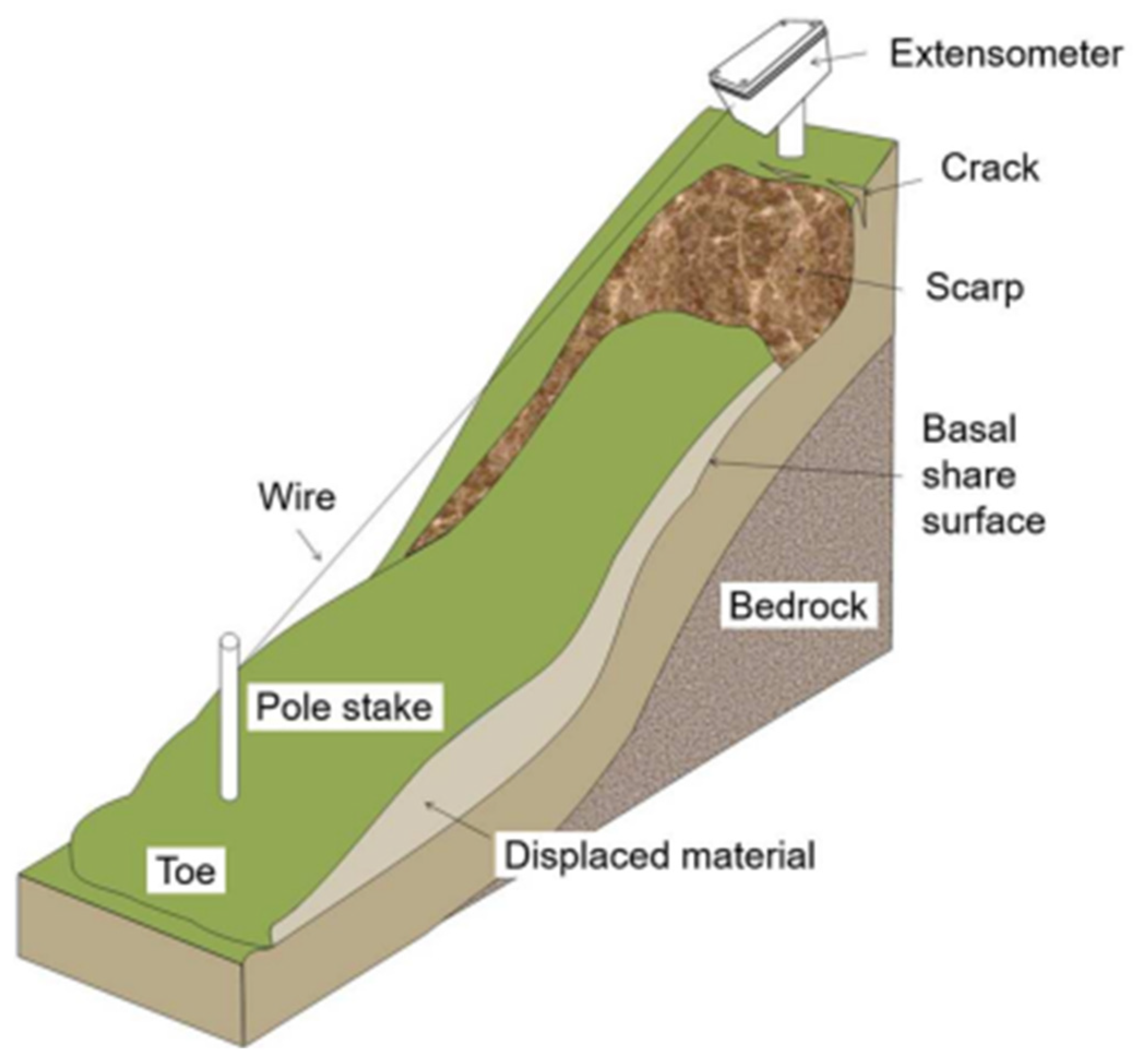
Extensometer Device

A conventional wire extensometer can provide a continual check of surface movement that may lead to a landslide. During emergencies, data can be obtained at regular intervals of 1–3 h, yet during routine situations, measurement intervals are 6 h. However, to obtain meaningful readings, the wire must be continually tensioned [2]. The quantity and rate of movement are measured and calculated manually within a centimeter range. However, key events might be missed if measurements are not obtained on time. To overcome the aforementioned issues, potentiometric extensometers detect displacement using a variable resistance mechanism, where a movable arm makes electrical contact along a fixed resistance strip. This type has the advantage that the wiring can be buried [61]. Crawford et al. [62] used a cable-extension transducer, which is a stainless-steel cable connected to a potentiometer housed in a protective casing, where the voltage output is then transformed to a linear absolute displacement. Fibreglass extensometers were initially placed (drilled horizontally in boreholes) in the S landslide to provide more precise data [2]. This type of extensometer is suited for rock slide applications since it can detect movement in the millimeter range [2]. Setiono et al. [63] created optical-based wire extensometers with an optical rotary encoder to count optical pulse signals and transform them into length units (refer to Figure 10). This approach offers a high resolution of 0.011 ± 0.0083 mm and a speed limit of approximately 36 mm/s.
Nevertheless, the wire extensometer has the drawback of collecting data at the landslide surface, making it hard to analyze the deep displacement distribution, and being overly expensive, costing approximately EUR 1000 for a single monitoring site [64]. Moreover, this technique is a single-point measuring technique and cannot provide distributed monitoring [8,65]. With technological advancement, wire extensometers may now deliver real-time and high-resolution measurements. Wire extensometers can be linked to particular data logging units and can be combined with other sensors for landslide dynamic analysis. While this technique is more suited for translational landslides, it can additionally be used in roto-translational landslides and has been validated in field experiments with land shifts ranging from 12 mm to 150 mm [63].

Inclinometers

Compared with extensometers, inclinometers have the benefit of measuring deep displacement with a spatial vertical resolution of 0.5–1 m [66,67]. Measurements are collected regularly by installing a single inclinometer into grooved vertical pipes installed in deep boreholes to analyze their deformation. Later investigations employed numerous analog inclinometers or a series of digital in-place inclinometers positioned at different depths inside these pipes for continuous measurement. Inclinometers, however, are difficult to install, laborious, lack sensitivity, and are vulnerable to environmental dangers [10,61]. Using an inclinometer to determine the precise location of sliding surfaces is limited by the spatial vertical resolution [68,69], especially when the shear band thickness is small [35]. Automating inclinometers is impractical because the wiring restricts the number of inclinometers that may be installed in a region, resulting in limited area spatial resolution [70]. This approach is impracticable for measuring significant lateral deflections for two reasons: the limited displacement range [9] and the high expense of guide casing (approximately 30 USD/m) [47] (600 USD/inclinometer) [71]. Electric-powered inclinometers are the most often used equipment for measuring subsurface displacements. However, in real applications, this technique (i.e., electric-powered inclinometers) suffers from limited stability and durability, poor resistance to electromagnetic interference, high gravity dependency, and significant signal loss for long-distance transmission [72].
Thus, inclinometers are appropriate for landslides that move very slowly to slowly [73] and have a thick shear bandwidth (refer to Figure 11), for which a lengthy monitoring interval and low spatial resolution would be sufficient. Intelligent monitoring for landslides has been widely studied [74]. Recently, numerous research studies have been conducted to overcome the inclination drawbacks by improving the spatiotemporal resolution, lowering the cost, giving real-time data, and enabling wireless data transmission.

Time Domain Reflectometry (TDR)

TDR is a relatively new method that, similar to radar, employs a coaxial cable and a cable tester (refer to Figure 11) [70,71]. A TDR device is made up of a TDR step pulse generator, an oscilloscope (or receiver), and a transmission line coupled to a multiplexer for multipoint and multifunction usage through various types of sensing waveguides [69,75]. An electrical pulse is sent down a coaxial cable that has been grouted into a borehole by the cable tester. The pulse is reflected when it encounters a crack or distortion in the cable. The reflection is represented by a “spike” in the cable signature. The relative magnitude and rate of displacement, as well as the position of the deformation zone, can be measured instantly and precisely [69]. Lin et al. [70] examined TDR behavior using laboratory and numerical simulations in an attempt to quantify TDR displacement. The main assumptions and findings can be summarized as follows: (1) TDR looks useless for quantifying shear displacement unless the shear mode is fixed (for example, if a sliding surface exists between soft soil and the bedrock layer). To fix the shear mode in the sensor cable, a hard, brittle grout with low tensile strength can be utilized. (2) The relationship between soil and grout stiffness has no effect on the TDR response. (3) Achieving high-strength grout is preferable because the sliding force required to kink the sensing cable is greater than the grout strength. Ho et al. [68] quantified the relationship between the horizontal displacement and reflection coefficients with an R2 of 0.93 through laboratory and field tests. Chung and Lin [69] used recent literature findings to construct a field prototype monitoring system with the following model characteristics: (1) water/cement ratio = 1 to improve the cable–grout–soil interface contact; (2) sand and gravel were suggested to be mixed into the grout cement when grout loss occurs; and (3) the spatial resolution was 5 cm, which was higher than that of conventional inclinometers and can determine the location of sliding surfaces at different depths. Chung and Lin [69] found that TDR can work with inclinometers (IN) to allow for more precise geological and mechanical modeling of a landslide, determining the amount and direction of shear deformation. In this context, placing TDR wires outside IN casings was considered for economic reasons [76]. Using a high-gravity centrifuge, Chung et al. [75,77] enhanced the applicability of TDR. A flexible coaxial wire was modified to increase its sensitivity for detecting small-scale shear displacement (0.5 mm).
Figure 11. TDR deformation mechanism and affecting factors “Reprinted/adapted with permission from Chung & Lin [69], Elsevier”.
Remotesensing 16 00385 g011
This approach, however, faces challenges when quantifying the amount of displacement [68,78]. This is because numerous factors influence displacement, including (1) cable resistance, (2) soil–grout–cable contact, and (3) interaction and shear bandwidth. As a result, each cable has unique calibration measurement features. TDR is not suitable for multi-landslide failure zones [9]. TDR is not recommended for fast-flowing landslides or difficult-to-access steep slopes [29]. This method works best on rock slopes, and it is less effective on soft soils [70]. Reflection interference from closely spaced sliding surfaces requires additional investigation.
For the following reasons, this system is preferable over inclinometers: (1) low cost (in the United States, high-quality coaxial cable costs 13.5 USD/m, and the connection for installing each monitor hole costs USD 100.35) [47], (2) automated real-time data-collecting capability [9], (3) high spatial resolution to detect the exact location of the sliding surface (0.05 m), (4) TDR is capable of capturing the dynamics of shear deformation due to its unique characteristic of high temporal resolution (minute range) [69], and (5) the capability of measuring small displacements (0.5 mm) [77].

Acoustic Emission (AE)

The majority of AE monitoring studies are qualitative, determining the status of a slope based on the level of AE. A passive waveguide (i.e., grouted waveguide) is typically used for rock slope monitoring, whereas an active waveguide is used in soil slope monitoring by employing a steel pipe and granular backfill. The ringdown count (RDC), which is a frequent AE characteristic, is the number of times the AE signal amplitude surpasses the preset voltage threshold throughout a period. A certain frequency band of 20–30 kHz, which is the dominant frequency range produced from an active waveguide, is where AE signals are solely gathered to remove external noise [56,79,80]. Previous research employed metal tubes, which are problematic for large deformations because they are prone to failure from shear or bending. Deng et al. [56] created a unique flexible device to measure large movement (i.e., >500 mm) and quantified the deformation caused by AE using experimental shear testing in which a rubber tube was inserted into the borehole and passed through the sliding surface, as presented in Figure 12.
AE technology is characterized by its dependability, low cost, great precision, and ability to be performed in real time. AE is sensitive to minor changes in displacement and velocity, allowing it to detect extremely slow-moving landslides with a high measuring range, outperforming both TDR and inclinometers. To illustrate, because of the hardness and brittleness of the inclinometer body, it can be bent excessively when the local shear displacement reaches approximately 50 mm, resulting in device failure. A comparison between GPS, extensometer, inclinometer, TDR, and acoustic emission systems is provided in Table 6.

Optical Fiber System

Optical fiber technology has become more important, supplying a significant amount of the world’s internet, television, and telephone networks. Because of the sensitivity of the propagating light signal to disturbances, such as strain and temperature change, optical fiber cables have been effectively employed as sensing devices that can transport high-quality data across large distances at remarkable speeds. Fibre-optic (FO) sensors can be inserted directly into the ground; linked to a stabilizing structure or reinforcement; or coupled to traditional monitoring equipment, such as an inclinometer [82].
First, Brillouin optical time domain reflectometry (BOTDR) was developed. However, BOTDR cannot detect strain and temperature at the same time [47]. A few years later, optical time domain reflectometry (OTDR) was developed as a distributed sensing technology [65] and considered a viable alternative to address the aforementioned limitation. Figure 13 depicts the essential components of the OTDR. A laser transmitter releases a short signal into the fiber, the timing of which is set by an electronic delay generator. The light is reflected to the source, and the delay generator measures the time delay relative to the start time of the pulse. Each time delay value is associated with a specific position along the fiber. Thus, in principle, backscattering and back reflections may be calculated in terms of their magnitude and pinpointed in terms of the distance along the connection [61]. Figure 14 is an example of a return signal obtained by using an OTDR system. Extrinsic and intrinsic sensors are the two types of OTDR displacement sensors. Extrinsic sensors that employ optical fiber as a transmission medium include reflexive, transmission, and interferometric sensors. Intrinsic sensors are commonly bend-loss-type sensors in which the optical fiber bends and creates macro bending loss, which is not favorable for long-distance optical data transmission. Fiber-optic displacement sensors based on the macro bending loss concept are intensity-based fiber-optical sensors, meaning that light transmission loss increases abruptly with large curvatures [83]. During light transmission, Rayleigh, Raman, and Brillouin scatterings occur and cause the light intensity to be attenuated. Rayleigh backscattering is the most powerful of the three [59,60], and OTDR can detect its light intensity as a function of time [47,58].
The first single optical fiber can detect deformation with a high beginning accuracy of 0.3 mm; nevertheless, it has a limited sliding distance of 3.6 mm and a dynamic range of 3.3 mm [47]. The first generation of optical fiber has an unsatisfactory spatial distribution of twenty meters (one optical fiber was used to pass through a whole capillary steel pipe, with a suitable length of fiber left outside the pipe); it used a base material of PVC with no filler material within. To increase the spatial resolution, Aulakh et al. [61] developed a micro bend resolution-enhancer method that can improve the OTDR resolution up to 10 times. To increase the measuring range, Zhu et al. [47] created the second generation “combined optic fibre transducer” (COFT), with the base material being expansile polyester ethylene (EPS). Zheng et al. [84] used physical large-scale modeling to build an empirical formula for an innovative (COFT) that used OTDR based on the concepts of optical fiber micro bending loss. The COFT has a maximum sliding distance of 26.5 mm and an accuracy of 1 mm. The most effective material and the best cement-to-sand ratio in mortar were expandable polystyrene (EPS) and 1:5, respectively. The following are the capabilities of COFT fibers: (1) accurately predict the slide direction; (2) low cost; (3) remote, long-term, and real-time monitoring; (4) data collection takes seconds; and (5) distributed across numerous kilometers with great strain accuracy [47,58,84,85].
However, COFT finds it challenging to locate potential sliding surfaces and collect dispersed measurements of complex landslides, particularly the arrangement and interaction between multiple sliding surfaces. Therefore, a quasi-distributed measuring system and prospective sliding surfaces, especially on rock slopes, can be achieved using a parallel-series connected fiber-optic displacement sensor (PSCFODS) with bowknot bending modulation that makes it more bendable and sensitive [59,60,83]. The greatest value was 34 mm, and the initial measurement was 0.98 mm. Different lengths of capillary steel pipes were arranged to determine the sliding surface location with a spatial resolution of 250 mm. Zheng et al. [84] employed laboratory shear testing and field experiments in which many fiber-optic displacement sensors (FODSs) were linked in series. The starting measurement of the QDFODS was 0.98 mm, and the maximum displacement was 36 mm.
Interferometric “integral coherent measurements” are used in the coherent optical time-domain sensing principle (C-OTDR). The term comes from the sensing mechanism that produces an integral of the signal response throughout the whole length of the sensor. This sensing system demonstrates its suitability for providing an overall indication of the status of the monitored region, as well as the yielding strain and temperature change indicators with high temporal resolution [82]. Yu et al. [86] examined experimentally distributed coherent optical time-domain reflectometry (C-OTDR), which has a spatial resolution of one meter and a resolution of 0.1 m. The fiber was placed in a snake-like manner, as shown in Figure 15, to monitor the displacement in both directions at the same time.
OTDR, BOTDR, and C-OTDR have limited spatial distributions, which limit their usage. The spatial resolution has risen from 1 m for the Brillouin optical time domain reflectometry (BOTDR) technique to 0.1 m for the Brillouin optical time domain analysis (BOTDA) approach due to the rapid growth of fiber optic technology. However, their BOTDA installation is difficult, as BOTDA requires an incident laser from both ends of the optical fiber [78]. Schenato et al. [65] used experimental modeling to understand the evaluation of rainfall-induced landslides using a highly densely distributed optical fiber strain-sensing system with centimeter (10 mm) spatial resolution. Optical frequency domain reflectometry (OFDR) technology has recently been improved, allowing for strains to be measured with an exceptional spatial resolution (i.e., millimeters) [58]. Ivanov et al. [82] recommended a novel interrogation technique, namely, “Brillouin Optical Correlation Domain Analysis” (BOCDA), which will be used in a subsequent study to recover the whole strain profile along the deployed sensor fiber with centimeter spatial resolution.
Previous studies, however, were based on the micro bending theory or the beam theory, which does not consider mass movement kinematics. Zhang et al. [58] investigated the mechanism of distributed optical strain sensing (DFOSS) via a kinematic method through a parametric study on the sliding directions, shear zone width, and shear displacement. This approach simplifies the deformed sensing optical fiber (SOF) to be an arc or straight line, but the deformed shape might be rather complex since it is determined using the shearing angle, soil profile, grouting quality, etc. In contrast to simplistic techniques that assume the deformed shape to be rectangular or an arc, a more generic shear displacement calculation method (accumulative integral method (AIM)) is presented herein that does not presuppose the shape of the DSS cable [35]. In laboratory experiments, this suggested technique outperformed the triangle and arc models with a relative inaccuracy of approximately 6.5%.
To improve the stress transmission between the sensing cable and the surrounding soil, Ivanov et al. [82] concluded that the position of the sensors perpendicular to the sliding direction is preferable where better soil cable coupling is achieved. However, in such cases, these fibers are subjected to high shearing stresses, which limit their usage to shallow, slow-moving landslides. Minardo et al. [87] employed small anchors that were installed by placing pieces of geonet every 25 cm along the optical fiber. Zhang et al. [35] created a novel distributed-strain-sensing (DSS) cable based on the Brillouin frequency to improve the coupling behavior between the borehole-installed DSS cable and the surrounding soil. Anchors and deep confining pressures were used to enhance the coupling behavior, as shown in Figure 16.
A fiber Bragg grating (FBG)-based inclinometer can monitor quasi-distributed deformation at various depths (i.e., spatial vertical resolution) [72]. The FBG is a wavelength-selective filter. An FBG sensor will reflect light with a center wavelength matching the Bragg condition. Strain modifies the Bragg wavelength by causing the grating periodicity to expand or contract. Wang et al. [72] adopted a prototype monitoring system consisting of nine FBG-based inclinometers. This system has a spatial resolution of one meter and can detect horizontal displacement with high accuracy in the millimeter range. Zheng et al. [59,60] used the previous data to build a theoretical deflection relation using the Simpson integral model considering the cantilever beam where the displacement difference range was (−10% to 10%). Allil et al. [48] achieved a spatial resolution of 100 mm through laboratory tests. Despite FBG’s numerous benefits, it is challenging to extract deformation directly from FBG strain sensors. Zheng et al. [78] and Zeng et al. [88] developed mathematical equations based on the conjugate beam approach that were validated using numerical analysis (ANSYS) and a large field shear test. The highest recorded value in laboratory experiments was approximately 50 mm, and the most significant absolute error between mathematical and field testing was approximately 10%. This system offers the benefits of low weight, small dimensions, corrosion resistance, high measurement precision, high instantaneity, anti-electromagnetic interference, and ease of installation [59,60]. Temperature, on the other hand, has an effect on FBG, C-OTDR, and BOTDR/A sensing technologies [72,83]. Thus, Zheng et al. [89] suggested a temperature compensation approach that can be used to reduce chirp change reflection peaks and offer temperature compensation.
While FBG-based sensors offer discrete strain and temperature readings at predetermined places and are capable of providing dynamic measurements, this technology is unable to offer monitoring over a wide area. While BOTDR/A monitors strain and temperature change throughout the entire cable length, they are only capable of static monitoring, which can be over many kilometers (i.e., the distributed fiber length) [82]. Li et al. [90] created a novel system by merging BOTDA and XFG (fiber Bragg grating (FBG) and long-period fiber grating (LPFG)), resulting in a distributed system that can monitor a sizable region with discrete dynamic strain/temperature, as illustrated in Figure 17. However, laboratory studies were used to validate these findings. Table 7 lists the characteristics of FBG in comparison with some other techniques.
While numerous authors highlight the low cost and long lifespan of the sensor itself (i.e., optical fiber cables), the truth is quite contrary: costs may reach tens of thousands of euros and are often built to function in a controlled environment, such as a laboratory [82]. Optical fiber technology has not been used extensively for a long period in challenging outdoor environments. Additionally, even though the price of the optical sensor itself may be low, it is necessary to consider the price of additional optical data acquisition tools, such as fiber optic interrogators and optical fiber grating demodulators, as well as the need for highly skilled labor to manage and install these technologies. Additionally, the power consumption of the entire optical sensor system is not optimized for low-power field applications, where the entire piece of equipment must operate unattended for months on battery power [10].

Electromechanical Tilt Sensors

Fiber optics are widely used to improve performance, whereas electromechanical sensors appear to be a viable way to obtain both precision and a wide range of data [92]. However, because microelectromechanical systems (MEMS) are electronic devices, they must be charged, and their output signals must be transmitted outside by electric cables or wireless networks, which cannot be too lengthy, or the signals will be compromised by noise. Optical fiber sensors may be an alternative to electrically powered devices since they may be operated remotely and are powered by optical fiber cables, such as FBGs, without the requirement for electricity [48]. Nevertheless, many attempts were proposed to save sensor power consumption and to overcome wiring issues by developing wireless sensor networks (WSNs), which are further discussed. The low-power radio communication and modular architecture make installation and maintenance of the entire system easier than with cable-connected devices, and data transfer is more efficient [52]. Some types have excellent performance and are used to create sensors for structural monitoring [12,93,94].
Extensometers can only detect surface displacements, while inclinometers can only give subsurface displacement in one direction [8,65]. Both approaches require expert labor to install and maintain such instruments. Moreover, determining the landslide direction with both inclinometers and extensometers is challenging. Tilt measurements can indirectly detect two-dimensional shear deformation and determine the rotational direction in terms of tilt angle and sign convention [95]. When combined with MEMS and WSNS techniques, tilt sensors can provide the following benefits: (1) minimal cost, (2) simple installation (no deep boreholes required), and (3) real-time data [96]. Gian et al. [96] used a tiltmeter combined with other sensors to provide real-time data through WSNs. Chen et al. [97,98,99] adopted a MEMS sensor to measure tilt angle with a data frequency of 1 s. Abraham et al. [93,94] used a MEMS sensor with an accuracy of 0.017° and a resolution of 0.003° to measure the tilt angle in two directions (parallel and perpendicular to the slope movement). Qiao et al. [52] investigated the relationship between the tilting direction and the depth of the tilt rod sensor using a MEMS tilt sensor (nominal resolution = 0.0025°) and temperature sensor, as shown in Figure 18. For diverse types of landslides, the depth of placement of tilt sensors with rods should be carefully determined. Both tilt sensors with short rods and tilt sensors with long rods can be employed for landslides with curved slip surfaces. Tilt sensors with short rods are ineffective for shallow translational landslides. To monitor these types of landslides, the tilt sensor rod must be placed in the stable layer. Artese et al. [12] created a novel sensor called the Position and Inclination Sensor (POIS), which is wireless, low cost, small, light, and consumes little power. This sensor costs approximately USD 400 and can measure the tilt in two directions. This sensor is suitable for both slow-moving and rapid landslides. Ruzza et al. [64] designed a multimodule system that consists of many biaxial tilt measuring units, as shown in Figure 19. When linked together, it may be deployed within a borehole supplied with a specialized inclinometer housing. Once mounted, the device continually collects tilt data at various depths and turns it into a displacement measurement. For landslides with depths ranging from 5 to 10 m, a multimodule in-place inclinometer costs EUR 700. The measurement accuracy is 0.37% of the inclinometer chain depth, the linear measuring range is ±20°, and it has good thermal efficiency.
Nevertheless, the inclination measurement accuracy is influenced by a variety of error causes, including noise, drift, and offset. Similar to Ruzza et al. [64] and to overcome the aforementioned accuracy limitation, Wielandt et al. [100] developed a low-cost, long-term wireless sensor that consists of three-axis accelerometers (MEMS) and a temperature sensor to monitor the change in sensor inclination, surrounding soil deformation, and subsurface temperature to reduce the draft error. The equipment achieved a resolution of 0.39 mm, a 95% confidence interval of ±0.73 mm per meter of probe length, a depth spatial resolution of 100 mm, and an acceleration range of ±2 g.
Tilt sensors, on the other hand, are point sensors and cannot extract deformations in regions where there is no inclination (i.e., translational landslides) [8,101]. This system has a high false alarm rate due to human or animal interventions. To show why there are so many false alarms from shallow sensors, consider the following: (1) erosion of the ground on rainy days may cause sensor tilting, although this does not affect landslides, and (2) external impacts from animals or human activity may cause tilt readings. Multimonitoring systems, therefore, have the benefits and ability to overcome these shortcomings [93,94].

Strain Gauge Sensors

Strain gauges can achieve cost-effective conditions compared with inclinometers. The strain gauge measures the strain experienced by the soil layer during slope instability and can be connected to a WSN to provide real-time data [102]. A strain gauge translates force, pressure, tension, weight, and other variables into a change in electrical resistance that can be measured. Before a landslide, strain gauges are used to quantify the micro movements within the unstable soil slope [103].
Ramesh and Vasudevan [6] used a casing up to 21 m long with strain gauges to assess deep subsurface movement. These strain gauges were attached to the inclinometer case’s exterior diameter to detect displacement in the sliding direction and with 90, 120, and 240-degree angles to the sliding direction, respectively. Pipe strain gauges (i.e., strain gauges mounted on inclinometers) have a limited spatial resolution but can detect the depth of deformation in the soil surrounding the gauges [101]. If the casing has high bending stiffness in comparison with the surrounding soil, the small motions before the failure cannot be properly recorded. Additionally, it is difficult to utilize them to track changes in shallow strata above the bedrock. In comparison with PVC pipes and shapeAccelArray/Field (SAAF) devices, soil deformation sensors (SDSs) have been designed with bending stiffnesses that are 300 times and 50 times lower, respectively [104,105]. SDSs were created at the Institute for Geotechnical Engineering at ETH Zurich to track the subsurface motions of a silty sand slope. Askarinejad and Springman [105] investigated the behavior of SDS through experimental and numerical (PLAXIS) verification. Askarinejad et al. [73] developed fully automated novel slope deformation sensors (SDSs) that can measure fine movement (<1 mm) with a range of 0 to 25 mm and are suitable for rapid silty sand landslides. Kumar and Ramesh [10] created a unique Strain Gauge Deep Earth Probe (SG-DEP sensor) that consists of a basal body (grooved ABS pipe) that can flex/deform with the soil and strain gauges that can quantify the amount of flexion/deformation in this basal body. To obtain a full 360-degree directional measurement of the subsurface movement, 1000-ohm linear strain gauges (unaffected by temperature) are bonded to the midsection of the basal body in both orthogonal planes. The suggested SG-DEP sensor is also used in the system to monitor the change in curvature of the ABS pipe with a high sensitivity of 0.005799 m−1 (refer to Figure 16).

Acceleration Sensors

The majority of monitoring system components involve sensors for assessing soil tilting or displacement; however, acceleration sensors have yet to be commonly utilized. Independent of the trigger, acceleration sensors can be utilized to detect any movement (Giri et al., 2018). These sensors can be manufactured based on the technology of optical fibers [90], inertial measuring units (IMUs), and MEMS [8,28], in which sensor reading data can be transferred via wiring or wireless networks. By supplying a significant voltage differential Vout, the accelerometer reads a biaxial acceleration change.
Considering optical fiber technology, Li et al. [90] employed an FBG accelerometer to obtain rockfall vibrations using experimental tests. Inertial measuring units (IMUs) have the potential for real-time and distant applications in the monitoring and warning of landslides [28]. IMUs are used to combine different MEMS sensors, such as a three-axis accelerometer and three-axis gyroscope, to provide information about landslide movement and rock fall [28]. Based on the concept of a wireless sensor network, Kotta et al. [106] employed a vibration sensor (accelerometer) on Micaz devices to monitor vibrations brought on by landslides composed of montmorillonite (expansive clays) using prototype implementations. Similarly, Rosi et al. [7] adopted a prototype wireless sensor network to monitor acceleration using accelerometers. Ramesh and Rangan [102], Prabha et al. [103], and Gian et al. [96] used geophones to monitor vibrations caused by slope instability, which can provide real-time data when connected with WSNs.
The disadvantage of previous research is that it relied on a combination of linear and gravitational accelerations, or “raw acceleration data,” to identify tilt or motion. As a result, a better system for keeping track of slides is needed. Giri et al. [28] used a MEMS wireless monitoring system to divide the acceleration into tilting and linear motions using a gyroscope, considering linear accelerations and gravity accelerations independently, as well as the angular velocities using experimental physical models. This method works well for translational landslides without tilting. The most obvious indication demonstrating the failure is the change in linear acceleration. Giri et al. [29] studied the behavior of shallow fast translational landslides in real time using the same system and scale model as Giri et al. [28]. According to the experimental study by Giri et al. [28], a translational slide is shown by a combination of low angular velocities within ±10 deg/s, minor variations in gravity accelerations within ±2 m/s2, and linear accelerations of more than 1 m/s2 in the longitudinal direction of the slope.

4.2.2. Force and Stress Monitoring

The majority of widely available monitoring and warning systems rely on displacement, which is affected by a variety of variables, such as rainfall, temperature, and soil moisture. Landslides, on the other hand, can be predicted in advance by monitoring the earth pressure and the sliding force in near real time, as the best metric for identifying the kinematic characteristics of landslides is the sliding force [9].
Earth pressure cells (EPCs) and seismic vibrators can be buried in the soil layer to measure the variation in earth pressure. Ma et al. [53] utilized an EPC to measure the earth pressure using experimental tests, where this device has a capacity of 500 kPa. Similarly, Askarinejad et al. [73] employed EPCs with an accuracy of 1 kPa, a range of 0–500 kPa, and a frequency of 100 Hz. Yunus et al. [107] developed a new smart wireless sensor to measure seismic vibrations. A set of weights placed on the cone transforms the loudspeaker (Visaton FR8 8-ohm) into a vibration sensor. When the loudspeaker detects seismic waves, the weights remain in place and apply stress on the cone, changing the distance between the coil and the base of the center pole. As a result, an output voltage is created at the loudspeaker’s output terminal.
Using a constant resistance and large deformation (CRLD) anchor cable (refer to Figure 20), Tao et al. [108] created a monitoring system. The crucial warning threshold was set at 900 kN of cumulative sliding force, which allowed for an early forecast of a landslide 4 h prior to the event. Figure 20 depicts the monitoring system and monitoring curve stages, which are divided into three sections: (1) the steady stage, (2) the slowly rising stage, and (3) the stable stage. In the first stage, a few tensile cracks occur, whereas in the second stage, tensile cracks deeply penetrate the slope, and the shear plane inside the slope body extends. In the third stage, failure occurs, and the steady state occurs [108]. Chuan et al. [9] employed a prototype force sensor with a maximum capacity of 500 kPa and a precision of 1%. He et al. [109] established the “remote monitoring warning system of sliding force,” which is a real-time and distant intelligence monitoring system based on the functional link between the sliding force and resistance force. Li et al. [110] developed a high-performance piezoelectric sensor that is able to adapt to both static and dynamic stresses through the self-structure pressure distribution method (SSPDM) and the capacitive circuit voltage distribution method (CCVDM). SSPDM was used to improve the compression capacity, and CCVDM was used to reduce the measuring error using the low-frequency method. This sensor can achieve a static range of 1500 kN and a dynamic range of 0–500 kN. However, this system was calibrated and verified using laboratory tests. It should be emphasized that the anchor cable must have the following characteristics: (1) strong strength, (2) low relaxation, and (3) high anticorrosion.

4.2.3. Water and Temperature Monitoring

There are three types of near-surface water monitoring: surface water monitoring, groundwater monitoring, and precipitation monitoring. Precipitation monitoring is primarily concerned with rainfall, whereas surface water monitoring covers near-surface soil moisture. Groundwater monitoring includes measures such as the groundwater level, pore water pressure, water temperature, water quality, and soil water content.

Precipitation Monitoring

Heavy rains are one of the most common causes of landslides. Table 8 shows, for example, the rainfall categories based on the Head of Meteorology, Climatology, and Geophysics Agency (BMKG) Regulation No. KEP.009 of 2010 [111].
Rain gauges are classified into mechanical, optical, electrical, visual, and radar types, with the mechanical type, such as the traditional tipping bucket rain gauge (TBR), being the most extensively used and accurate. The mechanical type has the benefit of directly measuring the amount of rainfall, whereas the other methods adopt indirect measurements [112]. Ramesh and Vasudevan [6], Ramesh and Rangan [102], and Prabha et al. [103] adopted tipping bucket rain gauges to measure rainfall intensity. Latupapua et al. [111] developed a prototype wireless sensor network for measuring rainfall intensity using the Arduino Raindrop sensor. Crawford et al. [62] adopted a tipping bucket rain gauge (Rain Wise Inc) to measure rainfall with a data logger that has a 1 min resolution and is calibrated at 0.25 mm/tip.
However, TBRs suffer from limited measurement accuracy and significant abrasion under heavy rainfall conditions. Hu et al. [112] created a novel TBR based on multiple triboelectric nanogenerator (TENG) units capable of real-time rainfall monitoring via a freestanding TENG (F-TENG) unit and effective rainfall energy collection via a contact–separation mode TENG (CS-TENG) unit. The range of this system is 0 to 288 mm/d, and the resolution is 5.5 mm. It also features an excellent anti-humidity interference ability and a rainwater energy harvesting function, with a peak power generation capability of 7.63 mW under a rainfall intensity of 250 mm/d. As a result, this device is a self-powered wireless sensor with a high measuring range and resolution that can be used in hazardous conditions. Nevertheless, one disadvantage of utilizing rainfall records is that the rainfall criteria (i.e., empirical rainfall thresholds) do not account for the inner landslide mechanism [4,5]. Thus, understanding the subsurface changes in matric suction, moisture content, groundwater fluctuation, etc., is crucial for the better prediction of landslides.

Near-Surface Water Monitoring

Near-surface technologies, such as gamma-ray attenuation [113], soil heat flux [114], and ground penetration radar (GPR) [32], are costly, susceptible to noise, and incapable of providing deep moisture and temperature information [115]. Soil moisture may be monitored at the regional scale using remote sensing techniques, such as satellite retrievals, which are restricted to near-surface soil moisture. Although satellite-based soil moisture estimations [34] have been found to be beneficial for identifying landslide-prone situations, their application in landslide early warning systems is restricted by the coarse spatial resolution and the lower temporal resolution [116]. It should be highlighted that this study focused on subsurface monitoring techniques, which exclude the aforementioned investigations.

Subsurface Water Monitoring

Subsurface water monitoring approaches include site investigation and laboratory sampling, optical fiber and acoustic emission methods, electrical permittivity tools, geophysical techniques, and MEMS and IoT technology applications. Subsurface water monitoring includes soil moisture content (volumetric water content), pore water pressure (suction pressures), and groundwater level variation. It should be emphasized that soil moisture is a critical parameter for assessing and monitoring natural hazards, such as landslides. The volumetric water content response to rainfall events is more immediate than that of pore water pressure and retains its maximum value for some time before slope failure [115].
In the laboratory, the soil moisture content can be determined using the weight difference between the dry and wet states of the soil (soil drying technique) [117]. This technique has high local accuracy; however, it requires considerable time and is labor intensive. Thus, it is preferable only for small areas [118]. As for acoustic emission monitoring, the low-energy acoustic emission signals created in soils attenuate dramatically over short distances [119]. Nevertheless, it is challenging to link acoustic waves with soil moisture since it is impacted by the soil density, void ratio, effective stress, etc. [120]. The first generation of fiber Bragg gratings (FBGs) could monitor a volumetric water content (VMC) of just 5% when the humidity reached 90%. Consequently, Leone et al. [115] created a new generation of fiber-optic thermos hygrometer-based soil moisture sensors based on fiber Bragg gratings (FBGs) that can measure the VMC up to 37% in continuous real-time. This innovative system comprises a polyvinyl chloride (PVC) cylindrical structure with an upper section sealed by a hermetic stopper that interacts with the soil via a microporous hydrophobic membrane that covers its lower part (refer to Figure 21). Depending on the soil water content, a specified quantity of molecules of water in the vapor form can flow through and spread throughout the package volume when buried in the soil. A comparison between both systems is shown in Figure 22.
Dielectric permittivity technologies are used to estimate the volumetric water content (VWC), tensiometers are used to assess the soil water potential (SWP), and piezometers are used to monitor the water pressure. Ivanov et al. [82] employed a TDR probe for soil moisture monitoring. Minardo et al. [87] utilized tensiometers for soil suction stress monitoring. Ramesh and Vasudevan [6], Ramesh and Rangan [102], and Prabha et al. [103] adopted dielectric moisture sensors to quantify the volumetric water content and piezometers to measure pore water pressures. High-temporal-resolution measurements of soil moisture are possible. However, in situ sensors only monitor a small amount of material. Additionally, measurements may be impacted by local-scale phenomena (i.e., preferential flow, root development around the sensor) because of the small measurement volumes, which are in the range of several hundred to a few thousand cubic centimeters, thus making comparisons of data challenging [115,116].
Ultrahigh-frequency radio-frequency identification (UHF RFID) sensors are a promising option for soil moisture monitoring since the sensors are inexpensive, can be self-chargeable (no battery), can provide distance communications up to some meters, and can transfer real-time data [121]. In UHF RFID, the electrical characteristics of the tags change with the existence of water. Pichorim et al. [121] used two experimental methods to study UHF RFID tags for moisture content detection: one tag was buried into the ground as a sensor tag, and one tag was placed on the surface as a reference tag. This option, however, is expensive. The second method is affordable, which makes use of the SL900A chip and examines the relationship between soil moisture and sensor capacity. Sensor moisture readings vary from 6% in a dry condition to 16% in a saturated state. Both alternatives are long-term self-rechargeable sensors.
Geophysical techniques, such as electrical resistivity, are feasible approaches for correlating geotechnical observations since they are impacted by the soil profile, saturation degree, pore structure, effective stress, deformation, etc. As a result, these approaches can be employed as a monitoring system. They have the benefits of (1) being less expensive than typical geotechnical monitoring systems, (2) providing information across large regions rather than single points (i.e., plot-scale soil moisture fluctuation), (3) being nondestructive studies of ground parameters, (4) having a spatial resolution of meter-to-decameter scale, and (5) providing great temporal resolution [122]. A prime technique is electrical resistivity tomography (ERT), which determines the two- or three-dimensional distribution of electrical resistivity along one or more profile lines of electrodes installed on the soil surface or in boreholes. Electrical resistivity is calculated using pairs of electrodes that inject an electrical current into the ground and detect the potential difference [116,118,123,124]. ERT can offer information regarding the soil profile, moisture status, depth of the slide surface, and shape of a landslide. In general, single measurements are used for subsurface characterization, whereas repeated measurements at the same profile line (time-lapse tomography) are used to investigate time-variant processes in the subsurface. Two ERT profile lines, with one perpendicular to the slope direction (horizontal profile) and the other parallel to the slope direction (vertical profile), were placed on the plot, allowing for an assessment of the spatial variation in hydrological processes and lithological heterogeneity on the plot size [116]. The primary drawbacks of electrical resistivity measurement are the reduction in resolution with depth, the non-uniqueness of solutions for data inversion and interpretation, and the lack of direct information [99].
Crawford and Bryson [122] conducted research that correlated electrical resistivity measurements with shear strength within shallow landslides, in which prototype experiments were conducted to evaluate volumetric water content, soil water potential (suction), and electrical conductivity. In keeping with a prior study by Crawford and Bryson (2018), Crawford et al. [62] used electrical conductivity to estimate unsaturated soil properties (soil water characteristic curve (SWCC) and suction stress characteristic curve (SSCC)) based on the long-term field monitoring of movement, water content, water potential, and electric conductivity of rainfall-induced shallow landslides. A novel equation that uses electrical conductivity as a predictor of suction stress was developed. However, correctly measuring the water content of the landslide is extremely challenging [125]. When geophysical electrical monitoring (high-density resistivity) of soil moisture content is considered, it is shown that numerous factors impact the resistivity and moisture content, and the relationship is complicated and cannot be described using typical linear and nonlinear equations. As a result, Xiaochun et al. [118] used laboratory testing to train a hybrid artificial intelligence model, which was then tested using a large-scale model and used in field tests.
Some recent applications show that root zone soil moisture is often the most valuable hydrologic information for shallow landslide prediction; thus, its distributed monitoring should be considered by low-cost networks with easy installation and maintenance [126]. IoT technology applications have recently gained popularity. Marino et al. [126] explored the measurement of volumetric water content utilizing a network of low-cost capacitive sensors communicating through field testing within the space of Internet of things (IoT) technology. The correlation between the volumetric water content and the sensor output voltage (Vout−1) reached an R2 of 0.98. Similarly, MEMS sensors provide a viable way to provide real-time data at a low cost. Abraham et al. [93,94] used the MEMS volumetric water content, where the precision of the volumetric water content sensor was ±3%. Chuan et al. [9] measured the pore water pressure using a sensor with a capacity of 100 kPa and a precision of 0.3%. Chen et al. [97,98,99] used an EC–5 (by Decagon Devices, Inc., Washington, DC, USA) sensor to measure volumetric water content with a data frequency of 1 s. When these sensors are connected to a wireless network through ZigBee, Wi-Fi, or VSAT (satellite) networks, they can accomplish real-time monitoring [102]. Jeong et al. [92] used a wireless sensor to measure soil suction (tensiometer), groundwater content (soil moisture sensor), and rainfall (rain gauge). Using a combination of industry-tested sensors, Chu et al. [125] created SitkaNet, which is a cost-effective alternative. This sensor node can measure the soil moisture content at various depths (six sensors at various depths), water table, humidity, atmospheric pressure, temperature, and rainfall for a low cost of approximately 1000 USD/node. This device can send data in real time with a temporal resolution of 5 min and can operate for 6 months. However, these methods are point sensors with limited spatial resolution and suffer from high power consumption.

Temperature Monitoring

For deep-seated landslides, where thermal sensitivity plays a crucial role in the stability of the slide, Seguí and Veveakis [30,31] created a theoretical equation to quantify and decrease the uncertainty of the model parameters and use the temperature in the shear band. The feasibility of this study was confirmed using field tests, where a thermometer was employed to determine the potential thermal sensitivity of the material located in one of the most crucial regions of a landslide (the shear band). However, this system requires prior investigation to determine the location of the shear band. For shallow landslides, Ma et al. [53] experimentally showed that the surface temperature can provide early warning indicators, as the moving mass’s surface temperature is much higher than the nonmoving mass’s surface temperature. Prior to failure, the average change in surface temperature exhibits a significant increase, followed by a fall in the surface temperature.

4.2.4. Warning Techniques

Previous monitoring systems primarily focused on the accuracy of acquired data for improved prediction based on geological parameter monitoring; nevertheless, these approaches lack scene information and deal with emergency scenarios [127]. Thus, regardless of the precision and quantification of the monitored parameter, warning monitoring systems can offer an early warning indication. Sensors for moisture or slope deformation are point sensors that are exclusively sensitive to changes in physical characteristics in their immediate surroundings. As a result, several sensors are necessary to cover a large possible landslide region. This might drastically raise project costs, but limiting the number of sensors would reduce the landslide forecast efficiency, making the system itself doubtful. A promising technique where geological engineering uses damage-free studies of geotechnical parameters based on data delivered by elastic waves was developed [97]. Figure 23 illuminates the difference between the elastic wave velocity method and conventional methods [128].
Figure 24 shows how measuring the change in wave velocities may help to identify the time of failure start and post-failure strain rate. Such distinct differences in wave velocities during rainfall can help to construct a viable landslide prediction system. Since elastic waves are influenced by the internal structure of soil particles, shear modulus, void ratio, soil moisture content, soil deformation, and soil movement, they can be used to represent the internal mechanisms of soil [97,99]. Irfan et al. [128] proposed a unique method for monitoring slope deformation and soil moisture content by varying elastic wave velocities. The elastic wave characteristics were investigated through a series of triaxial tests. It was concluded that wave velocities decreased by nearly half when the soil saturation increased from 20% to ~80%: Figure 25 highlights the response of elastic wave velocities during rainfall-induced landslides (i.e., yielding).
Chen et al. [97,98,99] constructed two physical models (small and large) to study the behavior of the elastic wave velocity in rainfall-induced landslides. The elastic wave velocity dropped continually in response to moisture content and deformation, and there was a clear increase in the rate of wave velocity decline when failure commenced. Chen et al. [98] proposed a threshold based on centrifuge experiments for predicting rainfall-induced landslides using a normalized shear velocity limit of 0.9. The scope of these investigations, however, was restricted to homogenous slopes and laboratory settings. Chen et al. [97,99] quantified the relationship between S-wave (VS) and P-wave velocities (VP) with the shear modulus (G0) and constrained modulus (M0). Furthermore, the shear wave velocity decreased with increasing deformation, which increased the water content, loss of matric suction, and effective stress in soil.
These studies (elastic wave), however, lacked a cost estimate for field deployment, and the location (i.e., near the toe, middle, or close to the crest) of the elastic wave transmitter/receiver in the field is unknown. According to experimental and laboratory studies by Chen et al. [98], the toe is best for monitoring waves. Exciting device selection is a complex problem (for example, powerful waves can harm slope stability, while weak waves may be influenced by noise) [97]. Furthermore, exciting devices require a constant high-power source to create excitation over a lengthy period. Because several receivers may be required to be deployed along the slope with a single transmitter, the receivers have to be cost-effective and energy-efficient [97,99]. The layered soil profile affects the wave velocity and direction, with each soil having unique characteristics that require future investigation of such complex behavior [98].
Previous research on acoustic emission (AE) was restricted to high-frequency signals in which AE is generated when a disordered material is subjected to stress, shear, or failure [129]. Low-frequency AE signals, such as infrasonic signals, have received less attention. In contrast to traditional monitoring systems (i.e., point systems, such as deformation systems or subsurface water systems), infrared signals can monitor several landslides within a local region with high penetration capacity and low attenuation. Zhang et al. [130] created a novel geophysical warning system based on experimental physical modeling in which infrasonic signals can reveal any microscopic variations in the subsoil caused by sliding forces (e.g., change in void ratio or porosity). When landslides begin, sensors can easily catch a high-energy infrasonic signal (refer to the pulse in Figure 26) as an indication of a macroscopic rearrangement of soil particles. The infrasonic signal can be converted to sound pressure using the short-time Fourier transform (STFT) and can be correlated with the sliding force, as presented in Figure 26. However, this method is influenced by external noise, such as wind, thunder, and motor vehicles, which must be filtered out.
Motakabber and Ibrahimy [131] developed a wireless (almost 100 m sensor node distance) differential capacitor-type sensor using mathematical models and simulations. This sensor overcomes the limitations of capacitor-type sensors, which are noise and complex thermal adjustments, and has the advantages of being simple, robust, reliable, and cheaper. This system consists of an underground pretension cable with a capacitor gauge sensor attached at one end. When soil starts to deform, the formation of a force-on-force plate, as well as the pretension wire, results in a change in the differential capacitor.
Lin et al. [132] used a unique self-powered timbo-like triboelectric force and bend sensor (TTEFBS) to detect any rockfall movements or subsurface deformation as a voltage fluctuation. This system features a quick reaction time (<6 ms), long-term durability (>40,000 cycles), high compression and bending sensitivity (5.20 V/N and 1.61 V/rad, respectively), and distributed and wireless sensing capabilities. Similarly, Wang et al. [127] created a wireless sensor system using small-scale modeling that includes both an accelerometer and a camera sensor. The accelerometer was employed to provide early warning, and the camera sensor was used to perform visual analysis.
Through numerical (ANSYS) and experimental indoor experiments for soil deformation monitoring, Kuang [133] investigated a unique chemiluminescence-based approach. Chemiluminescence devices have reactants that are kept in distinct compartments and produce light instantly when distorted, making them easily detectable by inexpensive optoelectronics (i.e., light-dependent resistors (LDRs)). No power is needed for chemiluminescence to operate, as it is entirely passive. This device costs 1 USD/unit, where the dimensions of one unit are 400 mm in length and 15 mm in diameter. However, this system is sensitive (i.e., vulnerable) to small deformations ranging between 0.43 mm and 24.99 mm. Thus, the position of the system (i.e., A, B, or C as presented in Figure 27) can be changed based on the expected soil movement to overcome this issue. However, it should be emphasized that the effectiveness of most warning techniques for predicting landslides is still being researched.

4.3. Wireless Sensing Network (WSN)

Wired-based systems have apparent disadvantages, such as difficulty in wiring and construction in danger zones, human-caused destruction, and natural catastrophe damage [134]. This significantly increases the effort necessary for installation and operation, both financially and in terms of time. Furthermore, data are often conveyed without any preprocessing, necessitating the storage and delivery of massive packages of redundant data linked to a given node of observation before it can be processed and correlated [7]. Thus, wireless sensor networks have several benefits over traditional techniques, including the following: (1) the ability to gather and analyze multipoint distributed data, (2) the ability to cover a large area with little wiring expenses, (3) they are energy efficient since they can run for months, (4) incorporation with existing equipment [7,28,92,134], (5) installation without preexisting infrastructure, and (6) low vulnerability to environmental impacts [54]. Other appealing characteristics of WSNs include self-organizing and self-healing capabilities, high fault tolerance, and ease of interaction with web-based technologies [6]. Furthermore, unlike human-controlled systems, WSNs use self-governing technologies to limit the risk associated with human workers [135]. It should be emphasized, however, that the base station must be installed in a secure location. The base station consumes energy and must be linked to an electricity network [7]. When several sensors are required for large-area monitoring, it is quite costly [51].
The term “wireless sensor network” (WSN) refers to a wireless network that employs a linked sensor to track the state of physical or environmental factors [111]. The terms “wireless sensor” and “smart transducer” refer to sensors that are outfitted with microcontrollers to give intelligence and network capabilities [107]. It should be noted that WSNs can collect data and move information in real time; however, the precision and accuracy of the measurements are mostly dependent on the monitoring mechanism used [54,134].
The sensor nodes, gateway, and monitoring center comprise the landslide wireless monitoring system. Sensor nodes provide data from the field to the administration of the landslide monitoring center. The gateway is responsible for connecting the node to the internet. The monitoring center is in charge of data storage, processing, and analysis. WSNs are primarily composed of hardware and software systems. The wireless communication modules included in the sensors are commonly long-term evolution (LTE), Bluetooth, ZigBee, Wi-Fi, LoRa, etc. Among these, LoRa modulation technology is an appropriate technological solution for node communication [136]. In a WSN, several sensor nodes structure the linked networks into a certain architecture. The usual network structure is depicted in Figure 28. WSNs primarily use the mesh type, star type, and tree type [92]. The hardware system is made up of four components: (1) a wireless transceiver unit that is in a position to establish wireless connections, (2) a control unit that is responsible for data processing, (3) a data acquisition module that is in control of collecting data from various sensors, and (4) a background monitoring unit that contains real-time multitasking operating management systems. The software system has the role of arranging programming applications (refer to Figure 28) [107,134].
However, wireless sensing networks have some challenging issues, such as energy consumption, memory size, and communication issues [54,137]. To illustrate, the monitoring activity is more accurate if sensor nodes are regularly awakened to sample data, but it has a significant impact on the sensor node lifetime. As a result, it is necessary to develop a flexible system that considers the detection performance, cost, and energy savings [127]. Kumar et al. [137] succeeded in constructing an effective wireless network capable of overcoming the aforementioned drawbacks. This network was built over a 7-acre (approximately 28,328 m2) rough landscape with 350 sensors, and data was transferred over 320 km to a data center. This system has been functioning for a decade. It has shown itself to be capable of handling heterogeneous sensor readings at rates of up to 1700/s while providing data to the data center with a latency of 10 s.

4.3.1. Energy Consumption Issues

The energy consumption issues are directly related to the amount of transmitted data, sampling rate, and number of sensors, and they are indirectly related to the adopted threshold and prediction accuracy (please see Table 9) [102]. There are three approaches to preserving the system’s energy: (1) lowering the frequency at which data are collected, (2) limiting the number of active sensors [103], and (3) improving the self-rechargeability of the power system. As a result, it is critical to comprehend, assess, and construct a threshold that minimizes the sampling rate while maintaining high accuracy. For example, WSNs are capable of making decisions themselves, and data transmission can be minimized during dry seasons [6]. During the rainy season, solar power tends to decline rapidly owing to the increase in the data frequency rate. As a result, limiting energy consumption becomes an overriding concern for the network’s long-term operation, particularly when landslides are imminent (for example, heavy-rainfall-induced landslides [4,5,102].
According to Prabha et al. [103], the power consumptions by the sensor nodes, communication system, and processing system were 77.5%, 22%, and 0.45%, respectively. Thus, all attention should be given to the minimization of the sensing power consumption. Ramesh and Rangan [102] studied energy reduction using a prototype field system that consisted of four different types of sensors to measure rainfall, moisture, pore pressure, and movement. Table 9 compares the four alternatives that were used.
Regarding innovative thresholds that are responsible for data frequency lowering, Rosi et al. [7] adopted a threshold that consisted of four stages (quiet stage, quiet-to-motion stage, motion stage, and motion-to-quiet stage), where the sensor starts to collect, store, and send data in the second and third stages only. In the first and last stages, the system shuts down the connection to save energy and maintain accuracy. Ramesh and Rangan [102] established a threshold system with four levels: rainfall (mm), moisture (%), and pore pressure (kPa). The lowest level was (20, 0, 0), while (0, 100, 60) was the highest. At the lowest and highest thresholds, the threshold increased the battery lifespan to 43 days and 63 days, respectively. Another approach was used to reduce further energy use, in which data collection for moisture and pore pressure began after the threshold for precipitation was reached. For the lower and higher thresholds, this threshold could prolong life to 150 days and 400 days, respectively. Additional thresholds can be used, wherein only the sensor with the highest value continues to function while the others go offline. Prabha et al. [103] adopted two thresholds named context-aware data management (CAD) and context-aware energy management (CAE) that can improve the lifetime by six times and twenty times, respectively. To illustrate, the sampling rate of the rain gauge can be modified based on the present rainfall pattern because a significant rise in the rain rate is highly improbable. Sensors for detecting movements, such as strain gauges and tiltmeters, should be detected regularly since their behavior might alter quickly based on specific triggers.
For electromechanical low-power usage sensors, Yang et al. [49] developed a MEMS system that adopted a temporal resolution of 10 min on rainy days and 1 h in dry seasons using four Standard Power 7 Alkaline batteries that can power a single sensor device for more than a year. Abraham et al. [93,94] used a MEMS system with four C-size alkaline batteries and a sensor that sleeps for 10 min after transmitting a signal, extending the battery life in the field. Marino et al. [126] used a technique in which the sensor is turned off when the evaporation rate is very low; otherwise, the data frequency is set to every 2 h. The weight loss between readings was used to estimate the evaporated water. Wang et al. [127] invented the dynamic node cycle. In the absence of unusual movement, this system can be put to sleep; nevertheless, if the sensor node (accelerometer) detects possibly damaging movement, a camera sensor is activated to conduct object recognition and compression transmission. Giri et al. [28] incorporated WSNs with inertial measurement unit (IMU) sensors based on MEMS, which have the advantage of automatically transitioning from a passive state to an active state to save power when no activity is seen for a certain amount of time.
Solar cell systems have been widely used in power-monitoring systems [63,126]. The sensor unit may run semi-permanently without changing the batteries by installing an optional solar battery, which costs approximately USD 5 [49,52,101]. Lin et al. [132] used a unique self-powered wireless sensing method called a zigzag-structured triboelectric nanogenerator (Z-TENG), which has an open-circuit voltage of 2058 V and a short-circuit current of 154 µA. This system has the benefit of using the energy from moving vehicles to power the TTEFBS system. Wireless power transfer (WPT), as a breakthrough method for charging electronic devices, has drawn a significant deal of attention since Tesla’s initial WPT experiment at the beginning of the twentieth century to eliminate constant battery changes and charging using plugs. Magnetic resonance wireless power transfer (MR-WPT) offers several benefits, including long coupling distances, high output power, high transfer efficiency, minimal influence from nonferromagnetic barriers, and minimal impact on the human body [138].
Sharma et al. [139] designed WOATCA, which is a revolutionary trust-based energy-efficient protocol based on a whale optimization algorithm that outperforms previous algorithms, such as Adoptive LEACH Mobile (ALM), Topology Control Algorithm for node mobility (TCM), Q12, and secure CH selection protocols. The primary idea is to reduce energy usage by grouping comparable nodes into small disjoint groups (clustering). Ragnoli et al. [136] suggested that LPWAN (LoRa) be utilized in instances where a limited quantity of data is sent at regular intervals. This frequently results in less sophisticated transceiver devices, resulting in lower prices and power. A comparative study of different LPWAN technologies is mentioned in [37]. However, LoRa has several restrictions in terms of data transfer rates. Bagwari et al. [140] integrated LoRa with Wi-Fi architecture and customized the sensor node and gateway node to regularly monitor changes with low energy power consumption.
Hemalatha et al. [57] developed an innovative virtual sensor system based on artificial intelligence models. To illustrate, a machine learning model was created to learn from various sensors over a few years, after which specific sensors were maintained and others were removed. The gained information can be utilized as a virtual sensor for those that were removed. This strategy can both save energy and lower system costs. The sensors that were removed can be employed to gather data in other locations, allowing the system to monitor large regions at a minimal cost and power usage. Jeong et al. [92] developed an innovative technique for optimizing the number of sensors used to decrease both cost and power usage. To demonstrate, a geotechnical investigation was conducted to develop a susceptibility model, and then sensor nodes were placed in areas where the factor of safety was less than unity.

4.3.2. Communication Issues

The system precision is affected by the distance between nodes; the shorter the distance is, the higher the precision. To clarify, the precisions for 110 m, 60 m, and 10 m internode distances were 0.2 m, 0.03 m, and 0.009 m, respectively [54]. Latupapua et al. [111] concluded that the response time rises with the increase in the distance between nodes and station, where the response times were 1.91, 2.98, 3.09, and 4.47 s for distances of 20, 40, 60, and 80 m, respectively, while the monitoring center did not gather any data for distances of 100 m. Rosi et al. [7] adopted a new antenna capable of connecting nodes up to 80 m apart. Mucchi et al. [54] developed a WI-GIM wireless MEMS system with an internode distance between 60 and 90 m. Yang et al. [49] developed a wireless device that can transmit data up to 300 m. Jeong et al. [92] implemented a self-organizing mesh network topology and a time-synchronized mesh protocol (TSMP) to overcome the communication environment of a hilly region; it was found to be more dependable and adaptable than the star network design. Wireless underground sensor networks (WUSNs) cannot be implemented using the current electromagnetic (EM)-based wireless communication technology because it does not match the application requirements of the underground environment (refer to Figure 29). Thus, Wang et al. [141] developed the MIS125-III, which is a magnetic induction communication transceiver that can be buried up to 5.28 m into the ground, and this system is stable without multipath loss, as shown in the comparison between the two systems in Figure 29. The transmitter array technique has the following advantages: (1) a cost-effective method compared with the wireless sensor network, (2) low noise displacement, (3) can be used for ranges up to 250 m, (4) can monitor near-real-time data, and (5) can achieve a centimeter data range. Wang [51] undertook a theoretical study to determine the displacement based on the relative phase difference from two demodulated signals by installing a transmitter (Tx) at the area of interest (AOI). The transmitter is either hardwired or designed to send signals in a coordinated order. The two receivers are spaced close together and demodulate the received signals separately yet coherently.

4.3.3. Data Loss and Size Issues

A large amount of environmental and geophysical data collected by a variety of sensors and systems suffers from high levels of ambiguity, noise, and missing data. To illustrate, the nature of the observed monitoring data fluctuates according to external triggering (rainfall, earthquakes, etc.), and missing records are highly expected to occur throughout the monitoring. Data loss may indicate that the program’s goals were not achieved, which is more than just a negative situation. Blahůt et al. [142] revealed that while measuring displacement, missing measurements accounted for approximately 24.6%. To address the aforementioned shortcomings, time-series analysis was used, which included various statistical approaches, such as regression models, to comprehend the underlying context of data points or to make predictions based on prior behavior. A second-order polynomial can be used to approximate trend data representing creep behavior: it should be noted that the displacement can be divided into creep displacement (simple trend) and periodic displacement (complex trend) [4]. Paired adaptive regressors for cumulative sum (PARCS) were utilized for periodic data. Sumathi and Anitha [143] designed a lossless landslide-monitoring (LLM) system. During the data collection and processing phases, two algorithms were used. A modified gray wolf optimization method was employed in the first phase, and an iterative dichotomize-3 (ID-3)-based decision-making strategy was applied in the second phase. This method boosted the delivery ratio by 30%. de Souza and Ebecken [144] adopted artificial intelligence models to predict missing data using principal component analysis (PCA) combined with artificial neural networks (ANNs). Shentu et al. [145] analyzed the monitoring data using a small Feedback Optimizing Background Gray Model (FOBGM (1, N)). Wang and Zhao [146] employed time-series analysis using mean-based low-rank autoregressive tensor completion (MLATC). Li et al. [147] adopted cubic spline interpolation to estimate the missing data. Long et al. [148] employed multi-feature fusion transfer learning (MFTL), assuming that landslides with similar geographical and geological characteristics are comparable but different in magnitude. Practically, De Graff [1] recommended using a parallel landslide monitoring system to overcome the issue of data loss. In other words, when a sensor suffers a data loss issue, the parallel one can help to predict the missing data.
To reduce the amount of data, Wang et al. [127] used an efficient symbolic approach to transform a time series of sensor data into an ordered symbol string, which solved the data volume problem. This method was discovered to keep the critical aspects of the data while reducing its dimension from 128 to 16. Gian et al. [96] developed a novel compressed sensing (CS) technique to provide a novel technique for reducing the data size and power usage. The Fourier transform was employed to turn time-domain data into frequency-domain data, with the transmission based on Fourier coefficients, and a nonlinear method was used to recreate the original data. The optimal compression ratio was found to be 0.55.

4.4. Physical and Prototype Systems

It is challenging to see any purpose for implementing a monitoring program if the devices being used cannot record data with the required frequency, accuracy, or precision stated by its objectives. To illustrate, the difference between precision and accuracy is visualized (the bull’s eye targets) in Figure 30 [149]. In the following sections, both experimental and prototype modeling are discussed for the better simulation and investigation of landslide monitoring systems.

4.4.1. Experimental Models

Laboratory model testing is a powerful technique that plays a vital part in landslide engineering studies. Although time-consuming, scale-model testing has helped to advance our understanding of landslide causes and processes. The most accurate way to analyze landslides is via laboratory model studies. This is due to the possibility of continuous monitoring of the water content of the soil slope, as well as subsequent deformation, which allows for the management of the soil characteristics and boundary conditions [97,99]. Abraham et al. [93,94] recommended laboratory-scale research that would resemble several types of landslides and identify different criteria for each instance because field testing is expensive, and failure may not occur or occur at a slow rate. Ivanov et al. [82] proposed using experimental-scale modeling to avoid concerns with field testing, such as temperature effects and the harsh environment.
Iai [33] proposed a law for simulation in order to recreate the prototype circumstances in terms of geometry, material properties, beginning state, and boundary conditions. The Buckingham π theorem [150] provides the scaling parameters between the prototype and model, as listed in Table 10, where the length, cohesion, and elastic modulus can be scaled by a constant factor λ; the permeability scaling factor can be λ0.5; and the density, friction angle, and gravity has a scale factor of 1. According to Iverson [36], the larger the experimental apparatus is, the fewer the scale effects concerning the velocity of a sliding landslide body. Ivanov et al. [82] emphasized the influence of the temporal scaling factor between small-scale experiments and full-scale phenomena, which may be reasonably expected to be greater than 10 based on his model. It is crucial to note that all laboratory tests were conducted in a controlled setting with little outside noise or vibration at a steady room temperature. As a result, these systems need to be revised and established for field monitoring [8].

4.4.2. Prototype Working Process

The installation of the subsurface monitoring system was illustrated by Chuan et al. [9]. The process consists of (1) hole drilling, (2) monitoring system installation, (3) drilling pipe installation, (4) sensor checkup, (5) powering the system, (6) data analysis, and (7) data processing. First, the depth of the borehole (i.e., sensor tip) is determined using drilling machinery based on the depth of the sliding mass and geological soil profile. The drill pipe is then removed, and the sensors are mounted in accordance with the design objectives. An initial examination is required to ensure that the sensor is linked to the subsurface soil. The next step is to turn on the system and begin data collection and storage. The data are then processed and displayed before being examined. Adopting a probable prediction model based on the processed data is the last stage, as illustrated in Figure 31.
Zheng et al. [59,60] utilized the aforementioned procedure while installing FBG-based inclinometers. Zheng et al. [89] installed a prototype COFT system in which a borehole was drilled, the OFS was installed, and then cement mortar was injected into the gap between the borehole and the sensor. Similarly, Kumar M and Ramesh [10] installed the SG-DEP sensor from the soil surface to the underlying bedrock using the previous approach. Digging holes in unreachable high mountains is also impossible. As a result, remotely controlling and installing subsurface monitoring systems is critical, especially in harsh outdoor environments. Thus, Molfino et al. [151] developed an innovative robot named Roboclimber that is entirely operated using wireless links. Roboclimber is an autonomous mobile drilling device that can drill boreholes up to 20 m deep and climb (i.e., provide a mobile robotic platform) slopes up to 85 degrees for difficult terrain and rocky landslides (please see Figure 32).
However, one of the most critical aspects of landslide monitoring is the deployment of such monitoring devices in the field. While installing monitoring systems, laborers’ health and lives are put at risk by dust, vibrations, accidents caused by falling rocks, etc. These systems are sometimes expensive to construct and operate, restricting their application to well-funded projects. Therefore, a MEMS was recently designed in which sensor modules can be embedded in the ground using a small hammer, which is suitable for shallow landslide monitoring [49]. Qiao et al. [52] installed different wireless MEMS tilt and temperature sensors with different rod lengths for shallow and rotational landslides. These sensors are small in size, have a small weight, and can provide multivariate parameters at the same point. Regarding the installation time of such sensors, Mucchi et al. [54] installed a cluster of 11 wireless MEMS sensors in less than two hours. Figure 33 describes the installation process of the small-sized sensor [101]. Following the subsurface monitoring system flowchart, this process are as follows: (1) soil removal; (2) installing a borehole; (3) removal of the borehole case; (4) inserting a steel rod; (5) mounting the tilt sensor; (6) powering and cabling the system.
However, because of the nature of target terrains, the required target placements are not always easily accessible to people. Therefore, robotic solutions and unmanned ground vehicles (UGVs) are the sole options for deploying a wireless sensor network, repairing malfunctioning nodes, and charging the batteries of previously placed nodes. Patané [152] created a bioinspired robotic system that combines wheeled and legged robots to deploy a succession of smart sensors at specific sites.

4.4.3. Field Systems

Before implementing any monitoring system, it should be noted that field investigation and laboratory testing are required [92,153]. A site study can offer basic information regarding landslide classification, soil profile and features, sliding surface location, etc. The field investigation program includes a (1) surface geological survey, (2) borehole survey, (3) test pit, (4) standard penetration test (SPT), (5) field density test, (6) field permeability test, (7) surface permeability test, (8) cone penetration test (CPT), (9) refraction seismic survey, and (10) multichannel analysis of surface waves (MASW). Furthermore, laboratory tests for assessing soil attributes include (1) soil classification, (2) water content, (3) Atterberg limits, (4) grain-size distribution, and (5) soil water characteristic curves (SWCC) [92]. Because the previous research strategy is time consuming, subsurface studies employing the geoelectrical resistivity method may be a feasible option. Geoelectrical resistivity is calculated by passing an electric current through a current electrode into the ground and measuring the differential potential of a region. Hasan et al. [153] investigated subsurface soil properties based on the distribution of resistivity values of the soil using the Schlumberger geoelectrical resistivity technique of eight locations with 1 m electrode spacing.
The monitoring locations can be selected using four spatial distribution methods: random, matrix, vulnerable, and hybrid. The monitoring locations in a random method are installed at nonspecific random places on a landslide-prone slope. The whole area of deployment is split into a matrix of NxN cells in the matrix method, and one monitoring probe is placed in each cell of the matrix. Monitoring stations are placed in vulnerable (i.e., critical zones) zones identified during the site investigation, topography mapping, and soil testing in the vulnerability technique. In the hybrid technique, both the matrix and vulnerable approaches are used, i.e., start with the matrix and then adjust the locations of the monitoring devices based on the most critical (i.e., vulnerable) locations [10].
Most of the preceding methods can offer a single measurement (displacement, soil moisture, etc.); however, the possibility of high false alarms limits its usage. Thus, such data should be correlated with other monitoring data, such as rainfall or soil moisture, to reduce such effects. As a result, multimonitoring systems are strongly advised. Multimonitoring systems can be produced by combining the individual systems shown above or by designing a single sensor node with many functionalities. Multifunctional sensor devices that make use of MEMS sensors and WSNs are now commercially available. Chuan et al. [9] created a system that includes pore water pressure sensors, a stress sensor, and a displacement sensor. However, this system does not support wireless data transmission, and data is stored on an SD card. Ramesh and Vasudevan [6] adopted one of the prototype WSNs by incorporating a variety of subsurface sensors (piezometers, dielectric moisture sensors, strain gauges, tiltmeters, and weather stations). Yunus et al. [107] used a system called wireless sensor network for landslide monitoring (WSNLM) that includes soil moisture, vibration on land, slope angle, soil temperature, air temperature, humidity, and atmospheric pressure. Gian et al. [96] utilized a cost-effective wireless monitoring unit consisting of soil moisture, temperature, tilt meter, geophone sensors, and weather station to monitor rainfall and wind speed and direction. Jeong et al. [92] built a wireless sensor network in which a sensor node consists of a rain gauge, tensiometer, soil moisture sensor, and inclinometer. Yang et al. [49] used a multivariate wireless monitoring sensor (MEMS) that includes soil moisture, soil matric suction, ground vibration, tilt, and rainfall sensors. This device, which can offer real-time data, costs approximately 1500 USD per point. Similarly, Abraham et al. [93] used a MEMS tilt sensor and volumetric water content adopted by Abraham et al. [94], which had the following features: this system is appropriate for shallow landslides where the tilt sensor depth was 1 m and the volumetric water content sensor was 3 cm below ground level. Sheikh et al. [101] built prototype field experiments to investigate the relationship between the tilt angle, displacement, strain, ground level, and rainfall using wireless sensors (tilt sensor, pipe strain gauge, water level gauge, and rain gauge) (refer to Figure 34). Table 11 and Table 12 list the physical and prototype system characteristics.

5. Research Gaps and Future Directions

High-accuracy monitoring can be achieved by considering two main factors: (1) selecting an appropriate monitoring system based on better knowledge of the case study’s initial conditions, and (2) selecting a suitable technique to interpret and transfer the data. Choosing the most effective monitoring system necessitates a deep understanding of the triggering conditions, as each case has its distinct features. Thus, in the concluding section, the effective use of each subsurface monitoring system is illustrated (refer to Section 6). However, regardless of the advancement in data transfer and monitoring techniques, some gaps still need to be filled. Methods for interpreting the monitoring data using advanced complex statistical models that better represent such complicated data are missing. Most available techniques are suitable for small regions and are limited by power issues that necessitate developing new systems for wide areas. Some techniques (i.e., warning and subsurface temperature mechanisms) are still undergoing testing and require more investigation to quantify their response to the failure mechanism. It should be noted that a wide range of data issues are considered from the computer science point of view independent of the accuracy of such data from the geotechnical point of view. Installing such systems in a harsh environment is still challenging in terms of both the location and the technique, which necessitates using robotic systems to install such systems considering the vulnerable locations. A common issue about data loss has been considered using statistical models, which neglect the physical slope characteristics where parallel monitoring is missing. Table 13 summarizes the research gaps and provides the recommendations.

6. Conclusions

This study integrated scientometric and systematic analyses. A scientometric analysis is a potential approach for addressing manual search issues by highlighting the most significant contributions of keywords, authors, organizations, and nations. As a consequence, the key conclusion was that landslide monitoring models have improved over the previous 7 years, indicating growing global concern about preventing the loss of lives and financial resources. This research presented the most recent advancements and state-of-the-art landslide-monitoring technologies. According to the literature, each approach has its own set of pros and limitations.
Surface-monitoring techniques can offer information regarding near-surface movement, moisture content, and other physical information. Such strategies offer the following benefits: (1) they can offer millimeter-level 3D coordinates, and (2) they can provide distributed monitoring data with high spatial resolution across large regions. These studies, however, have the disadvantages of (1) obtaining real-time data is difficult and expensive; (2) they have a coarse resolution; and (3) they are impacted by severe fog, snow/rain, atmospheric delay, dense vegetation, and shadow. As a result, these methodologies are appropriate for creating landslide susceptibility, risk, and vulnerability maps [4,5]. However, such maps cannot provide early warning indications or predict disasters.
These objectives can only be met by a knowledge of the inner mechanism and monitoring of subsurface conditions. Extensometers have a high temporal resolution (36 mm/s) and precision (0.011 ± 0.0083 mm). Nonetheless, this is a single-point surface-movement-monitoring system. These characteristics are appropriate for translational landslides. By detecting subsurface displacement, conventional inclinometers outperform extensometers. The limited spatial vertical resolution (0.5–1 m) restricts its use, particularly for thin shear bandwidth. Unlike traditional inclinometers, TDR can enable exact monitoring of the sliding surface’s position (spatial resolution of 0.05 m). When compared with the inclinometer guide enclosure, the coaxial cable costs approximately 55% less. However, measuring the displacement is difficult. The moderate rigidity of inclinometers restricts their use in monitoring minor movements. AE techniques are sensitive to minor deformation and are best suited for slow-moving landslides. Optical-fiber-based inclinometers have recently gained much interest. This technology combines all of the previously mentioned benefits, including high initial measurement (0.98 mm), measuring range (36 mm), low cost (0.45 USD/m), and high spatial resolution of 10 mm. FBG may be coupled with BOTDA to monitor both the strain and temperature across a large region. Because of the restricted monitoring range, this method is best suited for rock landslides. This method is limited in its application since it is based on wire connections.
Tilt sensors have the benefit of being able to determine the direction of a landslide with two-dimensional deformation with an accuracy of 0.0025° and a measurement range of −30° to +30°. The depth of the sensor rod must be carefully calculated: small and long rods are suited for circular slip surfaces, while long rods should penetrate the rock layer for shallow landslides, as short rods are not effective. Many biaxial tilt sensors may be combined to form a multimodule system (inclinometer) with a spatial resolution of 100 mm, an accuracy of 0.73 mm, and a cost of 70 EUR/m. Tilt sensors, on the other hand, are point sensors and cannot extract deformations in areas where there is no inclination (i.e., translational landslides). Inclinometers based on strain gauges can detect micro-displacement. Soil deformation sensors are excellent for quick landslides since they have a low stiffness when compared with other approaches. SDS can detect micro-displacement (1 mm) throughout a range of 0 to 25 mm. The Strain Gauge Deep Earth Probe (SG-DEP sensor) can give 360-degree directional measurements and is ideal for both shallow and deep landslides, as well as harsh conditions. Acceleration sensors can detect slope movement independently of external triggers. This approach is appropriate for translational quick landslides without tilting, where linear acceleration is the most influential characteristic.
In addition to subsurface monitoring, the best technique to assess the kinematic characteristics of landslides is to monitor the sliding force; however, its installation is complicated. Rainfall monitoring is critical since it is regarded as the primary triggering factor. Based on multiple triboelectric nanogenerator (TENG) units, a self-powered wireless sensor with a high measurement range (0 to 288 mm/d) and resolution (5.5 mm) was recently created. The subsurface moisture state illuminates the antecedent effect of rainfall. The drying technique for determining soil moisture in a laboratory has great accuracy; nonetheless, it is a labor-intensive procedure necessitating massive investigation work for a wide area. It is challenging for AE techniques to link soil moisture with acoustic waves. FBG can detect up to 37% volumetric water content. UHF radio-frequency identification (RFID) sensors can detect soil moisture levels as high as 16%. The smart aggregate (SAs) approach can monitor soil moisture up to 30%. Geophysical methods, such as electrical resistivity tomography (ERT), can offer information about wide areas rather than single spots that provide plot-scale soil moisture variation. The spatial resolution of a region might range from meters to decimeters. This technology can detect soil moisture up to 2 m deep.
MEMS and IoT sensors that can be linked to WSNs can be used to overcome wiring and installation problems. MEMS can be used as an inclinometer, tiltmeter, volumetric water content sensors, etc., with the primary goal of low cost and simple installation and maintenance. These sensors are more suited for shallow landslides. The SitkaNet sensor may represent a realistic solution to construct a deep spatially distributed moisture content sensor for approximately 1000 USD per node. In the shear band, temperature sensitivity is critical for slope stability. Likewise, for shallow strata, the surface temperature can offer an early warning when moving landslides have greater temperatures than stable zones. Multifunction nodes offer a feasible alternative to single-function nodes in terms of cost and false alarm rate.
Regardless of the quantification of subsurface characteristics, warning signs can offer indicators to cope with emergency circumstances. Elastic waves and low-frequency infrasonic signals can provide warning indications when internal mechanisms (such as soil moisture, deformation, matric suction, and effective stresses) change. However, implementing such a strategy is rather difficult. Other warning systems, such as differential capacitors, triboelectric force and bend sensors (TTEFBS), and chemiluminescence-based approaches are currently under development.
Data may be obtained manually; however, critical events may be missed. Natural disasters can cause damage to wire- or cable-based systems. Wireless networks can address the aforementioned limitations by linking several sensors for broad monitoring areas. However, WSNs are limited by power consumption issues, communications issues, and data loss and size issues. For power consumption issues, building a sleep threshold, reducing the number of sensors, and using rechargeable techniques can overcome this dilemma. Regarding communication issues, the communication distance between sensor nodes can affect the precision and the response time for the transmitted data. Available techniques can provide an inter-distance between 90 and 300 m, while the magnetic induction communication transceiver can be buried up to 5.28 m into the ground. Missing data can be obtained using a variety of mathematical methods. Laboratory-scale testing provides an appropriate approach to understanding the mechanism of landslides in a safe and low-cost setting. Prior to the field installation of the monitoring system, a thorough site study is needed. The monitoring system is placed under four conditions: random, matrix, vulnerable, or hybrid. The vulnerable placement allows for reasonable monitoring where the monitoring points are placed in critical locations.

Author Contributions

Conceptualization, K.M.P.E. and T.Z.; methodology, K.M.P.E. and T.Z.; formal analysis, K.M.P.E., S.M.M.H.G. and T.Z.; investigation, K.M.P.E., S.M.M.H.G. and T.Z.; resources, T.Z. and G.A.; data curation, K.M.P.E. and S.M.M.H.G.; writing—original draft preparation, K.M.P.E.; writing—review and editing, S.M.M.H.G., T.Z. and G.A.; supervision, T.Z. All authors have read and agreed to the published version of the manuscript.

Funding

This research was funded by Hong Kong Polytechnic University and partially acknowledge the Innovation and Technology Support Programme (ITSP) of the Hong Kong SAR (grant no. ITS/033/20FP).

Data Availability Statement

Data are contained within the article.

Conflicts of Interest

The authors declare no conflict of interest.

Abbreviations

ABSAcrylonitrile butadiene styreneMEMSMicroelectromechanical systems
AEAcoustic emissionMFTLMulti-feature fusion transfer learning
AIMAccumulative integral methodMLATCMean-based low-rank autoregressive tensor completion
ANNArtificial neural networksMR–WPTMagnetic resonance wireless power transfer
AOIArea of interestOFDROptical frequency domain reflectometry
BOCDABrillouin optical correlation-domain analysisOTDROptical time domain reflectometry
BOFDABrillouin optical frequency-domain analysisPCAPrincipal component analysis
BOTDABrillouin optical time-domain analysisPOISPosition and Inclination Sensor
BOTDRBrillouin optical time-domain reflectometryPSCFODSParallel-series connected fiber-optic displacement sensor
CADContext-aware data managementPS–InSARPersistent scatterer interferometry
CAEContext-aware energy managementPVCPolyvinyl chloride
CCVDMCapacitive circuit voltage distribution methodQDFODSQuasi-distributed fiber-optic displacement sensors
CETCable-extension transducerRDCRingdown count
COFTCombined optical fiber transducerRTSRobotized total station
C–OTDRCoherent optical time domain reflectometrySAAShapeAccelArray
CPTCone penetration testSAAFShapeAccelArray/Field
CRLDConstant resistance and large deformationSARSynthetic aperture radar
CSCompressed sensingSAsSmart aggregates
CS–TENGContact–separation mode TENGSBSStimulated Brillouin scattering
DEMsDigital elevation modelsSDSsSoil deformation sensors
DFOSSDistributed fiber optical strain sensingSG–DEPStrain Gauge Deep Earth Probe
DInSARDifferential (SAR) interferometrySOFSensing optical fiber
DSSDistributed strain sensingSPTStandard penetration test
EMElectromagneticSSCCSuction stress characteristic curves
EPCsEarth pressure cellsSSPDMSelf-structure pressure distribution method
EPSExpansile polyester ethyleneSTFTShort-time Fourier Transform
ERTElectrical resistivity tomographySWCCSoil water characteristic curve
FBGFiber Bragg gratingSWPSoil water potential
FODSsFiber-optic displacement sensorsTBRTipping bucket rain gauge
F-TENGFreestanding TENGTDRTime domain reflectometry
GB–InSARGround-based SARTENGTriboelectric nanogenerators
GISGlobal information systemTSMPTime-synchronized mesh protocol
GNSSGlobal navigation satellite systemTTEFBSTimbo-like triboelectric force and bend sensor
GPRGround penetration radarUGVUnmanned ground vehicles
GPSGlobal positioning systemUHF RFIDUltrahigh-frequency radio-frequency identification
IMUsInertial measuring unitsUWBUltrawide band
INInclinometersVMCVolumetric water content
InSARInterferometric synthetic aperture radarWi–GIMWireless sensor network for ground instability monitoring
IoTInternet of thingsWPTWireless power transfer
IPIIn-place inclinometersWSNWireless sensor network
LiDARLight detection and rangingWSNLMWireless sensor network for landslide monitoring
LLMLossless landslide monitoringWUSNsWireless underground sensor networks
LOSLine of sightZ–TENGZigzag-structured triboelectric nanogenerator
MASWMultichannel analysis of surface waves

References

  1. De Graff, J.V. Perspectives for systematic landslide monitoring. Environ. Eng. Geosci. 2011, 17, 67–76. [Google Scholar] [CrossRef]
  2. Angeli, M.G.; Pasuto, A.; Silvano, S. A critical review of landslide monitoring experiences. Eng. Geol. 2000, 55, 133–147. [Google Scholar] [CrossRef]
  3. Bicocchi, G.; Tofani, V.; D’Ambrosio, M.; Tacconi-Stefanelli, C.; Vannocci, P.; Casagli, N.; Lavorini, G.; Trevisani, M.; Catani, F. Geotechnical and hydrological characterization of hillslope deposits for regional landslide prediction modeling. Bull. Eng. Geol. Environ. 2019, 78, 4875–4891. [Google Scholar] [CrossRef]
  4. Ebrahim, K.M.P.; Gomaa, S.M.M.H.; Zayed, T.; Alfalah, G. Landslide Prediction Models, Part I: Empirical-Statistical and Physically Based Causative Thresholds; Department of Building and Real Estate, Faculty of Construction and Environment, The Hong Kong Polytechnic University: Hong Kong, China, 2024. [Google Scholar]
  5. Ebrahim, K.M.P.; Gomaa, S.M.M.H.; Zayed, T.; Alfalah, G. Landslide Prediction Models, Part II: Deterministic Physical and Phenomenologically Models; Department of Building and Real Estate, Faculty of Construction and Environment, The Hong Kong Polytechnic University: Hong Kong, China, 2024. [Google Scholar]
  6. Ramesh, M.; Vasudevan, N. The deployment of deep-earth sensor probes for landslide detection. Landslides 2012, 9, 457–474. [Google Scholar] [CrossRef]
  7. Rosi, A.; Berti, M.; Bicocchi, N.; Castelli, G.; Corsini, A.; Mamei, M.; Zambonelli, F. Landslide monitoring with sensor networks: Experiences and lessons learnt from a real-world deployment. Int. J. Sens. Netw. 2011, 10, 111–122. [Google Scholar] [CrossRef]
  8. Giri, P.; Ng, K.; Phillips, W. Laboratory simulation to understand translational soil slides and establish movement criteria using wireless IMU sensors. Landslides 2018, 15, 2437–2447. [Google Scholar] [CrossRef]
  9. Chuan, W.; Wen-Qiao, W.; Guo-Jun, W.; Xiao-Ming, W. Multiple parameter monitoring system for landslide. Int. J. Smart Sens. Intell. Syst. 2013, 6, 1200–1229. [Google Scholar] [CrossRef]
  10. Kumar, N.; Ramesh, M.V. Accurate iot based slope instability sensing system for landslide detection. IEEE Sens. J. 2022, 22, 17151–17161. [Google Scholar] [CrossRef]
  11. Liu, Y.; Hazarika, H.; Kanaya, H.; Takiguchi, O.; Rohit, D. Landslide prediction based on low-cost and sustainable early warning systems with IoT. Bull. Eng. Geol. Environ. 2023, 82, 177. [Google Scholar] [CrossRef]
  12. Artese, G.; Perrelli, M.; Artese, S.; Meduri, S.; Brogno, N. POIS, a low cost tilt and position sensor: Design and first tests. Sensors 2015, 15, 10806–10824. [Google Scholar] [CrossRef]
  13. Shamshi, M.A. Technologies convergence in recent instrumentation for natural disaster monitoring and mitigation. IETE Tech. Rev. 2004, 21, 277–290. [Google Scholar] [CrossRef]
  14. Eyo, E.E.; Musa, T.A.; Omar, K.M.; MIdris, K.; Bayrak, T.; Onuigbo, I.C.; Opaluwa, Y.D. Application of low-cost GPS tools and techniques for landslide monitoring: A review. J. Teknol. 2014, 71, 71–78. [Google Scholar] [CrossRef]
  15. Chae, B.G.; Park, H.J.; Catani, F.; Simoni, A.; Berti, M. Landslide prediction, monitoring and early warning: A concise review of state-of-the-art. Geosci. J. 2017, 21, 1033–1070. [Google Scholar] [CrossRef]
  16. So, A.C.T.; Ho, T.Y.K.; Wong, J.C.F.; Lai, A.C.S.; Leung, W.K.; Kwan, J.S.H. Advancing the Use of Lidar in Geotechnical Applications in Hong Kong-A 10-Year Overview. In Proceedings of the 42nd Asian Conference on Remote Sensing, ACRS 2021, Can Tho City, Vietnam, 22–24 November 2021. [Google Scholar]
  17. Lapenna, V.; Perrone, A. Time-lapse electrical resistivity tomography (TL-ERT) for landslide monitoring: Recent advances and future directions. Appl. Sci. 2022, 12, 1425. [Google Scholar] [CrossRef]
  18. Breglio, G.; Bernini, R.; Berruti, G.M.; Bruno, F.A.; Buontempo, S.; Campopiano, S.; Catalano, E.; Consales, M.; Coscetta, A.; Cutolo, A.; et al. Innovative Photonic Sensors for Safety and Security, Part III: Environment, Agriculture and Soil Monitoring. Sensors 2023, 23, 3187. [Google Scholar] [CrossRef] [PubMed]
  19. Huang, G.; Du, S.; Wang, D. GNSS techniques for real-time monitoring of landslides: A review. Satell. Navig. 2023, 4, 5. [Google Scholar] [CrossRef]
  20. Auflič, M.j.; Herrera, G.; Mateos, R.M.; Poyiadji, E.; Quental, L.; Severine, B.; Peternel, T.; Podolski, L.; Calcaterra, S.; Kociu, A.; et al. Landslide monitoring techniques in the Geological Surveys of Europe. Landslides 2023, 20, 951–965. [Google Scholar] [CrossRef]
  21. Wuni, I.Y.; Shen, G.Q. Critical success factors for modular integrated construction projects: A review. Build. Res. Inf. 2020, 48, 763–784. [Google Scholar] [CrossRef]
  22. Yin, X.; Liu, H.; Chen, Y.; Al-Hussein, M. Building information modelling for off-site construction: Review and future directions. Autom. Constr. 2019, 101, 72–91. [Google Scholar] [CrossRef]
  23. Alshami, A.; Elsayed, M.; Ali, E.; Eltoukhy, A.E.E.; Zayed, T. Harnessing the Power of ChatGPT for Automating Systematic Review Process: Methodology, Case Study, Limitations, and Future Directions. Systems 2023, 11, 351. [Google Scholar] [CrossRef]
  24. Zou, Y.; Zheng, C. A Scientometric analysis of predicting methods for identifying the environmental risks caused by landslides. Appl. Sci. 2022, 12, 4333. [Google Scholar] [CrossRef]
  25. Van Eck, N.J.; Waltman, L. VOSviewer: A computer program for bibliometric mapping. In Proceedings of the 12th International Conference on Scientometrics and Informetrics, Nancy, France, 14–17 July 2009; ISSI 2009. pp. 886–897. [Google Scholar]
  26. Moher, D.; Liberati, A.; Tetzlaff, J.; Altman, D.G. Preferred reporting items for systematic reviews and meta-analyses: The PRISMA statement. J. Clin. Epidemiol. 2009, 62, 1006–1012. [Google Scholar] [CrossRef] [PubMed]
  27. Wohlin, C. Guidelines for snowballing in systematic literature studies and a replication in software engineering. In ACM International Conference Proceeding Series; ACM: New York, NY, USA, 2014; pp. 1–10. [Google Scholar] [CrossRef]
  28. Giri, P.; Ng, K.; Phillips, W. Wireless sensor network system for landslide monitoring and warning. IEEE Trans. Instrum. Meas. 2018, 68, 1210–1220. [Google Scholar] [CrossRef]
  29. Giri, P.; Ng, K.; Phillips, W. Monitoring Soil Slide-Flow Using Wireless Sensor Network-Inertial Measurement Unit System. Geotech. Geol. Eng. 2022, 40, 367–381. [Google Scholar] [CrossRef]
  30. Seguí, C.; Veveakis, M. Continuous assessment of landslides by measuring their basal temperature. Landslides 2021, 18, 3953–3961. [Google Scholar] [CrossRef]
  31. Seguí, C.; Veveakis, M. Forecasting and mitigating landslide collapse by fusing physics-based and data-driven approaches. Geomech. Energy Environ. 2022, 32, 100412. [Google Scholar] [CrossRef]
  32. Huisman, J.A.; Hubbard, S.S.; Redman, J.D.; Annan, A.P. Measuring soil water content with ground penetrating radar: A review. Vadose Zone J. 2003, 2, 476–491. [Google Scholar] [CrossRef]
  33. Iai, S. Similitude for shaking table tests on soil-structure-fluid model in 1g gravitational field. Soils Found. 1989, 29, 105–118. [Google Scholar] [CrossRef]
  34. Babaeian, E.; Sadeghi, M.; Jones, S.B.; Montzka, C.; Vereecken, H.; Tuller, M. Ground, proximal, and satellite remote sensing of soil moisture. Rev. Geophys. 2019, 57, 530–616. [Google Scholar] [CrossRef]
  35. Zhang, L.; Cui, Y.; Zhu, H.; Wu, H.; Han, H.; Yan, Y.; Shi, B. Shear deformation calculation of landslide using distributed strain sensing technology considering the coupling effect. Landslides 2023, 20, 1583–1597. [Google Scholar] [CrossRef]
  36. Iverson, R.M. Scaling and design of landslide and debris-flow experiments. Geomorphology 2015, 244, 9–20. [Google Scholar] [CrossRef]
  37. Buurman, B.; Kamruzzaman, J.; Karmakar, G.; Islam, S. Low-power wide-area networks: Design goals, architecture, suitability to use cases and research challenges. IEEE Access 2020, 8, 17179–17220. [Google Scholar] [CrossRef]
  38. Ma, Y.; Li, F.; Wang, Z.; Zou, X.; An, J.; Li, B. Landslide assessment and monitoring along the Jinsha river, Southwest China, by combining Insar and GPS techniques. J. Sens. 2022, 2022, 9572937. [Google Scholar] [CrossRef]
  39. Dematteis, N.; Wrzesniak, A.; Allasia, P.; Bertolo, D.; Giordan, D. Integration of robotic total station and digital image correlation to assess the three-dimensional surface kinematics of a landslide. Eng. Geol. 2022, 303, 106655. [Google Scholar] [CrossRef]
  40. Huang, H.; Ju, S.; Duan, W.; Jiang, D.; Gao, Z.; Liu, H. Landslide Monitoring along the Dadu River in Sichuan Based on Sentinel-1 Multi-Temporal InSAR. Sensors 2023, 23, 3383. [Google Scholar] [CrossRef] [PubMed]
  41. Refice, A.; Spalluto, L.; Bovenga, F.; Fiore, A.; Miccoli, M.N.; Muzzicato, P.; Nitti, D.O.; Nutricato, R.; Pasquariello, G. Integration of persistent scatterer interferometry and ground data for landslide monitoring: The Pianello landslide (Bovino, Southern Italy). Landslides 2019, 16, 447–468. [Google Scholar] [CrossRef]
  42. Shirani, K.; Pasandi, M. Landslide monitoring and the inventory map validation by ensemble DInSAR processing of ASAR and PALSAR Images (Case Study: Doab-Samsami Basin in Chaharmahal and Bakhtiari Province, Iran). Geotech. Geol. Eng. 2021, 39, 1201–1222. [Google Scholar] [CrossRef]
  43. Rebmeister, M.; Auer, S.; Schenk, A.; Hinz, S. Geocoding of ground-based SAR data for infrastructure objects using the Maximum A Posteriori estimation and ray-tracing. ISPRS J. Photogramm. Remote Sens. 2022, 189, 110–127. [Google Scholar] [CrossRef]
  44. Mayr, A.; Rutzinger, M.; Bremer, M.; Oude Elberink, S.; Stumpf, F.; Geitner, C. Object-based classification of terrestrial laser scanning point clouds for landslide monitoring. Photogramm. Rec. 2017, 32, 377–397. [Google Scholar] [CrossRef]
  45. Jakopec, I.; Marendić, A.; Grgac, I. Accuracy Analysis of a New Data Processing Method for Landslide Monitoring Based on Unmanned Aerial System Photogrammetry. Sensors 2023, 23, 3097. [Google Scholar] [CrossRef] [PubMed]
  46. Casagli, N.; Tofani, V.; Ciampalini, A.; Raspini, F.; Lu, P.; Morelli, S. TXT-tool 2.039-3.1: Satellite remote sensing techniques for landslides detection and mapping. In Landslide Dynamics: ISDR-ICL Landslide Interactive Teaching Tools. Volume 1: Fundamentals, Mapping and Monitoring; Springer: Cham, Switzerland, 2018; pp. 235–254. [Google Scholar] [CrossRef]
  47. Zhu, Z.W.; Liu, D.Y.; Yuan, Q.Y.; Liu, B.; Liu, J.C. A novel distributed optic fiber transduser for landslides monitoring. Opt. Lasers Eng. 2011, 49, 1019–1024. [Google Scholar] [CrossRef]
  48. Allil, R.C.; Lima, L.A.; Allil, A.S.; Werneck, M.M. Fbg-based inclinometer for landslide monitoring in tailings dams. IEEE Sens. J. 2021, 21, 16670–16680. [Google Scholar] [CrossRef]
  49. Yang, Z.; Shao, W.; Qiao, J.; Huang, D.; Tian, H.; Lei, X.; Uchimura, T. A multi-source early warning system of MEMS based wireless monitoring for rainfall-induced landslides. Appl. Sci. 2017, 7, 1234. [Google Scholar] [CrossRef]
  50. Allasia, P.; Manconi, A.; Giordan, D.; Baldo, M.; Lollino, G. ADVICE: A new approach for near-real-time monitoring of surface displacements in landslide hazard scenarios. Sensors 2013, 13, 8285–8302. [Google Scholar] [CrossRef] [PubMed]
  51. Wang, B.C. A landslide monitoring technique based on dual-receiver and phase difference measurements. IEEE Geosci. Remote Sens. Lett. 2013, 10, 1209–1213. [Google Scholar] [CrossRef]
  52. Qiao, S.; Feng, C.; Yu, P.; Tan, J.; Uchimura, T.; Wang, L.; Tang, J.; Shen, Q.; Xie, J. Investigation on surface tilting in the failure process of shallow landslides. Sensors 2020, 20, 2662. [Google Scholar] [CrossRef] [PubMed]
  53. Ma, J.; Tang, H.; Hu, X.; Bobet, A.; Yong, R.; Ez Eldin, M.A. Model testing of the spatial–temporal evolution of a landslide failure. Bull. Eng. Geol. Environ. 2017, 76, 323–339. [Google Scholar] [CrossRef]
  54. Mucchi, L.; Jayousi, S.; Martinelli, A.; Caputo, S.; Intrieri, E.; Gigli, G.; Gracchi, T.; Mugnai, F.; Favalli, M.; Fornaciai, A.; et al. A flexible wireless sensor network based on ultra-wide band technology for ground instability monitoring. Sensors 2018, 18, 2948. [Google Scholar] [CrossRef]
  55. Pawłuszek, K.; Borkowski, A.; Tarolli, P. Towards the optimal Pixel size of dem for automatic mapping of landslide areas. Int. Arch. Photogramm. Remote Sens. Spat. Inf. Sci.-ISPRS Arch. 2017, 42, 83–90. [Google Scholar] [CrossRef]
  56. Deng, L.; Yuan, H.; Chen, J.; Fu, M.; Chen, Y.; Li, K.; Yu, M.; Chen, T. Experimental Investigation on Integrated Subsurface Monitoring of Soil Slope Using Acoustic Emission and Mechanical Measurement. Appl. Sci. 2021, 11, 7173. [Google Scholar] [CrossRef]
  57. Hemalatha, T.; Ramesh, M.V.; Rangan, V.P. Effective and accelerated forewarning of landslides using wireless sensor networks and machine learning. IEEE Sens. J. 2019, 19, 9964–9975. [Google Scholar] [CrossRef]
  58. Zhang, C.C.; Zhu, H.H.; Liu, S.P.; Shi, B.; Zhang, D. A kinematic method for calculating shear displacements of landslides using distributed fiber optic strain measurements. Eng. Geol. 2018, 234, 83–96. [Google Scholar] [CrossRef]
  59. Zheng, Y.; Huang, D.; Shi, L. A new deflection solution and application of a fiber Bragg grating-based inclinometer for monitoring internal displacements in slopes. Meas. Sci. Technol. 2018, 29, 055008. [Google Scholar] [CrossRef]
  60. Zheng, Y.; Huang, D.; Zhu, Z.W.; Li, W.J. Experimental study on a parallel-series connected fiber-optic displacement sensor for landslide monitoring. Opt. Lasers Eng. 2018, 111, 236–245. [Google Scholar] [CrossRef]
  61. Aulakh, N.S.; Chhabra, J.K.; Singh, N.; Jain, S. Microbend resolution enhancing technique for fiber optic based sensing and monitoring of landslides. Exp. Tech. 2004, 28, 37–42. [Google Scholar] [CrossRef]
  62. Crawford, M.M.; Bryson, L.S.; Woolery, E.W.; Wang, Z. Long-term landslide monitoring using soil-water relationships and electrical data to estimate suction stress. Eng. Geol. 2019, 251, 146–157. [Google Scholar] [CrossRef]
  63. Setiono, A.; Qomaruddin Afandi, M.I.; Adinanta, H.; Rofianingrum, M.Y.; Suryadi Mulyanto, I.; Bayuwati, D.; Anwar, A.; Widiyatmoko, B. Wire Extensometer Based on Optical Encoder for Translational Landslide Measurement. Int. J. Adv. Sci. Eng. Inf. Technol. 2023, 13, 17–23. [Google Scholar] [CrossRef]
  64. wiel, G.; Guerriero, L.; Revellino, P.; Guadagno, F.M. A multi-module fixed inclinometer for continuous monitoring of landslides: Design, development, and laboratory testing. Sensors 2020, 20, 3318. [Google Scholar] [CrossRef]
  65. Schenato, L.; Palmieri, L.; Camporese, M.; Bersan, S.; Cola, S.; Pasuto, A.; Galtarossa, A.; Salandin, P.; Simonini, P. Distributed optical fibre sensing for early detection of shallow landslides triggering. Sci. Rep. 2017, 7, 14686. [Google Scholar] [CrossRef]
  66. Dunnicliff, J. Geotechnical Instrumentation for Monitoring Field Performance; John Wiley & Sons: Hoboken, NJ, USA, 1993. [Google Scholar]
  67. Sargand, S.M.; Sargent, L.; Farrington, S.P. Inclinometer-Time Domain Reflectometry Comparative Study; No. FHWA/OH-2004/010; Ohio Research Institute for Transportation and the Environment: Columbus, OH, USA, 2004. [Google Scholar]
  68. Ho, S.C.; Chen, I.H.; Lin, Y.S.; Chen, J.Y.; Su, M.B. Slope deformation monitoring in the Jiufenershan landslide using time domain reflectometry technology. Landslides 2019, 16, 1141–1151. [Google Scholar] [CrossRef]
  69. Chung, C.C.; Lin, C.P. A comprehensive framework of TDR landslide monitoring and early warning substantiated by field examples. Eng. Geol. 2019, 262, 105330. [Google Scholar] [CrossRef]
  70. Lin, C.P.; Tang, S.H.; Lin, W.C.; Chung, C.C. Quantification of cable deformation with time domain reflectometry—Implications to landslide monitoring. J. Geotech. Geoenvironmental. Eng. 2009, 135, 143–152. [Google Scholar] [CrossRef]
  71. Su, M.B.; Chen, I.H.; Liao, C.H. Using TDR cables and GPS for landslide monitoring in high mountain area. J. Geotech. Geoenvironmental Eng. 2009, 135, 1113–1121. [Google Scholar] [CrossRef]
  72. Wang, Y.L.; Shi, B.; Zhang, T.L.; Zhu, H.H.; Jie, Q.; Sun, Q. Introduction to an FBG-based inclinometer and its application to landslide monitoring. J. Civ. Struct. Health Monit. 2015, 5, 645–653. [Google Scholar] [CrossRef]
  73. Askarinejad, A.; Akca, D.; Springman, S.M. Precursors of instability in a natural slope due to rainfall: A full-scale experiment. Landslides 2018, 15, 1745–1759. [Google Scholar] [CrossRef]
  74. Liu, Z.; Cai, G.; Wang, J.; Liu, L.; Zhuang, H. Evaluation of mechanical and electrical properties of a new sensor-enabled piezoelectric geocable for landslide monitoring. Meas. J. Int. Meas. Confed. 2023, 211, 112667. [Google Scholar] [CrossRef]
  75. Chung, C.C.; Lin, C.P.; Ngui, Y.J.; Lin, W.C.; Yang, C.S. Improved technical guide from physical model tests for TDR landslide monitoring. Eng. Geol. 2022, 296, 106417. [Google Scholar] [CrossRef]
  76. Kane, W.F.; Beck, T.J.; Hughes, J.J. Applications of time domain reflectometry to landslide and slope monitoring. In Proceedings of the Second International Symposium and Workshop on Time Domain Reflectometry for Innovative Geotechnical Applications, Evanston, IL, USA, 5–7 September 2021; Infrastructure Technology Institute at Northwestern University: Evanston, IL, USA, 2001; pp. 305–314. [Google Scholar]
  77. Chung, C.C.; Tran, V.N.; Azhar, M. Guidelines from direct shear modeling in centrifuge for TDR landslide monitoring. Eng. Geol. 2022, 310, 106870. [Google Scholar] [CrossRef]
  78. Zheng, Y.; Zhu, Z.W.; Li, W.J.; Gu, D.M.; Xiao, W. Experimental research on a novel optic fiber sensor based on OTDR for landslide monitoring. Measurement: J. Int. Meas. Confed. 2019, 148, 106926. [Google Scholar] [CrossRef]
  79. Dixon, N.; Smith, A.; Spriggs, M.; Ridley, A.; Meldrum, P.; Haslam, E. Stability monitoring of a rail slope using acoustic emission. Proc. Inst. Civ. Eng.-Geotech. Eng. 2015, 168, 373–384. [Google Scholar] [CrossRef]
  80. Smith, A.; Moore, I.D.; Dixon, N. Acoustic emission sensing of pipe–soil interaction: Full-scale pipelines subjected to differential ground movements. J. Geotech. Geoenvironmental Eng. 2019, 145, 04019113. [Google Scholar] [CrossRef]
  81. Dennis, N.D.; Ooi, C.W.; Wong, V.H. Estimating movement of shallow slope failures using time domain reflectometry. In Proceedings of the TDR Conference, Lafayette, IN, USA, 29 October–1 December 2006; Paper ID 41. Purdue University: West Lafayette, IN, USA, 2006; p. 16. [Google Scholar]
  82. Ivanov, V.; Longoni, L.; Ferrario, M.; Brunero, M.; Arosio, D.; Papini, M. Applicability of an interferometric optical fibre sensor for shallow landslide monitoring–Experimental tests. Eng. Geol. 2021, 288, 106128. [Google Scholar] [CrossRef]
  83. Zheng, Y.; Zhu, Z.W.; Xiao, W.; Gu, D.M.; Deng, Q.X. Investigation of a quasi-distributed displacement sensor using the macro-bending loss of an optical fiber. Opt. Fiber Technol. 2020, 55, 102140. [Google Scholar] [CrossRef]
  84. Zheng, Y.; Liu, D.Y.; Zhu, Z.W.; Liu, H.L.; Liu, B. Experimental study on slope deformation monitoring based on a combined optical fiber transducer. J. Sens. 2017, 2017, 7936089. [Google Scholar] [CrossRef]
  85. Zhu, Z.W.; Yuan, Q.Y.; Liu, D.Y.; Liu, B.; Liu, J.C.; Luo, H. New improvement of the combined optical fiber transducer for landslide monitoring. Nat. Hazards Earth Syst. Sci. 2014, 14, 2079–2088. [Google Scholar] [CrossRef]
  86. Yu, Z.; Dai, H.; Zhang, Q.; Zhang, M.; Liu, L.; Zhang, J.; Jin, X. High-resolution distributed strain sensing system for landslide monitoring. Optik 2018, 158, 91–96. [Google Scholar] [CrossRef]
  87. Minardo, A.; Zeni, L.; Coscetta, A.; Catalano, E.; Zeni, G.; Damiano, E.; De Cristofaro, M.; Olivares, L. Distributed optical fiber sensor applications in geotechnical monitoring. Sensors 2021, 21, 7514. [Google Scholar] [CrossRef]
  88. Zeng, B.; Zheng, Y.; Yu, J.; Yang, C. Deformation calculation method based on FBG technology and conjugate beam theory and its application in landslide monitoring. Opt. Fiber Technol. 2021, 63, 102487. [Google Scholar] [CrossRef]
  89. Zheng, Y.; Zhu, Z.W.; Deng, Q.X.; Xiao, F. Theoretical and experimental study on the fiber Bragg grating-based inclinometer for slope displacement monitoring. Opt. Fiber Technol. 2019, 49, 28–36. [Google Scholar] [CrossRef]
  90. Li, F.; Zhao, W.; Xu, H.; Wang, S.; Du, Y. A highly integrated BOTDA/XFG sensor on a single fiber for simultaneous multi-parameter monitoring of slopes. Sensors 2019, 19, 2132. [Google Scholar] [CrossRef]
  91. Guo, T.T.; Yuan, W.Q.; Wu, L.H. Experimental research on distributed fiber sensor for sliding damage monitoring. Opt. Lasers Eng. 2009, 47, 156–160. [Google Scholar] [CrossRef]
  92. Jeong, S.; Ko, J.; Kim, J. The effectiveness of a wireless sensor network system for landslide monitoring. IEEE Access 2019, 8, 8073–8086. [Google Scholar] [CrossRef]
  93. Abraham, M.T.; Satyam, N.; Bulzinetti, M.A.; Pradhan, B.; Pham, B.T.; Segoni, S. Using field-based monitoring to enhance the performance of rainfall thresholds for landslide warning. Water 2020, 12, 3453. [Google Scholar] [CrossRef]
  94. Abraham, M.T.; Satyam, N.; Pradhan, B.; Alamri, A.M. IoT-based geotechnical monitoring of unstable slopes for landslide early warning in the Darjeeling Himalayas. Sensors 2020, 20, 2611. [Google Scholar] [CrossRef] [PubMed]
  95. Xie, J.; Uchimura, T.; Huang, C.; Maqsood, Z.; Tian, J. Experimental study on the relationship between the velocity of surface movements and tilting rate in pre-failure stage of rainfall-induced landslides. Sensors 2021, 21, 5988. [Google Scholar] [CrossRef] [PubMed]
  96. Gian Quoc, A.; Nguyen Dinh, C.; Tran Duc, N.; Tran Duc, T.; Kumbesan, S. Wireless technology for monitoring site-specific landslide in Vietnam. Int. J. Electr. Comput. Eng. 2018, 8, 4448–4455. [Google Scholar] [CrossRef]
  97. Chen, Y.; Irfan, M.; Uchimura, T.; Cheng, G.; Nie, W. Elastic wave velocity monitoring as an emerging technique for rainfall-induced landslide prediction. Landslides 2018, 15, 1155–1172. [Google Scholar] [CrossRef]
  98. Chen, Y.; Irfan, M.; Uchimura, T.; Wu, Y.; Yu, F. Development of elastic wave velocity threshold for rainfall-induced landslide prediction and early warning. Landslides 2019, 16, 955–968. [Google Scholar] [CrossRef]
  99. Chen, Y.; Irfan, M.; Uchimura, T.; Zhang, K. Feasibility of using elastic wave velocity monitoring for early warning of rainfall-induced slope failure. Sensors 2018, 18, 997. [Google Scholar] [CrossRef]
  100. Wielandt, S.; Uhlemann, S.; Fiolleau, S.; Dafflon, B. Low-power, flexible sensor arrays with solderless board-to-board connectors for monitoring soil deformation and temperature. Sensors 2022, 22, 2814. [Google Scholar] [CrossRef]
  101. Sheikh, M.R.; Nakata, Y.; Shitano, M.; Kaneko, M. Rainfall-induced unstable slope monitoring and early warning through tilt sensors. Soils Found. 2021, 61, 1033–1053. [Google Scholar] [CrossRef]
  102. Ramesh, M.V.; Rangan, V.P. Data reduction and energy sustenance in multisensor networks for landslide monitoring. IEEE Sens. J. 2014, 14, 1555–1563. [Google Scholar] [CrossRef]
  103. Prabha, R.; Ramesh, M.V.; Rangan, V.P.; Ushakumari, P.V.; Hemalatha, T. Energy efficient data acquisition techniques using context aware sensing for landslide monitoring systems. IEEE Sens. J. 2017, 17, 6006–6018. [Google Scholar] [CrossRef]
  104. Askarinejad, A. A method to locate the slip surface and measuring subsurface deformations in slopes. In Proceedings of the Fourth International Young Geotechnical Engineers Conference (4iYGEC), Alexandria, Egypt, 3–6 October 2009; The Egyptian Geotechnical Society: Cairo, Egypt, 2009; pp. 171–174. [Google Scholar]
  105. Askarinejad, A.; Springman, S.M. A novel technique to monitor subsurface movements of landslides. Can. Geotech. J. 2018, 55, 620–630. [Google Scholar] [CrossRef]
  106. Kotta, H.Z.; Rantelobo, K.; Tena, S.; Klau, G. Wireless sensor network for landslide monitoring in Nusa Tenggara Timur. TELKOMNIKA (Telecommunication Computing Electronics and Control). J. Mt. Sci. 2011, 9, 9–18. [Google Scholar] [CrossRef]
  107. Yunus, M.A.M.; Ibrahim, S.; Khairi, M.T.M.; Faramarzi, M. The application of WiFi-based wireless sensor network (WSN) in hill slope condition monitoring. J. Teknol. 2015, 73, 75–84. [Google Scholar]
  108. Tao, Z.; Wang, Y.; Zhu, C.; Xu, H.; Li, G.; He, M. Mechanical evolution of constant resistance and large deformation anchor cables and their application in landslide monitoring. Bull. Eng. Geol. Environ. 2019, 78, 4787–4803. [Google Scholar] [CrossRef]
  109. He, M.C.; Tao, Z.G.; Zhang, B. Application of remote monitoring technology in landslides in the Luoshan mining area. Min. Sci. Technol. 2009, 19, 609–614. [Google Scholar] [CrossRef]
  110. Li, M.; Cheng, W.; Chen, J.; Xie, R.; Li, X. A high performance piezoelectric sensor for dynamic force monitoring of landslide. Sensors 2017, 17, 394. [Google Scholar] [CrossRef]
  111. Latupapua, H.; Latupapua, A.; Wahab, A.; Alaydrus, M. Wireless sensor network design for earthquake’s and landslide’s early warnings. Indones. J. Electr. Eng. Comput. Sci. 2018, 11, 437–445. [Google Scholar] [CrossRef]
  112. Hu, Y.; Zhou, J.; Li, J.; Ma, J.; Hu, Y.; Lu, F.; Cheng, T. Tipping-bucket self-powered rain gauge based on triboelectric nanogenerators for rainfall measurement. Nano Energy 2022, 98, 107234. [Google Scholar] [CrossRef]
  113. Ferraz, E.S.B. Determining Water Content and Bulk Density of Soil by Gamma Ray Attenuation Methods; Elsever: Amsterdam, The Netherlands, 1979. [Google Scholar]
  114. Priestley, C.H.B.; Taylor, R.J. On the assessment of surface heat flux and evaporation using large-scale parameters. Mon. Weather. Rev. 1972, 100, 81–92. [Google Scholar] [CrossRef]
  115. Leone, M.; Principe, S.; Consales, M.; Parente, R.; Laudati, A.; Caliro, S.; Cutolo, A.; Cusano, A. Fiber optic thermo-hygrometers for soil moisture monitoring. Sensors 2017, 17, 1451. [Google Scholar] [CrossRef] [PubMed]
  116. Wicki, A.; Hauck, C. Monitoring critically saturated conditions for shallow landslide occurrence using electrical resistivity tomography. Vadose Zone J. 2022, 21, e20204. [Google Scholar] [CrossRef]
  117. Reynolds, S.G. The gravimetric method of soil moisture determination Part IA study of equipment, and methodological problems. J. Hydrol. 1970, 11, 258–273. [Google Scholar] [CrossRef]
  118. Xiaochun, L.; Xue, C.; Bobo, X.; Bin, T.; Xiaolong, T.; Zhigang, T. Bi-LSTM-GPR algorithms based on a high-density electrical method for inversing the moisture content of landslide. Bull. Eng. Geol. Environ. 2022, 81, 491. [Google Scholar] [CrossRef]
  119. Lo, W.C.; Yeh, C.L.; Tsai, C.T. Effect of soil texture on the propagation and attenuation of acoustic wave at unsaturated conditions. J. Hydrol. 2007, 338, 273–284. [Google Scholar] [CrossRef]
  120. Kong, Q.; Chen, H.; Mo, Y.L.; Song, G. Real-time monitoring of water content in sandy soil using shear mode piezoceramic transducers and active sensing—A feasibility study. Sensors 2017, 17, 2395. [Google Scholar] [CrossRef]
  121. Pichorim, S.F.; Gomes, N.J.; Batchelor, J.C. Two solutions of soil moisture sensing with RFID for landslide monitoring. Sensors 2018, 18, 452. [Google Scholar] [CrossRef]
  122. Crawford, M.M.; Bryson, L.S. Assessment of active landslides using field electrical measurements. Eng. Geol. 2018, 233, 146–159. [Google Scholar] [CrossRef]
  123. Binley, A. 11.08-Tools and Techniques: Electrical Methods. In Treatise on Geophysics, 2nd ed.; Elsevier: Amsterdam, The Netherlands, 2015; pp. 233–259. [Google Scholar] [CrossRef]
  124. Cheng, Q.; Tao, M.; Chen, X.; Binley, A. Evaluation of electrical resistivity tomography (ERT) for mapping the soil–rock interface in karstic environments. Environ. Earth Sci. 2019, 78, 439. [Google Scholar] [CrossRef]
  125. Chu, M.; Patton, A.; Roering, J.; Siebert, C.; Selker, J.; Walter, C.; Udell, C. SitkaNet: A low-cost, distributed sensor network for landslide monitoring and study. HardwareX 2021, 9, e00191. [Google Scholar] [CrossRef] [PubMed]
  126. Marino, P.; Roman Quintero, D.C.; Santonastaso, G.F.; Greco, R. Prototype of an IoT-based low-cost sensor network for the hydrological monitoring of landslide-prone areas. Sensors 2023, 23, 2299. [Google Scholar] [CrossRef] [PubMed]
  127. Wang, Y.; Liu, Z.; Wang, D.; Li, Y.; Yan, J. Anomaly detection and visual perception for landslide monitoring based on a heterogeneous sensor network. IEEE Sens. J. 2017, 17, 4248–4257. [Google Scholar] [CrossRef]
  128. Irfan, M.; Uchimura, T.; Chen, Y. Effects of soil deformation and saturation on elastic wave velocities in relation to prediction of rain-induced landslides. Eng. Geol. 2017, 230, 84–94. [Google Scholar] [CrossRef]
  129. Michlmayr, G.; Or, D.; Cohen, D. Fiber bundle models for stress release and energy bursts during granular shearing. Phys. Rev. E-Stat. Nonlinear Soft Matter Phys. 2012, 86, 061307. [Google Scholar] [CrossRef]
  130. Zhang, S.; Wang, K.; Hu, K.; Xu, H.; Xu, C.; Liu, D.; Lv, J.; Wei, F. Model test: Infrasonic features of porous soil masses as applied to landslide monitoring. Eng. Geol. 2020, 265, 105454. [Google Scholar] [CrossRef]
  131. Motakabber, S.M.A.; Ibrahimy, M.I. An approach of differential capacitor sensor for landslide monitoring. Int. J. Geomate 2015, 9, 1534–1537. [Google Scholar] [CrossRef]
  132. Lin, Z.; He, Q.; Xiao, Y.; Zhu, T.; Yang, J.; Sun, C.; Zhou, Z.; Zhang, H.; Shen, Z.; Yang, J.; et al. Flexible timbo-like triboelectric nanogenerator as self-powered force and bend sensor for wireless and distributed landslide monitoring. Adv. Mater. Technol. 2018, 3, 1800144. [Google Scholar] [CrossRef]
  133. Kuang, K.S.C. Wireless chemiluminescence-based sensor for soil deformation detection. Sens. Actuators A Phys. 2018, 269, 70–78. [Google Scholar] [CrossRef]
  134. Yueshun, H.; Zhang, W. The reseach on wireless sensor network for landslide monitoring. Int. J. Smart Sens. Intell. Syst. 2013, 6, 867. [Google Scholar] [CrossRef]
  135. Van Khoa, V.; Takayama, S. Wireless sensor network in landslide monitoring system with remote data management. Measurement: J. Int. Meas. Confed. 2018, 118, 214–229. [Google Scholar] [CrossRef]
  136. Ragnoli, M.; Leoni, A.; Barile, G.; Ferri, G.; Stornelli, V. LoRa-Based Wireless Sensors Network for Rockfall and Landslide Monitoring: A Case Study in Pantelleria Island with Portable LoRaWAN Access. J. Low Power Electron. Appl. 2022, 12, 47. [Google Scholar] [CrossRef]
  137. Kumar, S.; Duttagupta, S.; Rangan, V.P.; Ramesh, M.V. Reliable network connectivity in wireless sensor networks for remote monitoring of landslides. Wirel. Netw. 2020, 26, 2137–2152. [Google Scholar] [CrossRef]
  138. Xu, Y.; Chen, Q.; Tian, D.; Zhang, Y.; Li, B.; Tang, H. Selection of high transfer stability and optimal power-efficiency tradeoff with respect to distance region for underground wireless power transfer systems. J. Power Electron. 2020, 20, 1662–1671. [Google Scholar] [CrossRef]
  139. Sharma, R.; Vashisht, V.; Singh, U. WOATCA: A secure and energy aware scheme based on whale optimisation in clustered wireless sensor networks. IET Commun. 2020, 14, 1199–1208. [Google Scholar] [CrossRef]
  140. Bagwari, S.; Roy, A.; Gehlot, A.; Singh, R.; Priyadarshi, N.; Khan, B. LoRa Based Metrics Evaluation for Real-Time Landslide Monitoring on IoT Platform. IEEE Access 2022, 10, 46392–46407. [Google Scholar] [CrossRef]
  141. Wang, H.; Zhuo, T.; Zhong, P.; Wei, C.; Zou, D.; Zhong, Y. A novel wireless underground transceiver for landslide internal parameter monitoring based on magnetic induction. Int. J. Circuit Theory Appl. 2021, 49, 1549–1558. [Google Scholar] [CrossRef]
  142. Blahůt, J.; Balek, J.; Eliaš, M.; Meletlidis, S. 3D Dilatometer time-series analysis for a better understanding of the dynamics of a giant slow-moving landslide. Appl. Sci. 2020, 10, 5469. [Google Scholar] [CrossRef]
  143. Sumathi, M.S.; Anitha, G.S. Link Aware Routing Protocol for Landslide Monitoring Using Efficient Data Gathering and Handling System. Wirel. Pers. Commun. 2020, 112, 2663–2684. [Google Scholar] [CrossRef]
  144. de Souza, F.T.; Ebecken, N.F. A data based model to predict landslide induced by rainfall in Rio de Janeiro city. Geotech. Geol. Eng. 2012, 30, 85–94. [Google Scholar] [CrossRef]
  145. Shentu, N.; Yang, J.; Li, Q.; Qiu, G.; Wang, F. Research on the Landslide Prediction Based on the Dual Mutual-Inductance Deep Displacement 3D Measuring Sensor. Appl. Sci. 2022, 13, 213. [Google Scholar] [CrossRef]
  146. Wang, C.; Zhao, Y. Time Series Prediction Model of Landslide Displacement Using Mean-Based Low-Rank Autoregressive Tensor Completion. Appl. Sci. 2023, 13, 5214. [Google Scholar] [CrossRef]
  147. Li, Z.; Cheng, P.; Zheng, J. Prediction of time to slope failure based on a new model. Bull. Eng. Geol. Environ. 2021, 80, 5279–5291. [Google Scholar] [CrossRef]
  148. Long, J.; Li, C.; Liu, Y.; Feng, P.; Zuo, Q. A multi-feature fusion transfer learning method for displacement prediction of rainfall reservoir-induced landslide with step-like deformation characteristics. Eng. Geol. 2022, 297, 106494. [Google Scholar] [CrossRef]
  149. Streiner, D.L.; Norman, G.R. “Precision” and “accuracy”: Two terms that are neither. J. Clin. Epidemiol. 2006, 59, 327–330. [Google Scholar] [CrossRef]
  150. Bridgman, P.W. Dimensional Analysis; Yale University Press: London, UK, 1922; p. viii+112. [Google Scholar]
  151. Molfino, R.M.; Razzoli, R.P.; Zoppi, M. Autonomous drilling robot for landslide monitoring and consolidation. Autom. Constr. 2008, 17, 111–121. [Google Scholar] [CrossRef]
  152. Patané, L. Bio-inspired robotic solutions for landslide monitoring. Energies 2019, 12, 1256. [Google Scholar] [CrossRef]
  153. Hasan, M.F.R.; Salimah, A.; Susilo, A.; Rahmat, A.; Nurtanto, M.; Martina, N. Identification of landslide area using geoelectrical resistivity method as disaster mitigation strategy. Int. J. Adv. Sci. Eng. Inf. Technol. 2022, 12, 1484–1490. [Google Scholar] [CrossRef]
Figure 1. Systematic review process.
Remotesensing 16 00385 g001
Figure 2. Scientometric analysis process, where CSV refers to comma-separated values text files and VOSviewer is an open-source software application (van Eck & Waltman, 2009) [25].
Remotesensing 16 00385 g002
Figure 3. PRISMA screening and selection process diagram.
Remotesensing 16 00385 g003
Figure 4. The total number of papers published each year about landslide monitoring.
Remotesensing 16 00385 g004
Figure 5. Top journals publishing in landslide monitoring.
Remotesensing 16 00385 g005
Figure 6. Top countries publishing in landslide prediction.
Remotesensing 16 00385 g006
Figure 7. Keyword mapping in landslide monitoring weighted by occurrence.
Remotesensing 16 00385 g007
Figure 8. Surface-monitoring techniques.
Remotesensing 16 00385 g008
Figure 9. The subsurface-monitoring processes.
Remotesensing 16 00385 g009
Figure 10. Schematic view of the extensometer system (From Setiono et al. [63]).
Remotesensing 16 00385 g010
Figure 12. The AE flexible monitoring system: (1) sleeve with inner wall threaded; (2) anchor cable; (3) conical metal head; (4) rubber tube; (5) backfill material; (6) AE transducer; (7) ring dynamometer; (8) pedestal; (9) nut; (10) anchoring end (Modified from Deng et al. [56]).
Remotesensing 16 00385 g012
Figure 13. Basic elements of OTDR (modified after Aulakh et al. [61]).
Remotesensing 16 00385 g013
Figure 14. OTDR system sample return signal trace (modified after Aulakh et al. [61]).
Remotesensing 16 00385 g014
Figure 15. Schematic view of the snakelike distributed C-OTDR. “Reprinted/adapted with permission from Yu et al. [86], Elsevier”.
Remotesensing 16 00385 g015
Figure 16. Soil cable coupling improvement. “Reprinted/adapted with permission from Zhang et al. [35], Springer Nature”.
Remotesensing 16 00385 g016
Figure 17. The developed hybrid system for multiparameter monitoring (From Li et al. [90]).
Remotesensing 16 00385 g017
Figure 18. Wireless MEMS tilting monitoring system (From Qiao et al. [52]).
Remotesensing 16 00385 g018
Figure 19. The multimodule inclinometers (From Ruzza et al. [64]).
Remotesensing 16 00385 g019
Figure 20. Sliding force monitoring system. “Reprinted/adapted with permission from Tao et al. [108], Springer Nature”.
Remotesensing 16 00385 g020
Figure 21. An optimized version of the optical soil moisture instrument (From Leone et al. [115]).
Remotesensing 16 00385 g021
Figure 22. A comparison between the first generation (reference sensor) and the optimized sensor (optical fiber) (From Leone et al. [115]).
Remotesensing 16 00385 g022
Figure 23. Comparison between elastic wave technique and conventional methods “Reprinted/adapted with permission from Irfan et al. [128], Elsevier”.
Remotesensing 16 00385 g023
Figure 24. Received shear wave signal versus time “Reprinted/adapted with permission from Irfan et al. [128], Elsevier”.
Remotesensing 16 00385 g024
Figure 25. Elastic wave velocity during rainfall events “Reprinted/adapted with permission from Irfan et al. [128], Elsevier”.
Remotesensing 16 00385 g025
Figure 26. Time-series data for infrasonic signals “Reprinted/adapted with permission from Zhang et al. [130], Elsevier”.
Remotesensing 16 00385 g026
Figure 27. Alternative solutions for movement sensitivity “Reprinted/adapted with permission from Kuang [133], Elsevier”.
Remotesensing 16 00385 g027
Figure 28. The structure of the wireless sensor network and topology structure (Modified from Yueshun & Wei and Jeong et al. [92,134].
Remotesensing 16 00385 g028
Figure 29. The transmission success rate of MI versus EM (ZigBee). “Reprinted/adapted with per-mission from Wang et al. [141], Wiley”.
Remotesensing 16 00385 g029
Figure 30. Bull’s eye visualization for accuracy and precision conditions.
Remotesensing 16 00385 g030
Figure 31. Subsurface monitoring system flowchart.
Remotesensing 16 00385 g031
Figure 32. Roboclimber field deployment “Reprinted/adapted with permission from Molfino et al. [151], Elsevier”.
Remotesensing 16 00385 g032
Figure 33. The installation process of small sensors (From Sheikh et al. [101]).
Remotesensing 16 00385 g033
Figure 34. Schematic view of the multifunction monitoring node: (a) tilt sensor; (b) pipe strain gauge; (c) groundwater sensor (from Sheikh et al. [101]).
Remotesensing 16 00385 g034
Table 1. Available review articles for landslide-monitoring techniques.
StudyYearApproachContent
Angeli et al. [2]2000SystematicDiscussing the management, problems, and solutions of different systems.
Shamshi [13]2004SystematicLandslide-monitoring instruments were reviewed briefly.
Eyo et al. [14]2014SystematicApplications of low-cost GPS tools.
De Graff [1]2011SystematicIllustrating how to obtain and build a better monitoring system.
Chae et al. [15]2017SystematicLandslide prediction, monitoring (remote sensing and in situ based), and early warning.
So et al. [16]2021SystematicLiDAR applications in Hong Kong.
Lapenna & Perrone [17]2022SystematicDiscussing time-lapse electrical resistivity tomography applications.
Breglio et al. [18]2023SystematicThe uses of photonic technology for monitoring deformation (slopes and tunnels), temperature, and soil humidity for agricultural soil.
Huang et al. [19]2023SystematicReal-time monitoring using GNSS.
Auflič et al. [20]2023Bibliometric Landslide-monitoring techniques based on questionnaire analysis.
Table 2. Top five institutions publishing in the field of landslide monitoring.
OrganizationCountryArticlesCitations
School of Civil Engineering of Chongqing UniversityChina576
Key Laboratory of New Technology for Construction of Cities in Mountain Areas, Chongqing UniversityChina467
Dept. of Civil Engineering/Research Center for Hazard Mitigation and Prevention, National Central University, ZhongdaTaiwan328
Department of Civil Engineering, University of TokyoJapan257
State Key Laboratory of Hydroscience and Engineering, Tsinghua University, Beijing China257
Table 3. The top five authors on the subject of landslide monitoring.
AuthorsDocumentsCitations
Giri P.; Ng K.; Phillips W.3 [8,28,29]62
Seguí, C. and Veveakis, M.2 [30,31]8
Huisman, J. A., Hubbard, S. S., Redman, J. D. and Annan, A. P.1 [32]728
Iai Susumu1 [33]595
Babaeian, E., Sadeghi, M., Jones, S. B., Montzka, C., Vereecken, H. and Tuller, M.1 [34]230
Table 4. The top ten most cited publications based on normalized citations.
StudyJournalCitationNormalized Citations
Babaeian et al. [34]Reviews of Geophysics2306.50
Zhang et al. [35]Landslides74.81
Chae et al. [15]Geosciences Journal1994.60
Iverson [36]Geomorphology2144.33
Buurman et al. [37]IEEE Access603.48
Table 5. A comparison between Wi-GIM, RTS, and GB-In-SAR [54].
CaseWi-GIMRTSGB-In-SAR
Cost (area = 100,000 m2)EUR 5220EUR 18,150EUR 58,100
Environmental impactGoodVery goodVery good
Installation effortExcellentGoodVery good
Influence of rain/snowVery good/very goodGood/goodPoor/very good
Completeness of measurementVery goodExcellentExcellent
DurabilityFairGoodExcellent
PrecisionFair (2–3 cm)Very goodExcellent
Maximum rangeFairExcellentExcellent
Table 6. Comparison of various monitoring systems [56,71].
SystemRangePrecisionDisplacementCost (USD) [71]
GPS -3 mmSurfaceHigh (6000–10,000/station)
Extensometer [63]Up to 1000 mm0.011 ± 0.0083 mmSurfaceHigh (600–1500/station)
Inclinometer<50 mm [79]±0.01 mm per 500 mmDeepHigh (600/sensor)
TDR [68,81]60 mm (210-mρ, reflection coefficient,)0.5 mm [77]DeepLow (6–10/m)
AE>500 mm [56]0.0001 mm/h to 400 mm/h [80] DeepLow [56]
Table 7. A comparison between conventional inclinometers (IN), TDR, single optical fiber (SOF), combined optic fiber (COFT), parallel-series connected fiber-optic displacement sensor (PSCFODS), and FBG-based inclinometer.
MethodInitial Accuracy (mm)Maximum Displacement (mm)Spatial Resolution Dynamic RangeLoading DirectionSliding LocationPrice (USD/m)
IN [66,67,68]0.01<50 [79]500 mm-YesYes 30 [47]
TDR [68,77,81]0.5 mm60 (210 mρ)50 mm0–20.4 [47]YesYes13.5
SOF [91]0.33.6-0–3.3NoNo0.03
COFT [47,78,84,85]0.9836-0–34YesYes0.45
PSCFODS [58,59,83]0.98 36250 mm-YesYes0.2
FBG [48,58,59,89]0.0250100 mm-YesYes-
Table 8. Rainfall intensity classifications.
ClassPer h (mm)Per Day (mm)Per Month
Rainy Days (Days)Total Rainfall (mm)Cumulative Rainfall (mm)
Very small<1<55–610-1510-15
Small1–55–206–760–7070–85
Moderate5–1021–506–7180–210250–295
High10–2051–1002–4150–250400–545
Very high>20>1001–2110–300510–845
Table 9. A comparison between different monitoring systems for energy minimization.
Threshold 1Threshold 2Threshold 3Threshold 4
Sampling rate1/s1/h1/s1/h1/s1/h1/s1/h
Battery lifetime17 min26.29 days9 min14 days5 min6 days3.8 min4.5 days
Cost (USD), Kerala, India1503801050 to 37202550 to 5220
Prediction accuracy (%)507080>80
Prediction thresholdsRainfall (R) (120 mm/day)R and subsurface moisture state (Wc)R, Wc, and pore water pressure (PWP)R, Wc, PWP, and soil movement
Table 10. Simulation law for prototype and physical modeling.
ParameterLength, Cohesion, and Elastic ModulusDensity, Friction Angle, and GravityPermeability
Scale factorλ1λ0.5
Table 11. Physical monitoring systems.
StudyAdopted Monitoring SystemModel Dimensions
(B × L × H) cm
Soil Type and Thickness(λ)
Schenato et al. [65]Strain sensor: BRUsens© strain v9 cable (Brugg Kabel AG, Brugg, Switzerland); measurement interval of 1% strain; spatial resolution of 10 mm. Optical frequency domain reflectometer: OBR4600 from Luna Innovation Inc. (University of Padova, Padova, Italy). to measure the strain. Tensiometers: to measure pore water pressure. Water content reflectometer: to measure volumetric soil moisture. Temperature probes: to measure soil temperature. Tipping bucket flow gauges: to measure rainfall intensity.(200 × 600 × 350)
Slope angle 31.14°
A shallow sand layer (60 cm) overlies the clay layer.
Ma et al. [53]3D laser scanner: RIEGL VZ–400 for continuous surface movement measurement. Video camera: for continuous surface movement measurement. Earth PC: Model XTR–2030 to measure earth pressure; capacity of (0–500) kPa. TIR camera: FLIR SC660 to measure surface temperature; temperature sensitivity of 0.03 °C.(90 × 200 × 74)
Varied slope angle
A 4 cm thick sliding layer. Stiff material of clay, sand, bentonite, and water. The soft material of clay, glass beads, and water.40 (1 g)
Zheng et al. [84]Combined optic fiber transducer (COFT): the minimum error was achieved using a cement mortar ratio of 1:5 and EPS material (average value of 4.12%). Initial measurement of 1 mm. Maximum sliding distance of 26.5 mm. Dynamic range of 0–23.2 mm. Unit price of 0.2 USD/m.(200 × 450 × 160)
Slope angle 60°
A predefined circular failure surface.
A mixture of clay and river sand.
Giri et al. [8,29]3–axis accelerometers(149 × 183 × 30)
Slope angle 35°
Test 1: 12.7 cm sand underlying a 6.35 layer of sandy gravelly clay. Test 2: 25.4 cm of homogeneous sand slope.
BNO055 sensor devices (IMU sensors) with 3-axis accelerometers and 3-axis gyroscopes to measure gravitational acceleration, linear acceleration, and angular velocity. Suitable for translational landslides.
Askarinejad & Springman [105]SDS sensor: developed at the Institute for Geotechnical Engineering at ETH Zurich to measure horizontal displacement. Initial measurement is <1 mm; data frequency 10 Hz; bending stiffness less than PVC inclinometer by 300 times. Suitable for sand and silt rapid landslides.(100× 100 × 750)A predefined forced failure surface using a hydraulic jack.
Poorly graded sand.
Kuang [133]Glowstick (chemiluminescence)(80 × 80 × 80)A predefined failure surfaces at the mid-elevation. Test 1: the soil was sand. Test 2: the topsoil was clay, and the bottom was sand.
Powerless and low-cost system to produce early signs based on soil deformations. Extremely sensitive to small motions in the mm range.
Chen et al. [97,99]Soil moisture sensors: EC–5 by Decagon Devices, Inc. (Pullman, WA, USA), to measure volumetric water content; data frequency of 1 s. Tiltmeter sensor: microelectromechanical system (MEMS) sensor to measure tilt angle; data frequency of 1 s. The elastic wave monitoring system: consists of an exciter, receiver, microcontroller, and data acquisition unit; the exciter is a solenoid (ZHO–1040 L/S by Zonhen Electric Appliances HK Co, Ltd., Shenzhen, China); the receiver is a piezoelectric vibration sensor (VS–BV201 by NEC TOKIN Corporation, Sendai, Japan). Artificial rainfall: spray nozzle (SSXP series by H. IKEUCHI & Co., Ltd., Wuhan, China). This system is suitable for shallow infinite landslides.(1) Small, fixed test (30 × 70 × 40) with slope angle 45°; (2) small test with varied slope angle; (3) large-scale model (– ×790 × 500) with slope angle 45°Brown natural sand.
Three different thicknesses of 5, 10, and 15 cm vertically over the base layer for small tests.
Soil thickness of 1 m vertically over concrete for large tests.
Chen et al. [98]Adopted centrifuge tests using the same setup as the small fixed and varied tests listed above by Chen et al. [97,99]50 g
Zhang et al. [130]Infrasound–mechanics systemSmall-scale model
Slope angle 28°
The failure surface was forced using a hydraulic jack.
Seven soil samples (fine sandstone, dolomitic limestone, calcareous mudstone, marl, purple mudstone, calcareous shale, and purple mudstone) with different densities and moistures were adopted.
Consists of an infrasound sensor (IDS2016), steel tube, pressure sensor, signal transmission line, and signal analysis appliance. IDS2016 infrasonic sensor is small and cost-effective and has the following characteristics: (1) extremely sensitive (50 mV/Pa) to monitor weak signals and (2) high measuring range (0.5 to 200 Hz) to cover a wide frequency range. The seal tube was inserted to a depth of 20 cm from the bottom of the sliding mass to minimize the external noise from the soil mass around the failure surface. ISDAS2016 acquisition device has the following characteristics: (1) low noise, (2) low power consumption, (3) high synchronization accuracy, and (4) sampling rate of 100 Hz.
Qiao et al. [52]Tilt sensor: MEMS wireless sensor with a nominal resolution of (0.0025° = 0.04 mm/m); different rod lengths were used (50 mm, 300 mm) through field tests with artificial rainfall.(45 × 116.5 × 38)
Slope angle 43°
Silica sand was used. Test 1: rainfall triggering with fixed slope angle. Test 2: variable slope angle with a defined circular slip surface.
Ivanov et al. [82]TDR: to measure water content. Camera: to visually record the landslide. C–OFTDR—Setup 1: the fibers were perpendicular to sliding directions; setup 2: the fibers were parallel to the sliding direction. Sampling frequency of 20k sample/s; temporal resolution of 15 min; cost approximately EUR 5k. This sensor device is unable to pinpoint the exact location of strain along the line.(80 × 200 ×−)
Modifiable angle up to 45°
Homogeneous fine sand with a thickness of 15 cm to simulate shallow landslide. Artificial rainfall was adopted as external triggering.Temporal scale of 10
Minardo et al. [87]Tensiometer: to measure soil matric suction. Laser sensor: to measure soil deformation. Camera: to retrieve data using particle image velocimetry (PIV). BOFDA: to measure soil strain; spatial resolution of 5 cm; temporal resolution of 3 min.(50 ×110 ×−)
Slope angle 35°
Cohesionless soil with an internal friction angle of 38°. Soil thickness of 13 cm to simulate shallow landslide.
Xie et al. [95]Tilt meter: to measure soil tilting; accuracy of 0.1 degrees. Extensometer: to measure soil displacement; accuracy of 0.1 mm. Digital camera: to monitor soil movement at marked points.Model 1: (45 × 116.5 × 38); slope angle 40° Model 2: (−× 70 × 30); slope angle 39°Sandy soil. Model 1: the failure surface was predefined as circular. Model 2: artificial rainfall was applied as external triggering.
Xiaochun et al. [118]High–density electrical instrument: to measure the resistivity with DZD–8 multifunction full waveform DC electrical apparatus (Chongqing Geological Instrument Factory, Chongqing, China). A total of 30 high–density copper electrodes were set on the surface of the model, and the distance between the electrodes was 20 cm. Temporal resolution of 30 min. Soil moisture sensor: to measure soil moisture content (Linde Intelligent Technology Co., Ltd., London, UK).(80 × 600 × 160)
Slope angle 15°
Silty clay was sandwiched with crushed stone and crushed stone soil. Reservoir level change was simulated as external triggering.
Liu et al. [11]Soil moisture sensor: SEN0193. Micropore water pressure transducers: KPG PA. MEMS sensors: 9-axis gyroscope and magnetic meter to measure the deflection angle of soil. The warning signs are based on the values of the factor of safety.(40 × 80 × 45)
Slope angle 45°
Homogeneous slope.
Artificial rainfall was adopted.
Table 12. Prototype monitoring systems.
StudyPrototype System ComponentsNotes
Kotta et al. [106]; Rosi et al. [7]Vibration sensor (accelerometer) to measure the biaxial acceleration change.Remote real-time system.
Ramesh & Vasudevan [6]Piezometers: current-based 4–20 mA output piezometers were chosen to eliminate wire length errors; additional filter piezometer tips were installed that could easily be removed for calibration and reinstallation. Dielectric moisture sensors: to measure the volumetric water content; used to quantify a relationship with rainfall infiltration. Strain gauges: the strain gauges were fixed at the outer diameter of an inclinometer casing surface; able to measure four dimensions (X, Y (90°), α (120°), β (240°)). Tiltmeters: attached inside the inclinometer casing to calibrate the strain gauges. Weather station: tipping bucket rain gauges were used to measure (rainfall, humidity, temperature, wind speed, wind direction, pressure).Remote real-time system.
Chuan et al. [9]Force sensor: maximum capacity of 500 kPa; voltage of 9 V; output signal 0–5 V; deviation (%) 0.39–2.37; precision of 1%. Pore water pressure meter: maximum capacity of 100 kPa; voltage of 10 VDC; output signal 0–5 V; calibrated using standard test equipment; deviation (%) 0.0–0.26; precision of 0.3%. Displacement sensor: guyed-type displacement sensor; maximum capacity of 200 mm; voltage of 5 VDC; output signal 0–5 V; deviation (%) 0.27–2.22; precision of 0.5%.Data are recorded on an SD card. Every 5 days the SD card has to be emptied.
He et al. [109]Stress sensor: measure the sliding force in the anchor cable.Remote real-time system.
Wang et al. [72]FBG-based inclinometers: Horizontal displacement with high accuracy in millimeter range; spatial resolution of 1 m; FBG of an internal diameter of 7 cm and thickness of 5 mm; aluminum inclinometers were used where it was expected that the inclinometer casing was consistent with the soil.Based on wiring and field data collection.
Zheng et al. [59,60]FBG-based inclinometers: precision of 0.02 mm; maximum deflection up to the damage of the tube; ABS inclinometer from Changzhou Jin Tu Mu Engineering Instrument Co., Ltd., Changzhou, China; the strain collection device TST3826 from Test Electronics Equipment Manufacturing Co. Ltd., Beijing, China.Based on wiring and field data collection.
Yunus et al. [107]Soil moisture sensor and soil temperature sensor. Vibration transducer: to monitor the hill slope. Accelerometer: ADXL 335 accelerometer for slope angle measurement. Seismograph: to measure the seismic vibration using a Visaton FR8 8–ohm loudspeaker. Weather station: to measure temperature, humidity, and atmospheric pressure.Remote real-time system.
Yang et al. [49]Inclination sensor: range ±30° resolution 0.0025 degrees. Soil moisture sensor: Decagon EC–5, Decagon Devices, Pullman, WA, USA; up to 30 cm deep; measure volumetric water content using a dielectric constant; range 0–1; accuracy of ±0.01. Soil suction sensor: Tensiomark TS2, Stevens Water Monitoring Systems, Portland, OR, USA; range 0–300 kPa; accuracy ±0.15 kPa. Rain gauge: CAWS 100, Huayun Group, Beijing, China; resolution of 0.2 mm; range 0–4 mm/min.Remote real-time system. The temporal resolution of 10 min on rainy days and 1 h on dry days. Costs USD 1500.
Prabha et al. [103]Geophone: to convert the ground movement into voltage. Inclinometer: to measure the slope movement angle. Strain gauges: to measure the micro movement. Dielectric moisture sensor: to measure the volumetric water content. Piezometers: to measure the volumetric water content. Tipping bucket: to measure the rainfall.Remote real-time system. Two thresholds were adopted to save power consumption.
Askarinejad et al. [73]Soil deformation sensors (SDS): <1 mm; data frequency 100 Hz; bending stiffness less than PVC inclinometer by 300 times; range 0–25 mm; accuracy = 5%. Earth pressure cells (EPCs): to measure horizontal earth pressure; data frequency 100 Hz; range 0–500 kPa; accuracy = 1 kPa. Piezometer: to measure the groundwater table; range 0–100 kPa; accuracy = 1 kPa. TDR: to measure volumetric water content; range 0–1; accuracy = 0.02. Tensiometer: to measure pore water pressure; range –90 to 100 kPa; accuracy = 0.5 kPa. Strain gauges: to measure bending strain; installed on SDS; range –50 to 20 mε; accuracy = 1 μm. Cameras: multicamera surface monitoring (5 fps).Remote real-time system.
Artificial rainfall was adopted with different intensities and durations.
Crawford & Bryson [122]; Crawford et al. [62]Water content reflectometers: Campbell Scientific CS655 to measure volumetric water content, electrical conductivity, dielectric permittivity, and temperature; the sensor was installed at different depths. Porous ceramic disc: MPS–6 sensor to measure the water suction; the sensor was installed at different depths. Cable-extension transducer (CET): to measure the movement; the output signal was voltage and converted to linear displacement. Rain Wise Inc: to measure the rainfall based on a tipping bucket rain gauge; calibrated at 0.25 mm/tip. This system was used to correlate the electrical resistivity measurements (geophysical) with geotechnical measurements.Based on wiring and field data collection.
Data frequency was in 15 min, hourly, and daily average intervals.
Gian et al. [96]Compressed sensing (CS) was adopted to reduce the amount of data and save power consumption. A multimonitoring system to measure soil moisture, temperature, tilting, and vibration using Geophone, and a weather station to monitor rainfall, wind speed, and wind direction.Wireless sensor network.
Ho et al. [68]Inclinometer: accuracy of 2 mm per 25 m; spatial resolution of 0.5 m; range —30° to + 30°. TDR: HL 1101; accuracy of 2 mm; spatial resolution of 0.05 m; range up to 210 –mρ reflection coefficients.Based on wiring and field data collection.
Zheng et al. [78]COFT: initial measurement 0.98 mm; maximum range of 36 mm; cost of 0.45 USD/m; consisted of stainless-steel connectors, protective covers, acrylonitrile butadiene styrene (ABS) plastic pipes, capillary steel pipes, and single-module optical fibers.Based on wiring and field data collection.
Chung & Lin [69]TDR: RG–8 coaxial cable for soil slopes; P3–500 CA for rock slopes; 75.7 mm in diameter; sand and gravel were suggested to be mixed into the grout cement when grout loss occurs, with water/cement ratio of 1; the spatial resolution was 5 cm; can detect the sliding depth, though displacement quantification is difficult.Based on wiring and field data collection.
Tao et al. [108]Constant resistance and large deformation (CRLD) anchor cable: to monitor the sliding force; 900 kN cumulative sliding force was set to be the critical warning level; able to forecast the landslide 4 h before the event.Based on wiring and field data collection.
Abraham et al. [93,94]Tilt sensor: accuracy of 0.017°; resolution of 0.003°; sensitivity of 4 V/g; the output was the digital voltage, which was then converted to a tilt angle. Volumetric water content sensor: precision of ±3%; response time of 10 ms; resolution of 0.002 m3/m3. Small dimensions and affordable. The sensor sleeps for 10 min after sending a signal.Remote real-time system.
Suitable for shallow landslides.
Blahůt et al. [142]3D dilatometer: To measure the movement of slow-moving landslide in (X, Y, Z) directions; TM–71; high precision of ±0.007 mm; temporal resolution of 24 h.Slow-moving landslide.
Automatic data processing.
Zheng et al. [83]Quasi-distributed fiber-optic displacement sensor (QDFODS): initial measurement of 0.98 mm; maximum value of 36 mm; can determine the sliding surface while the spatial resolution can be determined based on the site investigation studies; used stainless-steel covers to protect the optical fiber and bowknot bending modulator.Based on wiring and field data collection.
Jeong et al. [92]Tensimeter: to measure soil water suction; jet fill tensiometer; range 0–100 kPa; accuracy of 1%. Soil moisture sensor: Soil Moisture Equipment Corp. (EC–5); range 0–100%; accuracy of 3%. Rain gauge: KWRG–105 (Wellbian system); accuracy of 3%. Inclinometer: SCA1231T–D07 (Murata Electronics); range of −30° to +30°; accuracy of 1.5%. This system is suitable for rainfall-induced landslides, as it can monitor suction stress, soil moisture content, and rainfall.Remote real-time system.
A site investigation was adopted to optimize monitoring locations.
Segui & Veveakis [30]Thermometer: to monitor the temperature of deep-seated landslides; resolution of 1 × 10⁻⁴ °C the sensor was installed at the shear band, which required prior investigation. Piezometer: to monitor water pressure and temperature. Extensometer: To monitor the displacement.Based on wiring and field data collection.
Wicki & Hauck [116]ERT: to calculate plot-scale soil moisture fluctuation; spatial resolution of 25 cm; temporal resolution of 2 h during rainy days and daily otherwise; installed approximately 10 cm into the soil. Soil moisture sensor: capacitance-based soil moisture sensors (5TE, METER Group) to verify the ERT method and measure VMC; inserted at different depths (0.15 to 1 m). Tensiometers: T8 Tensiometer, METER Group to measure SWP and verify the ERT method; inserted at different depths (0.15 to 1 m).Automated ERT system.
Can provide spatial resolution instead of point sensors.
Minardo et al. [87]BOFDA: The spatial resolution of 5 cm; the temporal resolution of 3 min; monitors rock fall.Based on wiring and field data collection.
Sheikh et al. [101]Tilt sensor: can measure tilting in two directions; tilt range ±20°; resolution 1/1000°; precision 10/1000°; service temperature −20 to + 60 °C; water pressure resistance 0.5 MPa; temporal resolution of 10 min. Pipe strain gauge: to verify the tilt reading; resolution of 1 microstrain; measuring range of ±20,000 macro strain; temporal resolution of 60 min. Groundwater sensor: measuring range 0–100 m; resolution of 100 mm; temperature compensation range of 0 to −30 °C; temporal resolution of 60 min. Rain gauge: fall mass type; measurement unit of 0.2/1 pulse; temporal resolution of 60 min.Wireless automatic system.
Suitable for shallow landslides.
Adopted solar power batteries to overcome power consumption issues.
Chu et al. [125]Soil moisture sensors: 6 sensors at different depths/nodes, with 3 sensors of STEMMA and 3 sensors of Teros; STEMMA sensors were verified using standard Teros sensors. Accelerometer: to measure ground vibration for early warning; the sensor was turned off after initial development to reduce noise and save battery life. Rainfall: Aerocone tipping bucket rain gauge. Humidity sensor: SHT31D. Piezometric sensor: to measure groundwater level. Pressure and temperature sensor: to measure atmospheric pressure (MS58302).A wireless automatic system called SitkaNet. Low cost at less than 1000 USD/node. A 5 min temporal resolution.
Xiaochun et al. [118]High-density electrical instrument: to measure the resistivity with DZD–8 multifunction full waveform DC electrical apparatus (Chongqing Geological Instrument Factory); a total of 40 high-density copper electrodes were set on the surface of the model, and the distance between the electrodes was 2 m. Sample drying method: to measure the soil moisture content.Based on wiring and field data collection.
To test the AI model developed through lab and physical models.
Wielandt et al. [100]Three-axis accelerometers: ADXL345 from Analog Devices to measure the inclination and deformation of the surrounding soil; the probe is thin and semi-flexible with a length of 1.8 and internal diameter of 6.35 mm; 0.390 mm resolution and a 95% confidence interval of ±0.73 mm per meter of probe length; depth spatial resolution of 100 mm; acceleration range of ±2 g. Temperature sensor: TMP117AIDRVR; high resolution of 0.0078125 °C; accuracy of ±0.1 °C in the −20–50 °C range. Suitable for shallow landslides.Wireless automatic system.
Suitable for shallow landslides.
Setiono et al. [63]Optical-based wire–extensometers: offers a high resolution of 0.011 ± 0.0083 mm and a speed limit of approximately 36 mm/s.Wireless automatic system.
Suitable for shallow landslides.
Marino et al. [126]Soil moisture sensor: to measure the volumetric water content; this system is combined with a full meteorological station, tensiometers, and TDR probes; the correlation between the volumetric water content and the sensor output voltage (Vout −1) reached an R2 of 0.98.Wireless automatic system.
Suitable for shallow landslides.
Blahůt et al. [142]; Zhang et al. [35]; Zheng et al. [83]DSS: a novel distributed strain sensing (DSS) cable based on Brillouin frequency; improved soil coupling and developed a new mathematical general model (AIM); depth spatial resolution of 1 m; displacement range based on the field tests up to 12 cm with millimeter range. Quasi-distributed fiber-optic displacement sensor (QDFODS): initial measurement of 0.98 mm; maximum value of 36 mm; can determine the sliding surface while the spatial resolution can be determined based on site investigation studies; used stainless-steel covers to protect the optical fiber and bowknot bending modulator. 3D dilatometer: to measure the movement of slow-moving landslide in (X, Y, Z) directions (TM–71); high precision of ±0.007 mm; temporal resolution of 24 h.Based on wiring and field data collection.
Slow-moving landslide.
Automatic data processing.
Table 13. The research gaps in subsurface landslide monitoring.
GapRecommendations
Simple regression analysis was widely utilized to interpret the monitoring results. However, the relationship between subsurface monitoring parameters is complicated and complex.Using artificial intelligence models is limited in the subsurface monitoring system. Thus, the aforementioned models can provide a possible solution to filling such a gap [4].
Developing a distributed monitoring system that can provide subsurface parameters for wide areas with a large monitoring range, high spatial resolution, suitability for harsh environments, and being self-powered is still a challenging gap to overcome.Collaboration is needed between different disciplines to design a multi-feature system. To illustrate, triboelectric nanogenerators and wireless power transfer systems can be utilized to power the subsurface monitor system. Moreover, further research is needed to achieve a large monitoring range with high resolution (i.e., the optical fibers).
Warning sign techniques and the subsurface temperature mechanism are still under development and require more research. More laboratory-scale modeling and prototype field tests are needed to quantify and investigate such techniques.
Data transfer power issues have been widely studied from the perspective of computer science, while considering the accuracy of the data from the geotechnical perspective is still lacking.A sensitivity analysis considering different frequency rates and different sensor threshold limits is needed to account for the system accuracy considering both power, data size, and accuracy optimization.
Installing the subsurface monitoring system is challenging in terms of (1) accessing the slope and (2) choosing the optimal vulnerable location to be monitored.(1) A ground vehicle robot can be designed to access places that are very difficult to reach.
(2) Statistical or numerical analysis can be used to perform a sensitivity and probability analysis to predict the vulnerable locations [4,5].
Based on the fact that dealing with a harsh environment leads to a high possibility of data loss issues, most studies adopt statistical models to overcome such issues (refer to Section 4.3.3), which neglect the physical and mechanical characteristics of the slope area [4,5].Designing a parallel system can provide a viable and effective solution. To clarify, using multi-node and multi-feature monitoring systems allows one to obtain different characteristics for the same slope. These data can be correlated with each other, solving data loss issues.
Disclaimer/Publisher’s Note: The statements, opinions and data contained in all publications are solely those of the individual author(s) and contributor(s) and not of MDPI and/or the editor(s). MDPI and/or the editor(s) disclaim responsibility for any injury to people or property resulting from any ideas, methods, instructions or products referred to in the content.

