Urban Functional Zone Classification Using Light-Detection-and-Ranging Point Clouds, Aerial Images, and Point-of-Interest Data

Abstract

Urban Functional Zones (UFZs) serve as the fundamental units of cities, making the classification and recognition of UFZs of paramount importance for urban planning and development. These differences between UFZs not only encompass geographical landscape disparities but also incorporate socio-economic information. Therefore, it is essential to extract high-precision two-dimensional (2D) and three-dimensional (3D) Urban Morphological Parameters (UMPs) and integrate socio-economic data for UFZ classification. In this study, we conducted UFZ classification using airborne LiDAR point clouds, aerial images, and point-of-interest (POI) data. Initially, we fused LiDAR and image data to obtain high-precision land cover distributions, building height models, and canopy height models, which served as accurate data sources for extracting 2D and 3D UMPs. Subsequently, we segmented city blocks based on road network data and extracted 2D UMPs, 3D UMPs, and POI Kernel Density Features (KDFs) for each city block. We designed six classification experiments based on features from single and multiple data sources. K-Nearest Neighbors (KNNs), random forest (RF), and eXtreme Gradient Boosting (XGBoost) were employed to classify UFZs. Furthermore, to address the potential data redundancy stemming from numerous input features, we implemented a feature optimization experiment. The results indicate that the experiment, which combined POI KDFs and 2D and 3D UMPs, achieved the highest classification accuracy. Three classifiers consistently exhibited superior performance, manifesting a substantial improvement in the best Overall Accuracy (OA) that ranged between 8.31% and 17.1% when compared to experiments that relied on single data sources. Among these, XGBoost outperformed the others with an OA of 84.56% and a kappa coefficient of 0.82. By conducting feature optimization on all 107 input features, the classification accuracy of all three classifiers exceeded 80%. Specifically, the OA for KNN improved by 10.46%. XGBoost maintained its leading performance, achieving an OA of 86.22% and a kappa coefficient of 0.84. An analysis of the variable importance proportion of 24 optimized features revealed the following order: 2D UMPs (46.46%) > 3D UMPs (32.51%) > POI KDFs (21.04%). This suggests that 2D UMPs contributed the most to classification, while a ranking of feature importance positions 3D UMPs in the lead, followed by 2D UMPs and POI KDFs. This highlights the critical role of 3D UMPs in classification, but it also emphasizes that the socio-economic information reflected by POI KDFs was essential for UFZ classification. Our research outcomes provide valuable insights for the rational planning and development of various UFZs in medium-sized cities, contributing to the overall functionality and quality of life for residents.

1. Introduction

With the acceleration of economic development and the march of urbanization, the inadequacies in city planning have given rise to a host of urban challenges. These encompass issues like environmental pollution, traffic gridlocks, and housing shortages, which are progressively asserting themselves as the primary impediments to urban progress, significantly affecting people’s living standards [1,2]. The intensification of human activities has brought about transformations in land utilization patterns and urban landscape arrangements, ultimately giving rise to the concept of Urban Functional Zones (UFZs) [3,4]. UFZs divide the city into spatially separated areas with different attributes. These areas are both independent and interconnected, representing a complex and diverse range of land use objects with similar spatial landscape structures and socio-economic activities. UFZs are commonly categorized into residential, industrial, commercial, institutional, cultural, and tourism zones, among others [4,5]. Therefore, the classification of UFZs plays a crucial role in city planning and development, with positive impacts on promoting economic growth, optimizing the population structure, improving the urban environment, and enhancing the quality of life for residents.

Conventional approaches to delineating functional zones predominantly depend on expert surveys or subjective assessments, a process marked by subjectivity, protracted timelines, notable inaccuracies, and substantial workloads [6]. As information science and technology progress at a breakneck pace, the utilization of large datasets in the form of Point of Interest (POI) data has emerged as a powerful tool for capturing spatial and attribute information related to geographic entities. This has greatly bolstered the capacity to collect data on the locations of these entities, thereby facilitating a more precise portrayal of human activity within urban areas [7]. POI data have garnered widespread attention among UFZ applications. It was employed for the quantitative identification and visualization of UFZs [8]. Also, several studies have integrated road network and POI data to identify UFZs and construct UFZ analysis models [9,10]. Nevertheless, depending solely on POI data without incorporating a description of the spatial structure of functional zones is insufficient for a comprehensive UFZ classification.

Remote sensing technology, serving as the primary method for urban information acquisition, offers a rich array of data sources for urban research [11,12]. High-resolution remote sensing imagery provides precise and detailed insights into UFZs and their diversification, greatly aiding in the identification and classification of these zones. Researchers have made notable progress in UFZ classification and identification research by leveraging remote sensing data. Initially, research indicated that characterizing urban structural types based on high-resolution hyperspectral remote sensing images and height information offered a reference for identifying UFZs [13]. Subsequently, innovative methods, such as the application of the linear Dirichlet mixture model and multiscale geographic scene segmentation in high-resolution remote sensing images, have been employed for UFZ classification [5,14]. However, the majority of these studies predominantly highlight disparities in urban structures or scenes among UFZs, often overlooking socio-economic information associated with human activities. In recent years, there has been a growing trend in combining high-resolution remote sensing images with socio-economic data for UFZ identification. Research suggests that the integration of high-resolution remote sensing images and POI data to construct UFZ classification grids can significantly enhance classification accuracy [15,16]. Furthermore, a hierarchical semantic cognition approach has been proposed as a comprehensive cognitive framework for UFZ identification [17]. Nonetheless, these studies did not comprehensively analyze the spatial morphological differences between UFZs, especially in terms of three-dimensional (3D) morphological features. Huang et al. fused multi-view optical and nighttime light data for UFZ mapping. These two data sources can capture the two-dimensional (2D) and 3D urban morphological and fine-scale nighttime human activity characteristics of functional zones, respectively [18]. However, Light Detection and Ranging (LiDAR) technology, as an effective means to obtain 3D information, has been less commonly applied in UFZ classification research [12]. Although Sanlang et al. integrated LiDAR data and very high-resolution images for UFZ mapping, their approach primarily focused on 3D urban structure features of building, considering that parameters using LiDAR data were limited [19]. Additionally, they considered the influence of human activities on UFZs to a lesser extent, and their consideration of 3D urban structural features was somewhat limited.

Upon analyzing the aforementioned research, there is a pressing need for the further exploration of integrating urban morphological features, especially high-precision 3D features, with data related to human activities for UFZ classification. Hence, in this research, we undertook a comprehensive study focused on the classification of UFZs. Our approach involved the integration of LiDAR point clouds and aerial images with POI data. This classification was rooted in discerning disparities stemming from spatial landscape structures and socio-economic activities among diverse UFZs. To achieve this, we formulated Urban Morphological Parameters (UMPs) to elucidate the spatial landscape characteristics of these UFZs. Utilizing airborne LiDAR point clouds and images, we meticulously derived high-precision 2D and 3D UMPs to delineate their landscape features. Additionally, we harnessed POI data and extracted the Kernel Density Features (KDFs) to articulate the essential human activities. Through the fusion of 2D and 3D UMPs with POI KDFs, we devised distinct experiments and used the machine learning algorithms, i.e., K-Nearest Neighbor (KNN), random forest (RF), and eXtreme Gradient Boosting (XGBoost), for UFZ classification, subsequently scrutinizing and assessing the influence of different feature amalgamations on the precision of UFZ classification.

2. Study Area and Data Sources

2.1. Study Area

Our study area was situated in Ziyang City, Sichuan Province, China, as depicted in Figure 1. This city is strategically positioned between the major cities of Chengdu and Chongqing. It is a medium-sized city experiencing relatively rapid development. The study area spans approximately 115 km², mainly covering the urban region of Ziyang City and some suburban areas. Located in the central part of the Sichuan Basin, its geographical coordinates range from 104°21′ to 105°27′E and 29°15′ to 30°17′N. The land covers are diverse and complex, including both artificial structures and natural landscapes, encompassing buildings, roads, vegetation, cultivated land, bare land, and water.

2.2. Data Sources

The primary data sources utilized in our research encompass airborne LiDAR point clouds, aerial images, POI data, and the OpenStreetMap (OSM) road network.

Table 1. Description of data sources.

Data	Resolution	Time (DD/MM/YY)	Usage
LiDAR point clouds	20 pts/m2	09/09/2017	Land cover mapping and UMP extraction
Aerial images	1 m	09/09/2017	Land cover mapping and UMP extraction; City block division
POI data	Vector (point)	2018	UFZ mapping
OSM road network	Vector (line)	2018	City block division

shows a detailed description of the data sources.

• LiDAR point clouds

The LiDAR point clouds were acquired using an Airborne Laser Scanning (ALS) system on 9 September 2017. The ALS system mainly comprises the RIEGL VUX-1LR LiDAR scanner, PHASE ONE IXU1000-R high-resolution digital camera, and POS system. The entire system was installed on a manned aircraft for data collection. During the data acquisition process, the LiDAR scanner captured real-time X, Y, and Z coordinates and intensity information of the target objects, while the digital camera recorded high-resolution visible light imagery data.

The point clouds were utilized for land cover classification and the extraction of 2D and 3D UMPs. The parameters of the point clouds included a minimum elevation of 338 m, a maximum elevation of 519.19 m, and an average point density of 20 pts/m². Additionally, the resolutions between points in the horizontal and vertical directions were approximately 0.17 m and 0.2 m, with a maximum height difference of 181.19 m.

• Aerial images

Aerial images and point clouds were simultaneously acquired through an ALS system on 9 September 2017. The original resolution of an individual image was 3.33 mm. The preprocessing of the images involved orthophoto correction using Pix4Dmapper. After this, the spatial resolution of the final orthophoto image was set at 1 m. It encompasses information from three spectral bands in the visible light spectrum: red, green, and blue. Note that aerial images were utilized for land cover mapping and the extraction of 2D and 3D UMPs.

• POI data

POI data based on big data describe the spatial and attribute information of geographical entities, significantly enhancing the ability to obtain location-based data. This, in turn, provides a better reflection of human activities in urban areas [7,8,10]. POI refers to a series of point-type data in internet electronic maps, mainly including attributes such as names, addresses, coordinates (i.e., longitude and latitude), and categories. In this study, POI data were obtained from the Amap platform using data interfaces provided by the platform (URL: https://lbs.amap.com/, accessed on 1 May 2023). The data were crawled for the study area using Python language. After data filtering, a total of 36,216 vector points were obtained. Note that POI data serve as one of the important data sources for the classification of UFZs.

• OSM data

OSM is an editable map service where users contribute map data through handheld GPS devices, aerial photography data, other freely available content, and even local knowledge. It is an effective means of acquiring geographic information resources and finds widespread applications in urban planning, 3D modeling, block boundary delineation, and other applications [20,21,22,23]. In this study, OSM data were utilized to obtain information about the road network distribution in the study area and assist in the delineation of city blocks. The road network data were acquired from the OSM official website, accessed through the following download URL: https://download.geofabrik.de/, accessed on 20 May 2023. Major road network data, including urban main roads, secondary roads, side roads, elevated roads and expressways, and railways, were selected as the basis for block delineation.

The logical partitioning of blocks is a crucial prerequisite for UFZ classification. We employed OSM road network data to delineate the blocks. Prior to this, we corrected specific topological errors in the road data and incorporated aerial images to enhance certain road segments. This process enabled a systematic division of city blocks, culminating in the final segmentation of the study area into 1400 blocks. Following this, research involving feature extraction and the classification of UFZs was carried out for each individual city block.

3. Methods

3.1. Overview of the Methodology

The workflow for conducting research on multisource data fusion for UFZ classification, as illustrated in Figure 2, primarily comprised seven key steps: (1) Land cover mapping and 3D model exploration. We conducted land cover classification using a multi-feature fusion approach based on LiDAR point clouds and aerial images. We extracted the building height model (BHM) and canopy height model (CHM) based on the distribution range of buildings and trees with the normalized Digital Surface Model (nDSM) (derived by subtracting DEM from DSM). (2) Feature extraction. We extracted 2D and 3D UMPs as well as POI KDFs. (3) Experimental design. We designed six different experiments based on the characteristics of various input data sources. (4) Sample selection. We selected the training data and validation data based on the city block unit. (5) Classifier selection. We employed KNN, RF, and XGBoost to perform classification experiments for each experiment. (6) Feature optimization. We optimized all input features to enhance classification performance. (7) Accuracy assessment and results analysis. We conducted a comprehensive analysis of the influence of six multi-feature fusion approaches and optimized classification experiments on the accuracy of UFZs, subsequently generating the UFZ classification map output.

3.2. Land Cover Mapping and 3D Model Exportation

Accurate mapping of land cover at a high precision is pivotal for UMP extraction and UFZ classification. Numerous studies affirmed the superiority of classification methods that leverage multisource data compared to those relying on a single data source [24,25]. Consequently, we integrated airborne LiDAR point clouds and aerial images for land cover classification. The study area was categorized into building land, bare soil, cropland, grassland, road, woodland, and water based on aerial images, Google Maps, and on-site surveys. The classification approach involved four key steps. (1) Feature extraction: we extracted the features from point clouds, encompassing nDSM, intensity model, roughness model, and texture features (e.g., variance, homogeneity, contrast, dissimilarity, entropy, second moment, and correlation), and we extracted spectral features from aerial images, including RGB bands and visible-light vegetation indices (e.g., normalized green–red difference index, excess green index, color index of vegetation, and vegetation index). (2) Multiresolution segmentation: we implemented the multiresolution segmentation using aerial images and nDSM. (3) Sample selection: we selected the representative sample data for training and validation. (4) Multi-feature fusion and supervised classification. In the end, we selected the best results (combining all features) for land cover mapping output. The classification accuracy was remarkable, with an Overall Accuracy (OA) of 94.61% and a kappa coefficient of 0.93. User Accuracy (UA) and Producer Accuracy (PA) for all land cover categories exceeded 88%.

By conducting land cover mapping, we gained insights into the spatial distribution of land objects, facilitating the extraction of 2D land objects based on attribute information corresponding to the seven land covers. In this study, the predominant 3D land objects were buildings and trees, with building land primarily constituted by buildings and woodland predominantly consisting of trees with a specified height. We intended to amalgamate the 2D distribution maps of building land and woodland, along with the nDSM, to extract 3D elevation models for both buildings and trees.

Figure 3 illustrates the process for extracting 3D elevation models of buildings and trees. Initially, based on the 2D distribution from land cover mapping and leveraging class attribute information for building land and woodland, we extracted the 2D distribution ranges for buildings and trees, respectively. Subsequently, employing morphological opening operations eliminates finer objects in the 2D distribution maps, morphological closing operations were applied to fill smaller gaps, and an eight-neighborhood mode filter was used to enhance the smoothness of the output objects [26]. This step yielded 2D distribution maps of buildings and trees with more regularized patterns. Following this, we performed a raster overlay operation between the distribution maps and the nDSM, obtaining the BHM and CHM corresponding to the areas of buildings and trees. Figure 4 displays the distribution of buildings and trees in the study area, as well as the corresponding BHM and CHM in some areas.

3.3. Feature Extraction

3.3.1. 2D UMP Extraction

After obtaining the distribution of land covers, we proceeded to extract 2D UMPs based on city block unit. From a landscape pattern perspective, we focused on capturing the structural composition and spatial arrangement of land cover classes within the landscape. Landscape pattern indices provide an effective means for quantitatively analyzing information pertaining to landscape composition, spatial configuration, and dynamic changes by establishing connections between patterns and landscape processes. These indices are typically categorized into three levels: patch level, class level, and landscape level [27]. Previous research proved that landscape indices at the class level and landscape level effectively reflect landscape pattern composition, spatial configuration, and fragmentation [28]. Therefore, we utilized Fragstats 4.2 to quantitatively describe the spatial distribution and interrelationships of land cover classes in 2D plane based on class-level and landscape-level indices [29]. Drawing on previous research [30,31], we selected ten frequently employed landscape indices for the extraction of 2D UMPs of seven land cover classes. These indices included area indices: Percentage of Landscape (PLAND), Edge Density (ED); shape indices: Area-weighted Mean Shape Index (SHAPE_AM), Area-weighted Mean Fractal Dimension Index (FRAC_AM); aggregation/disaggregation indices: Patch Density (PD), Landscape Shape Index (LSI), Mean Proximity Index (PROX_MN), Euclidean Nearest-Neighbor Mean Distance (ENN_MN), Patch Cohesion Index (COHESION), and Shannon’s Diversity Index (SHDI). The calculation methods and descriptions for 2D UMPs are provided in

Table 2. Calculation formulas and description of 2D UMPs.

2D UMPs	Calculation	Description
PLAND	$PLAND=\frac{{{\displaystyle \sum }}_{j=1}^n{a}_{ij}}{A}\times 100$	It represents the proportion of different types of patches within the landscape, quantifying the relative abundance of each patch type in the landscape. It is an essential index for measuring landscape composition.
PD	$PD=\frac{n_i}{A}\times {10}^6$	It describes the number of patches within a unit area and is an important indicator for describing landscape fragmentation.
ED	$ED=\frac{{{\displaystyle \sum }}_{k=1}^m{e}_{ik}}{A}\times {10}^4$	It represents the perimeter of patches on a unit area and describes the degree of landscape fragmentation.
LSI	$LSI=\frac{0.25\times {{\displaystyle \sum }}_{k=1}^m{e}_{ik}^{*}}{\sqrt{A}}$	It represents the regularity of patch shapes and is a standardized measure for describing patch shape.
SHAPE_AM	$SHAPE\_AM=\frac{0.25\times {{\displaystyle \sum }}_{j=1}^n\left[\frac{p_{ij}}{\sqrt{a_{ij}}}\times \left(\frac{a_{ij}}{{{\displaystyle \sum }}_{j=1}^n{a}_{ij}}\right)\right]}{n}$	It adjusts a square standard to measure the complexity of landscape spatial patterns.
FRAC_AM	$FRAC\_AM=\frac{2\times {{\displaystyle \sum }}_{j=1}^n\left[\frac{\ln \left(0.25\times p_{ij}\right)}{\ln a_{ij}}\times \left(\frac{a_{ij}}{{{\displaystyle \sum }}_{j=1}^n{a}_{ij}}\right)\right]}{n}$	It reflects the shape complexity of patches of different sizes and is a standardized metric.
PROX_MN	$PROX\_MN=\frac{{{\displaystyle \sum }}_{s=1}^n\frac{a_{ijs}}{h_{ijs}^2}}{n}$	It considers the size and proximity of all patches within a specified search radius to the focal patch.
ENN_MN	$ENN\_MN=\frac{{{\displaystyle \sum }}_{j=1}^n{h}_{ij}}{n}$	It represents the minimum distance between patches and adjacent patches, reflecting the fragmentation of a specific patch type and its distribution within the landscape.
COHESION	$COHESION=\left[1-\frac{{{\displaystyle \sum }}_{j=1}^n{p}_{ij}^{*}}{{{\displaystyle \sum }}_{j=1}^n{p}_{ij}^{*}\sqrt{a_{ij}^{*}}}\right]\times {\left[1-\frac{1}{\sqrt{z}}\right]}^{-1}\times 100$	It describes the degree of interconnection between various types of patches within the landscape.
SHDI	$SHDI=-{\displaystyle {\displaystyle \sum }_{i=1}^m}\left(p_i^{*}\times \ln p_i\right)$	It is an index at the landscape level, reflecting the composition of the landscape structure, independent of the spatial configuration of patches. It portrays the diversity of patch types and is particularly sensitive to the non-uniform distribution of land use types.

$n$ = number of patches; $a_{ij}$ = area (m²) of patch $ij$; $A$ = total landscape area (m²); $p_i$ = proportion of the landscape occupied by patch type (class)$i$. $n_i$ and $m$ = the number of patch type (class)$i$; $e_{ik}$ = total length (m) of edge in landscape involving patch type (class)$i$; includes landscape boundary and background segments involving patch type $i$. $e_{ik}^{*}$ = total length (m) of edge in landscape between patch types (classes) $i$ and $k$; includes the entire landscape boundary and some or all background edge segments involving class $i$; $p_{ij}$ = perimeter (m) of patch $ij$; $a_{ijs}$ = area (m²) of patch $ijs$ within specified neighborhood (m) of patch $ij$; $h_{ijs}$ = distance (m) between patch ijs and patch $ijs$, based on patch edge-to-edge distance, computed from cell center to cell center; $h_{ij}$ = distance (m) from patch $ij$ to nearest-neighboring patch of the same type (class), based on patch edge-to-edge distance, computed from cell center to cell center; $p_{ij}^{*}$ = perimeter of patch ij in terms of number of cell surfaces.

[29].

3.3.2. 3D UMP Extraction

In this study, the 3D UMPs primarily pertained to the spatial distribution, variations, and interrelations of the 3D information of buildings and trees. By utilizing 2D distribution and elevation models of buildings and trees, we derived a total of 16 3D Building Urban Morphological Parameters (BUMPs) and 12 3D Tree Urban Morphological Parameters (TUMPs). These UMPs encompass elevation indices, area indices, shape indices, and spatial distribution indices.

Based on the 2D distribution of buildings and BHM, we primarily extracted 16 different 3D BUMPs. These encompass 15 3D BUMPs calculated based on BHM (

Table 3. Calculation formulas and description of 3D BUMPs.

3D BUMPs	Calculation	Description	Reference
Building Mean Height (BMH)	$BMH=\frac{{{\displaystyle \sum }}_{i=1}^n{h}_i}{n}$	The average elevation of building.	[31]
Building Max Height (BMaH)	$BMaH=max\left(h_i\right)$	The maximum height of building.	[34]
Building Height Variance (BHV)	$BHV=\sqrt{\frac{{{\displaystyle \sum }}_{i=1}^n{\left(h_i-BMH\right)}^2}{n}}$	The standard deviation of building height variation, which is used to illustrate the fluctuation in building height.	[34]
Normalized Building height variance (NBHV)	$NBHV=\frac{\sqrt{\frac{{{\displaystyle \sum }}_{i=1}^n{\left(h_i-BMH\right)}^2}{n}}}{\frac{{{\displaystyle \sum }}_{i=1}^n{h}_i}{n}}$	The standard deviation of building heights divided by the mean height, commonly referred to as the coefficient of variation, serves as a method for measuring the relative variance in building heights.	[34]
Building Height Range (BHR)	$BHR=max\left(h_i\right)-min\left(h_i\right)$	The difference between the maximum and minimum heights of buildings.	[35]
Building Surface Area (BSA)	$BSA={{\displaystyle \sum }}_{i=1}^{n}S{A}_i$	The surface area of building.	[36]
Building Volume (BV)	$BV={{\displaystyle \sum }}_{i=1}^n{V}_i$	The volume of building.	[34]
Ratio of Street Height and Building Width (BHW)	$BHW=\frac{H_{building}}{W_{building}}$	The ratio of the height of buildings to their width.	[37,38]
Ratio of Building Height and Street Length (BHL)	$BHL=\frac{H_{building}}{L_{road}}$	The ratio of the height of a building to the length of the street.	[37,38]
Percentage of Building Surface Area (PBSA)	$PBSA=\frac{{{\displaystyle \sum }}_{i=1}^{n}S{A}_i}{A^{*}}\times 100\%$	The ratio of a building’s surface area to the total area of the city block.	[31,36]
Percentage of Building Volume (PBV)	$PBV=\frac{{{\displaystyle \sum }}_{i=1}^n{V}_i}{V^{*}}\times 100\%$	The ratio of a building’s volume to the total volume of the city block.	[31,36]
Building Edge Density (BED)	$BED=\frac{E_{building}}{A^{*}}\times {10}^4$	The ratio of the edge length of a building in 3D space to its surface area.	[36]
Building Shape coefficient (BSC)	$BSC=\frac{{{\displaystyle \sum }}_{i=1}^{n}S{A}_i}{{{\displaystyle \sum }}_{i=1}^n{V}_i}$	The ratio of a building’s surface area to its volume.	[39]
Building Landscape Shape Index (BLSI)	$BLSI=\frac{0.25\times A_{surf}\times E_{building}}{A_{prj}\times \sqrt{A^{*}}}$	Describes the regularity of buildings within a city block.	[36]
Building Frontal Area Index (BFAI)	$BFAI=\frac{A_{fro}}{A_{block}}$	The ratio of building’s frontal area within a unit city block to the unit city block area.	[40]

$n$ = number of buildings; $h_i$ = elevation of building $i$; $max()$ = maximum function; $min()$ = minimum function; $S{A}_i$ = surface area of building $i$; $V_i$ = volume of building $i$; $H_{building}$ = height of building; $W_{building}$ = width of building; $L_{road}$ = length of road; $A^{*}$ = surface area of study unit; $V^{*}$ = volume of study unit; $E_{building}$ = edge length of building in 3D space; $A_{surf}$ = surface area of building; $A_{prj}$ = projection area of building; $A_{fro}$ = frontal area of building; $A_{block}$ = area of city block unit.

), as well as Building Sky View Factor (BSVF). The sky view factor describes the ratio of visible sky within a given reference circle and is commonly used to measure the extent of 3D open space [32]. Notably, our research considered sky view factor at ground level, and we utilized the Relief Visualization Toolbox to calculate the BSVF values for buildings in 32 different directions, employing a search radius of 100 m [33].

We classified building heights into four distinct categories in accordance with the “Chinese Civil Building Design Code”: low-rise (0–10 m), mid-rise (10–24 m), high-rise (24–90 m), and very high (>90 m). Our observations revealed that BSVF values tend to be higher in open areas, while in regions with a high density of buildings, BSVF values are notably lower. This is especially evident in the vicinity of very high buildings, where BSVF is exceptionally low. Figure 5 displays the distribution of building heights in some study area along with their corresponding BSVF.

The extraction of 3D TUMPs closely mirrored the process for 3D BUMPs. In this context, we primarily derived 12 distinct 3D TUMPs based on the 2D distribution of trees and the elevation information supplied by the CHM.

Table 4. Calculation formulas and description of 3D TUMPs.

3D TUMPs	Calculation	Description	Reference
Tree Mean Height (TMH)	$TMH=\frac{{{\displaystyle \sum }}_{i=1}^n{h}_i}{n}$	The average elevation of tree.	[34]
Tree Maximum height (TMaH)	$TMaH=max\left(h_i\right)$	The maximum height of tree.	[34]
Tree Height Variance (THV)	$THV=\sqrt{\frac{{{\displaystyle \sum }}_{i=1}^n{\left(h_i-TMH\right)}^2}{n}}$	The standard deviation of tree height variation, which is used to illustrate the fluctuation in tree height.	[34]
Normalized Tree Height Variance (NTHV)	$NTHV=\frac{\sqrt{\frac{{{\displaystyle \sum }}_{i=1}^n{\left(h_i-TMH\right)}^2}{n}}}{\frac{{{\displaystyle \sum }}_{i=1}^n{h}_i}{n}}$	The standard deviation of tree heights divided by the mean height, commonly referred to as the coefficient of variation, serves as a method for measuring the relative variance in tree heights.	[34]
Tree Height Range (THR)	$THR=max\left(h_i\right)-\min \left(h_i\right)$	The difference between the maximum and minimum heights of trees.	[34]
Tree Surface Area (TSA)	$TSA={{\displaystyle \sum }}_{i=1}^{n}S{A}_i$	The surface area of tree.	[35]
Tree Volume (TV)	$TV={{\displaystyle \sum }}_{i=1}^n{V}_i$	The volume of tree.	[30]
Percentage of Tree Surface Area (PTSA)	$PTSA=\frac{{{\displaystyle \sum }}_{i=1}^{n}S{A}_i}{A^{*}}\times 100\%$	The ratio of a tree’s surface area to the total area of the city block.	[30,35]
Percentage of Tree Volume (PTV)	$\mathrm{PTV}=\frac{{{\displaystyle \sum }}_{i=1}^n{V}_i}{V^{*}}\times 100\%$	The ratio of a tree’s volume to the total volume of the city block.	[30,35]
Tree Edge Density (TED)	$TED=\frac{E_{tree}}{A^{*}}\times {10}^4$	The ratio of the edge length of a tree in 3D space to its surface area.	[35]
Tree Shape coefficient (TSC)	$TSC=\frac{{{\displaystyle \sum }}_{i=1}^{n}S{A}_i}{{{\displaystyle \sum }}_{i=1}^n{V}_i}$	The ratio of a tree’s surface area to its volume.	[38]
Tree Landscape Shape Index (TLSI)	$TLSI=\frac{0.25\times A_{surf}\times E_{tree}}{A_{prj}\times \sqrt{A^{*}}}$	Describes the regularity of trees within a city block.	[35]

$n$ = number of trees; $h_i$ = elevation of tree $i$; $max()$ = maximum function; $min()$ = minimum function;$S{A}_i$ = surface area of tree $i$; $V_i$ = volume of tree $i$; $A^{*}$ = surface area of study unit in 3D space; $V^{*}$ = volume of study unit; $E_{tree}$ = edge length of tree in 3D space; $A_{prj}$ = projection area of tree.

offers a comprehensive breakdown of the calculation formulas and descriptions for these 3D TUMPs. These parameters encompass variations in tree height, surface area and volume, morphological indices, and spatial distribution, among other characteristics.

3.3.3. POI KDF Extraction

POI data encompass a collection of point-based data that include attributes like names, addresses, coordinates, and categories, providing versatile computational and representational capabilities. They have been broadly employed in urban spatial analysis and visualization, as demonstrated by prior research [15,41,42]. Kernel density analysis is employed to compute the unit density of point and line features within a specified neighborhood range. It intuitively reflects the distribution of discrete measurement values within a continuous area, ultimately generating a smooth surface where values are greater near concentrations of points and lower in surrounding areas. The raster values represent unit density. Kernel density analysis is an effective method for expressing the spatial distribution of POI data and is a commonly used approach [43]. In this paper, our prediction density for a new (x, y) location was derived from Silverman’s (1986) quartic function, as determined by the following formula [44]:

$$D\left(x,y\right)=\frac{1}{r^2}{\displaystyle \sum }_{i=1}^n\left[\frac{3}{\pi }\times po{p}_i{\left(1-{\left(\frac{d_i}{r}\right)}^2\right)}^2\right], For d_i<r$$

(1)

where $i=1, 2,\dots ,n$ represents input points—only the points that lie within a radius distance from the $\left(x, y\right)$ location are included in the sum; $D\left(x,y\right)$ is the density prediction value for the new $\left(x, y\right)$ point; $r$ is the search radius; $po{p}_i$ is the weight value of the point; and $d_i$ is the distance between point $i$ and $\left(x, y\right)$.

We employed kernel density analysis to spatially transform POI data that encapsulated human activities, societal and economic phenomena, and more. This method effectively converted discrete point data into grid data, making them amenable for spatial analysis and visualization. First and foremost, we must reclassify the POI data, which encompassed 20 distinct categories within the study area. These categories covered a wide range of services and facilities, including commercial properties, governmental institutions, educational and cultural services, etc. During the reclassification process, these 20 categories were reassigned into five UFZs, residential zones, commercial zones, industrial zones, institutional zones, and open space, as these data were primarily distributed within built-up zones. Subsequently, we performed kernel density analysis on the POI data that contained UFZ attributes. After conducting multiple experiments, we set the search radius to 500 m, resulting in the generation of grid images with a 1 m resolution consistent with the aerial image resolution. In the end, we extracted the mean, standard deviation, and sum of kernel densities within each city block for residential zone, commercial zone, industrial zone, institutional zone, and open spaces, and obtained 15 POI KDFs.

3.4. Experimental Design

In this study, we extracted both 2D and 3D UMPs as well as POI KDFs corresponding to each city block. We conducted UFZ classification research using multi-feature fusion method, analyzing and comparing the impact of input features from different data sources on classification results. This research designed six experiments (Exp.#) based on both single data source and multisource data fusion. Firstly, from the perspective of a single data source, in the first three sets of experiments (Exp.1–3), we utilized POI KDFs and 2D and 3D UMPs as individual input features for UFZ classification. We compared and analyzed the impact of each feature on classification performance. Subsequently, in the next three sets of experiments (Exp.4–6), taking a multisource data fusion approach, we introduced 2D UMPs, 3D BUMPs, and 3D TUMPS in addition to the POI KDFs. We assessed the contributions of including these different features in enhancing classification accuracy. Furthermore, we conducted a comparative analysis against the results obtained using single data sources, examining their respective advantages and limitations. Given the possibility of data redundancy in high-dimensional input features, we performed feature optimization for all input features and derived optimized feature fusion experiments (Exp.7).

Table 5. Experiments for UFZ classification with different feature fusions.

Exp.#	Input Feature	The Number of Features
Single source data
Exp.1	POI KDFs	15
Exp.2	2D UMPs	64
Exp.3	3D UMPs	28
Multisource data
Exp.4	POI KDFs + 2D UMPs	79
Exp.5	POI KDFs + 2D UMPs + 3D BUMPs	95
Exp.6	POI KDFs + 2D UMPs + 3D BUMPs + 3D TUMPs	107
Exp.7	Optimized features	/

outlines a range of UFZ classification experiments utilizing various input feature fusions, along with the corresponding number of input features.

3.5. Classification Methods

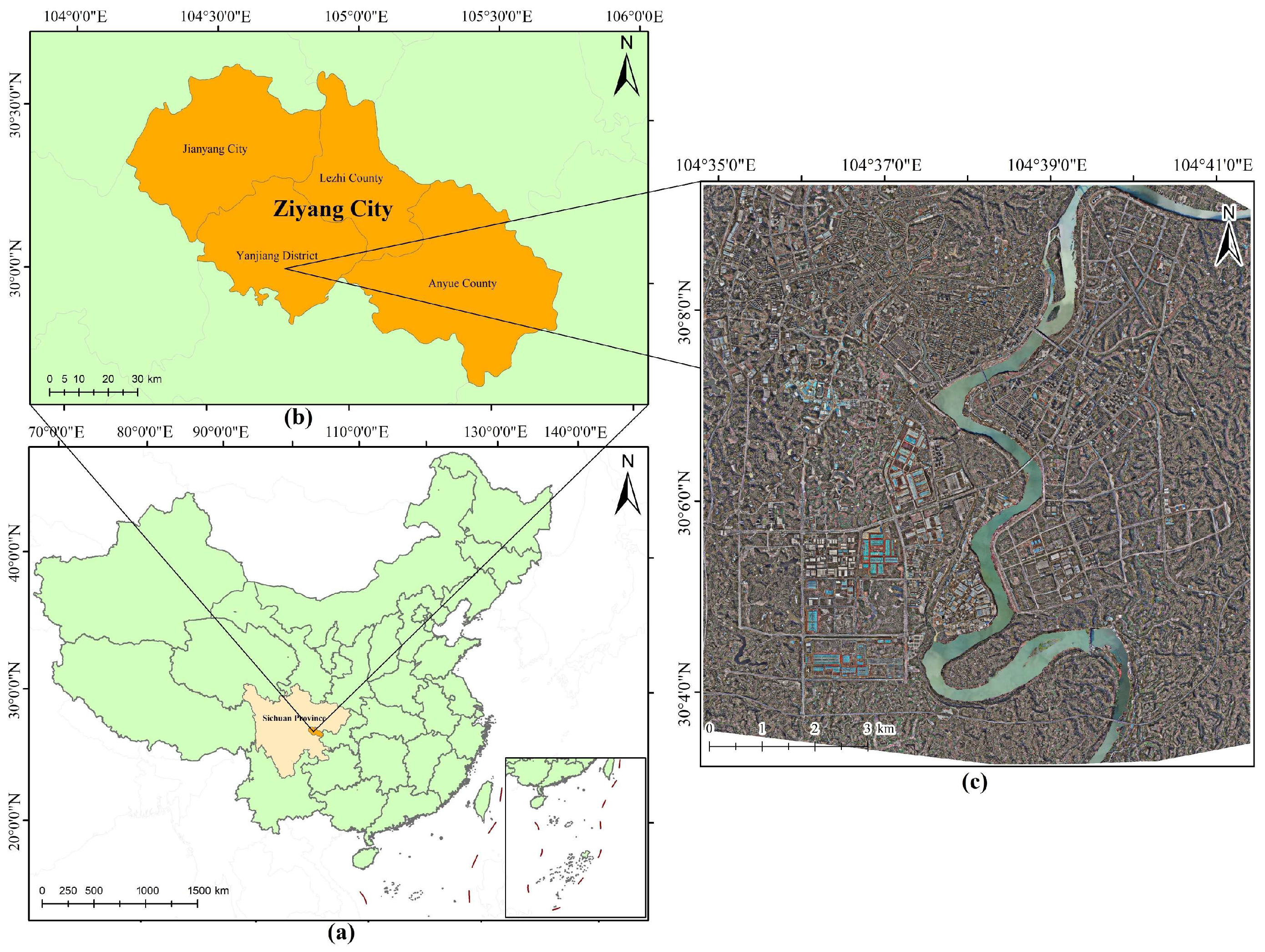
3.5.1. Sample Selection

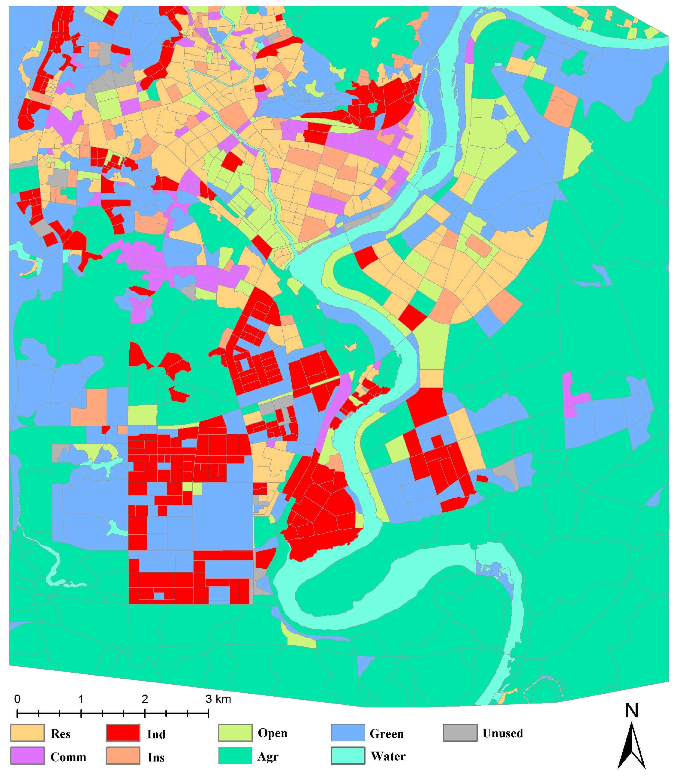
Our study area was characterized by a diverse range of functionalities, including residential housing, factories, hotels, shopping centers, and urban villages. Leveraging airborne images and high-precision Google Maps, we meticulously classified the study area into two distinct zones: built-up and non-built-up. This classification was based on a nuanced understanding of the social and economic characteristics of each city block, as well as the composition of the underlying surfaces. Within the built-up zones, there were identifiable segments such as residential areas, commercial districts, industrial sectors, institutional services, and open spaces. Conversely, the non-built-up zones encompass agricultural zones, green spaces, water, and unused zones. A detailed breakdown of these functional categories within the study area is presented in

Table 6. The categorization and description of UFZs in the study area.

UFZ	Abbreviation	Description
Built-up zone
Residential	Res	Residential areas, communities and affiliated facilities, urban villages, rural settlements, villas, traditional dwellings, etc.
Commercial	Comm	Financial services center, shopping service center, dining, hotels, entertainment facilities, retail center, etc.
Industrial	Ind	Heavy and light industrial zone, including refining, machinery, electronics manufacturing, food processing and pharmaceuticals, warehouses, etc.
Institutional	Ins	Scientific and educational cultural services, healthcare and hospital services, government institutions, and social organizations, etc.
Open space	Open	Construction sites, squares, stations, parking lots, etc.
Non-built-up zone
Agricultural	Agr	Vegetable plots, farmland, orchards, nurseries, and other agricultural cultivation areas.
Green space	Green	Wooded areas, grasslands, shrubbery, etc.
Water	Water	Rivers, lakes, reservoirs, ponds, etc.
Unused	Unused	Open land, bare ground, sandy areas, etc.

, providing a comprehensive overview of the diverse landscape and land cover patterns.

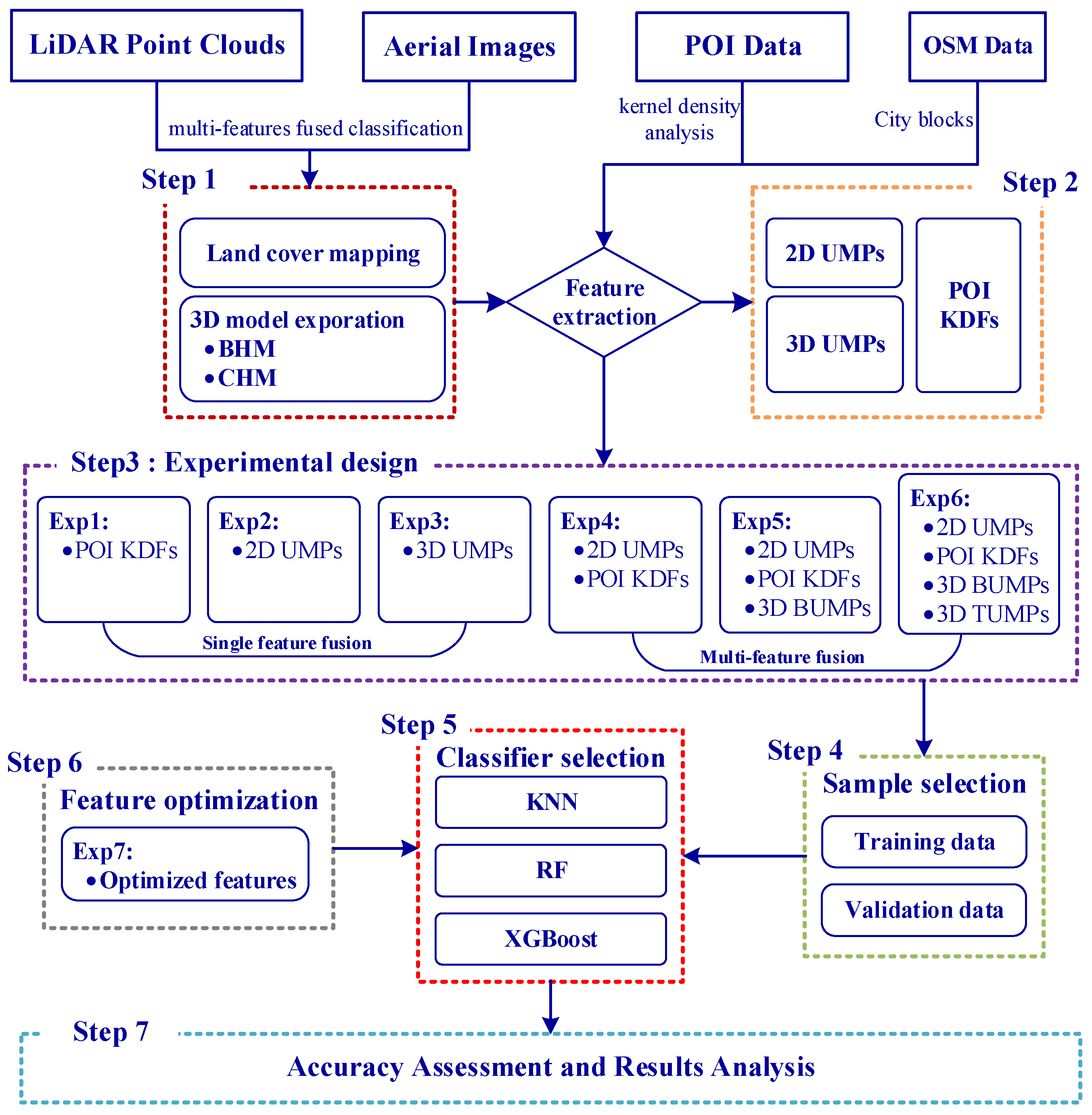
In machine learning algorithm, the process of selecting classification samples is a pivotal step that has a direct impact on the construction of models and the quality of the classification results. The sample dataset comprises both training data and validation data. The training data are employed to construct the learning model, whereas the validation data are utilized to assess the model’s capacity to discriminate new samples. The testing error on the validation data provides an approximation of the generalization error and is used to select the learning model. To avoid the impact of sample quantity and proportion imbalance on classifier training [45], we selected the sample dataset for each UFZ based on the spectral responses of objects on aerial images and existing geographic data. This process, combined with the delineation of city blocks and nine UFZs, resulted in the selection of sample datasets covering the entire study area and all categories. The number of samples for each UFZ was determined based on the proportion of each UFZ within the entire study area. The selection of the sample dataset involves several steps: Initially, we randomly generated sample dataset that spanned the entire study area without including any feature attribute information. Subsequently, we combined high-resolution Google Earth images with aerial images taken at similar times to label the sample dataset with specific categories. We then employed random sampling once again to divide the sample dataset into two sets: 70% training data and non-overlapping 30% validation data. Finally, we extracted the attribute information contained within the input features of each classification experiment and assigned it to the corresponding training and validation data. Following these steps, we prepared the sample dataset for Exp.1–6, with each sample data containing its associated input feature information. 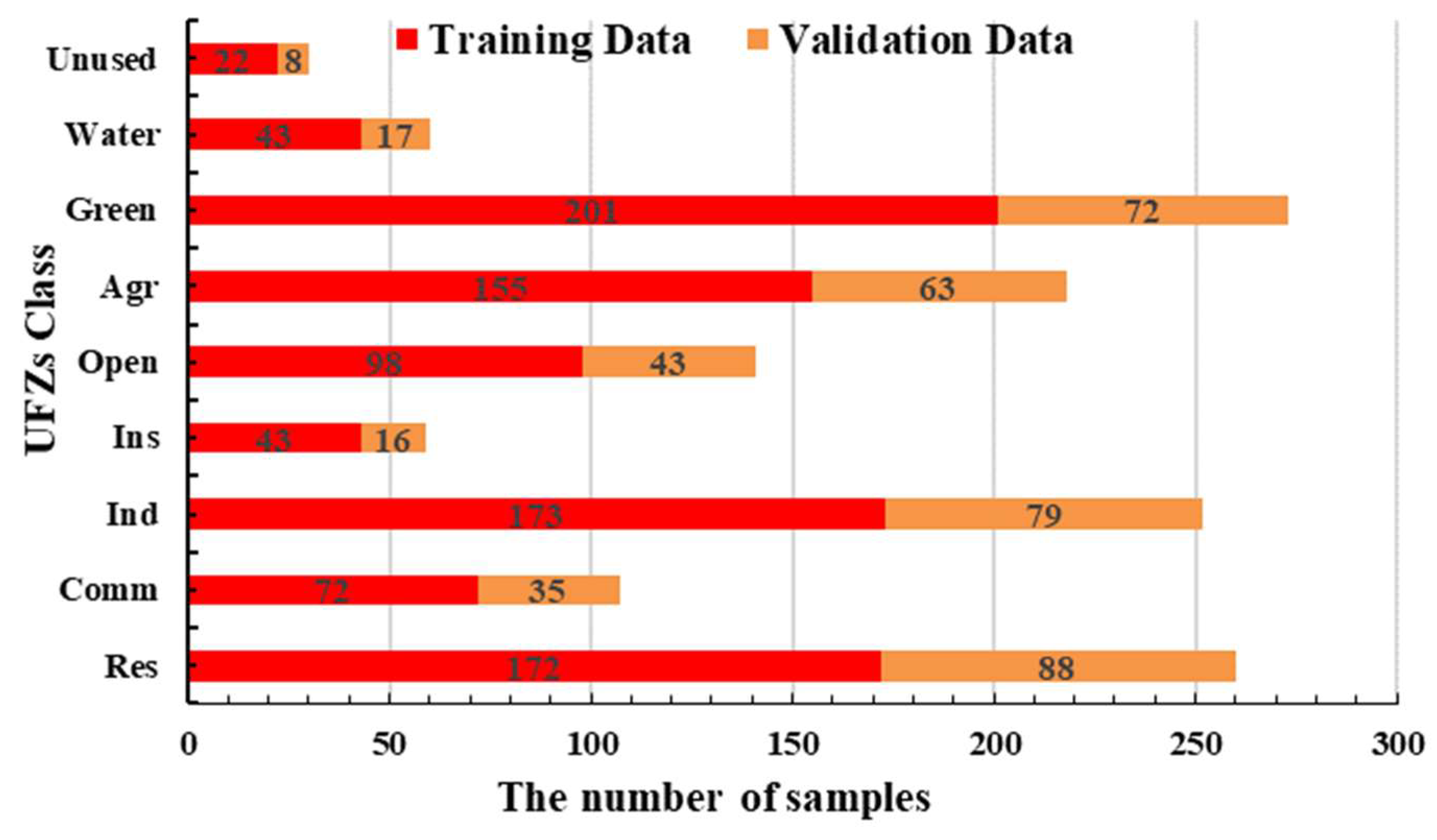Figure 6 displays the number of training and validation data samples for UFZ classification, indirectly indicating the approximate proportion of each UFZ within the study area.

3.5.2. Classifier Selection

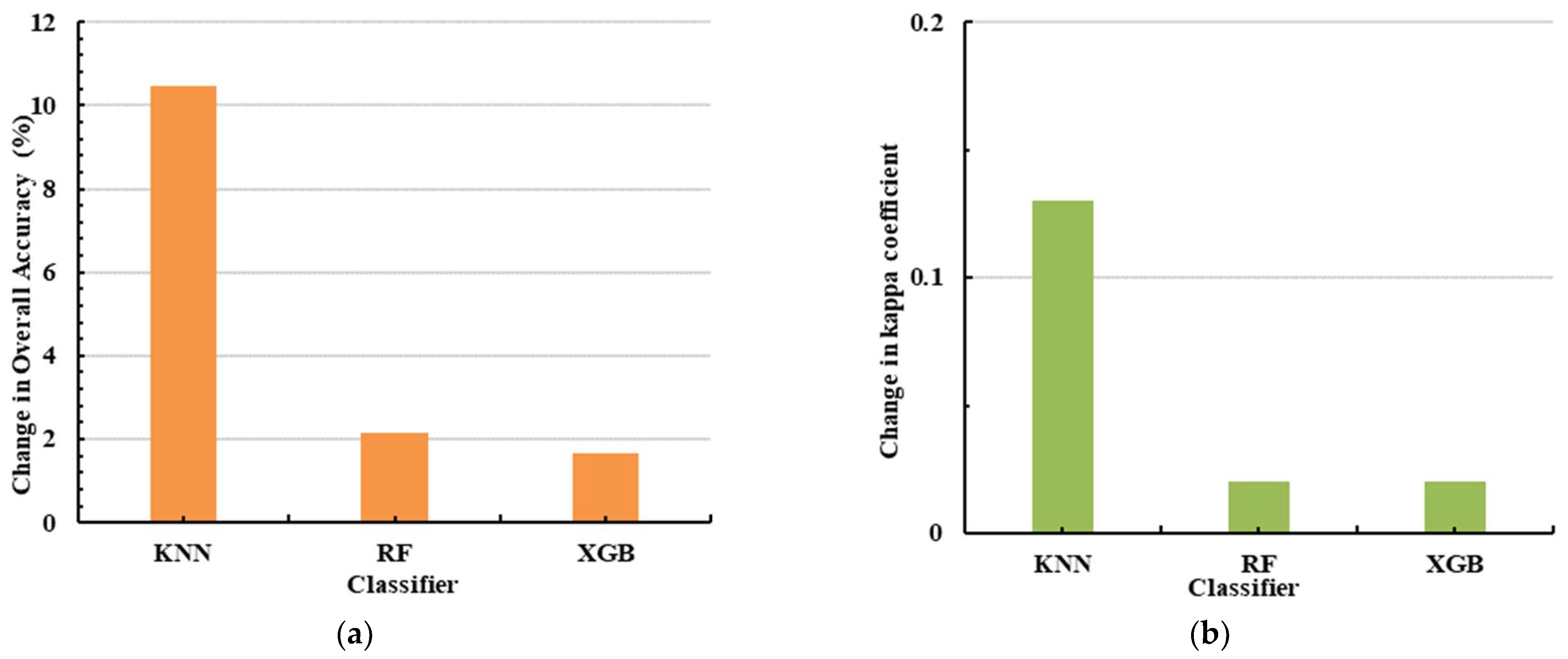
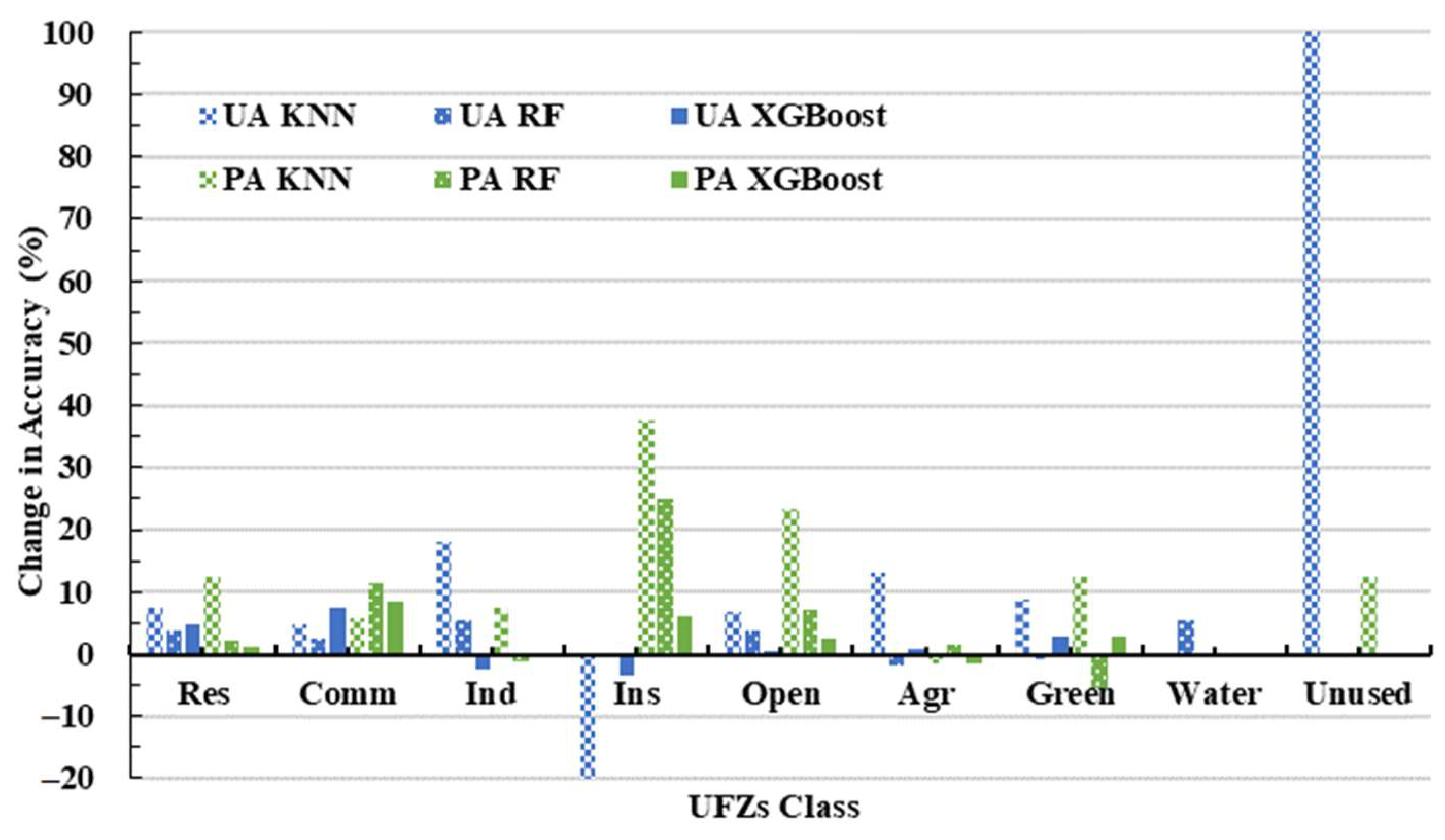
In this research, we carefully chose three machine learning algorithms for UFZ classification: KNN, RF, and XGBoost. Our objective was twofold. Firstly, we sought to evaluate the robustness and consistency of the classification experiments through a comprehensive analysis of the results obtained from these three classifiers. Secondly, we aimed to identify and select the classifier that delivered the highest classification performance to produce the UFZ classification map. The UFZ classification, leveraging these three classifiers, was executed within the Python 3.7 environment.

• KNN classifier

The KNN classifier is a widely used and powerful non-parametric machine learning algorithm in pattern recognition [46,47]. It stands out for its user-friendly nature, interpretability, robust predictive capabilities, resilience to outliers, and its unique ability to assess the uniformity of sample distribution based on the accuracy of the algorithm. Consequently, KNN is often integrated with other classifiers in the realm of remote sensing data classification research [25,48,49,50]. KNN is an instance-based lazy learning algorithm that does not require pre-training on a large set of samples to build a classifier. Instead, it stores all available instances and measures the similarity between samples based on distance calculations. The fundamental principle of KNN involves comparing the features of a new input sample, which lacks a classification label, to the features of every sample in the training data. It identifies the K-nearest (most similar) data and assigns the most frequently occurring class among these data as the classification label for the new input data [51]. The selection of the K value holds paramount importance in the classification process, given that both excessively large and small K values can potentially result in problems like over-regularization or an exaggerated emphasis on local distinctions [52]. In this study, we diligently conducted numerous trials to ascertain the optimal K value for achieving the highest classification accuracy by exploring values within a range of 0 < K < 50. To achieve this, we introduced an iterative algorithm that calculated the classification accuracy for each iteration. This was accomplished through cross-validation, using both training and validation data, and selecting the K value that corresponded to the highest validation data accuracy as the best choice.

• RF classifier

The RF classifier stands out as a non-parametric pattern recognition algorithm that operates as an ensemble classifier based on decision trees and bagging. Its classification predictions are reached by aggregating the results from a multitude of individual decision trees, essentially taking a collective vote from this ensemble of trees [53,54]. RF demonstrates remarkable capability in managing high-dimensional input samples without the need for dimensionality reduction. It operates without the requirement for any a priori assumptions regarding data distribution, ensuring efficiency even in experiments with limited sample sizes. Despite these attributes, it consistently delivers robust and reliable classification results. Furthermore, RF possesses the capability to assess the importance of input variables, adding to its versatility and utility in various classification research studies [53,55]. These characteristics render RF exceptionally effective in the realm of remote sensing data classification, spanning a wide array of data types including multispectral, hyperspectral, LiDAR, and multisource remote sensing data [56,57,58]. The fundamental principle of RF involves a series of steps: Starting with N samples and M feature variables, RF employs bootstrap sampling to randomly, and with replacement, draw 2N/3 independent samples from the original training data. These samples serve as the foundation for constructing individual decision trees, collectively forming the random forests. Within each tree, m feature variables (where m < M) are randomly and repeatedly selected to guide the branching process. The splitting of nodes within these trees is determined using the Gini criterion, a measure that identifies the variable offering the most optimal partitioning for the nodes [49]. The remaining data, known as out-of-bag (OOB) data, are used to evaluate the error rate of the random forest and to calculate the importance of each feature [57]. Through a series of iterations, OOB data are progressively used to eliminate less impactful features and select the most valuable ones. After OOB predicts results for all samples and compares them to the actual values, the OOB error rate is calculated. The classification of new sample data is determined by majority voting among the results from all constructed decision trees [59]. When confronted with a substantial number of input features, the heightened intercorrelation among variables can lead to a decline in both classification accuracy and computational efficiency. Consequently, the process of feature optimization becomes imperative, as it ensures the preservation of the most influential features that enhance classification accuracy while simultaneously eliminating the less pertinent ones. RF incorporates two significant parameters: the number of decision trees (ntree) and the number of randomly selected feature variables at each node split (mtry). Generally, ntree configuration is considered more critical since a higher number of trees increases model complexity but decreases efficiency [56,59]. For most RF applications, the recommended range for ntree values extends from 0 to 1000, with mtry often being set as the square root of the total number of input features [24,25,57]. In this study, we set mtry as the square root of the number of input features, while the ntree range was established from 0 to 1000 with 100-interval iterations to compute the model’s accuracy, thus determining the optimal ntree value.

• XGBoost classifier

XGBoost is a gradient boosting algorithm based on decision trees, falling within the realm of gradient boosting tree models. XGBoost undergoes iterative data processing across multiple rounds, generating a weak classifier at each iteration. The training of each classifier is rooted in the classification residuals acquired from the preceding iteration. These weak classifiers are distinguished by their simplicity, low variance, and high bias, exemplified by models like CART classifiers, and they are also amenable to linear classification. The training procedure consistently enhances classification accuracy by mitigating bias. The final classifier is crafted through an additive model, wherein each weak classifier obtained in every round of training is assigned weights and aggregated together [60]. XGBoost boasts several advantages, including regularization to reduce overfitting, parallel processing capabilities, customization of optimization goals and evaluation criteria, as well as handling sparse and missing values. Research has demonstrated that XGBoost provides high predictive accuracy and processing efficiency in remote sensing data analysis and classification applications [61,62,63]. XGBoost is frequently implemented alongside cross-validation and grid search, which are two crucial components in machine learning. The combination of cross-validation and grid search is the most commonly employed method for model optimization and parameter evaluation [64,65]. In machine learning, using the same dataset for both model training and estimation can result in inaccurate error estimation. To mitigate this issue, cross-validation methods are employed, offering more precise estimates of generalization error that closely reflect the actual performance of the model. In practical applications, k-fold cross-validation is commonly utilized, with k = 10 being a typical and empirically favored choice [66,67,68]. Grid search is an algorithm that leverages cross-validation to identify the optimal model parameters. It operates as an exhaustive search method, meticulously exploring candidate parameter choices to unearth the most favorable results. This algorithm systematically cycles through and evaluates every conceivable parameter combination, effectively automating the process of hyperparameter tuning [69]. In our research, we incorporated the k-fold cross-validation and grid search methods to enhance the efficiency of tuning multiple parameters while minimizing their interdependencies. The following parameters were optimized in our study to enhance model accuracy. Learning rate, representing the rate of learning, enhances model robustness by systematically reducing weights at each step. Our study meticulously examined its values, encompassing 0.0001, 0.001, 0.01, 0.1, 0.2, and 0.3, in order to pinpoint the optimal setting; n_estimators, denoting the quantity of decision trees, was fine-tuned within a range spanning from 1 to 1000, with iterations conducted at intervals of 1. The iterative process persisted until no further enhancements were evident in cross-validation error over 50 iterations; max_depth and min_child_weight are pivotal parameters exerting substantial influence on the ultimate results. We systematically adjusted their values, spanning from 1 to 10, with iterations occurring at 1-interval intervals; gamma, the controller of post-pruning tree behavior, designates the minimum loss reduction necessary for additional splits at a leaf node. Higher values reflect a more conservative approach. Our study meticulously examined a range of values, spanning from 0 to 0.5, with iterations conducted at 0.1 intervals; subsample, a parameter governing the random selection of training data for each tree, plays a key role in the algorithm’s balance between conservatism and susceptibility to overfitting. Our study encompassed values ranging from 0.6 to 1, with iterations occurring at 0.1 intervals to identify the most suitable setting; colsample_bytree, responsible for column sampling during tree construction, dictates the ratio of columns randomly chosen for each tree, and we explored a range of values from 0.6 to 1, conducting iterations at 0.1 intervals; reg_alpha, serving as the L1 regularization term for weights, bolsters the algorithm’s computational efficiency in high-dimensional training samples. Our study delved into values ranging from 10⁻⁵, 10⁻², 0.1, and 1 to 100 for this parameter.

3.5.3. Feature Optimization

When dealing with a substantial number of input features, the increased intercorrelation among variables can lead to a decline in classification accuracy and computational efficiency. Therefore, it is imperative to optimize these numerous input features, preserving those that significantly contribute to the model’s classification accuracy and eliminating the less influential ones, to achieve optimal precision. In the realm of classification research, RF algorithm is frequently employed to assess variable importance. There are two primary methods for evaluating variable importance: Mean Decrease Impurity (MDI), often referred to as GINI importance, evaluates the value of a node by quantifying the reduction in impurity during its division. Mean Decrease in Accuracy (MDA), based on OOB error, examines the effect on classification accuracy when specific feature values are randomly interchanged within OOB data. Notably, MDA tends to yield results with greater accuracy than MDI [53,54].

The MDA of $X\left(j\right)$ is calculated by averaging the difference in OOB error estimation before and after permutation across all trees [70]. A higher MDA value indicates greater variable importance. The formula for calculating the importance of feature $j$ (the $j\mathrm{th}$ dimension of the sample) is as follows:

$${\mathrm{MDA}}_{\mathrm{c}}\left(j\right)=\frac{1}{T}{{\displaystyle \sum }}_t^T\left[\frac{1}{\left|D_t\right|}\left({{\displaystyle \sum }}_{x_i-D_t}I\left(P\left(X_i=y_i\right)\right)-{{\displaystyle \sum }}_{x_i^j-D_i^j}I\left(P\left(X_i^j=y_i\right)\right)\right)\right],$$

(2)

where $T$ represents the number of random trees $\left(X_i, y_i\right)$ that represent the sample, with $y$ representing the class label. $X_i^j$ denotes the sample resulting from the random exchange of the $j$-th dimension (feature) of $X_i$; $D_t$ is the OOB sample dataset for random tree $t$ and $D_t^j$ represents the sample dataset formed after exchanging the $j$-th dimension; $P\left(X_i\right)$ represents the prediction (class) for sample $X_i$; $I\left(P\left(X_i=y_i\right)\right)$ is the indicator function, returning 1 if the prediction matches the true class label, and 0 otherwise.

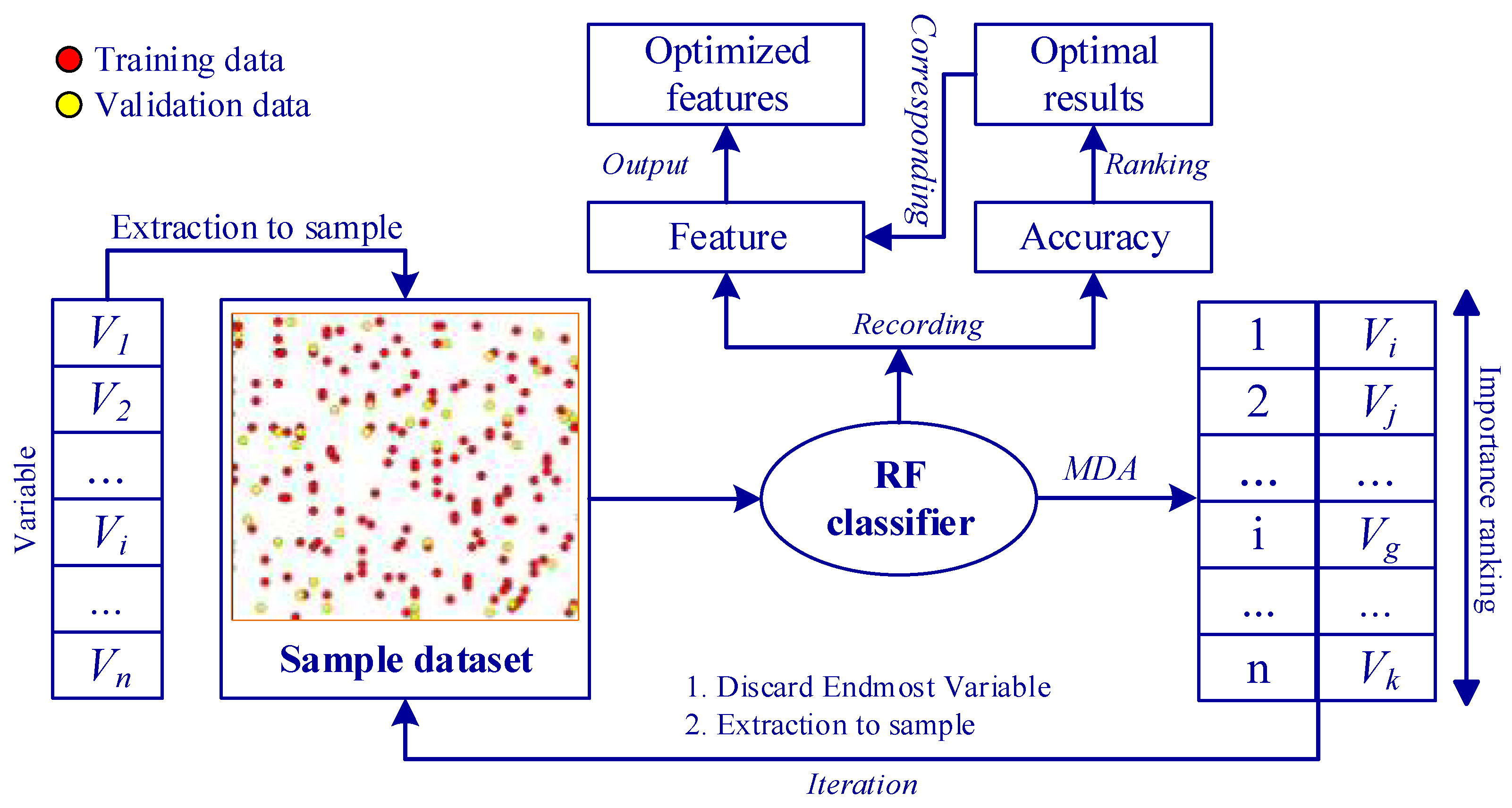
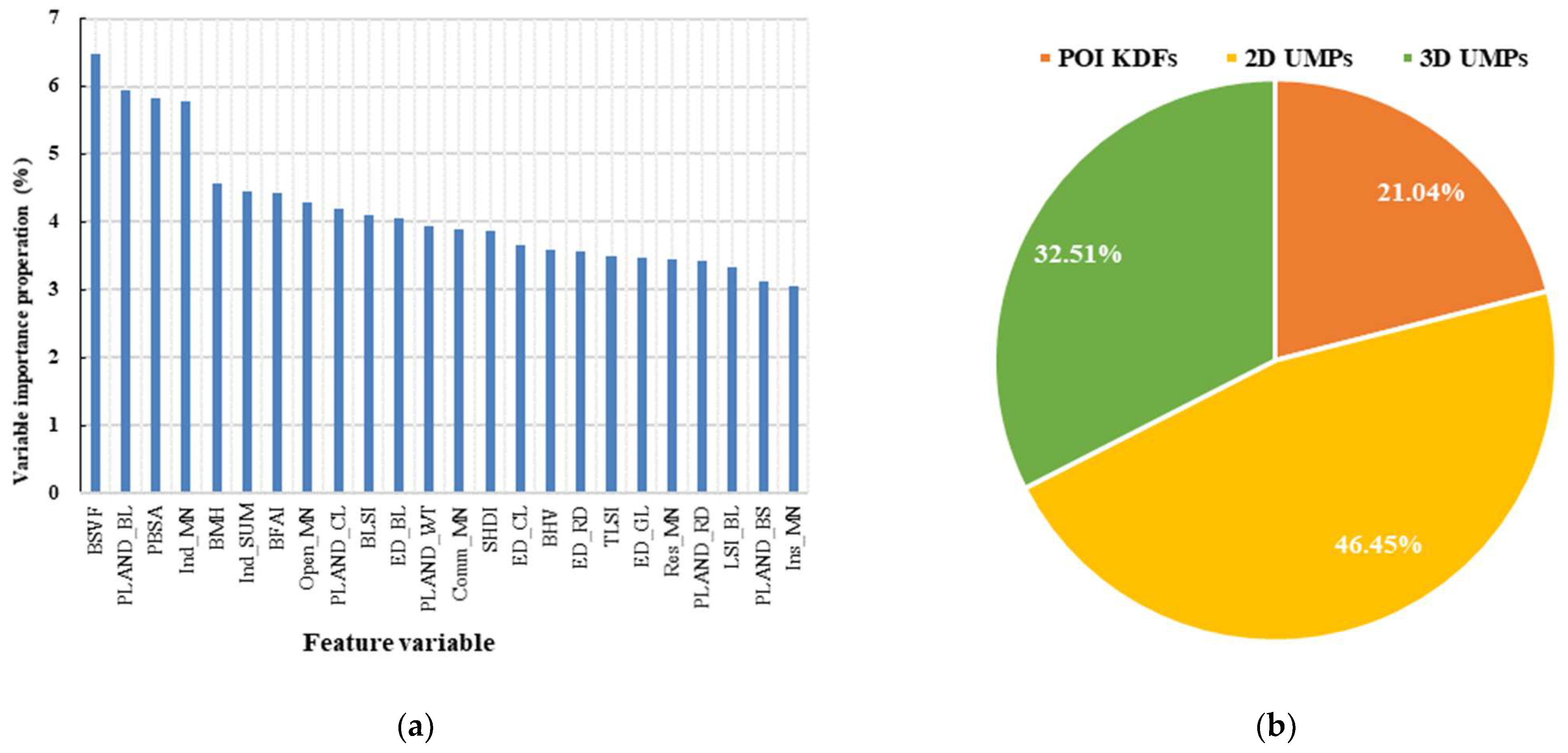
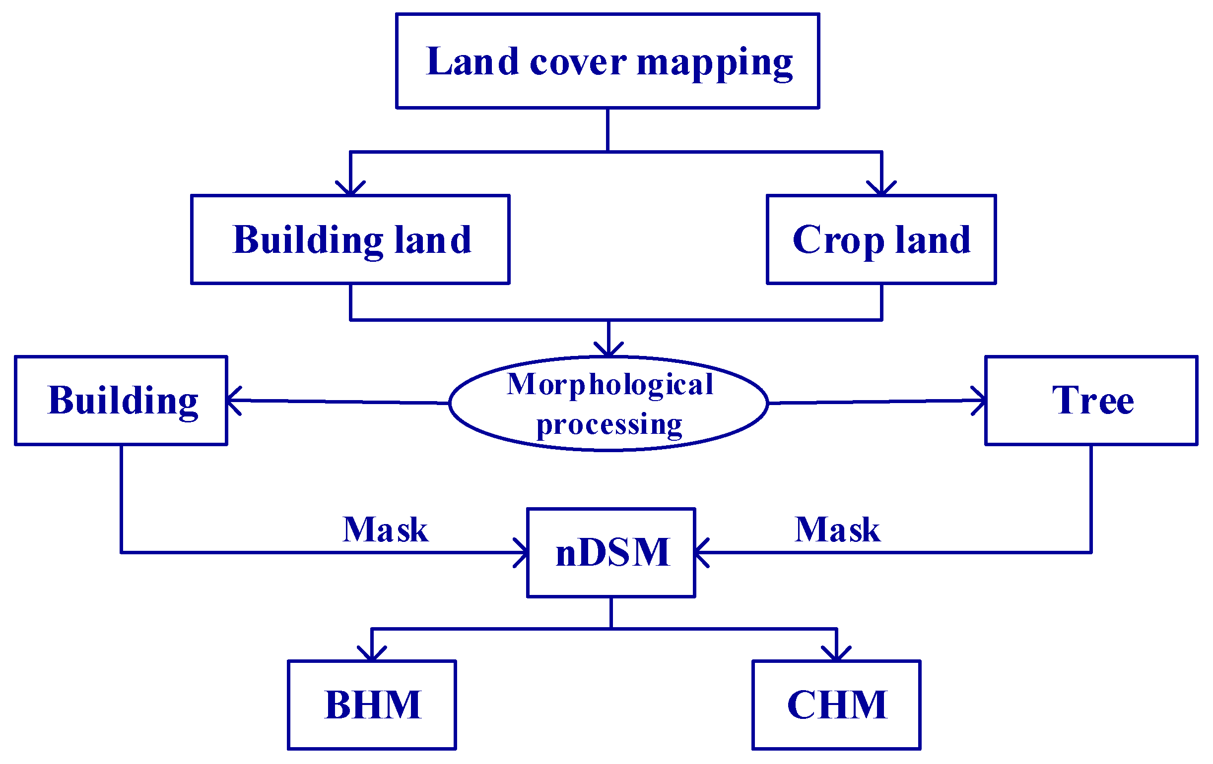
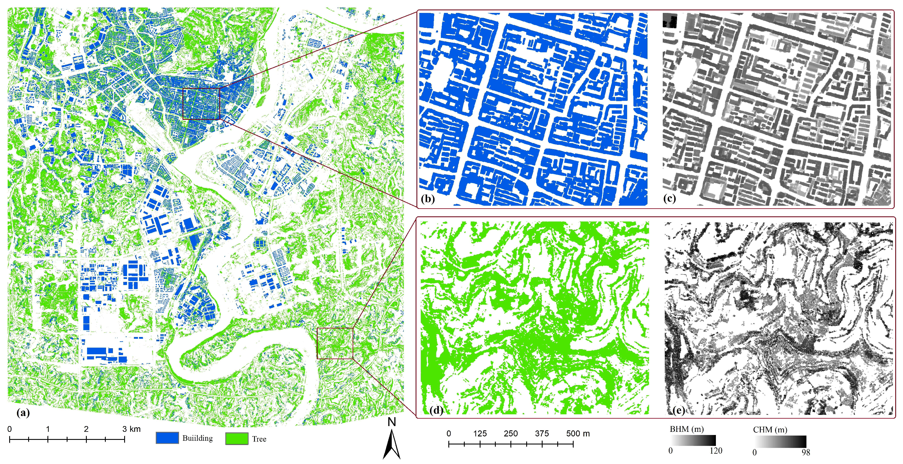
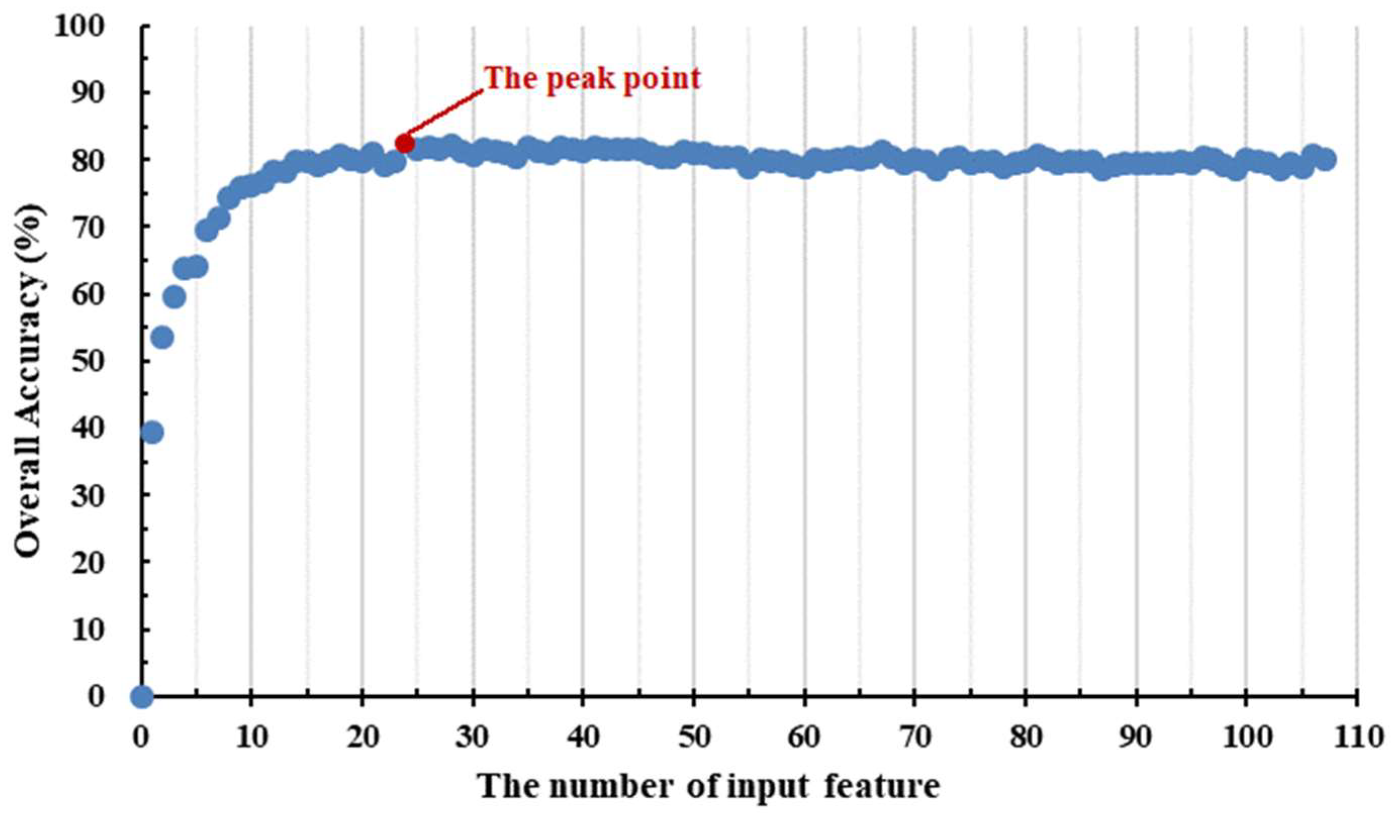
In our research, we employed the MDA method to evaluate variable importance and implement feature optimization to pinpoint the optimal features for a refined classification experiment (Exp.7). Figure 7 illustrates the workflow of feature optimization via the RF classifier, particularly when managing high-dimensional input features. To begin with, we extracted the attribute values of all features (variables) to their corresponding samples, denoted as $V=\left(V_1,V_2,V_3\cdots V_n\right)$. The sample dataset was then trained using the RF classifier. Subsequently, variables were ranked based on their MDA values, and the least important ones were identified. These least important variables were then excluded from the input variables, and the attribute values of the remaining variable amalgamation were reintroduced into the sample dataset. Another round of training was executed with the RF classifier. This process was iterated until the number of input variables reached zero. Throughout the iterations, we recorded the variables involved in RF training and the resulting classification accuracy. Finally, we ranked all the recorded accuracies, found the best classification result and its corresponding variables, and then output the optimal variable combination for Exp.7. In this paper, we introduced the variable importance proportion (VIP), which represents the feature contribution to classification by indicating the proportion of each variable’s importance relative to the overall variable importance.

3.6. Accuracy Assessment

Accuracy assessment is a crucial aspect of UFZ classification research. The quality of classification accuracy acts as a key indicator for both model optimization and the design of classification experiments. Moreover, understanding and analyzing the root causes and distribution trends of classification errors are of paramount importance in improving classification results and further refining classification methods.

Confusion Matrix (CM) stands as a standard format for precision evaluation. Its assessment primarily hinges on comparing the degree of confusion between classification outcomes and ground truth values [71]. This method has been widely adopted in remote sensing data classification studies [11,48]. Leveraging CM enables us to grasp the total sample count for each UFZ category and the numbers of misclassified and omitted samples, rendering our classification outcomes more intuitively presentable. CM is depicted in an $n\times n$ matrix format, summarizing the records in the dataset based on actual category judgment against predicted category judgment from the classification model. Here, the matrix rows represent the reference category values of samples, while the columns indicate predicted sample category values [70]. Typical evaluation metrics from CM encompass OA, UA, PA, and the kappa coefficient. OA and the kappa coefficient reflect the comprehensive classification precision of the entire image, while UA and PA illuminate the classification precision of individual categories. Moreover, based on research [72], the kappa coefficient is interpreted as follows: 0.8–1.0 (almost perfect); 0.6–0.8 (substantial); 0.4–0.6 (moderate); 0.2–0.4 (fair); 0–0.2 (slight). These interpretations also provide a valuable reference for us to evaluate the quality of our classification results.

4. Results

4.1. Classification Results of Multi-Feature Fusion

Table 7. The classification results from six multi-feature fusion experiments are based on KNN, RF, and XGBoost, encompassing OA and kappa coefficient.

Exp.#	OA (%)			Kappa Coefficient
	KNN	RF	XGBoost	KNN	RF	XGBoost
Exp.1	55.58	56.06	58.43	0.47	0.47	0.5
Exp.2	60.57	66.27	67.46	0.53	0.59	0.61
Exp.3	61.52	67.7	67.46	0.54	0.61	0.61
Exp.4	68.41	79.1	82.66	0.62	0.75	0.79
Exp.5	68.88	80.76	83.14	0.63	0.77	0.8
Exp.6	69.83	80.56	84.56	0.64	0.77	0.82
Exp.1	55.58	56.06	58.43	0.47	0.47	0.5

provides a comprehensive view of the classification results obtained from six multi-feature fusion experiments employing KNN, RF, and XGBoost. Notably, Exp.6, whose combination features are related to POI KDFs, 2D UMPs, 3D BUMPs, and 3D TUMPs, demonstrated the highest classification accuracy among the six experiments (OA = 84.56%, kappa coefficient = 0.82). Additionally, XGBoost performed best among the three classifiers. After a thorough analysis and comparison of the classification results from the three single source data experiments (Exp.1–3), certain trends emerged. In both KNN and RF classifiers, Exp.3, which incorporated 3D UMPs as input features, displayed a notably more substantial enhancement in classification accuracy when contrasted with Exp.2, where 2D UMPs were employed as input features. However, within the framework of XGBoost classifier, the results for Exp.2 and Exp.3 remained consistent, resulting in an OA of 67.46% and a kappa coefficient of 0.61. In contrast, Exp.1, which relied exclusively on POI KDFs as input features, demonstrated the poorest classification performance. Upon thoroughly observing and analyzing the classification results generated by the fusion of multisource data (Exp.4–6), it became apparent that the inclusion of new features led to a significant enhancement in classification accuracy. Particularly, in Exp.4, where 2D UMPs were combined with POI KDFs, a substantial improvement in accuracy was evident when compared to Exp.1. This enhancement was particularly pronounced in the OA, which increased by 12.83% to 24.23%, and the kappa coefficient, which rose by 0.15 to 0.29. The addition of 3D UMPs further enhanced classification performance. Specifically, the inclusion of 3D BUMPs in Exp.5 led to an increase in OA ranging from 0.47% to 1.66% and an increment in the kappa coefficient by 0.01 to 0.02 when compared to Exp.4. However, as the number of features increased, the magnitude of accuracy improvement significantly decreased. In the case of Exp.6, where 3D TUMPs were introduced, resulting in a total of 107 input features, the impact on classification accuracy varied among the classifiers. Notably, XGBoost demonstrated a noteworthy increase in OA by 1.42%, whereas the OA in the KNN classifier rose by only 0.95% and remained below 70%. Conversely, RF experienced a slight 0.2% decrease in OA compared to Exp.5. This observation suggested that the heightened correlation and redundancy between features constrained the enhancement in classification accuracy and, in some instances, even led to a decrease. When we scrutinized the performance of the classifiers, it became evident that XGBoost consistently demonstrated exceptional stability and maintained a high classification accuracy, even as the number of input features increased to 107. This clearly indicated that XGBoost excelled in handling high-dimensional input features. In contrast, while RF achieved a classification accuracy exceeding 80%, its accuracy exhibited a tendency to decrease as the number of input features increased. On the other hand, KNN displayed poor stability when processing high-dimensional input features, with its classification results significantly falling short of the performance achieved by RF and XGBoost.

Table 8. The statistics of UA and PA in six multi-feature fusion experiments using KNN, RF, and XGBoost.

UFZ	UA (%)			PA (%)
	KNN	RF	XGBoost	KNN	RF	XGBoost
Exp.1
Res	60.78	59.0	61.62	70.45	67.05	69.32
Comm	66.67	60.0	62.07	51.43	51.43	51.43
Ind	63.73	68.75	69.79	82.28	83.54	84.81
Ins	66.67	46.15	60.0	37.5	37.5	37.5
Open	38.46	42.11	42.86	34.88	37.21	41.86
Agr	51.55	58.21	62.32	79.37	61.9	68.25
Green	42.86	41.33	45.07	25.0	43.06	44.44
Water	0	100.0	25.0	0	5.88	5.88
Unused	0	0	0	0	0	0
Exp.2
Res	61.74	66.67	69.61	80.68	86.36	80.68
Comm	44.44	36.36	42.11	34.29	11.43	22.86
Ind	58.44	61.54	60.0	56.96	70.89	64.56
Ins	0	0	33.33	0	0	18.75
Open	60.61	67.74	69.44	46.51	48.84	58.14
Agr	63.41	76.92	76.47	82.54	79.37	82.54
Green	62.3	61.11	67.9	52.78	76.39	76.39
Water	94.44	100.0	100.0	100.0	100.0	100.0
Unused	0	0	50.0	0	0	25.0
Exp.3
Res	67.89	78.79	80.61	84.09	88.64	89.77
Comm	27.27	66.67	50.0	8.57	28.57	34.29
Ind	62.89	70.71	73.96	77.22	88.61	89.87
Ins	0	25.0	20.0	0	6.25	6.25
Open	68.42	53.33	55.00	30.23	37.21	25.58
Agr	65.75	67.21	73.77	76.19	65.08	71.43
Green	53.19	59.78	56.67	69.44	76.39	70.83
Water	55.56	73.68	56.0	58.82	82.35	82.35
Unused	0	0	0	0	0	0
Exp.4
Res	70.54	80.58	87.78	89.77	94.32	89.77
Comm	72.73	82.61	83.33	45.71	54.29	71.43
Ind	74.39	84.52	90.0	77.22	89.87	91.14
Ins	75.0	85.71	66.67	18.75	37.5	62.5
Open	62.96	83.33	80.49	39.53	58.14	76.74
Agr	60.67	79.71	80.6	85.71	87.3	85.71
Green	60.29	64.77	73.08	56.94	79.17	79.17
Water	100.0	100.0	100.0	100.0	100.0	100.0
Unused	0	0	33.33	0	0	12.5
Exp.5
Res	73.33	84.0	85.71	87.5	95.45	95.45
Comm	71.43	76.67	84.62	42.86	65.71	62.86
Ind	71.43	89.02	92.41	82.28	92.41	92.41
Ins	66.67	100.0	80.0	12.5	31.25	75.0
Open	72.73	80.56	85.0	37.21	67.44	79.07
Agr	62.96	78.46	77.61	80.95	80.95	82.54
Green	60.26	67.06	71.43	65.28	79.17	76.39
Water	94.44	100.0	100.0	100.0	100.0	100.0
Unused	0	100.0	50.0	0.0	12.5	12.5
Exp.6
Res	75.25	83.17	86.32	86.36	95.45	93.18
Comm	79.17	80.77	82.14	54.29	60.0	65.71
Ind	72.04	87.06	94.81	84.81	93.67	92.41
Ins	100.0	80.0	80.0	12.5	25.0	75.0
Open	69.57	77.78	79.07	37.21	65.12	79.07
Agr	61.8	79.41	81.43	87.3	85.71	90.48
Green	58.33	69.51	76.0	58.33	79.17	79.17
Water	100.0	94.44	100.0	100.0	100.0	100.0
Unused	0.0	0.0	100.0	0.0	0.0	12.5

provides a detailed overview of the results for UA and PA obtained from the six multi-feature fusion experiments. A closer examination of the accuracy within the three single data source experiments (Exp.1–3) revealed that in Exp.1, the POI KDFs exhibited strong performance in classifying residential, commercial, industrial, and agricultural zones, achieving UA and PA values exceeding 50%. However, its performance was comparatively weaker in classifying water and unused zones. This limitation could be attributed to the concentration of POI KDFs in built-up zones, which restricted their ability to effectively differentiate UFZs in non-built-up zones. Institutional zones and open spaces, being characterized by mixed distributions with residential, commercial, and industrial zones, presented additional challenges for accurate classification. In the classification of residential zones, industrial zones, agricultural zones, and water, the 2D UMPs displayed strong performance, with both UA and PA exceeding 50%. However, they were less effective when it came to classifying institutional and unused zones. This was primarily because 2D UMPs primarily described the landscape composition and spatial distribution based on land covers within city blocks. In some UFZs like residential, commercial, and industrial zones, where detailed 3D information and functional descriptions were lacking, distinguishing them became a more challenging task. The 3D UMPs proved to be effective in classifying residential, industrial, and agricultural zones, as these zones exhibited distinct 3D characteristics. However, their performance was less effective when it came to classifying institutional and unused zones.

After closely observing the classification results obtained from the fusion of multisource data in Exp.4–6, it was evident that the fused classification accuracy had notably improved when compared to using a single data source. Therefore, we conducted a comprehensive analysis and comparison of the classification accuracy for nine UFZs (Table 8) and examined the accuracy variations between different experiments, as visually represented in Figure 8.

Figure 8a illustrates the changes in accuracy at the class level in Exp.4 compared to Exp.1, i.e., the differences in accuracy for nine UFZs between Exp.4 and the corresponding values in Exp.1. It is evident that the fusion of POI KDFs and 2D UMPs significantly enhanced the accuracy of UFZs. This enhancement was most notable in water, with UA and PA showing changes within the range of 75–100% (except for the UA in the RF classifier, which remained unchanged). Residential zones, open spaces, agricultural zones, and green spaces also experienced substantial increases in accuracy, with improvements exceeding 20%. Similarly, commercial, industrial, and institutional zones showed corresponding increases in classification accuracy, with both XGBoost and RF consistently improving. In contrast, KNN exhibited a negative change in PA for these three types of UFZs. Only XGBoost demonstrated a positive increase in accuracy for unused zones, with growth rates ranging from 12.5% to 33.3%.

Figure 8b depicts the changes in accuracy at the class level in Exp.4 compared to Exp.2, showing the impact of introducing POI KDFs on 2D UMPs. It is evident that this combination effectively enhanced the classification accuracy of UFZs. This effect was particularly pronounced within built-up zones, with notable improvements in the classification accuracy of residential, commercial, industrial, and institutional zones. Some metrics even showed an improvement of over 40% in commercial and industrial zones. In contrast, the classification accuracy of open spaces in built-up zones showed a lower increase, but some metrics still displayed improvements of over 10%. This was because open spaces have fewer POI distribution points, and these points were often mixed with those of other UFZs, making the KDFs less distinct. The addition of POI KDFs had a smaller impact on the classification accuracy of UFZs in non-built-up zones. This was because POI KDFs were primarily distributed in urban central areas, and the characteristics of non-built-up zones such as agricultural zones and green spaces were less pronounced or almost non-existent. In summary, we found that the fusion of POI KDFs with 2D UMPs effectively enhanced the classification accuracy of UFZs. POI KDFs contributed significantly to improving the classification accuracy in built-up zones, while 2D UMPs played a substantial role in enhancing the accuracy of all the UFZs.

Figure 8c demonstrates the changes in class-level accuracy in Exp.5 compared to Exp.4. It is evident that the integration of 3D BUMPs with POI KDFs and 2D UMPs had a significant positive impact on the accuracy of unused zones, with improvements ranging from 12.5% to 100%. However, the improvements in the other eight UFZs were smaller, and some metrics even showed negative changes. A similar trend was observed in Figure 8d when 3D TUMPs were introduced in Exp.6. Here, we observed inconsistent improvements in the classification accuracy of UFZs, with minimal enhancements. This indicates that the increased correlation between input features and the varying classification abilities of different classifiers for high-dimensional input features led to inconsistent growth in some metrics. Moreover, an analysis of the OA confirmed this observation. XGBoost continued to enhance classification accuracy through model optimization, while RF exhibited negative growth, and KNN displayed a lower classification accuracy. Consequently, it was necessary to further compare and analyze the classification results of experiments through feature optimization.

4.2. Performances of Feature Optimization

In this study, we carried out comprehensive feature optimization to refine all 107 input features. We based our optimization on the observed trend of OA concerning the number of input features. This approach allowed us to identify the optimal number of input features that led to the highest OA and, consequently, discover the corresponding features associated with this peak performance. Figure 9 provides a visual representation of the relationship between OA and the number of input features. The graph revealed a distinct pattern in which OA experiences significant growth as the number of input features ranges from 0 to 10. As the number of input features increased from 10 to 24, the rate of OA growth became notably slower. When the input feature count extended from 24 to 107, OA initially showed a gradual decline before stabilizing. As a result of this analysis, we were able to pinpoint that the maximum OA was attained when the number of input features was 24. These 24 features were then carefully selected for the further verification of their impact on classification performance using three classifiers.

Table 9. Classification results based on the KNN, RF, and XGBoost after feature optimization, including OA and kappa coefficients.

Exp.#	OA (%)			Kappa Coefficient
	KNN	RF	XGBoost	KNN	RF	XGBoost
Exp.7	80.29	82.66	86.22	0.77	0.79	0.84

presents the results for the OA and kappa coefficients derived from the optimized feature fusion for the three classifiers. Clearly, XGBoost consistently outperformed the others by achieving the highest classification accuracy, boasting an OA of 86.22% along with an impressive kappa coefficient of 0.84. On the other hand, RF secured an OA of 82.66% with a kappa coefficient of 0.79. Although KNN fell short of RF in terms of performance, it maintained a commendable classification accuracy, posting an OA of 80.29% and a kappa coefficient of 0.77.

By comparing the changes in accuracy before and after feature optimization, we obtained the accuracy change chart shown in Figure 10 by subtracting the corresponding OA and kappa coefficients of Exp.7 from Exp.6. We observed that KNN experienced the most significant increase in accuracy, with its OA improving by 10.46% and its kappa coefficient increasing by 0.13. RF also showed notable improvement, with an OA increase of 2.14% and a kappa coefficient increase of 0.02. XGBoost exhibited a 1.66% increase in OA and a 0.02 rise in the kappa coefficient when compared to its performance with the fusion of all the input features used in Exp.6. In summary, after feature optimization, three classifiers demonstrated varying degrees of improved classification accuracy. Consequently, we considered feature optimization to be a necessary step in the experimental design, as the optimized features significantly contributed to the enhancement in both classification accuracy and efficiency across the three classifiers. In summary, the results after feature optimization indicate that all three classifiers demonstrated varying degrees of enhanced classification accuracy. This underscores the significance of feature optimization in our experimental design, as it evidently played a pivotal role in augmenting both the accuracy and efficiency of these three classifiers.

Table 10. The statistics of UA and PA for optimized feature fusion experiment based on the KNN, RF, and XGBoost.

UFZ	UA (%)			PA (%)
	KNN	RF	XGBoost	KNN	RF	XGBoost
Res	82.86	86.87	91.21	98.86	97.73	93.18
Comm	84.0	83.33	89.66	60.0	71.43	65.71
Ind	90.12	92.41	92.41	92.41	92.41	92.41
Ins	80.0	80.0	76.47	50.0	50.0	75.0
Open	76.47	81.58	79.55	60.47	72.09	81.40
Agr	75.0	77.46	82.35	85.71	87.30	84.13
Green	67.11	68.83	78.67	70.83	73.61	81.94
Water	100.0	100.0	100	100.0	100.0	100.0
Unused	100.0	0	100	12.5	0	12.5

presents the accuracy statistics for three classifiers at the class level after feature optimization in Exp.7. We observed that the UA and PA for residential zones, industrial zones, agricultural zones, and water all exceed 75%, with water achieving a remarkable accuracy rate of 100%. Commercial zones, open spaces, and green spaces exhibited both UA values and PA values surpassing 60%, while industrial zones maintained UA values and PA values above 50%. However, the classification accuracy for unused zones was notably poorer. This was due to the frequent coexistence of unused zones with other UFZs, which made it challenging to discern distinctive features. Commercial zones, open spaces, and green spaces exhibited both UA and PA values exceeding 60%, while industrial zones maintained UA and PA values above 50%. However, the classification accuracy for unused zones was notably lower. This could be attributed to the frequent coexistence of unused zones with other UFZs, which made it challenging to discern distinctive features.

Figure 11 provides a detailed insight into the changes in class-level accuracy observed in Exp.7 in comparison to Exp.6. Notably, Exp.7, benefiting from its optimized feature fusion, outperformed Exp.6, which utilized all input features. This led to an enhancement in accuracy across a diverse range of UFZs. All three classifiers displayed positive trends in accuracy for residential zones, commercial zones, open spaces, water, and unused zones. Although some minor negative trends were observed for industrial zones, institutional zones, agricultural zones, and green spaces, these declines were relatively modest in magnitude. Consequently, following the optimization process, there was a noticeable overall improvement in accuracy for each UFZ, coupled with a significant reduction in the disparities between the different classifiers. These outcomes underscore the benefits of feature optimization in bolstering both classifier stability and UFZ accuracy.

Ultimately, guided by the remarkable results obtained from the XGBoost classifier in the optimized experiments (Exp.7), we produced the UFZ classification map for the study area, which is visually represented in Figure 12.

4.3. Variable Importance Analysis

Figure 13a presents a visual representation of the variable importance ranking for the 24 optimized features. Notably, within the 3D UMPs, the BSVF emerged as the primary contributor to UFZ classification. Following closely, within the 2D UMPs, the PLAND of Building (PLAND_BL) played a pivotal role. Among the 3D UMPs, PBSA and BMH secured the third and fifth positions, respectively. Furthermore, within the POI KDFs, the Mean KDFs of Industrial (Ind_MN) claimed the fourth spot. It was essential to highlight that, among the top five features with the most substantial contributions to the classification, the 3D UMPs exhibited the highest influence, followed by the 2D UMPs, with the POI KDFs trailing slightly behind. Upon scrutinizing the distribution of the 24 features, it is evident that they encompassed four POI KDFs, twelve 2D UMPs, and seven 3D UMPs. We have meticulously summarized the VIP for these three feature types separately, as depicted in Figure 13b. It is notable that 2D UMPs hold a significant VIP share of 46.46%, surpassing the 32.51% VIP value associated with 3D UMPs. In contrast, POI KDFs contributed a modest 21.04% to the VIP for the classification results. This emphasized that, both in terms of quantity and VIP value, 2D UMPs took precedence over 3D UMPs, while POI KDFs exhibited a comparatively lower impact. In conclusion, within the multisource data fusion process for UFZ classification, 2D and 3D UMPs assumed a central position, with 3D UMPs demonstrating substantial influence. Conversely, while the contribution of POI KDFs was relatively modest, their capacity to reflect spatial distribution patterns of human activities, economic dynamics, and societal attributes remained of paramount significance.

5. Discussion

The accurate classification of UFZs provides a critical reference for urban planning and management. Previous research on UFZ classification primarily focused on megacities such as Beijing, Wuhan, New York, and Munich [5,13,15,18,19]. However, for medium-sized cities, particularly those in rapid development, a comprehensive understanding of UFZ classification becomes increasingly crucial. This study presents an innovative classification scheme designed specifically for medium-sized cities. By grasping the distribution characteristics and current situation of UFZs, effective and systematic urban planning can be achieved, promoting efficient resource allocation.

Achieving a more precise classification of UFZs necessitates a consideration not only of the landscape distinctions between these zones but also the incorporation of insights into socio-economic activities. Therefore, the integration of diverse remote sensing and social data stands as a prevailing trend in the research on UFZ classification [15,18,19]. In our study, we utilized ALS systems that simultaneously acquired high-precision LiDAR point clouds and aerial images, extracting detailed 2D and 3D UMPs to characterize spatial landscape variations in different UFZs. Additionally, we seamlessly integrated POI data obtained from open platforms and extracted their KDFs. Our approach not only meticulously accounted for the spatial landscape distinctions among different UFZs but also augmented our analysis with valuable socio-economic activity information.

Upon analyzing and contrasting the results from the six multi-feature fusion classification experiments, it became evident that the OAs of the three single data source experiments were below 70%, failing to meet our requirement for high-precision UFZ classification. This indicates that the differences between UFZs are influenced by multiple factors. Nevertheless, with the continuous incorporation of POI KDFs alongside 2D and 3D UMPs, the accuracy of UFZ classification significantly improved. The classification experiment that included 2D UMPs, 3D UMPs, and POI KDFs achieved the highest classification accuracy. Notably, compared to experiments relying on single data sources, the OA exhibited an improvement ranging from 8.31% to 17.1%. These results were consistent across the three classifiers, affirming the applicability and feasibility of our research methodology. To further refine the classification results and improve efficiency, we ultimately achieved optimized outcomes (OA = 86.22%, kappa coefficient = 0.84) by reducing the number of input features to 24. Furthermore, an analysis of feature importance highlighted the significant contribution of both 2D and 3D UMPs to UFZ classification. In particular, the inclusion of 3D UMPs, such as BSVF, PBSA, and BMH, played a crucial role in accurately categorizing UFZs. Additionally, the information reflected by POI KDFs, related to human activities, societal aspects, and the economy, significantly influenced the classification of UFZs.

In comparison to other research, our classification results are quite favorable, although they may not be the absolute best [14,15,18,19]. On the one hand, this can be attributed to the complexity of the land cover distribution in the study area, characterized by the presence of numerous functional zone categories (a total of 9); on the other hand, many UFZs were still under development, and there is a relatively incomplete coverage of POI data. In our future research endeavors, we will delve deeper into the influential factors affecting UFZ classification and refine research methodologies to enhance classification accuracy, such as collecting more comprehensive socio-economic data and exploring valuable spatial information at multiple scales.

6. Conclusions

In this study, we employed a multisource data fusion approach for UFZ classification, leveraging airborne LiDAR point clouds, aerial images, and POI data. Initially, we integrated LiDAR point clouds and aerial images to perform land cover classification, enabling the precise mapping of land covers and the generation of the BHM and CHM. Subsequently, we further enriched our dataset by incorporating POI data. From this combined dataset, we extracted 2D UMPs, 3D UMPs, and POI KDFs. To evaluate the effectiveness of different feature combinations, we designed six multi-feature fusion classification experiments and conducted one experiment with optimized features. The research outcomes revealed the following:

(1)

The classification experiments using POI KDFs, 2D UMPs, and 3D UMPs as separate input features yielded relatively low accuracy (OA < 70%). Among these, the classification performance of 2D and 3D UMPs was quite similar, while the classification performance of POI KDFs lagged behind.

(2)

Following the fusion of multisource data, there was a significant enhancement in overall and class-level accuracy. The results from the three classifiers indicated that Exp.6, which incorporated 2D and 3D UMPs with POI KDFs, achieved the highest classification accuracy. Among these classifiers, XGBoost exhibited the best performance with an OA of 84.56% and a kappa coefficient of 0.82. It is worth noting that the accuracy of KNN and RF showed only a marginal improvement or even a declining trend in Exp.6, indicating a potential redundancy in the data when all input features were combined.

(3)

Through feature optimization for all input features, there was a significant improvement in classification accuracy. KNN experienced the most substantial increase, with its OA improving by 10.46%. RF and XGBoost also saw improvements, with their OAs increasing by 2.14% and 1.66%, respectively. The classification results for all three classifiers exceeded 80%, significantly enhancing model efficiency. XGBoost achieved the optimal classification result with an OA of 86.22% and a kappa coefficient of 0.84.

(4)

Variable importance analysis demonstrated that 2D UMPs held the highest overall importance (VIP = 46.46%), followed closely by 3D UMPs (VIP = 32.51%), which also played a significant role in importance ranking. Despite the lower importance assigned to POI KDFs, they exerted a notably influential role in the classification of built-up zones.

In conclusion, this study comprehensively considered the significant role of both 2D and 3D landscape disparities and human activity information in UFZ classification. We designed various classification experiments and achieved satisfactory results. The research outcomes have important implications and provide valuable references for future urban planning and development, rational resource allocation, and ecological environment construction in medium-sized cities.

References

1. Li, C.; Liu, M.; Hu, Y.; Shi, T.; Qu, X.; Walter, M.T. Effects of urbanization on direct runoff characteristics in urban functional zones. Sci. Total Environ. 2018, 643, 301–311. [Google Scholar] [CrossRef] [PubMed]
2. Feng, Y.; Huang, Z.; Wang, Y.L.; Wan, L.; Shan, X. A soe-based learning framework using multi-source big data for identifying urban functional zones. IEEE J. Sel. Top. Appl. Earth Obs. Remote Sens. 2021, 14, 7336–7348. [Google Scholar] [CrossRef]
3. Yao, Y.; Li, X.; Liu, X.; Liu, P.; Liang, Z.; Zhang, J.; Mai, K. Sensing spatial distribution of urban land use by integrating points-of-interest and google word2vec model. Int. J. Geogr. Inf. Sci. 2016, 31, 825–848. [Google Scholar] [CrossRef]
4. Du, S.; Du, S.; Liu, B.; Zhang, X. Mapping large-scale and fine-grained urban functional zones from VHR images using a multi-scale semantic segmentation network and object based approach. Remote Sens. Environ. 2021, 261, 112480. [Google Scholar]
5. Zhang, X.; Du, S. A Linear Dirichlet Mixture Model for decomposing scenes: Application to analyzing urban functional zonings. Remote Sens. Environ. 2015, 169, 37–49. [Google Scholar] [CrossRef]
6. Gu, J.; Chen, X.; Yang, H. Spatial clustering algorithm on urban function oriented zone. Sci. Surv. Mapp. 2011, 36, 65–67. [Google Scholar]
7. Krsche, J.; Boll, S. The xPOI concept. In Proceedings of the First International Conference on Location- and Context-Awareness, Oberpfaffenhofen, Germany, 12–13 May 2005. [Google Scholar]
8. Chi, J.; Jiao, L.; Dong, T.; Gu, Y.; Ma, Y. Quantitative identification and visualization of urban functional area based on poi data. J. Geomat. 2016, 41, 68–73. [Google Scholar]
9. Yang, J.; Li, C.; Liu, Y. Urban Functional Area Identification Method and Its Application Combined OSM Road Network Data with POI Data. Geomat. World 2020, 27, 13. [Google Scholar]
10. Wang, J.; Ye, Y.; Fang, F. A Study of Urban Functional Zoning Based on Kernal Density Estimation and Fusion Data. Geogr. Geo-Inf. Sci. 2019, 35, 72–77. [Google Scholar]
11. Yan, W.Y.; Shaker, A.; El-Ashmawy, N. Urban land cover classification using airborne LiDAR data: A review. Remote Sens. Environ. 2015, 158, 295–310. [Google Scholar] [CrossRef]
12. Dong, P.; Chen, Q. LiDAR Remote Sensing and Applications; CRC Press: Boca Raton, FL, USA, 2017. [Google Scholar]
13. Heiden, U.; Heldens, W.; Roessner, S.; Segl, K.; Esch, T.; Mueller, A. Urban structure type characterization using hyperspectral remote sensing and height information. Landsc. Urban Plan. 2010, 105, 361–375. [Google Scholar] [CrossRef]
14. Zhang, X.; Du, S.; Wang, Q.; Zhou, W. Multiscale Geoscene Segmentation for Extracting Urban Functional Zones from VHR Satellite Images. Remote Sens. 2018, 10, 281. [Google Scholar]
15. Zhang, X.; Du, S.; Wang, Q. Hierarchical semantic cognition for urban functional zones with VHR satellite images and POI data. ISPRS-J. Photogramm. Remote Sens. 2017, 132, 170–184. [Google Scholar] [CrossRef]
16. Wu, H.; Luo, W.; Lin, A.; Hao, F.; Olteanu-Raimond, A.; Liu, L.; Li, Y. SALT: A multifeature ensemble learning framework for mapping urban functional zones from VGI data and VHR images. Comput. Environ. Urban Syst. 2023, 100, 101921. [Google Scholar] [CrossRef]
17. Lu, W.; Tao, C.; Ji, Q.; Li, H. Social Information Fused Urban Functional Zones Classification Network. ISPRS Ann. Photogramm. Remote Sens. Spatial Inf. Sci. 2020, 3, 263–268. [Google Scholar] [CrossRef]
18. Huang, X.; Yang, J.J.; Li, J.Y.; Wen, D. Urban functional zone mapping by integrating high spatial resolution nighttime light and daytime multi-view imagery. ISPRS-J. Photogramm. Remote Sens. 2021, 175, 403–415. [Google Scholar] [CrossRef]
19. Sanlang, S.; Cao, S.; Du, M.; Mo, Y.; Chen, Q.; He, W. Integrating Aerial LiDAR and Very-High-Resolution Images for Urban Functional Zone Mapping. Remote Sens. 2021, 13, 2573. [Google Scholar]
20. Haklay, M.; Weber, P. OpenStreetMap: User-Generated Street Maps. IEEE Pervas. Comput. 2008, 7, 12–18. [Google Scholar]
21. Over, M.; Schilling, A.; Neubauer, S.; Zipf, A. Generating web-based 3D City Models from OpenStreetMap: The current situation in Germany. Comput. Environ. Urban Syst. 2010, 34, 496–507. [Google Scholar] [CrossRef]
22. Chen, C.; Du, Z.; Zhu, D.; Zhang, C.; Yang, J. Land use classification in construction areas based on volunteered geographic information. In Proceedings of the 2016 5th International Conference on Agro-Geoinformatics, Tianjin, China, 18–20 July 2016; pp. 1–4. [Google Scholar]
23. Minaei, M. Evolution, density and completeness of OpenStreetMap road networks in developing countries: The case of Iran. Appl. Geogr. 2020, 119, 102246. [Google Scholar]
24. Gao, T.; Zhu, J.; Deng, S.; Zheng, X.; Zhang, J.; Shang, G.; Huang, L. Timber Production Assessment of a Plantation Forest: An Integrated Framework with Field-Based Inventory, Multi-Source Remote Sensing Data and Forest Management History. Int. J. Appl. Earth Obs. Geoinf. 2016, 52, 155–165. [Google Scholar] [CrossRef]
25. Mo, Y.; Zhong, R.; Sun, H.; Wu, Q.; Du, L.; Geng, Y.; Cao, S. Integrated Airborne LiDAR Data and Imagery for Suburban Land Cover Classification Using Machine Learning Methods. Sensors 2019, 19, 1996. [Google Scholar] [CrossRef]
26. Man, Q.; Dong, P.; Yang, X.; Han, R. Automatic Extraction of Grasses and Individual Trees in Urban Areas Based on Airborne Hyperspectral and LiDAR Data. Remote Sens. 2020, 12, 2725. [Google Scholar] [CrossRef]
27. Chen, W.; Xiao, D.; Li, X. Classification, application, and creation of landscape indices. Chin. J. Appl. Ecol. 2002, 13, 5. [Google Scholar]
28. Chen, A.; Yao, L.; Sun, R.; Chen, L. How many metrics are required to identify the effects of the landscape pattern on land surface temperature? Ecol. Indic. 2014, 45, 424–433. [Google Scholar]
29. Mcgarigal, K.; Cushman, S.A.; Neel, M.C.; Ene, E. FRAGSTATS: Spatial Pattern Analysis Program for Categorical Maps; Technical report; Department of Environmental Conservation University of Massachusetts: Amherst, MA, USA, 2002. [Google Scholar]
30. Huang, X.; Wang, Y. Investigating the effects of 3D urban morphology on the surface urban heat island effect in urban functional zones by using high-resolution remote sensing data: A case study of Wuhan, Central China. ISPRS-J. Photogramm. Remote Sens. 2019, 152, 119–131. [Google Scholar]
31. Yu, S.; Chen, Z.Q.; Yu, B.L.; Wang, L.; Wu, B.; Wu, J.P.; Zhao, F. Exploring the relationship between 2D/3D landscape pattern and land surface temperature based on explainable eXtreme Gradient Boosting tree: A case study of Shanghai, China. Sci. Total Environ. 2020, 725, 138229. [Google Scholar] [CrossRef]
32. Chun, B.; Guldmann, J.M. Spatial statistical analysis and simulation of the urban heat island in high-density central cities. Landsc. Urban Plan. 2014, 125, 76–88. [Google Scholar]
33. Zakšek, K.; Oštir, K.; Kokalj, Ž. Sky-View Factor as a Relief Visualization Technique. Remote Sens. 2011, 3, 398–415. [Google Scholar]
34. Chen, J.; Zhan, W.; Jin, S.; Han, W.; Du, W.; Xia, J.; Lai, J.; Li, J.; Liu, Z.; Li, L.; et al. Separate and combined impacts of building and tree on urban thermal environment from two- and three-dimensional perspectives. Build. Environ. 2021, 194, 107650. [Google Scholar] [CrossRef]
35. Chen, J.; Jin, S.; Du, P. Roles of horizontal and vertical tree canopy structure in mitigating daytime and nighttime urban heat island effects. Int. J. Appl. Earth Obs. Geoinf. 2020, 89, 102060. [Google Scholar]
36. Wu, Q.; Guo, F.; Li, H.; Kang, J. Measuring landscape pattern in three dimensional space. Landsc. Urban Plan. 2017, 167, 49–59. [Google Scholar] [CrossRef]
37. Cao, S.; Du, M.; Zhao, W.; Hu, Y.; Zhang, C. Multi-level monitoring of three-dimensional building changes for megacities: Trajectory, morphology, and landscape. ISPRS-J. Photogramm. Remote Sens. 2020, 167, 54–70. [Google Scholar]
38. Kanda, M.; Kawai, T.; Kanega, M.; Moriwaki, R.; Narita, K.; Hagishima, A. A simple energy balance model for regular building arrays. Bound.-Layer Meteorol. 2005, 116, 423–443. [Google Scholar] [CrossRef]
39. Depecker, P.; Menezo, C.; Virgone, J.; Lepers, S. Design of buildings shape and energetic consumption. Build. Environ. 2001, 36, 627–635. [Google Scholar] [CrossRef]
40. Kanda, M.; Kawai, T.; Nakagawa, K. A Simple Theoretical Radiation Scheme for Regular Building Arrays. Bound.-Layer Meteorol. 2005, 114, 71–90. [Google Scholar] [CrossRef]
41. Li, B.; Xiong, H.; Papadimitriou, S.; Fu, Y.; Yao, Z. A General Geographical Probabilistic Factor Model for Point of Interest Recommendation. IEEE Trans. Knowl. Data Eng. 2015, 27, 1167–1179. [Google Scholar] [CrossRef]
42. Hu, T.; Yang, J.; Li, X.; Gong, P. Mapping Urban Land Use by Using Landsat Images and Open Social Data. Remote Sens. 2016, 8, 151. [Google Scholar]
43. Okabe, A.; Satoh, T.; Sugihara, K. A kernel density estimation method for networks, its computational method and a GIS-based tool. Int. J. Geogr. Inf. Sci. 2009, 23, 7–32. [Google Scholar]
44. Silverman, B.W. Density Estimation for Statistics and Data Analysis; Chapman and Hall: Boca Raton, FL, USA, 1986. [Google Scholar]
45. Millard, K.; Richardson, M. Wetland mapping with LiDAR derivatives, SAR polarimetric decomposition. Can. J. Remote Sens. 2012, 39, 290–307. [Google Scholar] [CrossRef]
46. Dudani, S.A. The distance-weighted k-nearest-neighbor rule. IEEE Trans. Syst. Man Cybern. 1976, 8, 325–327. [Google Scholar]
47. Altman, N.S. An introduction to kernel and nearest-neighbor nonparametric regression. Am. Stat. 1992, 46, 175–185. [Google Scholar]
48. Qian, Y.; Zhou, W.; Yan, J.; Li, W.; Han, L. Comparing Machine Learning Classifiers for Object-Based Land Cover Classification Using Very High Resolution Imagery. Remote Sens. 2015, 7, 153–168. [Google Scholar]
49. Onojeghuo, A.O.; Onojeghuo, A.R. Object-based habitat mapping using very high spatial resolution multispectral and hyperspectral imagery with LiDAR data. Int. J. Appl. Earth Obs. Geoinf. 2017, 59, 79–91. [Google Scholar]
50. Ruiz, L.F.C.; Guasselli, L.A.; Caten, A.T.; Zanotta, D.C. Iterative K—Nearest Neighbors Algorithm (IKNN) for submeter spatial resolution image classification obtained by Unmanned Aerial Vehicle (UAV). Int. J. Remote Sens. 2018, 39, 5043–5058. [Google Scholar] [CrossRef]
51. Khan, M.; Ding, Q.; Perrizo, W. k-nearest neighbor classification on spatial data streams using P-trees. In Pacific-Asia Conference on Knowledge Discovery and Data Mining; Springer: Berlin/Heidelberg, Germany, 2002. [Google Scholar]
52. Everitt, B.S.; Landau, S.; Leese, M.; Stahl, D. Miscellaneous clustering methods. Cluster Analysis, 5th ed.; Walter, A.S., Samuel, S.W., Eds.; John Wiley & Sons, Ltd.: Chichester, UK, 2011. [Google Scholar]
53. Breiman, L. Random forests. Mach. Learn. 2001, 45, 5–32. [Google Scholar]
54. Liaw, A.; Wiener, M. Classification and Regression by Random Forest. R News 2002, 2, 18–22. [Google Scholar]
55. Sandri, M.; Zuccolotto, P. Variable Selection Using Random Forests. In Data Analysis, Classification and the Forward Search; Springer: Berlin/Heidelberg, Germany, 2012. [Google Scholar]
56. Guo, L.; Chehata, N.; Mallet, C.; Boukir, S. Relevance of airborne lidar and multispectral image data for urban scene classification using Random Forests. ISPRS-J. Photogramm. Remote Sens. 2011, 66, 56–66. [Google Scholar] [CrossRef]
57. Mo, Y.; Zhong, R.; Cao, S. Orbita hyperspectral satellite image for land cover classification using random forest classifier. J. Appl. Remote Sens. 2021, 15, 014519. [Google Scholar] [CrossRef]
58. Wu, Q.; Zhong, R.; Zhao, W.; Song, K.; Du, L. Land-cover classification using GF-2 images and airborne lidar data based on Random Forest. Int. J. Remote Sens. 2018, 40, 2410–2426. [Google Scholar] [CrossRef]
59. Immitzer, M.; Atzberger, C.; Koukal, T. Tree species classification with random forest using very high spatial resolution 8-band WorldView-2 satellite data. Remote Sens. 2012, 4, 2661–2693. [Google Scholar] [CrossRef]
60. Chen, T.; Guestrin, C. XGBoost: A scalable tree boosting system. In Proceedings of the 22nd ACM SIGKDD International Conference on Knowledge Discovery and Data Mining, San Francisco, CA, USA, 13–17 August 2016. [Google Scholar]
61. Fan, J.; Wang, X.; Wu, L.; Zhou, H.; Zhang, F.; Yu, X.; Lu, X.; Xiang, Y. Comparison of Support Vector Machine and Extreme Gradient Boosting for predicting daily global solar radiation using temperature and precipitation in humid subtropical climates: A case study in China. Energy Convers. Manag. 2018, 164, 102–111. [Google Scholar] [CrossRef]
62. Dong, H.; Xu, X.; Wang, L.; Pu, F. GaoFen-3 PolSAR Image Classification via XGBoost and Polarimetric Spatial Information. Sensors 2018, 18, 611. [Google Scholar] [CrossRef] [PubMed]
63. Abdi, A.M. Land cover and land use classification performance of machine learning algorithms in a boreal landscape using Sentinel-2 data. GISci. Remote Sens. 2019, 57, 1–20. [Google Scholar] [CrossRef]
64. Li, C.; Zhang, W.H.; Lin, J.M. Study of Star/Galaxy Classification Based on the XGBoost Algorithm. Chinese J. Astron. Ast. 2019, 43, 539–548. [Google Scholar]
65. Zhong, Z.; Yuan, X.; Liu, S.; Yang, Y.; Liu, F. Machine learning prediction models for prognosis of critically ill patients after open-heart surgery. Sci. Rep. 2021, 11, 3384. [Google Scholar] [CrossRef]
66. Krogh, A.; Vedelsby, J. Neural Network Ensembles, Cross Validation, and Active Learning. International Conference on Neural Information Processing Systems; MIT Press: Cambridge, MA, USA, 1995. [Google Scholar]
67. Arlot, S.; Celisse, A. A survey of cross-validation procedures for model selection. Stat. Surv. 2010, 4, 40–79. [Google Scholar]
68. Zhang, Y.; Yang, Y. Cross-validation for selecting a model selection procedure. J. Econom. 2015, 187, 95–112. [Google Scholar] [CrossRef]
69. Mamudur, K.; Kattamuri, M.R. Application of Boosting-Based Ensemble Learning Method for the Prediction of Compression Index. J. Inst. Eng. India Ser. A 2020, 101, 409–419. [Google Scholar] [CrossRef]
70. Biau, G.; Scornet, E. A random forest guided tour. Test 2016, 25, 197–227. [Google Scholar]
71. Congalton, R.G. A review of assessing the accuracy of classifications of remotely sensed data. Remote Sens. Environ. 1991, 37, 35–46. [Google Scholar] [CrossRef]
72. Landis, J.R.; Koch, G.G. The measurement of observer agreement for categorical data. Biometrics 1977, 33, 159–174. [Google Scholar] [CrossRef] [PubMed]
Figure 1. Overview of study area: (a,b) location of the study area; (c) aerial image using red, green, and blue bands (the data sources for (a,b) were obtained from the ArcGIS online platform and mapped using ArcGIS 10.8 software).
Remotesensing 16 00386 g001
Figure 2. The workflow of the methodology for UFZ classification research.
Remotesensing 16 00386 g002
Figure 3. The flowchart of 3D elevation model extraction for buildings and trees.
Remotesensing 16 00386 g003
Figure 4. (a) The distribution of buildings and trees in the study area; (b) the partial building distribution and (c) its corresponding BHM; (d) the partial tree distribution and (e) its corresponding CHM.
Remotesensing 16 00386 g004
Figure 5. Building height distribution in some study area (a), and corresponding BSVF (b).
Remotesensing 16 00386 g005
Figure 6. Distribution of training and validation data for UFZ classification.
Remotesensing 16 00386 g006
Figure 7. Feature optimization workflow based on MDA method.
Remotesensing 16 00386 g007
Figure 8. The accuracy changes of nine UFZs across different experiments in KNN, RF, and XGBoost, including UA and PA: (a) Exp.4 compared to Exp.1; (b) Exp.4 compared to Exp.2; (c) Exp.5 compared to Exp.4; and (d) Exp.6 compared to Exp.5.
Remotesensing 16 00386 g008
Figure 9. The relationship between OA and the number of input features.
Remotesensing 16 00386 g009
Figure 10. Comparison of OA (a) and kappa coefficient (b) for three classifiers before and after feature optimization.
Remotesensing 16 00386 g010
Figure 11. The changes in accuracy for nine UFZs in KNN, RF, and XGBoost between Exp.7 and Exp.6, comprising UA and PA.
Remotesensing 16 00386 g011
Figure 12. Mapping output of the UFZ classification in the study area.
Remotesensing 16 00386 g012
Figure 13. (a) The importance ranking of optimized features; (b) the distribution of VIP values for POI KDFs, 2D UMPs and 3D UMPs.
Remotesensing 16 00386 g013