Article

Evolution and Driving Forces of Ecological Service Value in Anhui Based on Landsat Land Use and Land Cover Change

1
Shanghai Astronomical Observatory, Chinese Academy of Sciences, Shanghai 200030, China
2
School of Astronomy and Space Science, University of Chinese Academy of Sciences, Beijing 100049, China
3
The Fourth Surveying and Mapping Institute of Anhui Province, Hefei 230031, China
4
School of Surveying and Land Information Engineering, Henan Polytechnic University, Jiaozuo 454003, China
5
Surveying and Mapping Institute, Lands and Resource Department of Guangdong Province, Guangzhou 510670, China
*
Author to whom correspondence should be addressed.
Remote Sens. 2024, 16(2), 269; https://doi.org/10.3390/rs16020269
Submission received: 15 November 2023 / Revised: 4 January 2024 / Accepted: 7 January 2024 / Published: 10 January 2024
(This article belongs to the Special Issue Environmental Monitoring Using Satellite Remote Sensing)

Abstract

:
The main challenge in protecting ecosystems and improving the supply of ecosystem services is to quantify the ecological services value (ESV). However, the detailed spatiotemporal changes, sensitivity, spatial autocorrelation, and driving mechanisms of ESV are not clear in rapidly developing regions, particularly subsidence, floods, landslides, and the rapid urban development of Anhui province, China. In this paper, the ecological service value of Anhui Province in the past 30 years was calculated using the improved equivalent factor assessment method from satellite remote sensing such as Landsat. The spatiotemporal evolution characteristics of ESV were analyzed and the driving mechanism of ESV changes was studied using Geodetector. Finally, The GeoSOS-FLUS model was selected to predict the ecosystem service value until 2030 with three scenarios: business as usual (BAU), ecological protection (EP), and cultivated land protection (CLP). The main results were obtained: (1) the ESV in Anhui Province continued to decrease by 2.045 billion yuan (−6.03%) from 1990 to 2020. The top two contributors were the forest land, followed by water area. (2) The global Moran’s I of ESV at the landform subdivision, county, town, and grid scales in Anhui Province were −0.157, 0.321, 0.357 and 0.759, respectively. (3) The order of influence degree of driving factors was: precipitation (F4), distance to intercity road (F9), net primary productivity, NPP (F6), distance to urban road (F8), population (F13), temperature (F5), aspect (F3), distance to settlement (F11), slope (F2), elevation (F1), GDP (F14), distance to water (F12), distance to railway (F10), and soil erosion (F7). (4) In 2030, the simulated ESV under the three scenarios will decrease to varying degrees. Compared with 2020, the ESV of the three scenarios will decrease successively as follows: BAU (−1.358 billion yuan), EP (−0.248 billion yuan), and CLP (−1.139 billion yuan).

1. Introduction

The concept of ecosystem services has been widely studied for over half a century. There is currently a general consensus in the industry regarding the definition of ecosystem services [1], which refers to the natural environmental support for human existence that is formed through ecological processes and ecosystems. Ecosystems provide humans with useful materials and energy, economic and social systems in direct or indirect ways, methods to accept and transform waste from economic and social systems, and direct services to human society [2]. Its evaluation has been widely applied in ecological security and sustainable development worldwide [3]. There were more and more achievements in the fields of water resource protection [4], climate change [5], environmental pollution, and human development [6]. Therefore, it is valuable to study the potential influencing factors, and to provide reasonable suggestions for natural resource management and protection, especially in areas with complex landforms and undergoing rapid urbanization.
The impact of human activities on ecosystems can be manifested through land use and land cover changes (LULCC). LULCC alter their functions and performance, and affect the ESV [7]. The causes of LULCC include weathering and vegetation succession, earthquakes, floods, urbanization, and reclamation etc. [8]. Costanza et al. [1] evaluated the ESV in the form of currency, allowing different ecosystem services to be aggregated [9], and to adapt to horizontal or vertical comparisons in different periods [10], areas, or LULCC [11,12]. There are different models for calculating ESV. Xie et al. [13,14,15,16] developed the Chinese equivalent of the ESV scale based on the actual situation in China, which provided great convenience to Chinese scholars.
The expression of the first law of geography is the observed data of variables in the region, which have certain interdependence. Spatial dependence becomes stronger with closer distance [17,18]. Ecosystem service value has a certain spatial autocorrelation characteristic. Some studies have conducted autocorrelation tests on ESVs in key regions such as the Yellow River and the Yangtze River basins in China [19,20], coastal areas in Bangladesh [21], the Ganges River Plain in eastern India, and Punjab in Pakistan [22]. They found that ESVs had significant autocorrelation characteristics in the above regions. ESV has not only autocorrelation characteristics, but also spatial layered heterogeneity [23]. Currently, studying ESV has shifted from ecological service assessment to analyze intrinsic causes of ESV change [24]. Pan et al. [25] studied the changing trends and driving factors of ecosystem service value (ESV) in karst areas for the first time. However, the scale for spatial autocorrelation analysis of ESV is limited and the driving mechanism of ESV changes is not clear. Simulating the future ESV of cities can provide valuable references for the strategic deployment of agricultural development, urban planning, and ecological security patterns. Currently, there are many methods used in land use simulation: CA-Markov [26], CLUE-S [27], and PLUS [28]. The GeoSOS-FLUS model has higher simulation accuracy, and is well known [29,30].
Anhui is a major agricultural province in China, and one of the country’s primary commodity grain production bases. Therefore, agricultural land with ecological functions, especially cultivated land, should be protected. The implementation of a scientific outlook on development and the continuous deepening of systemic reforms will create a favorable social environment for land development and management. This helps to promote a transformation in land use and management methods, effectively relieving land supply-demand pressure, and achieving harmonious development between humans and land. However, some areas still suffer from ecological degradation. For instance, in northern Anhui, mining-induced subsidence areas have proven difficult to restore and manage. Frequent natural disasters, such as floods along the river regions, landslides and mudslides in the southern mountainous regions, and the rapid urban development of Anhui province, all directly impact the ecological environment. To optimize the harmony between Anhui’s ecological structure and socio-economic scientific development, it is particularly necessary to study influencing factors, and long-term predictions of Anhui’s ESV changes.
In this paper, evolution and driving forces of ESV in Anhui are studied based on Landsat LULCC. The classic global Moran’s I was chosen to study the spatial autocorrelation of ESV at four scales: landform subdivision, county, town, and grid scales. In order to propose more scientific countermeasures and suggestions for improving the level of ecosystem services, geographic detectors [31] can diagnose the interaction mechanism of various factors. Our objectives were mainly focused on: (1) studying the distribution characteristics and trends of ESV; (2) clarifying the driving factors of ESV changes; (3) simulating the ESV of Anhui Province in 2030 under three different scenarios; and (4) identifying problems and providing relevant suggestions for ecological protection.

2. Materials and Methods
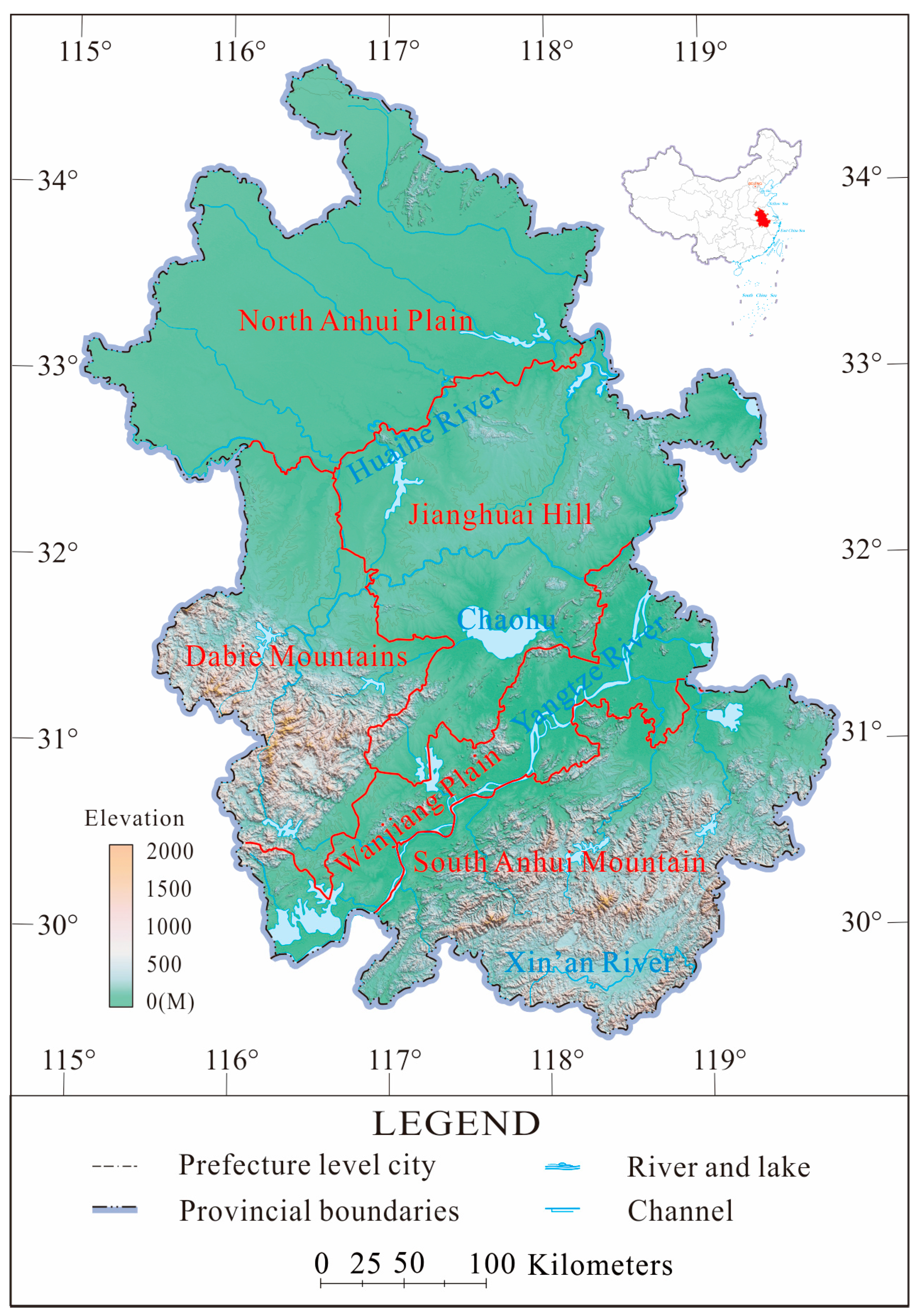
2.1. Study Area

The coordinate range of Anhui is from 114°54′ to 119°37′ in longitude, 29°41′ to 34°38′ in latitude, and has an administrative area of 140,100 km2, as shown in Figure 1. The landform is mainly composed of plains, hills, and low mountains, which are divided into five geomorphic areas: South Anhui Mountain, Jianghuai Hill, Dabie Mountains in West Anhui, Wanjiang Plain, and North Anhui Plain. A total of 416 km and 430 km of the Yangtze River and Huaihe River are located in the Anhui province, respectively [32]. Anhui’s climate is characterized by frequent intersections of warm and cold air, which is related to its location in the north-south climate transition zone. The special underlying surface conditions have poor adaptability to droughts and floods, making it an ecologically fragile area in China. At the same time, Anhui is a high-response area to climate change [33]. Its unique geographical location and climate have created outstanding agricultural regional characteristics. The crop types and multiple cropping indices in the north and south of the Huaihe River are significantly different. Anhui also is a major agricultural and the country’s main grain-producing province. The output of rice, wheat, and corn ranks highly in China [34].

2.2. Data Sets and Processing

2.2.1. Data Sets

Through the Google Earth Engine (GEE) platform (https://earthengine.google.com) the Landsat 30 m resolution satellite imagery data were downloaded. Landsat TM data was used before 2015, and Landsat OLI data was used in 2015 and 2020. All remote sensing images were processed on the GEE platform. It included the following processes: (1) all surface reflectance (SR) data were selected from the vegetation growth season (May–September) of each study year. (2) Data with less than 30% cloud cover were selected in Landsat images. The cloud-covered images were replaced and supplemented with images before and after the study to create the most usable pixel image composite. (3) The median function of GEE was used to generate a single image from the filtered image set. (4) The normalized difference vegetation index (NDVI), normalized difference construction index (NDBI), and modified normalized difference moisture index (MNDWI) were calculated for each image. The result was the best cloud-free image combination, combining NDVI, NDBI and MNDWI [35,36]. The main reason for choosing these three indices was that NDVI can reflect the distribution and intensity of prominent vegetation. MNDWI was modified from NDWI to enhance open water elements, while NDBI mainly highlighted built-up areas.
We then checked the Anhui Provincial Statistical Yearbook to obtain data on the planting range, output, and price of food. The change of ecological service value is a complex and dynamic process driven by the combination of natural and human factors. Influencing factors from three aspects were selected, namely nature, location, and socio-economic factors, as shown in Table 1. The elevation, slope, and aspect were calculated using SRTM 30 m obtained from the GEE platform. The distances to roads, residential areas, and water areas were obtained from a 1:250,000 national basic geographic database and processed in Arcgis10.2 (https://www.webmap.cn). Precipitation, NPP, population, GDP, soil erosion, and temperature factors were downloaded from the DataBox (https://www.databox.store).

2.2.2. Data Classification and Accuracy Assessment

According to China’s land use and land cover classification method and Anhui Province’s land use and land cover characteristics, classification included cultivated land, water area, grassland, unused land, forest land, and built-up land. The used maximum likelihood classification method (MLC) in the software ENVI 5.3, which is one of the most commonly used methods for remote sensing image classification, has the advantages of clear parameter interpretation capabilities, easy integration with prior knowledge, and simply and easily implemented algorithms. Then the land use data of Anhui Province every five years from 1990 to 2020 were obtained.
Some data in Anhui Province were used from three land surveys at Anhui Provincial Geomatics Center, in 1996, 2009 and 2020, from which 1410 sample data were collected. The sample data covered seven periods of land use data, and 70% of the data were selected for training samples, while the rest were used to verify the accuracy of the classification results. The overall classification accuracies in 1990 1995, 2000, 2005, 2010, 2015 and 2020 were 81.52%, 84.63%, 83.50%, 84.41%, 86.62%, 86.95%, and 89.23% respectively, with kappa coefficients of 0.778, 0.811, 0.796, 0.803, 0.822, 0.824, and 0.838, which met the basic conditions.

2.3. Methods

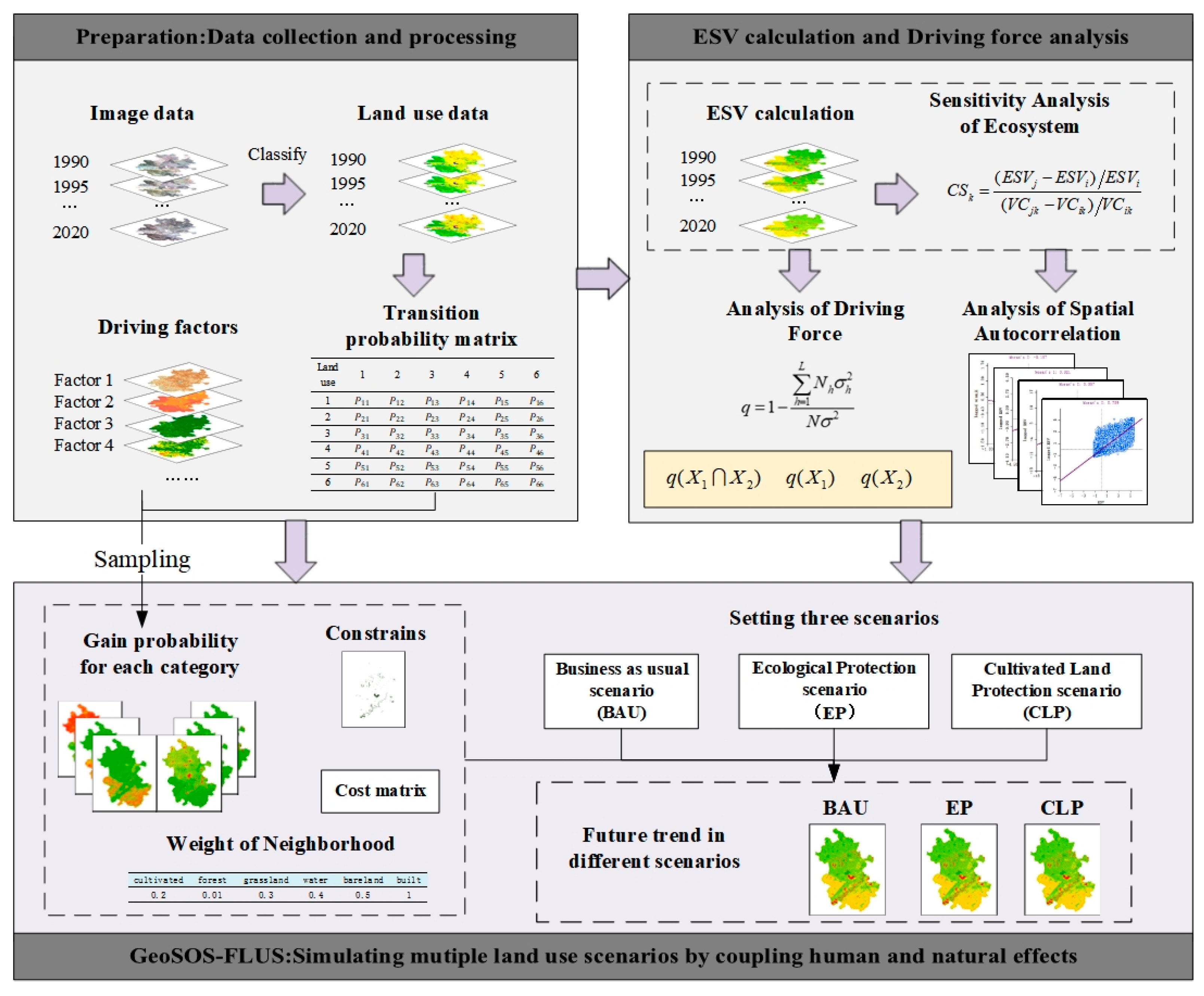
2.3.1. Technical Process

The detailed methods and flow chart are shown in Figure 2 with five steps:
(1)
Seven Landsat satellite images were obtained with atmospheric and topographic correction in 1990, 1995, 2000, 2005, 2010, 2015 and 2020 in GEE. The maximum likelihood classification method in ENVI5.3 was used to obtain Anhui land use data;
(2)
The ecosystem service value distribution is calculated in Anhui Province for seven periods based on the specific conditions of Anhui Province and China’s ecological service value equivalent factor method, and the spatiotemporal changes and ecological sensitivity of ESV are analyzed;
(3)
Spatial autocorrelation of ESV is analyzed from four scales: landform subdivision, county, town, and grid, and the spatial scale of the study is determined;
(4)
Driving factors and interactions between ESV factors are determined via Geodetector;
(5)
The ESV in 2030 is predicted using the GeoSOS-FLUS model for three scenarios.

2.3.2. Assessment of Ecosystem Service Value

Xie et al. [37] provided the national ESV equivalent table through questionnaire surveys combined with actual conditions. The ESV equivalent table was mainly suitable for national scale research. In regional scale research, there is bias. Therefore, Hu et al. [38] and Yu et al. [39] increased the ESV equivalent per unit area of construction land, and proposed the value equivalent coefficient of Anhui Province. In addition, Anhui Province mainly has dryland and paddy fields as its cultivated land types. Based on the third national land survey results of Anhui Province, the areas of these two types of land were almost the same. Therefore, the equivalent value of ecosystem services for cultivated land was calculated by the weighted average of the equivalent values of ecosystem services for dryland and paddy fields. Combining the previous three scholars, the equivalent table of ecological service value was adjusted to make it more suitable for estimating ecological service value in Anhui (Table 2).
Due to the differences in socio-economic development, Hu et al. [40,41] further adjusted the ESV coefficient of Anhui Province through some corrections. The final ESV evaluation model is expressed as follows:
E S V = i = 1 n R i × V i × Q × D × S
where R i and V i are the area and unit area ESV of land use type i . Q , D and S are the correction factor for grain production, regional development, and the resource scarcity, respectively.

2.3.3. Ecosystem Sensitivity Index

The ecosystem sensitivity index (ESI) is an analytical model that reflects the degree of correlation between ESV and its coefficient. It can test the elasticity of ESV to changes in the ecological service value coefficient within a period of time. The formula is as follows [42]:
C S c = ( E S V m E S V n ) / E S V n ( E V C m c E V C n c ) / E V C n c
where C S c is the ESI in the study area, E S V n and E S V m represent the ESV before and after adjustment, E V C m c is the ecological service value coefficient after adjustment, where it was set an increase of 50% on the original coefficient ( E V C n c ) before adjustment. From a theoretical perspective, C S is the change in ESV caused by every 1% change in E V C . If the dependent variable changes by more than 1, it indicates that it is more sensitive to changes and has obvious feedback, and the relationship between the two is full of elasticity. On the contrary, it is believed that the sensitivity between the two is poor and there is a lack of elasticity towards changes.

2.3.4. Global Moran’s Index

This paper chose the classic global Moran’s Index to test the spatial autocorrelation of ecosystem service values at four scales: landform division, county, town, and grid scales. When the global Moran’s I index is positive, ESV shows significant positive spatial autocorrelation, which exhibits aggregation characteristics. When the global Moran’s I index is negative, it shows negative spatial correlation, which exhibits spatial discreteness characteristics. The formula for the global Moran’s I is [1]:
I = [ i = 1 , j = 1 n W i j ( x i x ) ( x j x ) ] / [ T 2 i = 1 , j = 1 n W i j ]
T 2 = 1 n i = 1 n ( x i x ¯ ) 2
where n represents the number of research units, x i , x j represent ESV of area i and j , x ¯ represents the average ESV of all areas, and W i j represents the weight matrix with spatial binary symmetry.

2.3.5. Geodetector

Geodetector (http://www.geodetector.org/), developed by Wang’s team, is an analytical tool to analyze the spatial heterogeneity of geographical spatial element distribution [31]. Geodetector can detect the contribution of factors that affect ESV, study the driving mechanism of ESV changes, and analyze the relationship between influencing factors. The influence of each independent factor can be calculated via the following formula [43]:
q = 1 h = 1 L N h σ h 2 N σ 2
where q is a measure of the influence of independent variables, and the larger the value, the greater the influence, L is the stratification of ESV or influencing factors. N h and N are the number of units in the sub-regions h and study area respectively, σ h 2 and σ 2 are the variance of the layer and study area respectively.
Geodetector interaction detection was used to detect whether the interaction of two influencing factors was more obvious or the effect of a single factor, by comparing the sizes of q ( X 1 X 2 ) and q ( X 1 | X 2 ) . If the two-factor interaction has a greater impact than a single factor, it indicates that the two factors enhance the interpretation of ESV.
This paper selected 14 influencing factors from Table 1 to analyze the spatial heterogeneity of ESV. Geographic exploration was mainly used to identify its driving factors, and to reveal the degree and intensity of impact of key driving factors on ESV [44]. The natural breakpoint method in ArcGIS 10.3 software can be used to classify different influencing factors. This method is widely used in data classification based on the analysis of the intrinsic properties of the data to reduce within-group variance. According to previous studies, the influencing factors were divided into nine categories [45].

2.3.6. Multi-Scenario Simulation of ESV

The land use simulation model FLUS from Liu et al. [29] was used, which utilizes an artificial neural network model algorithm (ANN) to calculate the base period land use data and each driving factor data to obtain the suitability probability. The roulette selection method was also used to deal with the complexity and uncertainty of land use changes under the influence of multiple factors to finally obtain the prediction results [46].
Different land management policies and needs have formed different land use change scenarios. In 2020, Anhui Province had 83.2 million acres of cultivated land, accounting for 4.3% of the total cultivated land in China. According to the latest farmland protection policies in Anhui Province, the farmland cannot be reduced and should gradually increase to the numbers of land surveyed in the second national land survey. With reference to the Anhui Province Land Space Ecological Restoration Plan (2021–2035) and the Anhui Province Land Space Plan (2021–2035), in the indicator system of the planning text, the land use indicators were constrained, focusing on ecological protection and cultivated land protection on both sides. Therefore, this article set up simulation analysis scenarios for cultivated land protection and ecological protection [47]. The cultivated land protection scenario is mainly used to reduce the occupation of cultivated land by other land, especially the approval planning of construction land, and strictly avoids occupying cultivated land. The ecological protection scenario requires attention to the vegetation coverage of the land to avoid the loss of forest land and grassland [46]. The descriptions of the three simulation scenarios are shown in Table 3.
Before predicting land use and land cover in 2030, we first spatialized the LULCC driving factors from 2020 and selected the 14 driving factors introduced above. Then, using the land use and land cover data from 2020 as input data, the occurrence probability of each land use type in each pixel in Anhui Province was calculated. Then the probability matrix of land use transfer was calculated from 2010 to 2020. Finally, through simulation, the spatial distribution data of land use and land cover under the BAU, EP, and CLP scenarios in 2030 were obtained [1].

3. Results and Analysis

3.1. Changes in Land Use and Land Cover

The main land types in Anhui Province were cultivated land and forest land, accounting for approximately 60% and 20% of the province’s land area, respectively (Table 4). From 1990 to 2020, the cultivated land has been a decreasing trend with an about average 293 km2/year before 2015, followed by a significantly decreasing trend. Forest land and grassland increased slowly before 2010, and then gradually decreased. The water area decreased by 651.6 km2 from 1990 to 1995. From 1995 to 2015, the water area continued to increase to 7149.30 km2, 262.47 km2 more water area than that in 1990, and then between 2015 and 2020, it was decreased to 6827.81 km2. The unused land area of the land type is very small, only accounting for 0.01% of other land types. During the years from 1990 to 2020, it has decreased by 13.04 km2, and compared to the unused land area in 1990, it has decreased by 90.86%. Built-up land is the only one among the six land types that has been increasing year by year. From 1990 to 2020, it has increased by about 1.5 times when compared to 1990, and between 2010 and 2015, it has sharply increased by 1709.35 km2.

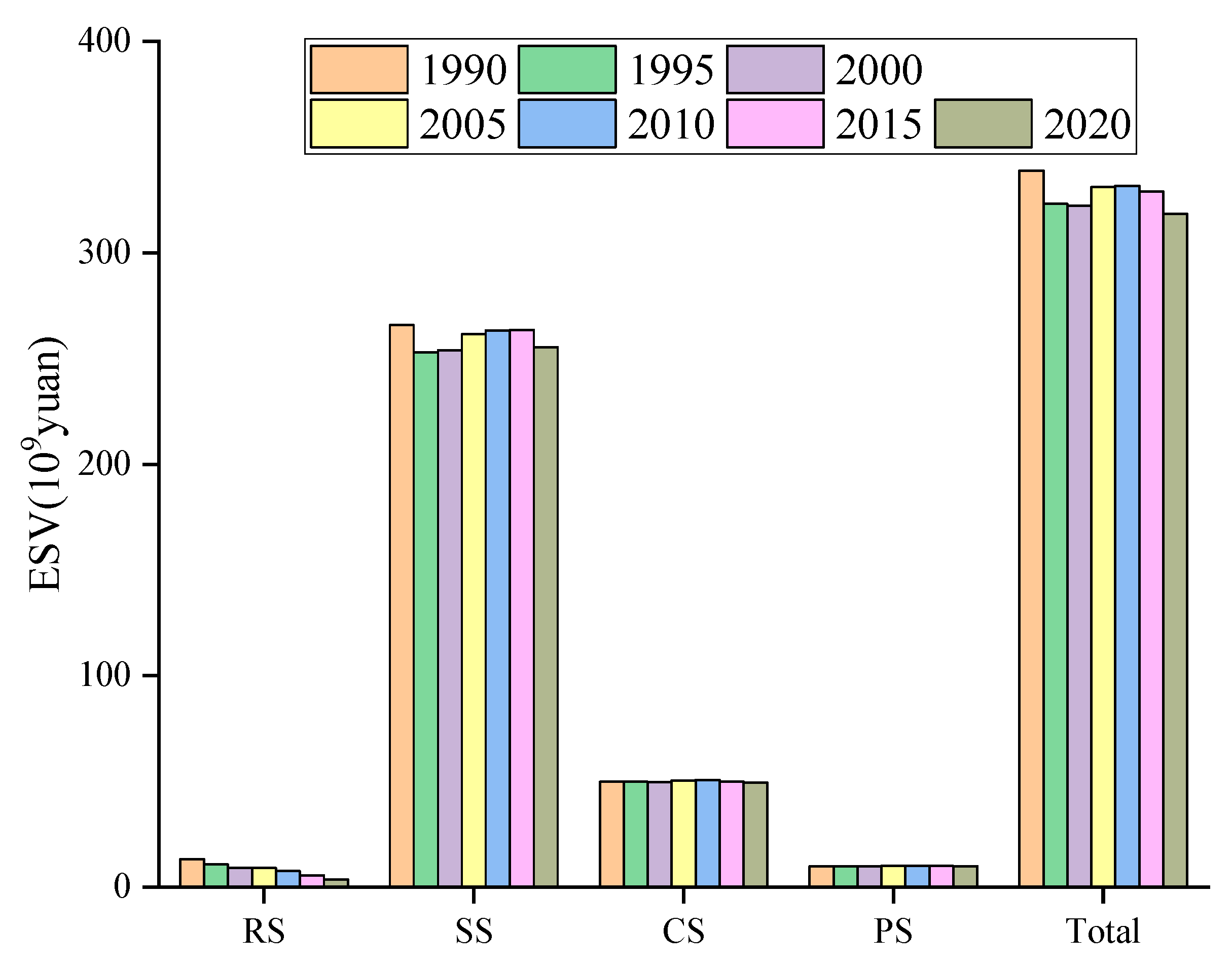
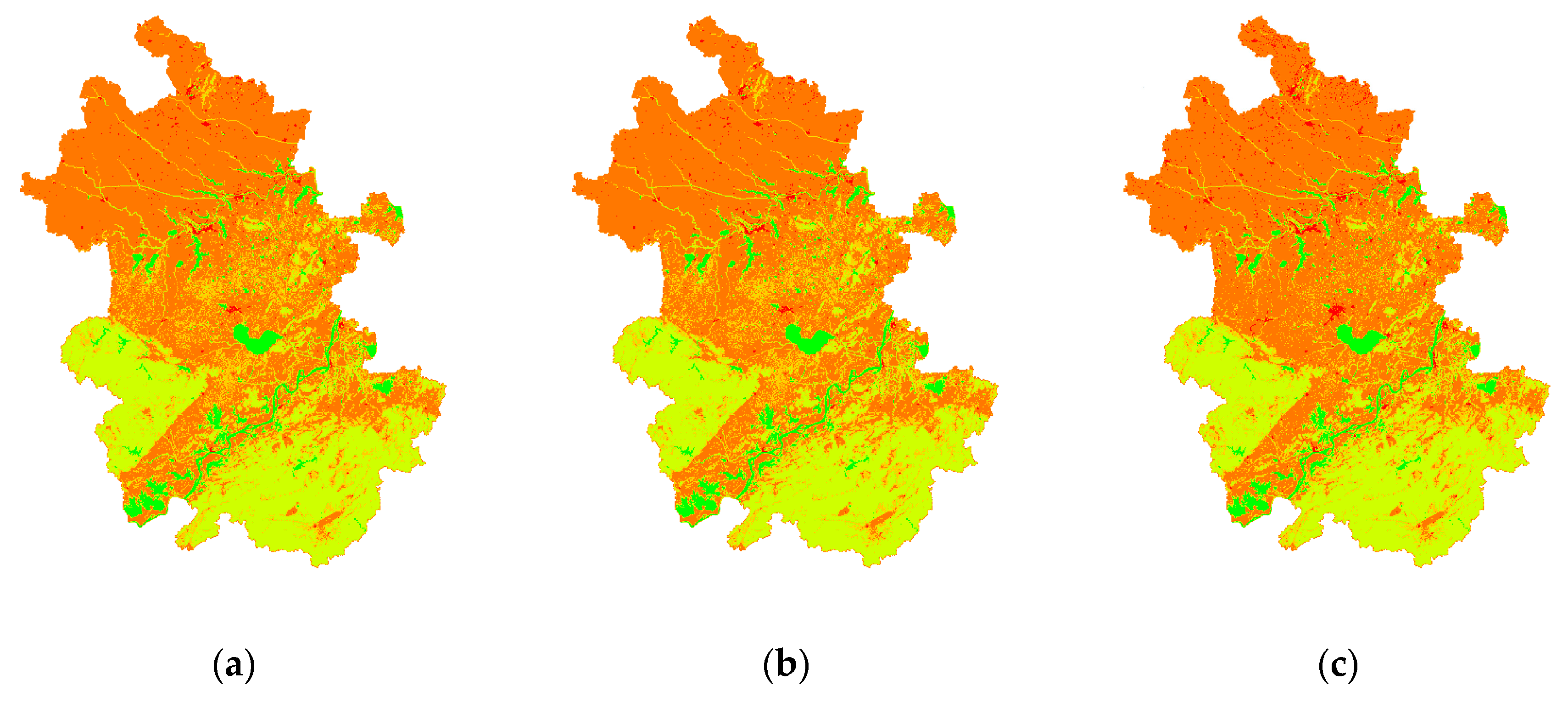
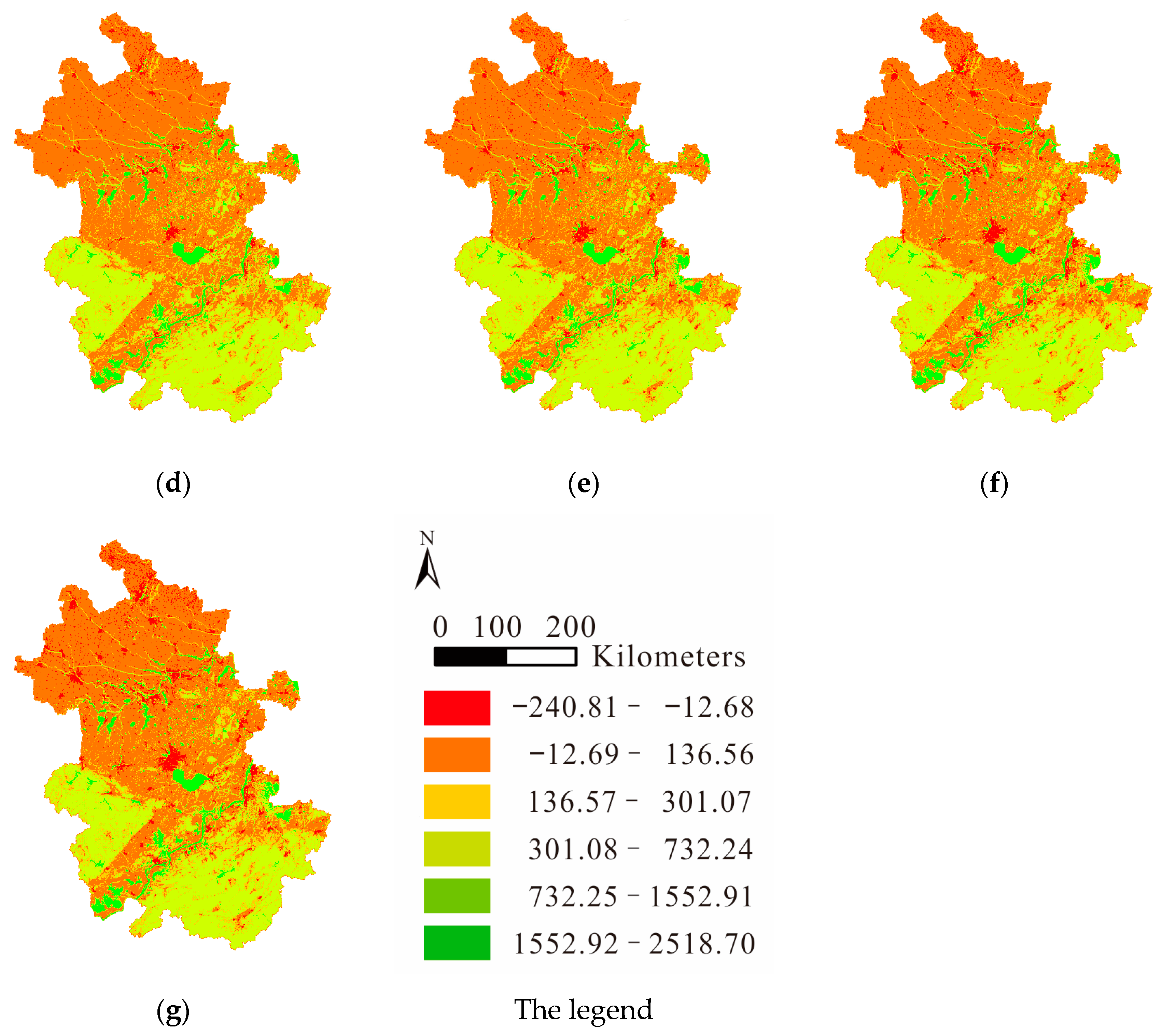
3.2. Spatiotemporal Changes of ESV from 1990 to 2020

Choosing an appropriate evaluation scale can elucidate the spatial clustering characteristics of ESV. This article chose GeoDa 1.20.0.10 software to calculate and analyze the spatial aggregation characteristics of ESV at four scales: landform, county, town, and grid level. The calculated Moran’s I and the drawn Moran scatter plot are shown in Figure 3. The results of the four scales were: −0.157, 0.321, 0.357, and 0.759, respectively. As the assessment unit of ESV decreases and the more obvious the spatial agglomeration characteristics are, it can be seen from Figure 4 that using a larger evaluation unit will filter out the differential information that originally existed in the ESV. Then, the Monte Carlo test method was used to test the significance of the statistics. The number of simulations was 999. Only the grid scale passed the test. Therefore, this paper chose the grid scale of 1 km × 1 km to study the distribution characteristics of ESV in Anhui Province.
The changes in ESV in Anhui Province over the past 30 years are shown in Table 5 and Figure 5. Overall, the cumulative value of ecosystem services has decreased by 2.045 billion yuan, which is approximately 6.03% of the ESV in 1990. From the perspective of individual ecological service functions, regulating services had the maximum ESV, approximately equal to 80% of the total ESV. Ranked second was supporting services accounting for about 15%, and provisioning services and cultural services having similar ecosystem service values. During this period, the ESV of provisioning services has been continuously decreasing by 72.7%. Regulating services, supporting services, and cultural services decreased in the first decade, increased in the second decade, and decreased again in the last decade. The overall decrease was 1.038 billion yuan, 41 million yuan and 5 million yuan, respectively.
By constructing a 1 km × 1 km grid in ArcGIS10.2, the calculation of ESV applied to the whole province is shown in Figure 6, where the spatial distribution and changing trends of ESV in Anhui Province were evaluated and analyzed. In terms of spatial distribution, the spatial pattern of ESV in the study area has changed little from 1990 to 2020, and there were clear regional differences, showing that the southern area was high and the northern area was low. The ESV of the Huaihe River Basin, Xin’an River Basin, Yangtze River Basin, and Chaohu Lake Basin was clearly higher; areas with high vegetation coverage in mountainous areas also have higher ESV. According to the zoning analysis of the five geomorphic scales in Figure 4, the order of ecosystem service value from high to low was: South Anhui Mountain, Jianghuai Hill, Dabie Mountains in West Anhui, Wanjiang Plain, and North Anhui Plain.

3.3. Ecosystem Sensitivity Analysis

According to Table 6, the ecological sensitivity index (ESI) of Anhui Province was all less than 1. This shows that the total ESV in the study area was inelastic to the ecological service function value coefficient (EVC). The EVC was more appropriate and the experimental results were credible. Overall, from high to low, they were: water area, forest land, cultivated land, grassland, built-up land, and unused land. Among them, the first two land types were relatively high, indicating that they were more sensitive to ESV in the province. In addition, at different times, the ESI changes in various categories were relatively small, with only the ESI of built-up land showing a continuous upward trend, indicating that the ESV sensitivity of construction land to EVC changes is gradually increasing.

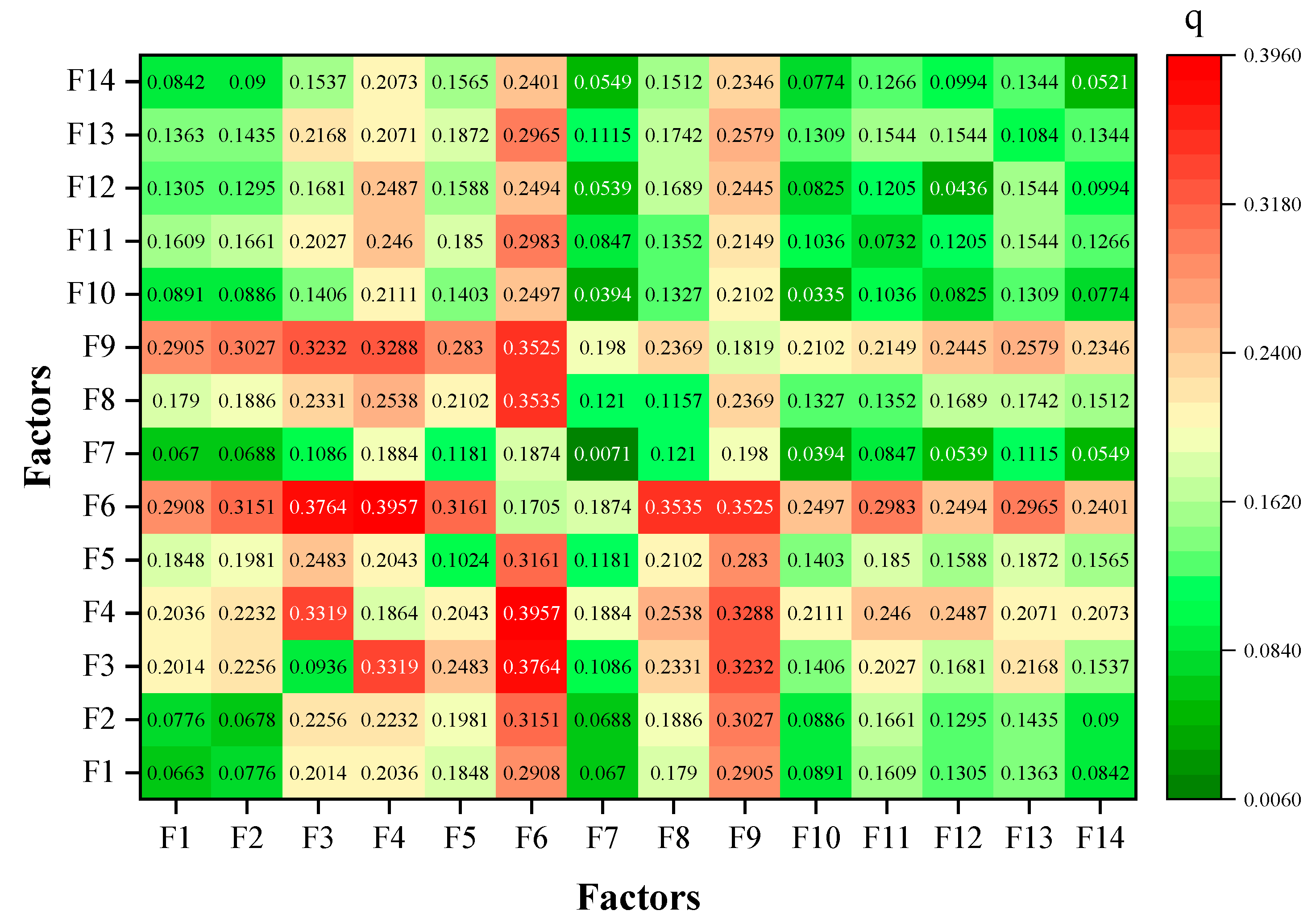
3.4. Driving Force of ESV

The distribution differences of ESV in Anhui Province were influenced by natural factors, location factors, and socio-economic factors. The explanatory power of each factor from large to small is: precipitation (F4), distance to intercity road (F9), net primary productivity, NPP (F6), distance to urban road (F8), population (F13), temperature (F5), aspect (F3), distance to settlement (F11), slope (F2), elevation (F1), GDP (F14), distance to water (F12), distance to railway (F10), and soil erosion (F7). Among them, the q value of F4 was 0.1864, which was the largest contribution rate to spatial differentiation of ESV. Among the natural factors, location factors and socio-economic factors, F4, F9 and F13 had the largest contribution rates respectively. From Figure 7, it can be seen that the interaction between the two factors was more obvious than the independent effect of the one factor, which also confirmed that the spatial differentiation results of ESV in Anhui Province were the result of the joint action of multiple driving factors. After interaction detection, the highest degree of interaction between (F6) and (F4) was 0.3957, which was more than twice the effect of a single factor. The top ten interaction degrees were: F4 and F6 (q = 0.3957), F3 and F4 (q = 0.3319), F6 and F2 (q = 0.3151), F6 and F3 (q = 0.3764), F6 and F5 (q = 0.3161), F8 and F6 (1 = 0.3535), F9 and F2 (q = 0.3027), F9 and F3 (q = 0.3232), F9 and F4 (q = 0.3288), and F9 and F6 (q = 0.3525).

3.5. Future Spatiotemporal ESV Pattern

The ESV in 2030 is predicted to be 30.482 billion yuan under the BAU scenario, 31.593 billion yuan under the EP scenario, and 30.701 billion yuan under the CLP scenario (Table 7). Compared with 2020, it was predicted to decrease by 1.359 billion yuan (−4.27%), 248 million yuan (−0.78%), and 1.140 billion yuan (−3.58%), respectively. Under the BAU scenario, Anhui Province has the highest loss of ESV, while under the EP scenario, Anhui Province has the least loss of ESV.
From the perspective of each individual ESV, under BAU scenario, there were losses in each individual ESV. In the first level category, PS and RS suffered losses of 384 million yuan and 817 million yuan, respectively, accounting for 88% of the total losses. Under the EP, the decreasing trend of ESV of primary type provisioning services, cultural services, regulating services, and supporting services did not reverse, but the loss was significantly lower than the other two scenarios. Among them, regulating services decreased by 157 million yuan, with the smallest reduction compared to other scenarios. Compared with the BAU scenario, the CLP scenario had smaller decreases in provisioning services and supporting services, which were 83 and 98 million yuan, respectively. Regulating services was the largest decrease among the three scenarios, with a decrease of 929 million yuan. Overall, ESV losses still existed in this scenario, but the degree of losses was relatively weakened compared to the BAU scenario.

4. Discussion

4.1. Impact of Land Use Change on ESV

The ESV is very sensitive to land cover and land use changes. A small change in land cover can cause a large change in ESV [48]. From Table 8, the main contributors to ESV in Anhui Province were forest and water areas, which were approximately 80% of the total ESV in Anhui Province. The third was cultivated land, accounting for approximately 18%. The ESV of unused land can be ignored. From 1990 to 2020, the ESV of cultivated land in Anhui was decreased by 518 million yuan, and the ESV of built-up land decreased by 1.528 billion yuan, ranking in the top two places in Anhui overall ESV reduction.
The built-up land in Anhui Province continued to increase, and the loss of cultivated land is serious, resulting in a continuous decrease in the ESV throughout the entire period from 1990 to 2020 (2.045 billion yuan, −6.03%) (Table 8). One of the reasons is that after more than 40 years of reform and opening up, Anhui Province has gradually completed its transformation from a traditional agricultural province to an emerging industrial province, with rapid population and economic growth. The urbanization rate was 17.9% in 1990 and reached 58.3% in 2020, and corresponding infrastructure, roads, and commerce must meet the development needs of urbanization. At the same time, farmers continue to work in cities, resulting in “non-cereal” and “non-agricultural” land use changes, and cultivated land is converted into built-up land. Another reason is that the economic benefits of built-up land are higher than traditional agriculture, so the cultivated land, water areas, and forest land are converted into construction land, ultimately reducing the ESV.
To sum up, land spatial planning should be formulated scientifically, and land use, economic development, and ecological protection should be coordinated and unified. With rapid urbanization, the red line of cultivated land should be strictly observed, and the distribution and area of construction land should be strictly reviewed and approved, so as to ultimately achieve an overall increase in ESV in Anhui Province.

4.2. Driving Mechanisms of ESV

The driving mechanism of ESV in Anhui Province is important for ecological management and the formulation of ecological models, and can also further explain the reasons for ecological problems [24]. Based on Figure 6 and Figure 8, the main factors affecting the spatial differentiation of ESV in Anhui Province with a q value greater than 0.1 were: precipitation (F4), distance to intercity roads (F9), net primary productivity (F6), distance to urban roads (F8), population (F13), and temperature (F5). It can be seen that the influence of natural factors is still in a dominant position, and the impacts of precipitation, net primary productivity, and temperature on ESV distribution were significant and consistent with previous studies [49]. Temperature and precipitation provide energy and water for plant growth, and within a certain range, the higher the temperature and precipitation, the greater the ESV [50]. Net primary productivity directly affects ESV by representing the status of plant growth. Of note are changes in distance to intercity roads, distance to urban roads, and population. Reflecting the impact of urbanization and agricultural activities on ecology, these three factors mainly affect land use. Through this article, we can understand the changing characteristics and influencing mechanisms of the ESV in the study area. In the optimization and protection of the ecosystem, we should consider the characteristics of different factors and the interactive and synergistic enhancement effect of the two factors, adopt a differentiated multi-regulatory strategy, choose a land use development model that is compatible with regional natural conditions and social and economic development levels, and avoid unreasonable or strong human interference and other factors that synergistically increase pressure on regional ecosystems [51].

4.3. Policy Recommendations for Land Use

It is very meaningful to predict the future land use pattern under different development goals in Anhui Province. Multiscenario simulation can provide suggestions and references for future development and planning [28]. The land management department of Anhui Province should adhere to the safety of cultivated land and ecological security. In the new round of land spatial planning, it should study the impact of changes in cultivated land and the internal factors of changes in ecological services, and scientifically divide ecological protection zones, basic farmland protection zones and urban development districts, and coordinate the relationship between the three. In addition, it is necessary to combine human activities, economic development, and other factors to achieve the coordination and unification of natural resources. The protection of cultivated land is the guarantee of China’s grain production, and cultivated land resources must be strictly protected. In addition, objective current conditions such as ecological damage and reduced environmental carrying capacity of land and resources must be improved in a targeted manner to control the scale of construction land.
In the context of urbanization and rapid economic development, the space for human activities continues to increase, which is directly reflected in the expansion of construction land. This requires the government management department to formulate corresponding policies to restrain it. Food security is very important at present. It is recommended that the government increases the protection of cultivated land and reduces the occupation of cultivated land by construction land. Secondly, ecological environment protection is the key to achieving sustainable economic development. It is recommended that the government reduces human activities in ecological reserves to avoid the destruction of natural ecology such as woodlands and waters.

4.4. Limitations

Based on Hu et al. [40], this paper further adjusted the ecological service value coefficient of Anhui Province. The ideas and methods of this article provide a reference for scientific study on the ESV, and also provide reasonable suggestions for sustainable economic development and natural resource management. However, this article still has some limitations. In the land use driving factors, data availability and accessibility were mainly considered, so it was not possible to comprehensively identify all the factors driving land use change. In the scenario simulation prediction, the Anhui Province Land Space Plan (2021–2035) and previous studies were mainly referred to [47]. The conversion parameters were subjective and need to be further improved later.

5. Conclusions

This article studied the spatiotemporal changes, sensitivity, spatial autocorrelation, and driving mechanisms of ESV in Anhui Province from 1990 to 2020. Based on the GeoSOS-FLUS model, the quantity and pattern characteristics of ESV in Anhui Province until 2030 were simulated. In summary, the main results are as follows:
(1)
From 1990 to 2020, the ESV in Anhui Province continued to decrease by 2.045 billion yuan (−6.03%). The ecosystem service value of various land use types in Anhui Province from large to small was water area, forest land, cultivated land, grassland, unused land, and construction land. The regional difference of ecosystem service value is obvious, according to the landform division, the order was from high to low in South Anhui Mountain, Jianghuai Hill, Dabie Mountains in West Anhui, Wanjiang Plain, and North Anhui Plain.
(2)
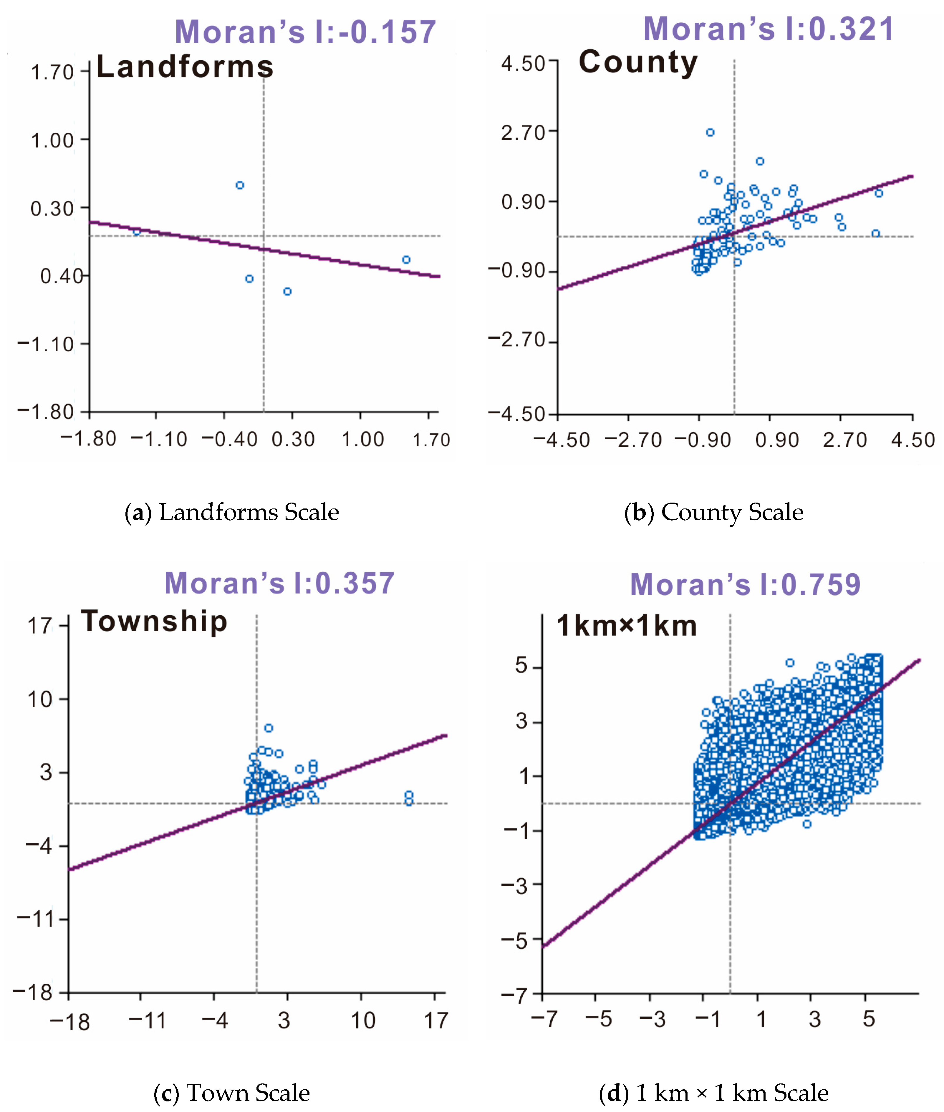
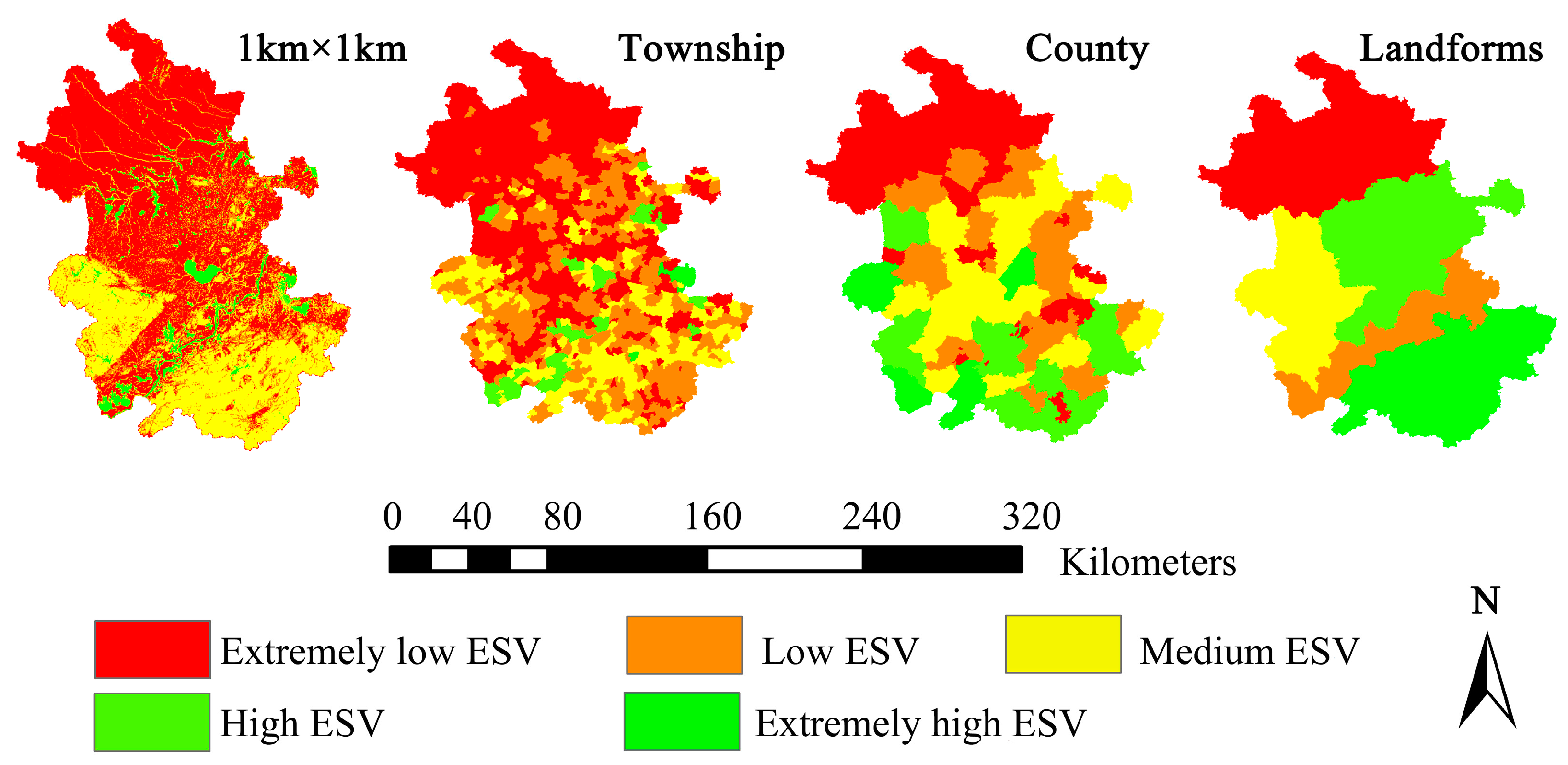
The spatial autocorrelation of ESV data at the four scales of landform subdivision, county, town, and grid scale in Anhui Province, Moran’s I was −0.157, 0.321, 0.357, and 0.759, respectively. Among the above four scales, the grid scale can better reflect the agglomeration characteristics of ESV.
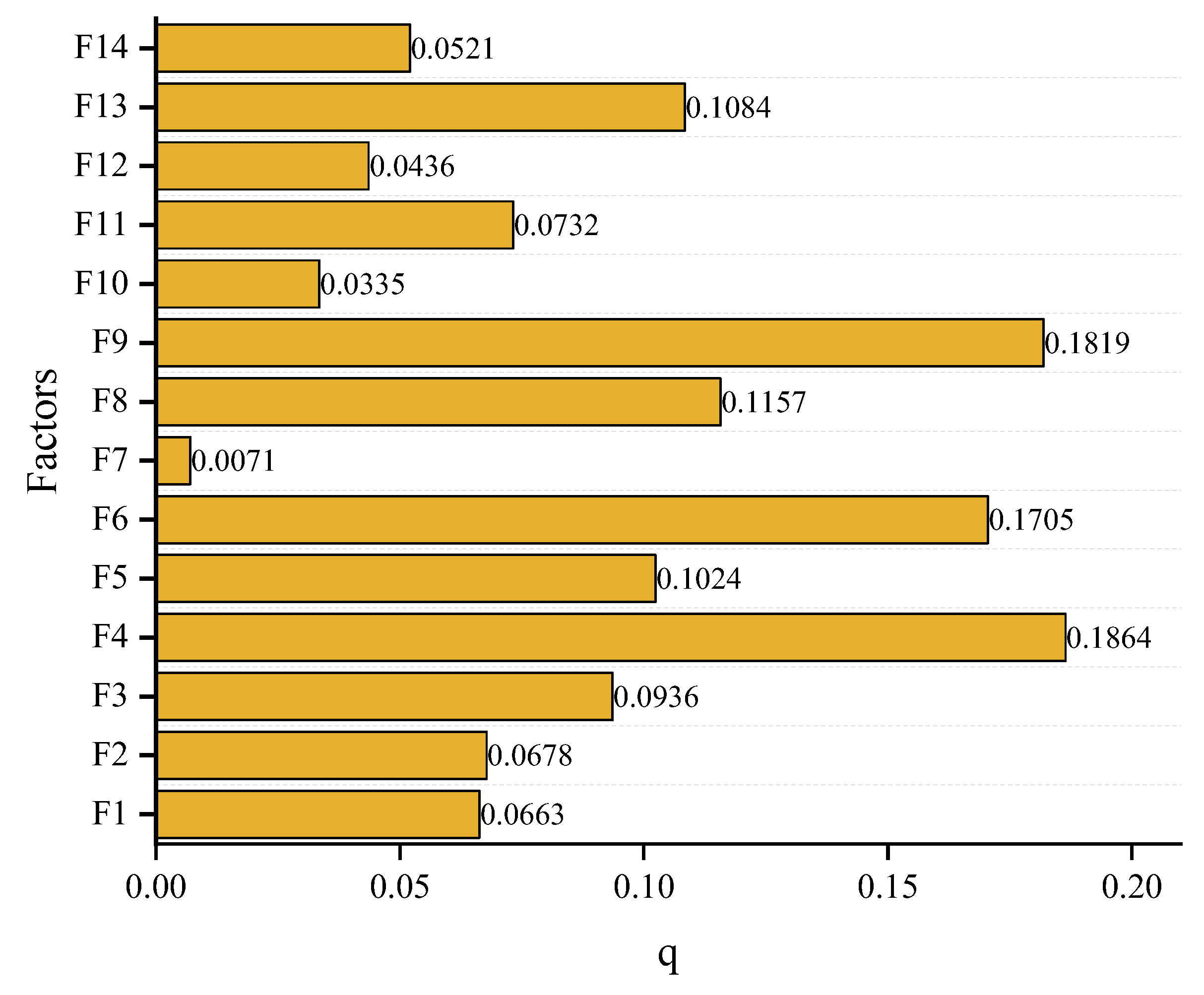
(3)
The detection results of the spatial differentiation driving factors of ESV, with a q values sorted as follows: precipitation (F4), distance to intercity road (F9), net primary productivity, NPP (F6), distance to urban road (F8), population (F13), temperature (F5), aspect (F3), distance to settlement (F11), slope (F2), elevation (F1), GDP (F14), distance to water (F12), distance to railway (F10), and soil erosion (F7).
(4)
The ESV was simulated in the three scenarios of BAU, EP, and CLP in 2030 with 30.482 billion yuan, 31.593 billion yuan, and 30.701 billion yuan, respectively. The ESV values of the three scenarios were decreased when compared to 2020: BAU (−1358 million yuan), EP (−248 million yuan), and CLP (−1139 million yuan).

Author Contributions

Conceptualization, L.Q. and S.J.; Methodology, L.Q.; Software, L.Q.; Validation, L.Q.; Data curation, J.C. and T.L.; Writing—original draft, L.Q.; Writing—review & editing, S.J.; Visualization, J.C. and T.L.; Supervision, S.J.; Funding acquisition, S.J.. All authors have read and agreed to the published version of the manuscript.

Funding

This work was supported by the Jiangsu Marine Science and Technology Innovation Project (Grant No.: JSZRHYKJ202202).

Data Availability Statement

Data available on request due to restrictions. The data presented in this study are available on request from the lead author, upon reasonable request.

Conflicts of Interest

The authors declare no conflict of interest.

References

  1. Liu, Y.; Hou, X.; Li, X.; Song, B.; Wang, C. Assessing and predicting changes in ecosystem service values based on land use/cover change in the Bohai Rim coastal zone. Ecol. Indic. 2020, 111, 106004. [Google Scholar] [CrossRef]
  2. Costanza, R.; dArge, R.; deGroot, R.; Farber, S.; Grasso, M.; Hannon, B.; Limburg, K.; Naeem, S.; Oneill, R.V.; Paruelo, J.; et al. The value of the world’s ecosystem services and natural capital. Nature 1997, 387, 253–260. [Google Scholar] [CrossRef]
  3. Rahman, M.M.; Szabó, G. Impact of Land Use and Land Cover Changes on Urban Ecosystem Service Value in Dhaka, Bangladesh. Land 2021, 10, 793. [Google Scholar] [CrossRef]
  4. Najibi, N.; Jin, S.G. Physical reflectivity and polarization characteristics for snow and ice-covered surfaces interacting with GPS signals. Remote Sens. 2013, 5, 4006–4030. [Google Scholar] [CrossRef]
  5. Tang, Z.; Sun, G.; Zhang, N.; He, J.; Wu, N. Impacts of Land-Use and Climate Change on Ecosystem Service in Eastern Tibetan Plateau, China. Sustainability 2018, 10, 467. [Google Scholar] [CrossRef]
  6. Li, S.; Zhang, Y.; Wang, Z.; Li, L. Mapping human influence intensity in the Tibetan Plateau for conservation of ecological service functions. Ecosyst. Serv. 2018, 30, 276–286. [Google Scholar] [CrossRef]
  7. Xi, H.; Cui, W.; Cai, L.; Chen, M.; Xu, C. Evaluation and Prediction of Ecosystem Service Value in the Zhoushan Islands Based on LUCC. Sustainability 2021, 13, 2302. [Google Scholar] [CrossRef]
  8. Li, Z.; Sun, Z.; Tian, Y.; Zhong, J.; Yang, W. Impact of Land Use/Cover Change on Yangtze River Delta Urban Agglomeration Ecosystem Services Value: Temporal-Spatial Patterns and Cold/Hot Spots Ecosystem Services Value Change Brought by Urbanization. Int. J. Environ. Res. Public Health 2019, 16, 123. [Google Scholar] [CrossRef] [PubMed]
  9. An, G.Q.; Han, Y.X.; Gao, N.; Lanshu, J.I.; Gao, H.B.; Tan, X.Q.; Xu, Y.T. Quantity and equilibrium of ecosystem service value and their spatial distribution patterns in Shandong Province. China Popul. Resour. Environ. 2021, 31, 9–18. [Google Scholar] [CrossRef]
  10. Shi, Y.; Wang, R.; Huang, J.; Yang, W. An analysis of the spatial and temporal changes in Chinese terrestrial ecosystem service functions. Chin. Sci. Bull. 2012, 57, 2120–2131. [Google Scholar] [CrossRef]
  11. Su, S.; Xiao, R.; Jiang, Z.; Zhang, Y. Characterizing landscape pattern and ecosystem service value changes for urbanization impacts at an eco-regional scale. Appl. Geogr. 2012, 34, 295–305. [Google Scholar] [CrossRef]
  12. Makwinja, R.; Kaunda, E.; Mengistou, S.; Alamirew, T. Impact of land use/land cover dynamics on ecosystem service value—A case from Lake Malombe, Southern Malawi. Environ. Monit. Assess. 2021, 193, 492. [Google Scholar] [CrossRef]
  13. Xie, G.; Zhang, C.; Zhang, L.; Chen, W.; Li, S. Improvement of the Evaluation Method for Ecosystem Service Value Based on Per Unit Area. J. Nat. Resour. 2015, 30, 1243–1254. [Google Scholar] [CrossRef]
  14. Xie, G.D.; Zhen, L.; Lu, C.X.; Xiao, Y.; Chen, C. Expert Knowledge Based Valuation Method of Ecosystem Services in China. J. Nat. Resour. 2008, 23, 0911–0919. [Google Scholar]
  15. Xie, G.D.; Zhang, C.X.; Zhang, C.S.; Xiao, Y.; Lu, C.X. The value of ecosystem services in China. Resour. Sci. 2015, 37, 1740–1746. [Google Scholar]
  16. Xie, G.; Xiao, Y. Review of agro-ecosystem services and their values. Chin. J. Eco-Agric. 2013, 21, 645–651. [Google Scholar] [CrossRef]
  17. Pan, J.H.; Zhang, W.; Li, J.F.; Wen, Y.; Wang, C.J. Spatial distribution characteristics of air pollutants in major cities in China during the period of wide range haze pollution. Chin. J. Ecol. 2014, 33, 3423–3431. [Google Scholar] [CrossRef]
  18. Kumari, M.; Sarma, K.; Sharma, R. Using Moran’s I and GIS to study the spatial pattern of land surface temperature in relation to land use/cover around a thermal power plant in Singrauli district, Madhya Pradesh, India. Remote Sens. Appl. Soc. Environ. 2019, 15, 100239. [Google Scholar] [CrossRef]
  19. Zhang, B.; Wang, Y.; Li, J.; Zheng, L. Degradation or Restoration? The Temporal-Spatial Evolution of Ecosystem Services and Its Determinants in the Yellow River Basin, China. Land 2022, 11, 863. [Google Scholar] [CrossRef]
  20. Chi, J.; Xu, G.; Yang, Q.; Liu, Y.; Sun, J. Evolutionary characteristics of ecosystem services and ecological risks at highly developed economic region: A case study on Yangtze River Delta, China. Environ. Sci. Pollut. R 2022, 30, 1152–1166. [Google Scholar] [CrossRef]
  21. Hoque, M.Z.; Ahmed, M.; Islam, I.; Cui, S.; Xu, L.; Prodhan, F.A.; Ahmed, S.; Rahman, M.A.; Hasan, J. Monitoring Changes in Land Use Land Cover and Ecosystem Service Values of Dynamic Saltwater and Freshwater Systems in Coastal Bangladesh by Geospatial Techniques. Water 2022, 14, 2293. [Google Scholar] [CrossRef]
  22. Akhtar, M.; Zhao, Y.; Gao, G. An analytical approach for assessment of geographical variation in ecosystem service intensity in Punjab, Pakistan. Environ. Sci. Pollut. Res. Int. 2021, 28, 38145–38158. [Google Scholar] [CrossRef]
  23. Chen, R.; Yang, C.; Yang, Y.; Dong, X.Z. Spatial-temporal evolution and drivers of ecosystem service value in the Dongting Lake Eco-economic Zone, China. Chin. J. Appl. Ecol. 2022, 33, 169–179. [Google Scholar] [CrossRef]
  24. Song, F.; Su, F.; Mi, C.; Sun, D. Analysis of driving forces on wetland ecosystem services value change: A case in Northeast China. Sci. Total Environ. 2021, 751, 141778. [Google Scholar] [CrossRef]
  25. Pan, S.; Liang, J.; Chen, W.; Li, J.; Liu, Z. Gray Forecast of Ecosystem Services Value and Its Driving Forces in Karst Areas of China: A Case Study in Guizhou Province, China. Int. J. Environ. Res. Public. Health 2021, 18, 2404. [Google Scholar] [CrossRef]
  26. Yu, Y.; Yu, M.; Lin, L.; Chen, J.; Li, D.; Zhang, W.; Cao, K. National Green GDP Assessment and Prediction for China Based on a CA-Markov Land Use Simulation Model. Sustainability 2019, 11, 576. [Google Scholar] [CrossRef]
  27. Wu, C.; Chen, B.; Huang, X.; Dennis Wei, Y.H. Effect of land-use change and optimization on the ecosystem service values of Jiangsu province, China. Ecol. Indic. 2020, 117, 106507. [Google Scholar] [CrossRef]
  28. Lou, Y.; Yang, D.; Zhang, P.; Zhang, Y.; Song, M.; Huang, Y.; Jing, W. Multi-Scenario Simulation of Land Use Changes with Ecosystem Service Value in the Yellow River Basin. Land 2022, 11, 992. [Google Scholar] [CrossRef]
  29. Liu, X.; Liang, X.; Li, X.; Xu, X.; Ou, J.; Chen, Y.; Li, S.; Wang, S.; Pei, F. A future land use simulation model (FLUS) for simulating multiple land use scenarios by coupling human and natural effects. Landsc. Urban Plan. 2017, 168, 94–116. [Google Scholar] [CrossRef]
  30. Liang, X.; Liu, X.; Li, X.; Chen, Y.; Tian, H.; Yao, Y. Delineating multi-scenario urban growth boundaries with a CA-based FLUS model and morphological method. Landsc. Urban Plan. 2018, 177, 47–63. [Google Scholar] [CrossRef]
  31. Wang, J.; Xu, C. Geodetector: Principle and prospective. Acta Geogr. Sin. 2017, 72, 116–134. [Google Scholar] [CrossRef]
  32. Wang, D.; Wang, S.; Wu, J.; Zhou, L. Research on Ecological Service Value of Anhui Province Based on Land Use Change. Bull. Soil Water Conserv. 2015, 35, 0242–0247. [Google Scholar] [CrossRef]
  33. Wa, S.; Xu, H.-M.; Wa, D.-Y. Projection of vegetation net primary productivity based on CMIP5 models in Anhui province. Clim. Change Res. 2018, 14, 266–274. [Google Scholar] [CrossRef]
  34. Wang, F.; Wang, Z.; Zhang, Y. Spatio-temporal variations in vegetation Net Primary Productivity and their driving factors in Anhui Province from 2000 to 2015. Acta Ecol. Sin. 2018, 38, 2754–2767. [Google Scholar] [CrossRef]
  35. Szabó, S.; Gácsi, Z.; Balázs, B. Specific features of NDVI, NDWI and MNDWI as reflected in land cover categories. Landsc. Environ. 2016, 10, 194–202. [Google Scholar] [CrossRef]
  36. Zhang, D.D.; Zhang, L. Land Cover Change in the Central Region of the Lower Yangtze River Based on Landsat Imagery and the Google Earth Engine: A Case Study in Nanjing, China. Sensors 2020, 20, 91. [Google Scholar] [CrossRef]
  37. Xie, G.; Xiao, Y.; Zhen, L.; Lu, C. Study on ecosystem services value of food production in China. Chin. J. Eco-Agric. 2005, 13, 10–13. [Google Scholar]
  38. Hu, S.; Chen, L.; Li, L.; Wang, B.; Yuan, L.; Cheng, L.; Yu, Z.; Zhang, T. Spatiotemporal Dynamics of Ecosystem Service Value Determined by Land-Use Changes in the Urbanization of Anhui Province, China. Int. J. Environ. Res. Public Health 2019, 16, 5104. [Google Scholar] [CrossRef]
  39. Kang, Y.; Cheng, C.; Liu, X.; Zhang, F.; Li, Z.; Lu, S. An ecosystem services value assessment of land-use change in Chengdu: Based on a modification of scarcity factor. Phys. Chem. Earth Parts A/B/C 2019, 110, 157–167. [Google Scholar] [CrossRef]
  40. Yang, Y.; Yang, H.; Li, Y.; Li, M. Spatial-temporal Change Analysis of Ecosystem Service Value in Nanchang City Based on Land Use. J. Gansu Sci. 2022, 34, 23–27. [Google Scholar] [CrossRef]
  41. Hu, S.; Chen, L.; Li, L.; Zhang, T.; Yuan, L.; Cheng, L.; Wang, J.; Wen, M. Simulation of Land Use Change and Ecosystem Service Value Dynamics under Ecological Constraints in Anhui Province, China. Int. J. Environ. Res. Public Health 2020, 17, 4228. [Google Scholar] [CrossRef]
  42. Kreuter, U.P.; Harris, H.G.; Matlock, M.D.; Lacey, R.E. Change in ecosystem service values in the San Antonio area, Texas. Ecol. Econ. 2001, 39, 333–346. [Google Scholar] [CrossRef]
  43. Zhang, R.; Li, C.; Yao, S.; Li, W. Study on the change factors of construction land in Taiyuan by integrating geographic detector and geographically weighted regression. Bull. Surv. Mapp. 2022, 2022, 106–109. [Google Scholar] [CrossRef]
  44. Liu, C.; Li, W.; Zhu, G.; Zhou, H.; Yan, H.; Xue, P. Land Use/Land Cover Changes and Their Driving Factors in the Northeastern Tibetan Plateau Based on Geographical Detectors and Google Earth Engine: A Case Study in Gannan Prefecture. Remote Sens. 2020, 12, 3139. [Google Scholar] [CrossRef]
  45. Zhao, R.; Zhan, L.; Zhou, L.; Zhang, J. Identification of driving factors of PM2.5 based on geographic detector combined with geographically weighted ridge regression. Ecol. Environ. Sci. 2022, 31, 307–317. [Google Scholar] [CrossRef]
  46. Chen, L.T.; Cai, H.S.; Zhang, T.; Zhang, X.L.; Zeng, H. Land use multi-scenario simulation analysis of Rao River Basin Based on Markov-FLUS model. Acta Ecol. Sin. 2022, 42, 3947–3958. [Google Scholar] [CrossRef]
  47. Zhang, X.; Lu, L.; Yu, H.; Zhang, X.; Li, D. Multi-scenario simulation of the impacts of land-use change on ecosystem service value on the Qinghai-Tibet Plateau. Chin. J. Ecol. 2021, 40, 887–898. [Google Scholar] [CrossRef]
  48. Pan, N.; Guan, Q.; Wang, Q.; Sun, Y.; Li, H.; Ma, Y. Spatial Differentiation and Driving Mechanisms in Ecosystem Service Value of Arid Region: A case study in the middle and lower reaches of Shule River Basin, NW China. J. Clean. Prod. 2021, 319, 128718. [Google Scholar] [CrossRef]
  49. Xie, L.; Wang, H.; Liu, S. The ecosystem service values simulation and driving force analysis based on land use/land cover: A case study in inland rivers in arid areas of the Aksu River Basin, China. Ecol. Indic. 2022, 138, 108828. [Google Scholar] [CrossRef]
  50. Wang, R.S.; Pan, H.Y.; Liu, Y.H.; Tang, Y.P.; Zhang, Z.F.; Ma, H.J. Evolution and driving force of ecosystem service value based on dynamic equivalent in Leshan City. Acta Ecol. Sin. 2022, 42, 76–90. [Google Scholar] [CrossRef]
  51. Li, K.M.; Wang, X.Y.; Yao, L.L.; Yun, S. Spatio-temporal change and driving factor analysis of ecosystem service value in the Beijing-Tianjin-Hebei Region. J. Environ. Eng. Technol. 2022, 12, 1114–1122. [Google Scholar] [CrossRef]
Figure 1. Location and Topographic Map of Anhui Province.
Remotesensing 16 00269 g001
Figure 2. Flowchart of study scheme.
Remotesensing 16 00269 g002
Figure 3. Moran scatter plot of spatial autocorrelation analysis at different spatial scales.
Remotesensing 16 00269 g003
Figure 4. Distribution of ESV at four scales.
Remotesensing 16 00269 g004
Figure 5. Changes in the ESV from 1990 to 2020.
Remotesensing 16 00269 g005
Figure 6. Changes in the distribution of ESV. The distribution of ESV in 1990 (a). The distribution of ESV in 1995 (b). The distribution of ESV in 2000 (c). The distribution of ESV in 2005 (d). The distribution of ESV in 2010 (e). The distribution of ESV in 2015 (f). The distribution of ESV in 2020 (g).
Remotesensing 16 00269 g006aRemotesensing 16 00269 g006b
Figure 7. Single-factor detection and two-factor interaction detection results.
Remotesensing 16 00269 g007
Figure 8. Contribution Value of ESV Driving Factors in Anhui Province.
Remotesensing 16 00269 g008
Table 1. Selected ESV driving factors.
Factor TypesDriving FactorsTimeSignsUnits
Natural factorselevation2000, 2015F1m
slope2000, 2015F2°
aspect2000, 2015F3°
precipitation1900, 1995, 2000, 2005, 2010, 2015, 2020F4mm
temperature1900, 1995, 2000, 2005, 2010, 2015, 2020F5°C
NPP1900, 1995, 2000, 2005, 2010, 2015, 2020F6/
soil erosion1900, 1995, 2000, 2005, 2010, 2015, 2020F7Multi-class
Locational factorsdistance to urban road2010, 2015, 2020F8km
distance to intercity road2010, 2015, 2020F9km
distance to railway2010, 2015, 2020F10km
distance to settlement2010, 2015, 2020F11km
distance to water2010, 2015, 2020F12km
Social and economic factorspopulation1900, 1995, 2000, 2005, 2010, 2015, 2020F13people/km2
GDP1900, 1995, 2000, 2005, 2010, 2015, 2020F1410,000 yuan/km2
Table 2. ESV coefficient per unit area of different land types in Anhui Province (yuan/hm2).
Ecosystem ServicesTypeCultivated LandForest LandGrass LandWater AreaBuilt-Up LandUnused Land
Provisioning services
(PS)
Food production (FP)1899.63498.54653.271375.3017.190.00
Raw material production (RMP)421.181134.62962.71395.400.000.00
Water supply (WS)−2243.45584.50532.9314,251.50−12,910.580.00
Regulating services
(RS)
Gas regulation (GR)1530.023730.493386.661323.72−4160.2734.38
Climate regulation (CR)799.3911,174.278956.613936.780.000.00
Hydrological regulation (HR)2570.088148.626567.04175,762.740.0051.57
Environmental purification (EP)232.083317.902956.889541.11−4229.03171.91
Supporting services
(SS)
Soil formation and retention (SR)893.944555.674125.891598.7834.3834.38
Maintain nutrient cycling (MNC)266.46343.82309.44120.340.000.00
Biodiversity protection (BP)292.254143.083747.684383.75584.5034.38
Cultural services
(CS)
Recreation and culture (RC)128.931822.271650.353249.1417.1917.19
Total6790.5239,453.7833,849.46215,938.55−20,646.62343.82
Table 3. Description of Three Different Simulation Scenarios.
ScenariosScenario Description
Business As Usual
(BAU)
Without considering the constraining effects of any planning policies and restricted areas on surface cover and land use changes, future scenario simulations were conducted using the laws of land use and land cover conversion in Anhui Province from 2010 to 2020.
Cultivated Land Protection
(CLP)
The probability of the transfer of cultivated land to construction land is reduced by 80%, and except for unused land, other land types are reduced by 40%.
Ecological Protection
(EP)
Considering the ecological, agricultural, urban, and other land use structures, the probability of transferring forest and grassland to built-up land will be reduced by 50%, cultivated land to built-up land will be reduced by 30%, and cultivated land and grassland to forest land will be increased by 30%.
Table 4. LULCC in Anhui Province from 1990 to 2020.
LULCCArea/km2
Proportion/%
1990199520002005201020152020
Cultivated land91,928.5190,954.4789,632.0487,453.2085,612.3184,594.1884,294.27
65.62%64.92%63.98%62.42%61.11%60.38%60.17%
Forest land27,303.6027,619.9527,397.0528,063.1328,207.0127,705.1127,606.61
19.49%19.71%19.56%20.03%20.13%19.78%19.70%
Grassland8927.559037.598909.999457.369667.869247.348936.76
6.37%6.45%6.36%6.75%6.90%6.60%6.38%
Water area6886.836235.236434.696766.476916.587149.306827.81
4.92%4.45%4.59%4.83%4.94%5.10%4.87%
Unused land14.3517.4211.515.662.701.191.31
0.01%0.01%0.01%0.00%0.00%0.00%0.00%
Built-up land5039.156235.347714.728354.199693.5311,402.8812,433.24
3.60%4.45%5.51%5.96%6.92%8.14%8.87%
Table 5. Changes in the ESV from 1990 to 2020 (billion yuan).
1990199520002005201020152020
Provisioning services
(PS)
1.3231.0730.9050.9000.7580.5540.361
Regulating services
(RS)
26.58525.29725.40026.15726.33126.35225.547
Supporting services
(SS)
4.9904.9814.9525.0505.0715.0014.949
Cultural services
(CS)
0.9890.9740.9731.0021.0111.0010.984
Total33.88632.32432.23033.10833.17132.90731.841
Table 6. Anhui Province Ecosystem Service Value Ecosystem Sensitivity Index.
1990199520002005201020152020
Cultivated Land0.18430.19120.18890.17940.17540.17470.1799
Forest Land0.31810.33730.33550.33450.33570.33240.3423
Grass Land0.08920.09470.09360.09670.09870.09520.0951
Water Area0.43910.41670.43130.44150.45060.46940.4634
Unused Land0.00000.00000.00000.00000.00000.00000.0000
Built-Up Land0.03070.03980.04940.05210.06040.07160.0807
Table 7. Ecological Service Value under Different Scenario Simulations (billion yuan).
20202030 (BAU)2030 (EP)2030 (CLP)
Proportion of Change (%)
Provisioning services
(PS)
0.36−0.020.290.28
−106.37%−19.11%−22.99%
Regulating services
(RS)
25.5524.7325.3924.62
−3.20%−0.61%−3.64%
Supporting services
(SS)
4.954.824.934.85
−2.61%−0.36%−1.98%
Cultural services
(CS)
0.980.9550.980.955
−2.95%−0.41%−2.95%
Total31.8430.4831.5930.70
−4.27%−0.78%−3.58%
Table 8. Changes in the ESV of each land type from 1990 to 2030.
TypeESV/Billion Yuan
Proportion/%
19901995200020052010201520202030
(BAU)
2030 (EP)2030 (CLP)
Cultivated Land6.256.186.095.945.825.755.735.625.835.87
18.43%19.12%18.90%17.94%17.54%17.47%17.99%18.44%18.45%19.13%
Forest Land10.7810.9010.8111.0811.1410.9410.9010.6310.9210.65
31.81%33.73%33.55%33.45%33.57%33.23%34.23%34.86%34.56%34.69%
Grass Land3.023.063.023.203.273.133.032.802.882.78
8.92%9.47%9.36%9.67%9.87%9.52%9.51%9.19%9.12%9.07%
Water Area14.8813.4713.9014.6214.9515.4514.7514.5414.9814.09
43.91%41.67%43.13%44.14%45.06%46.94%46.34%47.71%47.40%45.90%
Unused Land0.000.000.000.000.000.000.000.000.000.00
0.00%0.00%0.00%0.00%0.00%0.00%0.00%0.00%0.00%0.00%
Built-Up Land−1.04−1.29−1.59−1.73−2.00−2.36−2.57−3.11−3.01−2.70
−3.07%−3.98%−4.94%−5.21%−6.04%−7.16%−8.07%−10.20%−9.53%−8.79%
Total33.8932.3232.2333.1133.1732.9131.8430.4831.5930.70
Disclaimer/Publisher’s Note: The statements, opinions and data contained in all publications are solely those of the individual author(s) and contributor(s) and not of MDPI and/or the editor(s). MDPI and/or the editor(s) disclaim responsibility for any injury to people or property resulting from any ideas, methods, instructions or products referred to in the content.

