Analysis of the Substantial Growth of Water Bodies during the Urbanization Process Using Landsat Imagery—A Case Study of the Lixiahe Region, China

Abstract

In the process of urbanization, water bodies bear considerable anthropogenic pressure, resulting in a reduction of their surface area in most instances. Nevertheless, in contrast to many other regions, the Lixiahe region in Jiangsu Province, located in China’s eastern plain, has experienced a continuous expansion of water bodies over the past few decades amid rapid urbanization. Using Landsat images spanning from 1975 to 2023, this study analyzed changes in water resources and the growth of impervious surfaces during urbanization. The findings revealed that the area of impervious surfaces in the region increased from 227.1 km² in 1975 to 1883.1 km² in 2023. Natural wetland suffered significant losses, declining from 507.2 km² in 1975 to near disappearance by the year 2000, with no significant recovery observed thereafter. Simultaneously, the water area expanded from 459.3 km² in 1975 to 2373.1 km² in 2023, primarily propelled by the significant contribution of aquaculture ponds, accounting for 2175.0 km² or 91.7% of the total water area. Driver analysis revealed that these changes were found to be influenced by factors such as population, economy, demand, and policies. However, alongside the economic development brought by urbanization, negative impacts such as lake shrinkage, eutrophication, and increased flood risks have emerged. The Lixiahe region, as a relatively underdeveloped part of Jiangsu Province, faces the challenge of striking a balance between economic growth and environmental conservation.

1. Introduction

Water is a vital and precious resource that forms the foundation of all life and plays a critical role in the Earth’s ecological cycle. With the development of urbanization, human activities are increasingly affecting nature, leading to water quality deterioration, frequent floods, soil erosion, and loss of biodiversity, among other water ecological issues [1,2,3,4,5]. As a result, water resource security is continuously under pressure. Therefore, in the context of rapid urbanization, accurate monitoring and evaluation of water is necessary for water resource management.

In the past several decades, satellite remote sensing has played a crucial role in the large-scale monitoring of water resources [6,7,8,9,10]. In the context of numerous satellites, Landsat series satellites are highly regarded for their wide coverage and consistent revisit period providing decades-long data records, 30 m spatial resolution, and free access. These advantages have led to extensive applications in water body monitoring [11,12,13,14]. By analyzing historical Landsat data, we can gain insights into long-term changes in a 0region’s water bodies, and thereby can understand the reasons leading to these changes and develop effective water resource management and environmental protection policies.

Urbanization’s impact on water resources is multifaceted. On the one hand, in terms of natural factors, urban areas have lower perviousness compared to natural land, resulting in reduced rainwater infiltration and increased stormwater runoff [15]. Studies in the USA [16] and Brazil [17] have demonstrated that peak flows in urbanized catchments are significantly greater than in less urbanized areas. Han et al. [18] found that for every 1% increase in urbanization, there was an average rise of 0.9 ± 1.9% (1 standard deviation) in mean flow in the UK. The increasing imperviousness and occupation of flood-prone areas further amplify the frequency and effects of floods [17]. Research on river systems in the Tai Lake Plain, China [19] shows that comprehensive urbanization has negative correlations with river network characteristics, storage and regulation capacity. Urbanization also influences precipitation, but the nature of this impact is complex. Current research shows that the specific impact is related to the city’s size, region, shape, and topography, as well as aerosol concentrations or seasonality [20,21,22]. On the other hand, in terms of human activities, economic development and changes in residents’ production and lifestyle are closely related to urbanization, inevitably affecting water [23]. For example, lake reclamation turns portions of untouched open-water lakes into agricultural or urban land to meet the rising needs of a growing population for food and living space [24,25]. Furthermore, urban water consumption and industrial emissions associated with urbanization have a significant impact on the water quality of rivers [26,27,28] and lakes [8,29]. The deterioration of water quality places strain on the balance of water supply and demand [2]. In summary, considering only the water body area, urbanization will generally result in a decrease in water body area in most cases [30,31,32].

In the past few decades, China has undergone a rapid and sustained urbanization process [33]. Figure 1a shows the proportion of impervious surface in China’s eastern plain in 2020 from GISD30 [34]. According to data published by China’s National Bureau of Statistics [35], the urban built-up area expanded from 7862.1 km² in 1982 to 63,676.4 km² in 2022, an increase of over seven times in just forty years. Meanwhile, many problems mentioned above have arisen. Some studies have shown that the area of most lakes in China’s densely populated and highly urbanized eastern plains has been declining in recent years [4,36]. However, when examining the water occurrence change result from Global Surface Water (GSW) [37], we found that in the eastern plains, except for the areas near the main rivers and lakes, there are many increased water areas, and Jiangsu Province has the largest growth, especially in the central region (Figure 1b). The Deltares Aqua Monitor products [38] also demonstrate the same trend, with the increased water in both products mainly in small, separated, and dense patches, which show a different tendency of other increased waters around river channels, lakes, or coastal areas. This phenomenon has attracted our attention. We learned that this region is known as the Lixiahe region. Due to its unique advantages in terms of geographical location, resources, and population, this area is often regarded as a potential economic and social development hub. Therefore, we conducted further research on the changes in water area in this region over the past several decades.

We obtained the monthly water detection history of GSW of the Lixiahe region. However, we found that there were no results for December and January in all the years, and in most of the products, there were some regions without water assessment results, as shown in Figure 2. Therefore, we decided to determine the water range by ourselves to ensure a more comprehensive analysis.

When delving into the substantial growth of water bodies during the urbanization process, wetlands are also crucial. Wetlands play a vital role in the storage, protection, and management of water resources, providing essential water and primary productivity for a multitude of plant and animal species [39,40,41]. Utilizing Google Earth Engine, we observed that there were still some marshes in the Lixiahe region in the 1970s, but they have disappeared in subsequent years. Changes in wetlands during the urbanization process can directly impact the ecosystem of surrounding water bodies. Therefore, through the analysis of the evolutionary process of wetlands in this area, we can gain a more comprehensive understanding of the driving factors behind water body growth, laying a robust foundation for implementing sustainable water resource management and ecological conservation measures.

In summary, the objective of this study is to analyze the unusual phenomenon of substantial growth in water bodies in the Lixiahe region of China during the urbanization process, to gain insights into the impact of urbanization on water resources and ecological systems. We aim to:

(1)

Extract water bodies and wetlands from 1975 to 2023 in the Lixiahe region using historical Landsat data. Then, combine existing impervious layer data for land cover type mapping and analyze the trend of changes in various land types during the urbanization process.

(2)

Identify the driving factors behind the changes in water bodies and wetlands during the urbanization process.

(3)

Evaluate the impact of urbanization on the water resource management and ecological conservation in the Lixiahe region.

By achieving these objectives, we hope to understand the reasons behind the phenomenon of substantial growth in water bodies during the urbanization process, enhance the recognition of the impact of urbanization on water resources and ecological systems, and contribute to the development of effective water resource management and environmental protection policies in the context of urbanization.

2. Data and Methods

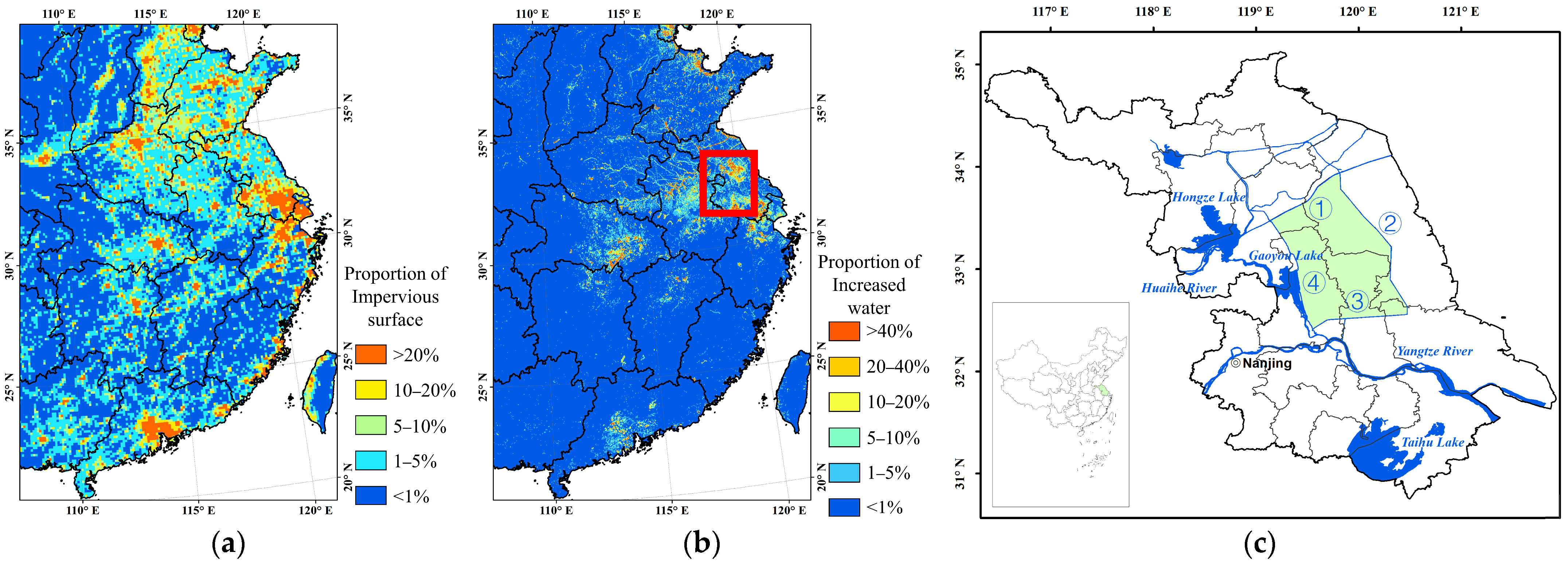
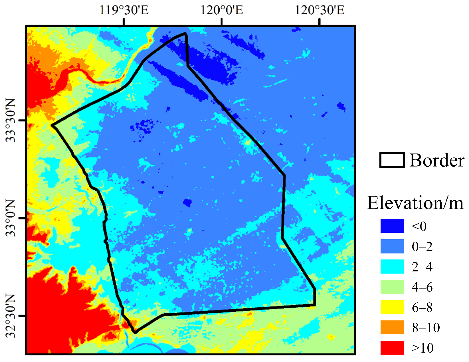
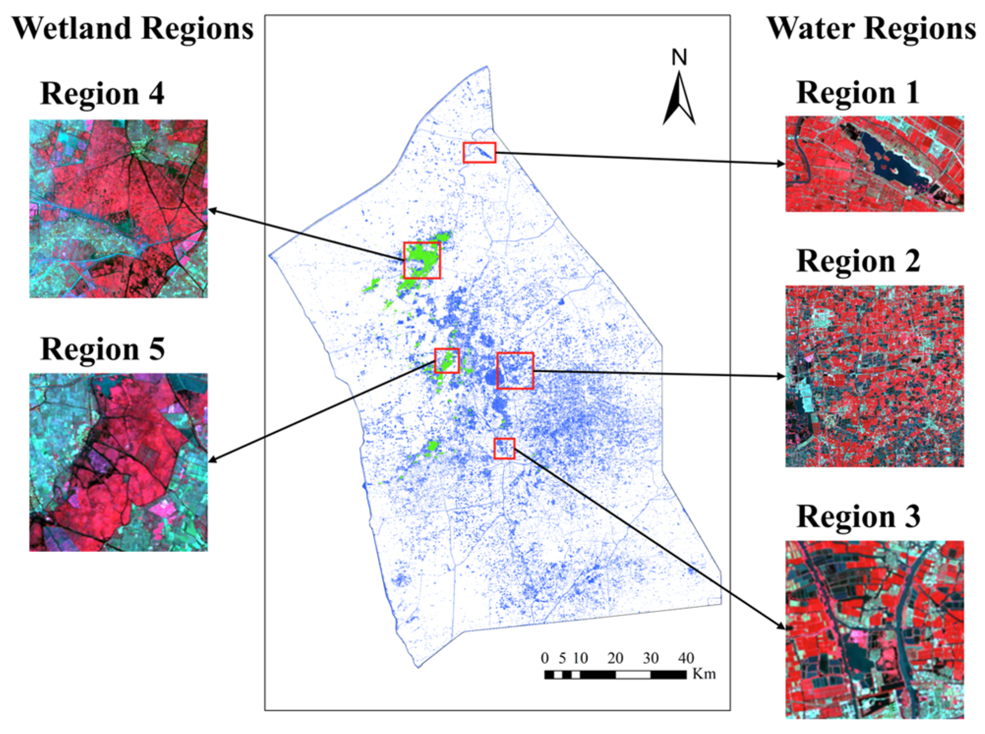
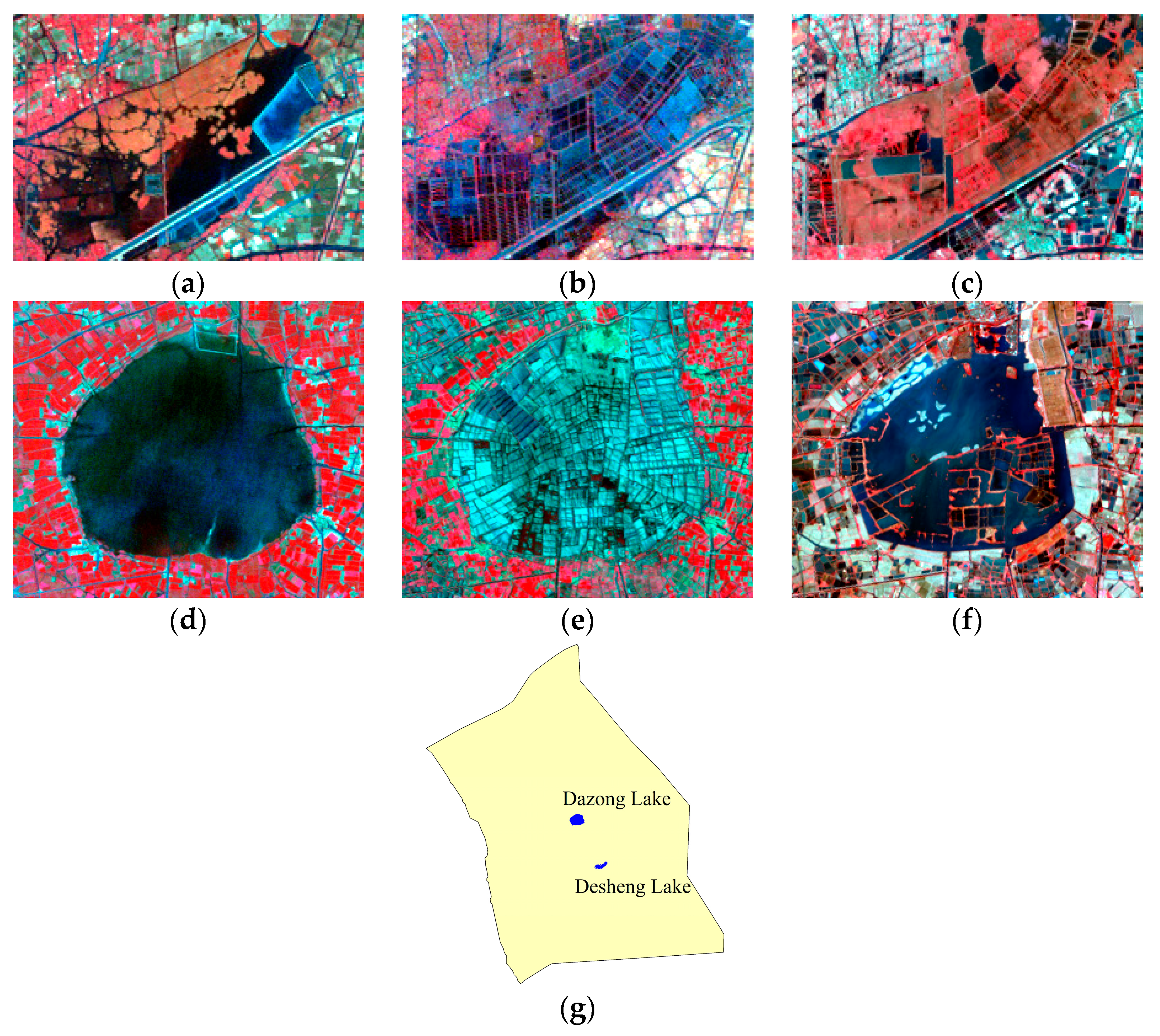
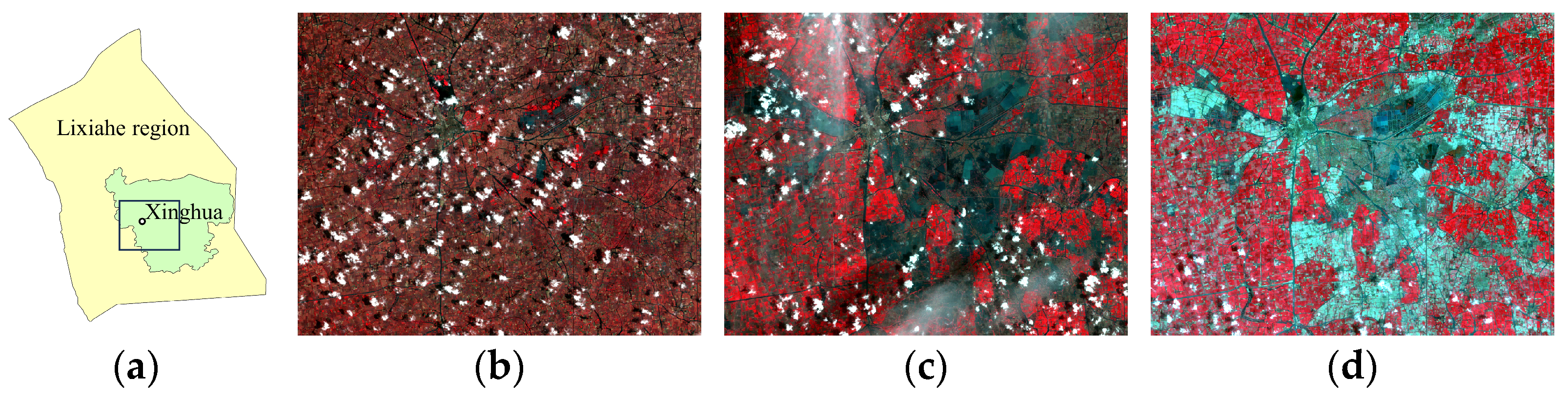
2.1. Study Area

The Lixiahe region, located in Jiangsu Province, is a flat area between the Yangtze River and Huaihe River with a dense network of rivers. It encompasses a vast territory to the south of the Main Irrigation Channel of North Jiangsu, west of Tongyu River, north of Tongyang Canal, and east of Li Canal, which is also a section of the Beijing–Hangzhou Canal, with a total area of approximately 11,571 km² (Figure 1c). Located in a subtropical monsoon climate zone, the annual average precipitation of this region is 1025 mm, with approximately 70% of the rainfall occurring during the flood season, which spans from June to September [42,43,44,45,46]. In terms of topography, the elevation range of the entire region is relatively low, typically ranging from 0 to 4 m above sea level, and the terrain at the periphery of the region generally exhibits higher elevations compared to the central areas (Figure 3).

The Lixiahe region’s topography, characterized by lower central terrain, creates a complex relationship between urbanization processes and changes in water area. On the one hand, areas with lower central terrain tend to form natural regions suitable for water resource storage, such as lakes, rivers, and wetlands. These water resources can be used for urban water supply, irrigation of farmland, and industrial purposes, providing a sustainable source of water for cities. On the other hand, in times of flooding, the lower central areas naturally take on the responsibility of flood control for the entire region. However, during the urbanization process, the flood storage capacity of the region is often easily compromised, leading to an increased risk of flood disasters. Due to a combination of climatic and topographic factors, the Lixiahe region constantly faces the threat of floods. Severe flooding events occurred in the Lixiahe region in 1991, 2003, 2006, and 2007, resulting in significant economic losses [42,43,44,47].

Due to population growth, numerous water conservancy projects were constructed in the Lixiahe area during the 1930s and 1940s, primarily for beach land reclamation purposes. In the 1960s and 1970s, guided by the policy that prioritized grain production, substantial efforts were invested in reclaiming lakes for agricultural purposes. Throughout the 1980s and 1990s, the exploitation of lakeside wetland resources was regarded as a means to achieve prosperity and affluence. The scope of development of lakeside wetland resources expanded from economically developed areas to those with weak economic foundations, resulting in a reduction of lakeside areas and storage capacity. Consequently, this expansion increased the vulnerability to flood disasters.

2.2. Classification System for Analyzing Water Resources and Urbanization

To analyze the relationship between water resources and urbanization, it is essential to establish a well-defined classification system.

Firstly, wetlands serve as vital reservoirs and sustainable sources of water resources, and play a pivotal role in controlling river runoff, replenishing groundwater, improving water quality, and maintaining the regional water cycle. Furthermore, changes in artificial impervious surfaces are a critical indicator for comprehending the impact of urbanization on both human society and the environment. These categories are the focus of our classification.

Based on the wetland classification systems proposed by Gong et al. [48] and Mao et al. [49], we have classified wetlands in the Lixiahe region into several subcategories, including lakes, rivers/canals, marshes, and aquaculture ponds. Among these subcategories, lakes, rivers/canals, and aquaculture ponds are water bodies. Therefore, we classified them as the ‘water’ category. This leaves only one remaining subcategory, marshes, within the wetland category (see

Table 1. Classification system used in this study, along with their false-color images.

Category	Subcategory	Description	Image Example
Wetland	Marsh	Natural wetland with dominant herbaceous vegetation.
Water	Lake	Natural polygon waterbody with standing water.
	River/canal	Linear waterbody with flowing water.
	Aquaculture pond	Polygon waterbody used for aquaculture with regular shape.
Impervious surface	-	Man-made structures that prevent natural infiltration of water into the soil.
Farmland	-	Cultivated areas dedicated to agricultural practices.

).

Excluding the mentioned categories, the remaining land is predominantly farmland, with small areas of bare land, water surface covered by aquatic plants, and public green spaces. Since these types do not align with the objectives of this study, they are all classified under farmland (see Table 1). When integrating classification results, we prioritize categories in a sequence similar to the decision tree method as follows: wetland > water > impervious surface > farmland.

2.3. Data Source

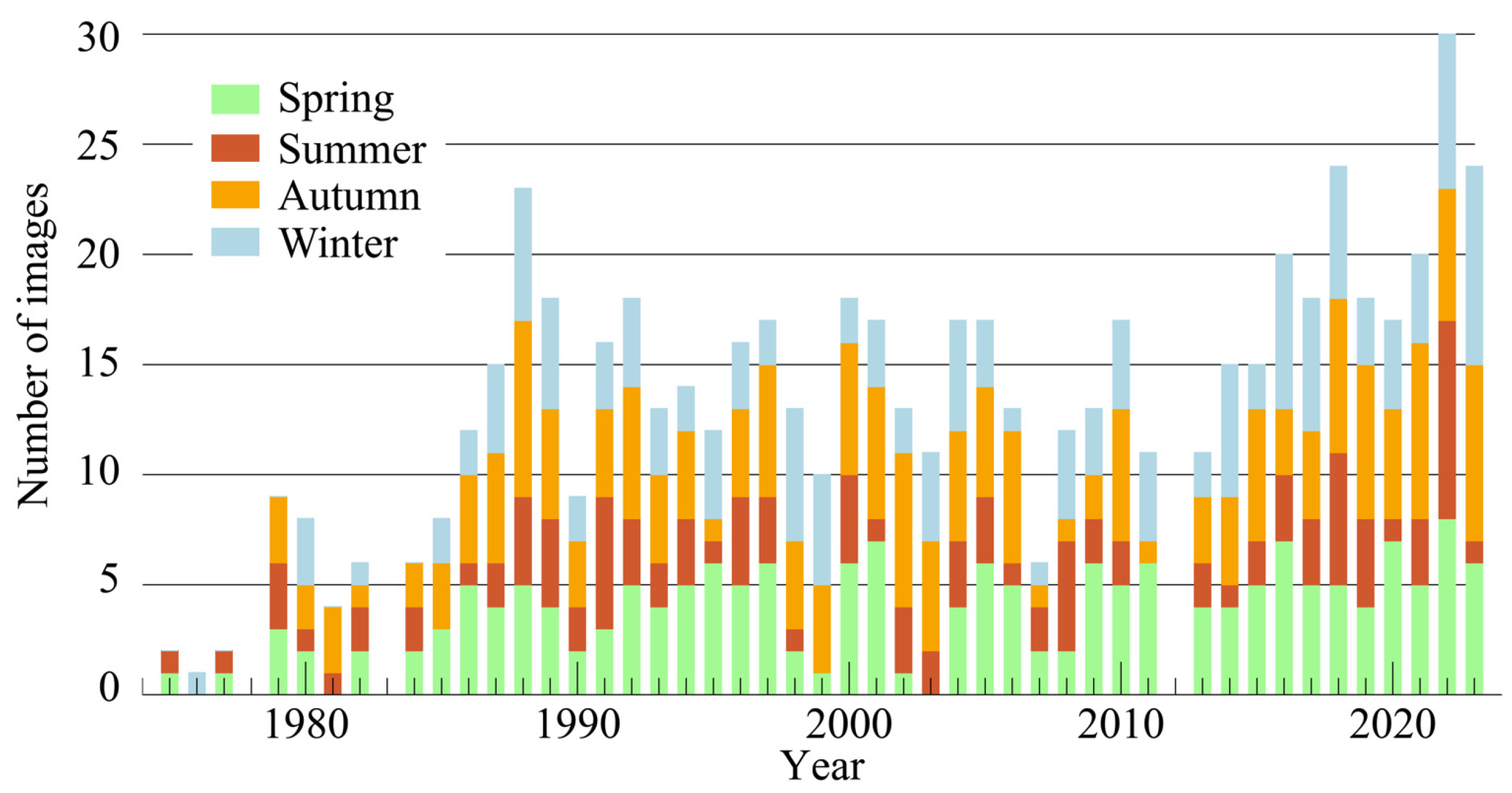
2.3.1. Satellite Imagery

The remote sensing images, including data from Landsat MSS, Landsat-5 TM, Landsat-8 OLI, and Landsat-9 OLI-2, are collected from the United States Geological Survey (USGS, https://earthexplorer.usgs.gov/, accessed on 4 January 2024). The spatial resolution of Landsat TM, OLI and OLI-2 images is 30 m. Landsat MSS images, on the other hand, originally have a 60 m spatial resolution, but for consistency with other Landsat data, they were resampled to 30 m. The stripe numbers (path/row) of the images covering this region are 120/037 and 119/037 in Landsat TM, OLI, and OLI-2, but 129/037 and 128/037 in Landsat MSS. In total, we selected 629 images with cloud cover below 20%, spanning the years from 1975 to 2023. The number of Landsat images for each season in each year is shown in Figure 4.

2.3.2. Digital Elevation Model (DEM)

DEM data play a crucial role in hydrological research, providing essential terrain information for the study area and enhancing our understanding of the distribution and dynamics of surface water. The Shuttle Radar Topography Mission (SRTM) [50] is an international project headed by the National Imagery and Mapping Agency within the United States Department of Defense and NASA. This mission covers land surfaces between 60 degrees north latitude and 56 degrees south latitude with a spatial resolution of 30 m. SRTM data have found extensive applications in various fields, including surveying, mapping, hydrology, meteorology, and military applications. The horizontal accuracy of the data is one arc-second, and it is expected that elevation measurements will have an absolute accuracy of less than 16 m. Similar to Landsat data, SRTM data can also be obtained from the USGS website (https://earthexplorer.usgs.gov/, accessed on 4 January 2024).

2.3.3. Impervious Surface Data

According to the classification system proposed in Table 1, the impervious surface is an essential category in this study. Over the past few years, researchers have produced several multitemporal global 30 m impervious surface products, including GAIA (Global Artificial Impervious Area) [51], GHSL (Global Human Settlement Layer) [52], GlobeLand30 impervious-surface layer [53], GISD30 (Global 30 m Impervious-Surface Dynamic dataset) [34] etc. We selected GAIA and GISD30 to acquire impervious surface data spanning from 1985 to 2020. We acquired the GAIA data for the years 1985 to 2018 from http://data.starcloud.pcl.ac.cn/zh/resource/13 (accessed on 8 October 2023) [51], and the GISD30 data covering the period from 1985 to 2020, accessible at https://doi.org/10.5281/zenodo.5220816 (accessed on 8 October 2023) [34]. Both datasets align with the study’s timeframe and were chosen for their accuracy and reliability.

GAIA’s results are available annually, whereas GISD30 supplies results every five years. We combined the results from these two products: a point in a year will be categorized as an impervious area if either of the two products for that year identifies it as such. In years when GISD30 does not provide results, as the formation of an impervious area is typically irreversible, we use data from the previous year directly. Due to the earliest available data for both of these products only goes up to the year 1985, we supplemented the data for the years 1975 to 1984 through visual interpretation.

2.3.4. Other Auxiliary Data

We also utilized the GSW data [37] and remote sensing images from satellite Gaofen-2 (GF-2). Furthermore, the gathering of economic, population, and other relevant data predominantly depends on the statistical yearbooks at the national and local levels in China [35,54], and data from the Food and Agriculture Organization (FAO) of the United Nations (https://www.fao.org/faostat/en/#data/FBS, accessed on 7 January 2024).

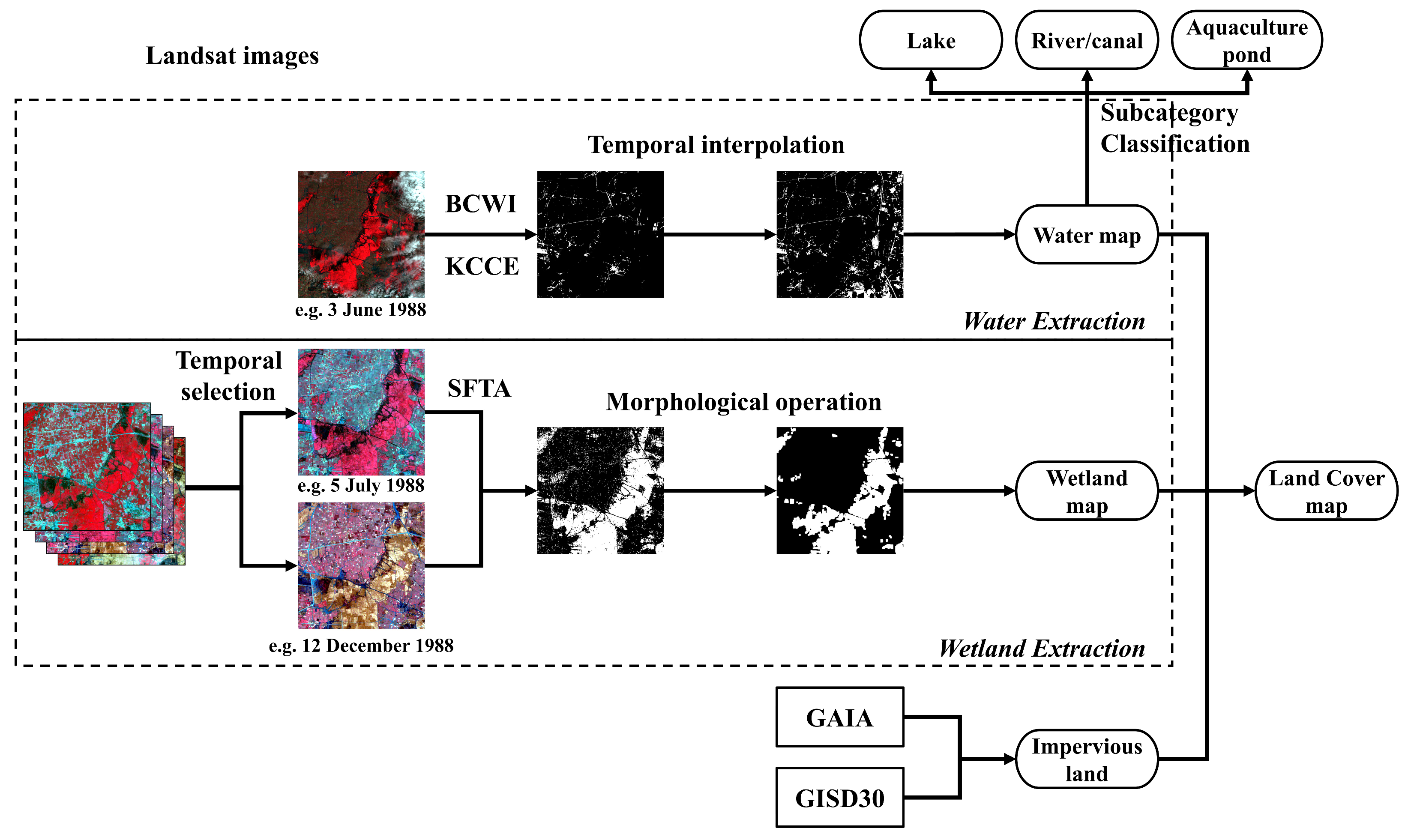
2.4. Method

The land cover mapping process in the Lixiahe region consists of two main components: (1) water extraction and (2) wetland extraction, as shown in Figure 5. The specific methods used, including KCCE (K-means Connection Center Evolution), BCWI (Band Compared Water Index), SFTA (Sum Filter Tensor Analysis), etc., will be introduced in detail in the following sections.

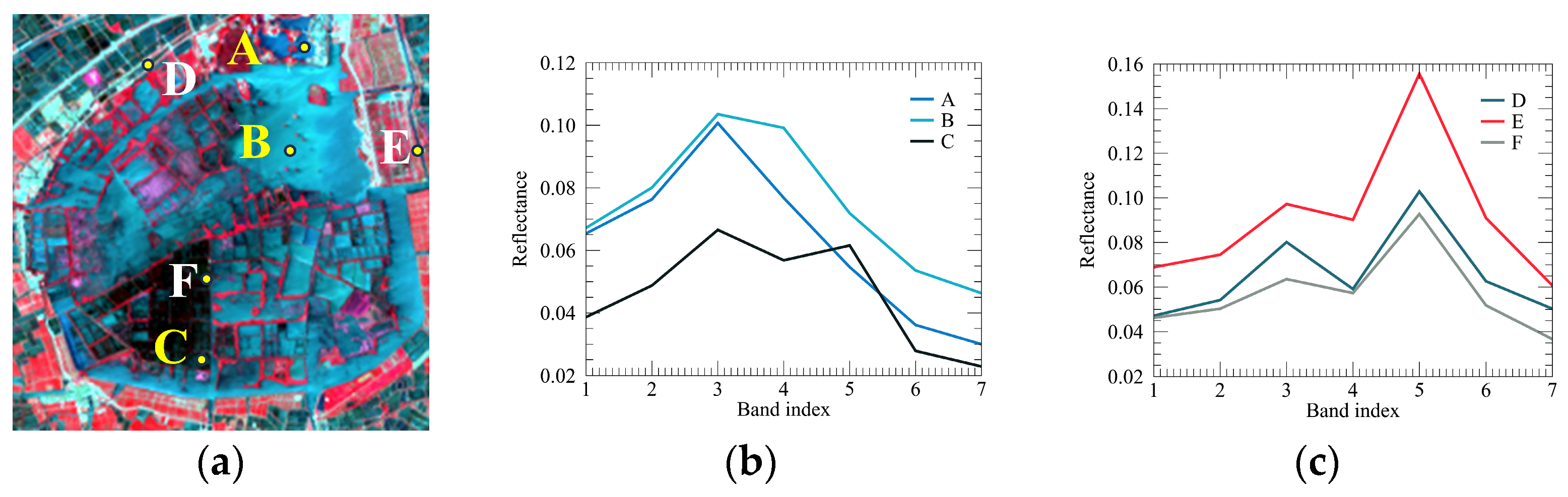
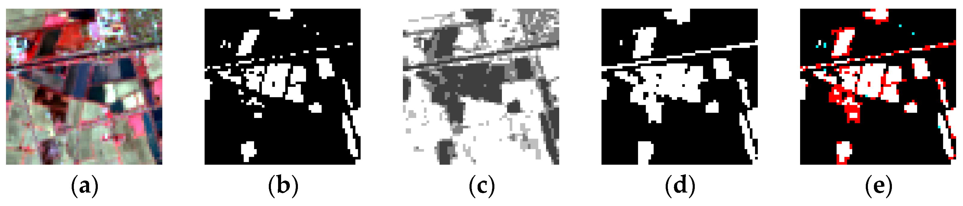
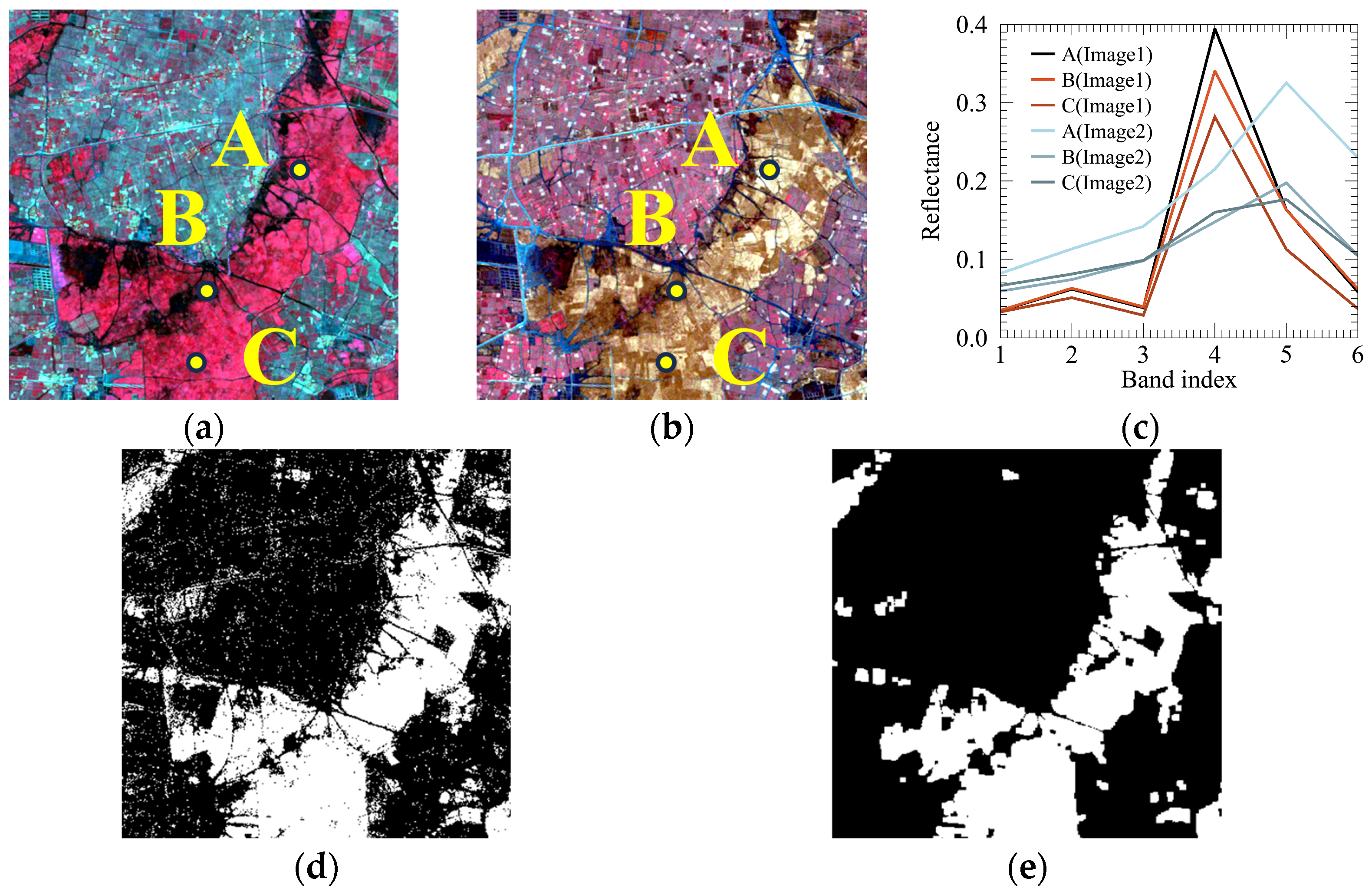
2.4.1. Water Extraction

Water extraction based on multispectral imagery can be roughly divided into two categories: pixel-based and object-based methods. The former is used to determine whether a pixel is water or not, while the latter focuses on identifying whether an entire object is water or not. The pixel-based approaches can be categorized into three classes: single-band thresholding, spectral indices and supervised classification. Generally, results for pixel-based methods often exhibit fragmentation [55,56,57,58,59]. On the other hand, the object-based methods take into account a range of factors such as the shape, size, texture, and spatial relationships of pixels within an object [60,61,62,63], so the results are more spatially compact.

In this study, we propose a combined method that integrates both approaches for accurate water body extraction. Firstly, we employ a spectral index method for pixel-wise water mapping. Subsequently, we utilize a clustering algorithm for object generation. Finally, we compute the water percent in each object and apply a thresholding technique to identify whether the object is water or not.

Pixel-Wise Water Extraction (BCWI)

In general, the reflectance characteristics of water exhibit higher reflectance in visible bands than in the shortwave infrared (SWIR) bands, as illustrated in Figure 6b. Therefore, we utilize the Band Compared Water Index (BCWI) [64] for pixel-wise water classification, which is

$$BCWI=\left\{\begin{array}{l}0, if\max \left({\rho }_{\mathrm{BLUE}},{\rho }_{\mathrm{GREEN}},{\rho }_{\mathrm{RED}}\right)\le \max \left({\rho }_{\mathrm{SWIR}1},{\rho }_{\mathrm{SWIR}2}\right)\\ 1, if\max \left({\rho }_{\mathrm{BLUE}},{\rho }_{\mathrm{GREEN}},{\rho }_{\mathrm{RED}}\right)>\max \left({\rho }_{\mathrm{SWIR}1},{\rho }_{\mathrm{SWIR}2}\right)\end{array}\right.$$

(1)

where ${\rho }_{\mathrm{BLUE}}$, ${\rho }_{\mathrm{GREEN}}$, ${\rho }_{\mathrm{RED}}$, ${\rho }_{\mathrm{SWIR}1}$, and ${\rho }_{\mathrm{SWIR}2}$ are the reflectance of blue, green, red and two SWIR bands of Landsat images. $BCWI=1$ for water pixels and $BCWI=0$ for non-water pixels. However, in our study area, emergent aquatic vegetation emerges in growing seasons. Due to the spectral mixing issue, the BCWI values for those mixed pixels remains at 1 (Figure 6c). To mitigate this misclassification, the Normalized Difference Vegetation Index (NDVI) is also applied here, which is

$$NDVI=\left({\rho }_{\mathrm{NIR}}-{\rho }_{\mathrm{RED}}\right)/\left({\rho }_{\mathrm{NIR}}+{\rho }_{\mathrm{RED}}\right)$$

(2)

where ${\rho }_{\mathrm{NIR}}$ is the reflectance of the Near Infrared (NIR) band of Landsat images.

Then a pixel is classified as water if it satisfies the following condition:

$$BCWI=1 and NDVI\le T_{\mathrm{NDVI}} and Cloud=0$$

(3)

where $T_{\mathrm{NDVI}}$ is the threshold for judging whether a pixel is vegetation based on NDVI. That is, when the NDVI is lower than this threshold, the pixel is considered not to be vegetation.

The Cloud flag is derived from the QA_PIXEL layer of the Landsat product. Here, $T_{\mathrm{NDVI}}=0.2$. For all Landsat images, we all use condition (3) for pixel-wise water mapping, as shown in Figure 7b.

Object Generation (KCCE)

In this study, we employ K-means Connection Center Evolution algorithm (KCCE) [65] for object generation. KCCE is an improved version of Connection Center Evolution (CCE), which can provide a set of dynamic clustering results and suggest a reasonable number of categories. However, CCE has a high computational complexity and requires a significant amount of memory to construct the similarity matrix, so it is not suitable on large-scale real remote sensing data [65]. By introducing the clustering results of K-means as input, KCCE can solve the above two issues and can be applied on large remote sensing imagery.

For KCCE, it has two parameters, the number of clusters for K-means, denoted $n_{\text{K-means}}$, and the final number of classes, denoted as $n_{\mathrm{CCE}}$. In this study, we set $n_{\text{K-means}}=100$ and $n_{\mathrm{CCE}}=5$. Generally, water pixels are generally clustered into one or two classes (Figure 7c). Then, each object is labeled with a unique ID for further processing.

Object-Wise Water Extraction (Combination of BCWI and KCCE)

For each object, we calculate the water proportion $p_{\mathrm{w}}$,

$$p_{\mathrm{w}}=N_{\mathrm{w}}/N$$

(4)

where $N_{\mathrm{w}}$ is the number of pixels classified as water by condition (3), and $N$ is the total number of pixels of that object. Then, an object will be classified as water if

$$p_{\mathrm{w}}\ge T_{\mathrm{w}}$$

(5)

In this study, we set $T_{\mathrm{w}}=0.6$.

As shown in Figure 7, it can be seen that the water mapping results of the BCWI are more fragmented, while the results of the object-based method are more spatial compact, especially for narrow rivers or channels.

Temporal Interpolation

Furthermore, due to the presence of cloud and cloud shadows, we also apply a temporal interpolation to the extraction of the water time series. Specifically, we first consider imagery no more than three months apart from the date of the missing data. This time window was set after reviewing the frequency and seasonal distribution of imagery available. When there are multiple suitable images available, we prioritize using the nearest neighboring image to fill in the missing data. If suitable images were not available within this timeframe, we then looked to images from the corresponding season of the previous or following year. In cases where this approach was still unsuccessful, other images from the same year were considered for gap-filling to compile a complete water time series.

Subcategory Classification

For further classification of water bodies, we distinguish between lakes, rivers/canals, and aquaculture ponds. Lakes and rivers/canals make up a minor fraction of the water objects, and their unique characteristics typically make them easy to discern. In the case of rivers, we utilized the findings from the national wetland mapping [39], and created a river mask. In the case of lakes, we manually identified any that had been converted into aquaculture ponds, which was necessary due to the development of many lakes for such purposes. Areas exhibiting features of aquaculture cages were classified as aquaculture ponds.

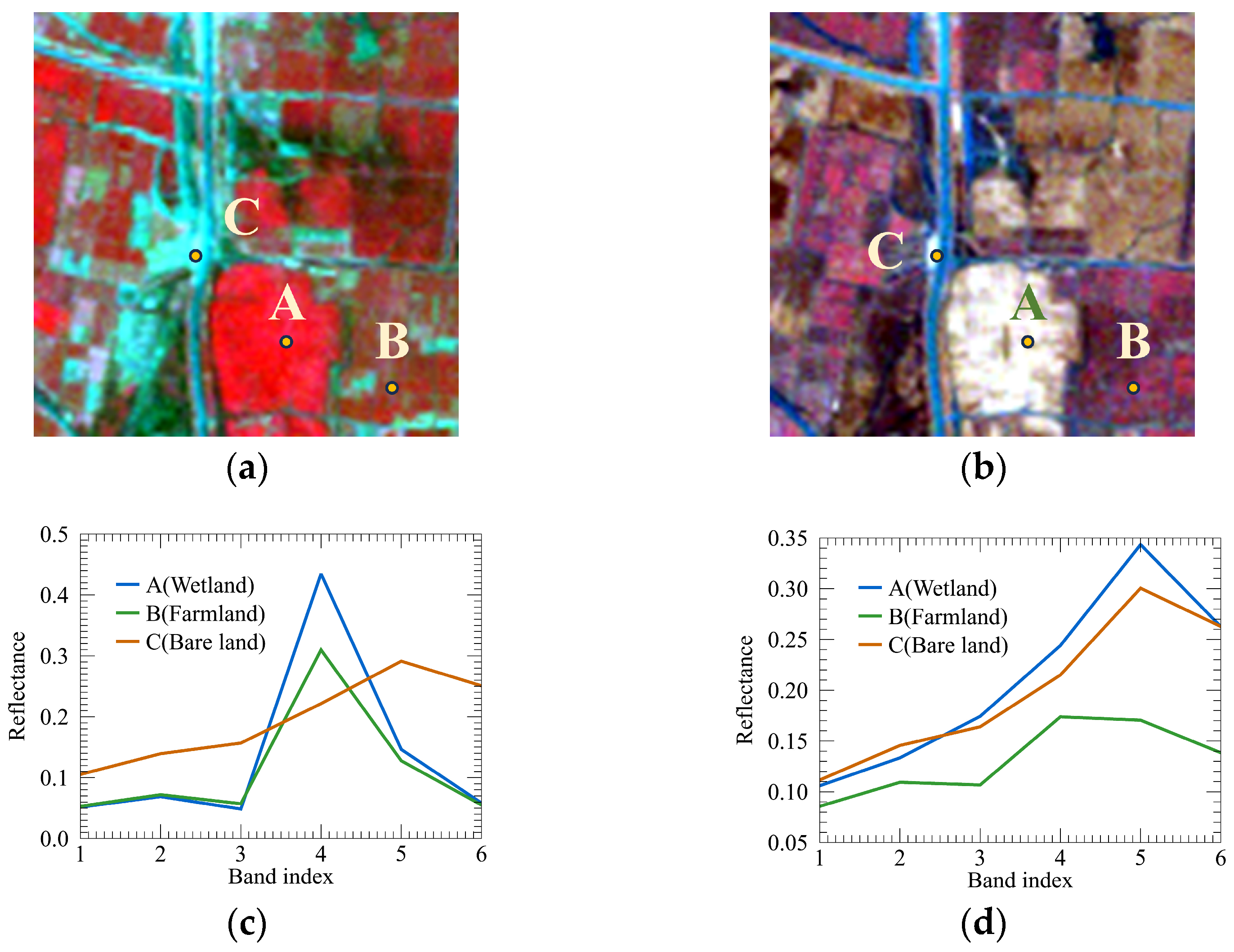
2.4.2. Wetland Extraction

Accurate mapping of wetland distribution is required to assess the impact of human activities on wetlands [66,67]. Different from water, wetlands lack specific spectral characteristics, and exhibit different spectral signatures in different seasons. In the study area, the vegetation growing season is approximately from April to October, while the non-growing season is roughly from November to March of the next year. Figure 8 presents two Landsat 5 images at 18 May 1988 (i.e., growing season) and 27 January 1988 (i.e., non-growing season), with a size 100 × 100 pixels, where Point A, B and C correspond to wetland, farmland, and bare land. We can see that in the growing season, the spectrum of the wetland pixel is similar to that of the farmland pixel, while in the non-growing season, the wetland’s spectrum is similar to the bare land’s.

As a result, using a single-phase image to detect wetland will lead to over-classification. Therefore, in this study, we will use multitemporal target detection method for wetland mapping, named Sum FTA (SFTA) [68]. The main steps of using SFTA for wetland mapping include: (1) time phases selection and (2) multi-temporal wetland mapping.

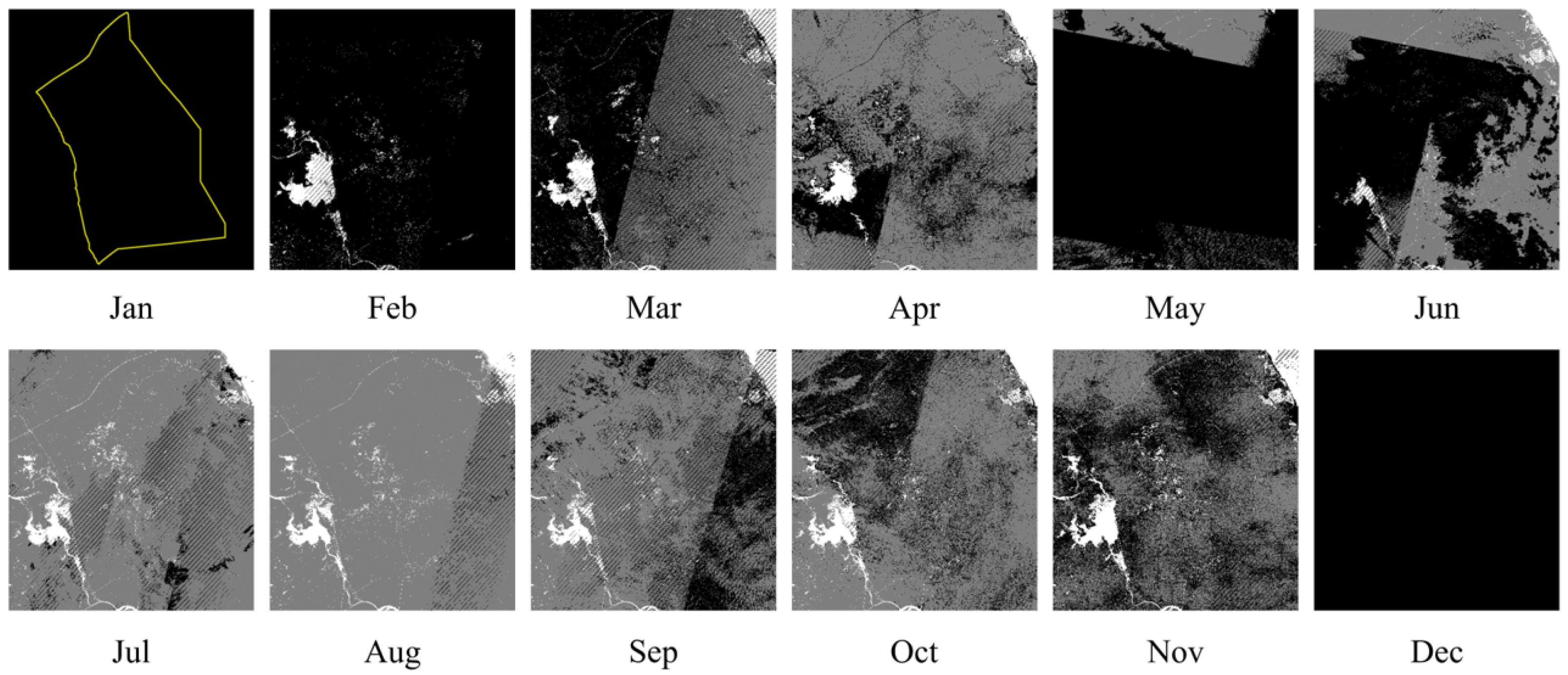
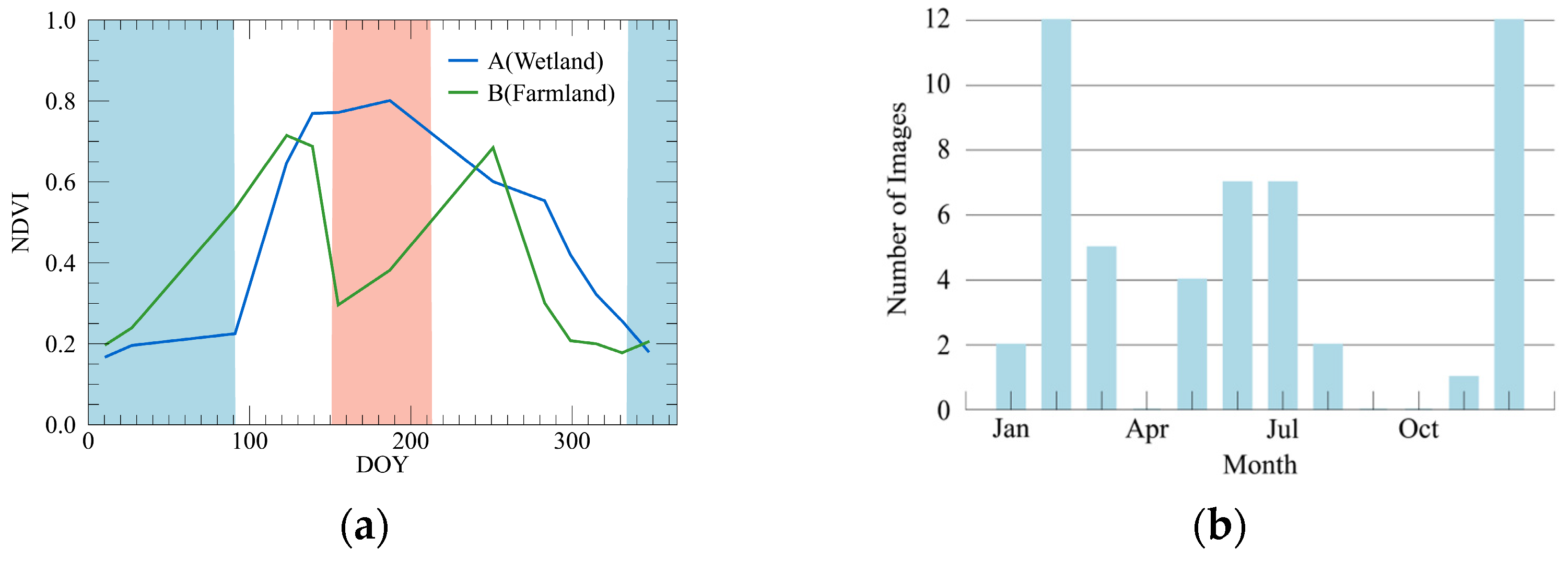
Temporal Selection

According to previous research, the target detection accuracy of the multi-phase method may decrease as the number of time phases increases [69], which is similar to the overfitting issue in machine learning [70]. According to Xi’s research, two time phases, which include one growing period and one non-growing period, can achieve the best performance for targets containing vegetation [69].

Figure 9a illustrates the annual variations of NDVI in 1988 for wetland and farmland pixels (corresponding to points A and B in Figure 8). It can be observed that the NDVI values for wetlands and farmlands differ significantly during the winter months (December to March) and the summer months (June to July), which belong to the non-growing and growing season, respectively. Therefore, each year, we firstly select two images for wetland mapping.

Figure 9b presents the monthly distribution of all the images used for wetland extraction. The acquisition time of images used each year are listed in

Table 2. The acquisition time of the two images used for wetland extraction each year. (Image1 corresponds to the image from the growing season, and Image2 corresponds to the image from the non-growing season. Dates with images from a non-corresponding season are bolded, and dates with images from neighboring years are underlined).

Year	Image1	Image2	Year	Image1	Image2
1975	7 June	5 December 1973	1989	22 June	14 February
1976	21 March	16 December	1990	11 July	18 December
1977	2 July	8 February	1991	28 June	4 February
1978	27 June	7 February 1979	1992	29 May	23 February
1979	13 June	7 February	1993	25 February	26 December
1980	22 July	2 February	1994	6 July	13 December
1981	17 July	4 December 1980	1995	22 May	30 January
1982	8 August	12 December	1996	2 February	18 December
1983	4 February	12 December 1982	1997	12 June	8 March
1984	27 August	18 January 1981	1998	30 May	24 December
1985	23 March	4 December	1999	1 May	27 December
1986	6 February	26 March	2000	22 July	16 March
1987	9 February	24 November	2005	2 June	26 February
1988	5 July	12 December

. When selecting images, our initial criterion is based on the months showing a significant difference in NDVI as depicted in Figure 9a. If no appropriate images are available during these months, we relax the criteria to any month within the growing or non-growing seasons. Image1 corresponds to the image from the growing season, and Image2 corresponds to the image from the non-growing season. Should this approach still prove unsuccessful, our last resort is to select two images from the non-growing season, marked in bold in the table, such as the year 1976, where the growing season’s Image1 was replaced with an image from 21 March due to the lack of suitable data. Moreover, if we cannot find two usable images within a year, we will choose images from neighboring years, marked with an underline. For example, the dates of the two images selected in 1978 are 27 June and 7 February 1979.

Multi-Temporal Wetland Extraction (SFTA)

After the temporal selection, we then use SFTA for annual wetland mapping. Due to the phenomenon of “the same object may have different spectra”, it is difficult to use one spectrum to represent all wetland pixels in the image. As shown in Figure 10, A, B, and C represent three wetland pixels, and their spectra vary from one another across different seasons. So, we suppose there are $q\left(q\ge 1\right)$ representative spectra for the wetland class, and let $FT{A}_j$ present the $j^{th}$ output of FTA detectors, then the SFTA detector is the sum of $q$ FTA outputs, which can be described as

$$SFTA\left(r_i\right)={\displaystyle \sum _{j=1}^{q}FT{A}_j\left(r_i\right)}$$

(6)

where $r_i$ is the reflectance spectrum of the $i^{th}$ pixel. The $j^{th}$ FTA detector can be solved by the following constrained optimization problem [71]:

$$\left\{\begin{array}{l}{\min }_{\mathcal{W}}\frac{1}{N}{\displaystyle \sum _i{\left(\mathcal{W}{\times }_1{r}_i^{(1)}{\times }_2{r}_i^{(2)}\cdots {\times }_M{r}_i^{(M)}\right)}^2}\hfill \\ \mathrm{s}.\mathrm{t}. \mathcal{W}{\times }_1{d}_j^{(1)}{\times }_2{d}_j^{(2)}\cdots {\times }_M{d}_j^{(M)}=1\hfill \end{array}\right.$$

(7)

where $N$ is the number of pixels, $M$ is the number of images, $\mathcal{W}$ is an $M^{th}$-order tensor filter, $d_j$ is the spectrum of the $j^{th}$ target pixel, and the operator ${\times }_k\left(k=1,2,\dots ,M\right)$ denotes the $k$-mode product operator.

In our approach, we select three 3 × 3-sized wetland targets each year, calculating the average spectrum of each target to obtain the target spectra. We then perform SFTA and set a threshold to obtain the wetland classification result. Due to the changing wetland range each year, different image acquisition times, and varying natural vegetation growth conditions, the target area selected for the algorithm differ every year. Figure 10 shows an example of wetland extraction using data from 1988, illustrating the overall process.

As shown in Figure 10a–d, using the multi-target and multi-temporal target detector can distinguish wetland from other land covers, including farmland and water.

Morphological Operation

However, the results appear to be quite fragmented, with many isolated small dots, resembling “salt noise” (see Figure 10d). These dots are primarily discrete patches of natural vegetation and are not part of the wetland. Therefore, we employ morphological operations (i.e., the opening operation, including the erosion and dilation of images) to eliminate these points, resulting in the improved outcome displayed in Figure 10e.

2.5. Accuracy Validation

To validate the accuracy of our land cover result, a total of 6600 samples are randomly selected and manually interpreted by experts. Five regions are selected as our validation areas. Among them, the first 3 regions (Region 1, 2 and 3) are selected to test the accuracy of our method on water extraction while the latter 2 regions (Region 4 and 5) are to validate the results of wetland, as shown in Figure 11. The primary water types of the first three regions are: Region 1—lakes and rivers, Region 2—lakes and aquaculture ponds, and Region 3—rivers and aquaculture ponds. A total of 3600 points are randomly collected on these 3 images. As for the two wetland regions, the majority land cover types are wetland, farmland, and river. A total of 3000 points are extracted from these images. Finally, the class type of each pixel is determined through visual interpretation and reference to Google Earth Engine by experts. Then, the Producer’s Accuracy (PA) and the User’s Accuracy (UA) are calculated for each class and, finally, the Overall Accuracy (OA) is computed [59,72,73].

3. Results

3.1. Accuracy of Water and Wetland Extraction

The confusion matrix of our results is presented in

Table 3. The accuracy of the land cover results of the Lixiahe region. Bold represents the overall accuracy.

	Land Cover Map Result
	Class	Water	Wetland	Impervious	Farmland	Sum	PA (%)
Visually interpreted samples	Water	1104	2	9	194	1309	84.34
	Wetland	0	1348	0	142	1490	90.47
	Impervious	0	0	190	0	190	100.00
	Farmland	71	56	35	3449	3611	95.21
	Sum	1175	1406	234	3785	6600
	UA (%)	93.96	95.87	81.20	91.12		92.29

. It can be observed that the UA for water body extraction is high (93.96%), whereas the PA is lower (84.34%). This indicates that although our water body classification results have a high level of accuracy, there are instances of underclassification, leading to an underestimation of water body areas. The misclassifications are predominantly associated with the “farmland” class, which can be attributed to the presence of numerous small-scale aquaculture ponds in the region. The water body extraction method faces challenges in accurately delineating mixed pixels at the water-land interface. Figure 12 illustrates a comparison between the manually interpreted results and the results extracted by our method from an area with small aquaculture ponds. In Figure 12b, the red dots represent points of underclassification, indicating that underclassification primarily occurs in mixed pixels along the water-land boundary.

In the extraction results of wetland, the UA is 95.87% and the PA is 90.47%, indicating a high level of accuracy in wetland extraction, and suggesting that the wetland extraction process is effective and reliable.

For impermeable layer results, the PA reaches 100%, but the UA is only 81.2%, suggesting a certain degree of underestimation in the GAIA and GISD30 products employed.

Overall, our mapping results demonstrate a high level of accuracy (with OA = 92.29%) and are deemed suitable for subsequent analyses.

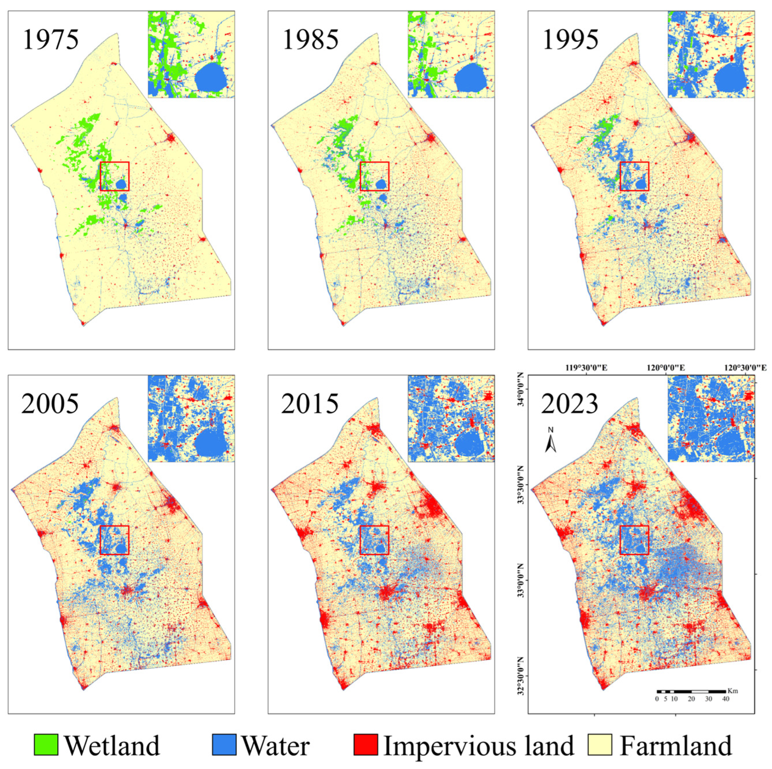
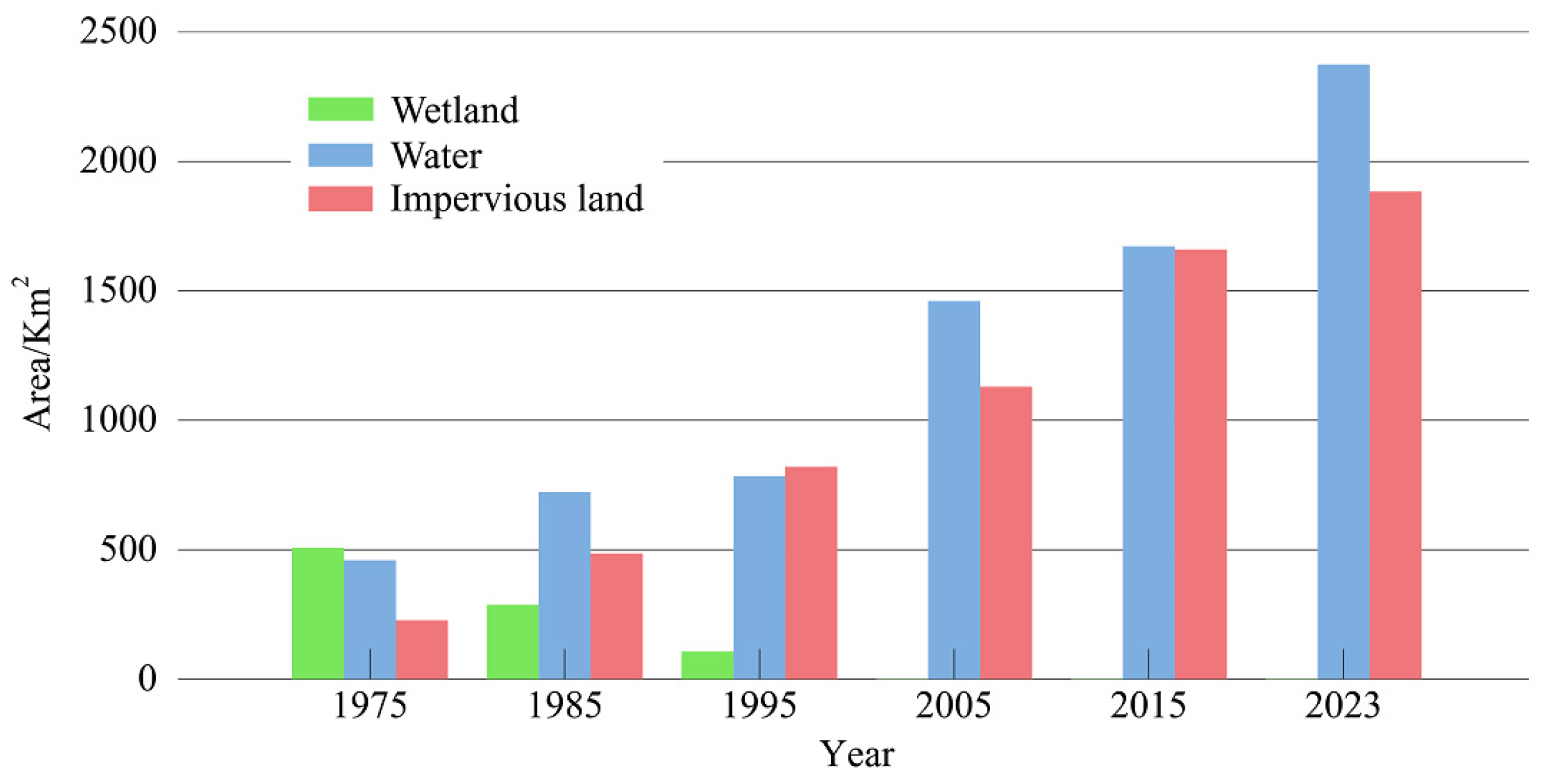
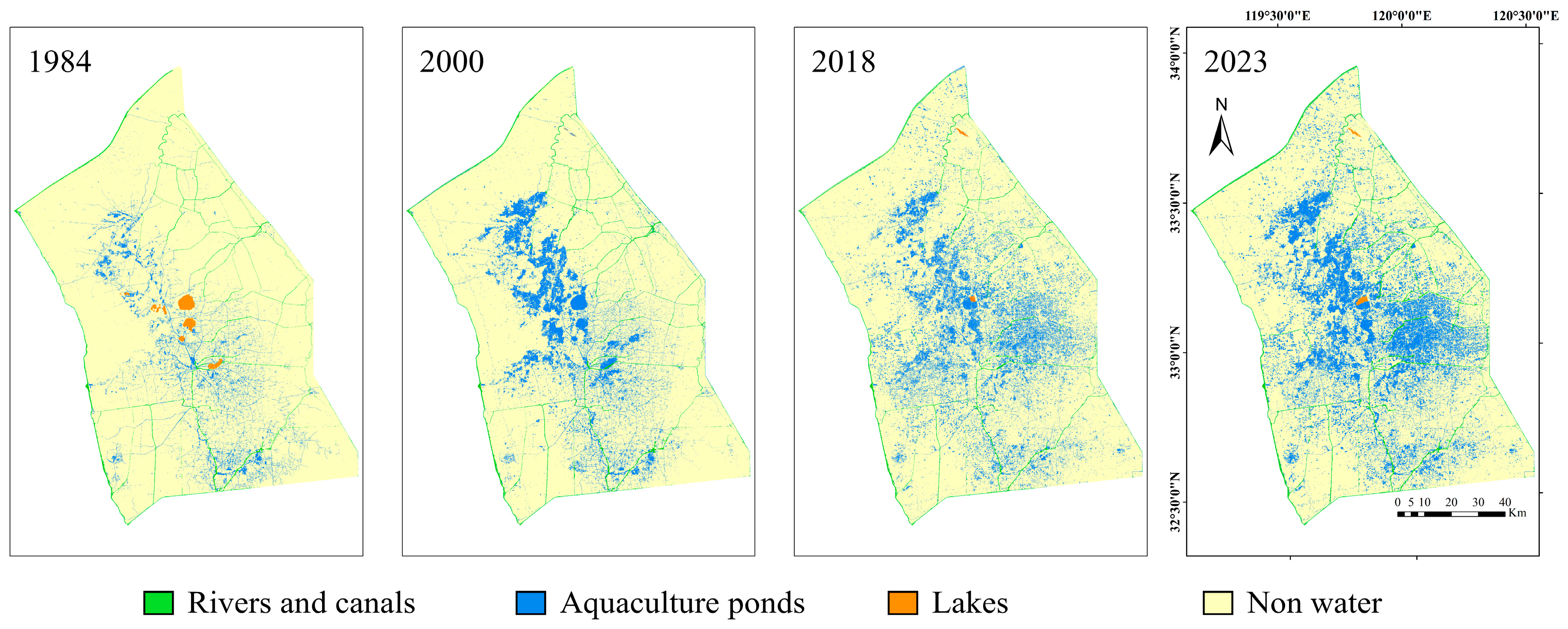
3.2. Changes of Land Cover Types in the Lixiahe Region since 1975

Figure 13 shows the changes of land cover types from 1975 to 2023, where an enlarged image of the area outlined by the red box in each image is provided in the upper right corner. We can see that wetland has suffered significant losses. In 1975, this region contained approximately 507.2 km² of natural wetland. However, after ten years, the area had decreased to 287.4 km² in 1985, with a decrease rate of 43.3%. Over the next 10 years, the decline was even faster, with a decrease rate reaching 62.9% in 1995, and the wetland area had decreased to 106.7 km² in 1995. By the year 2005, the wetland had almost disappeared. In contrast, the water area exhibited expansion, growing from approximately 459.3 km² in 1975 to 2373.1 km² in 2023. In addition, the impervious surface region also increased from 227.1 km² in 1975 to 1883.1 km² in 2023.

Figure 14 shows the changes in area for water, impervious surface, and wetland in 1975, 1985, 1995, 2005, 2015, and 2023. It can be seen that the wetland has almost decreased to 0 in 2005, while the water and impervious surface have gradually increased since 1975.

To better illustrate the transformation process of different land cover types in the Lixiahe region depicted in Figure 13, we selected 2005 as the central year and divided the entire period into two parts, 1975–2005 and 2005–2023, and calculated the total area of transitions between each type of land cover for both periods, and plotted a Sankey diagram, as presented in Figure 15.

The results indicate that during both stages, there were significant transitions from farmland to water and impervious land, with almost all impervious land originating from farmland. Wetland completely disappeared in the first stage and was mainly converted to water. However, in the second stage, some water was converted to farmland, but a greater amount of farmland was converted to water. Overall, by 2023, water bodies and impervious areas account for approximately 20.5% and 16.3% of the entire region, respectively. Urbanization has driven the expansion of impervious areas and the increase in water bodies, with most of the growth originating from former farmland.

3.3. The Transitioning Trend of Natural Wetland

In Figure 13, a noticeable reduction in the area of natural wetland is evident. Our current focus lies in comprehending the transition of wetland into other land cover types. Figure 16 illustrates the progression of this transformation within the Lixiahe region.

Natural wetland in this region underwent significant losses over the years. According to Figure 16, 1975–2023 can be divided into three stages.

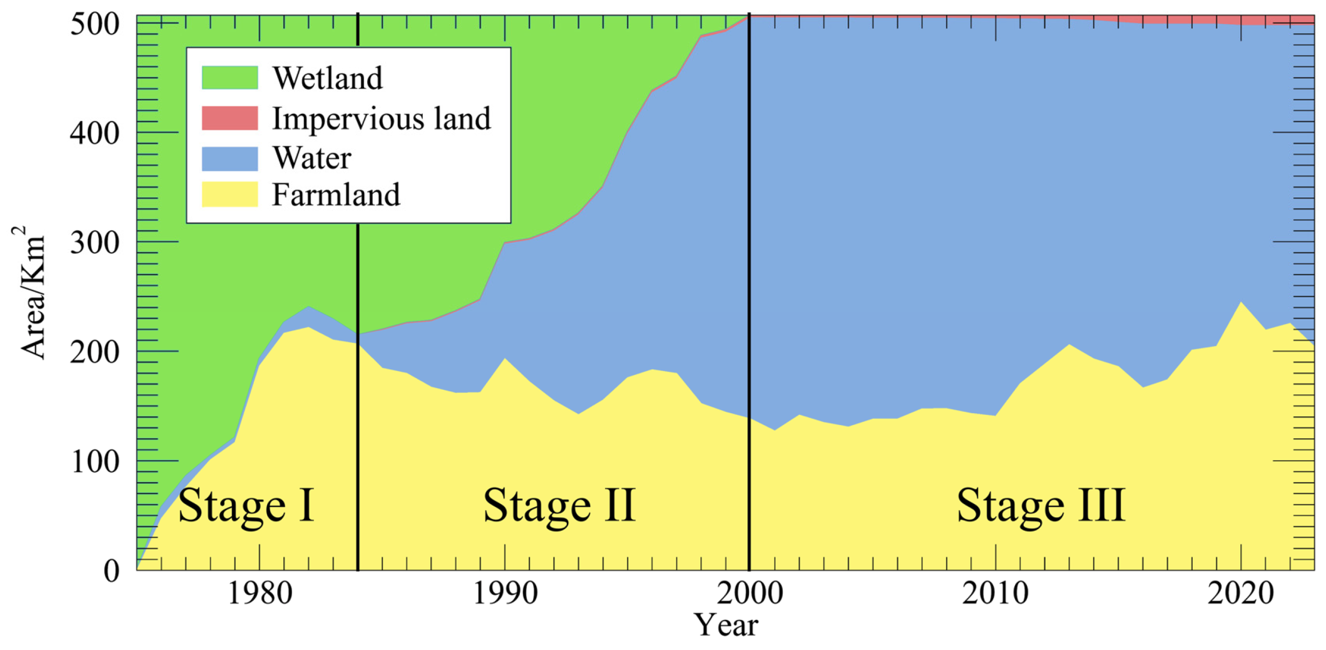
(1)

Stage I, 1975–1984, wetland to farmland. In this stage, a substantial portion of wetland converted into farmland.

(2)

Stage II, 1984–2000, wetland to water. In this stage, the extent of farmland conversion remained relatively stable, while most of the wetland transitioned into water bodies. This transition could be attributed to governmental policies that promoted industrial expansion, a topic we will discuss later, combined with societal realities.

(3)

Stage III, 2000–2023, absence of wetland. Around 2000, virtually all wetlands had vanished, and this marked the beginning of a new stage. In these years, part of the water bodies became farmland.

Notably, the proportion of areas transformed into impervious surfaces accounted for merely about 1.8%, significantly lower than the average of the entire region’s 16.3%. This might be related to the soil conditions of the wetland.

In conclusion, the transition of natural wetland into other land cover types is a significant trend in the Lixiahe region. Our analysis points to a shift from wetland to farmland, followed by a transition to water bodies. The lower rate of impervious surface development might be linked to soil conditions. This information is crucial for understanding land cover changes and their implications for the region’s environment and land use policies.

3.4. The Transitioning Trend of Water Bodies

Due to the low resolution and the lack of available images from Landsat MSS, for each year from 1975 to 1983, we only obtained one water area result for each year from 1975 to 1983. Starting from 1984 with Landsat 5, 8, and 9 images, which offer higher-quality data with improved resolution, we produced a box plot, as shown in Figure 17, to illustrate the change in water area in the entire Lixiahe region since 1984. Owing to the dynamic nature of water bodies and variations in image acquisition dates and cloud cover conditions, it is necessary to establish a criterion to determine the water area for each year.

Figure 17 presents the dynamic changes of water bodies in the Lixiahe region from 1975 to 2023 using a box plot. It should be noted that for each year from 1975 to 1983, we only obtained one water area result from Landsat MSS data. In addition, no usable images were acquired for the years 1978 and 1983, and as such, no water body extraction results are provided for these years. Starting from 1984, imagery from Landsat 5, 8, and 9 offered finer resolution and lower time interval data, allowing us to present box plots that illustrate the variations in the water body area of the entire Lixiahe region.

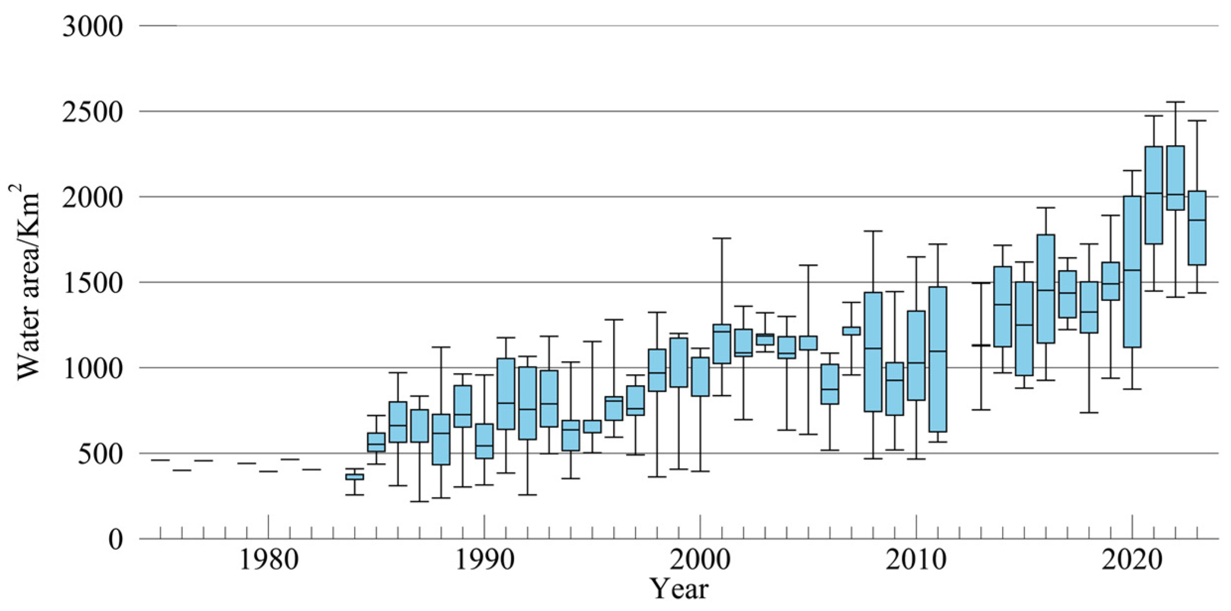
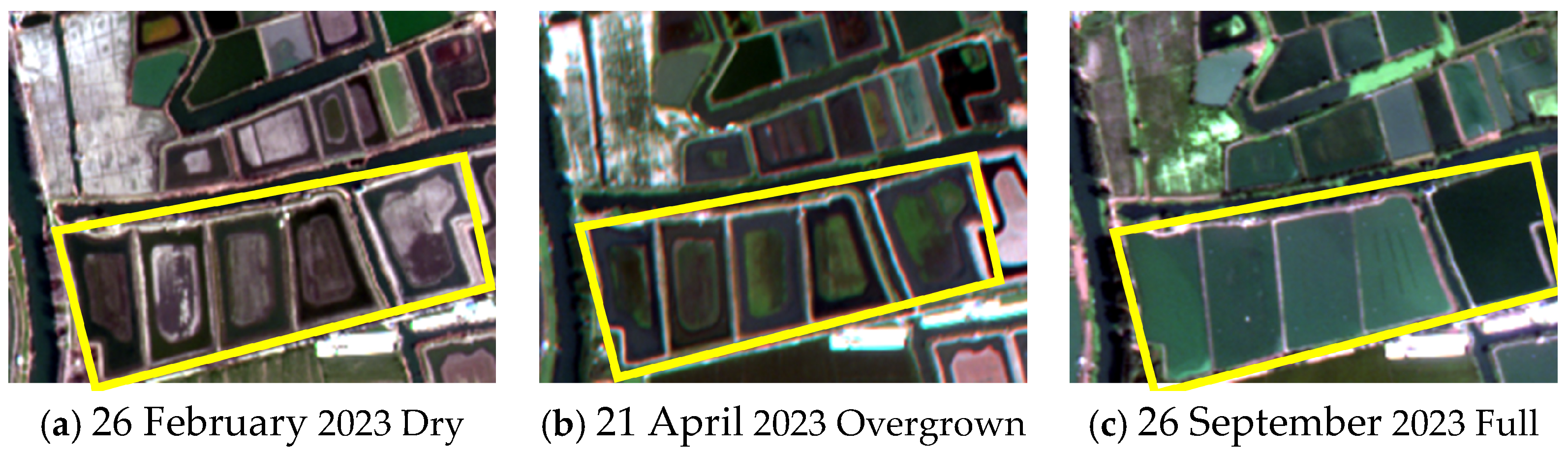
3.4.1. Intra-Annual Variation of Water

Figure 17 illustrates that within a single year, there is a considerable range of variability in the water bodies of the study area. Results of water body extraction during different periods within a year may vary due to the impact of aquatic vegetation growth and the dry pond period, as shown in Figure 18. Therefore, it is essential to establish a standard for determining the annual water surface area accurately.

To determine water bodies for each year, we face challenges: the drainage periods of ponds in different areas of the Lixiahe region are not consistent, and the presence of aquatic vegetation on the surface of ponds also affects the determination of water bodies. This makes it difficult to use a single image to determine the distribution of water bodies in a given year. To address this problem, we established a criterion: considering N available images in a given year, if water is detected in no fewer than N/3 images, the pixel is classified as water for that specific year. Based on this criterion, we calculated the annual water area, which is shown in Figure 19.

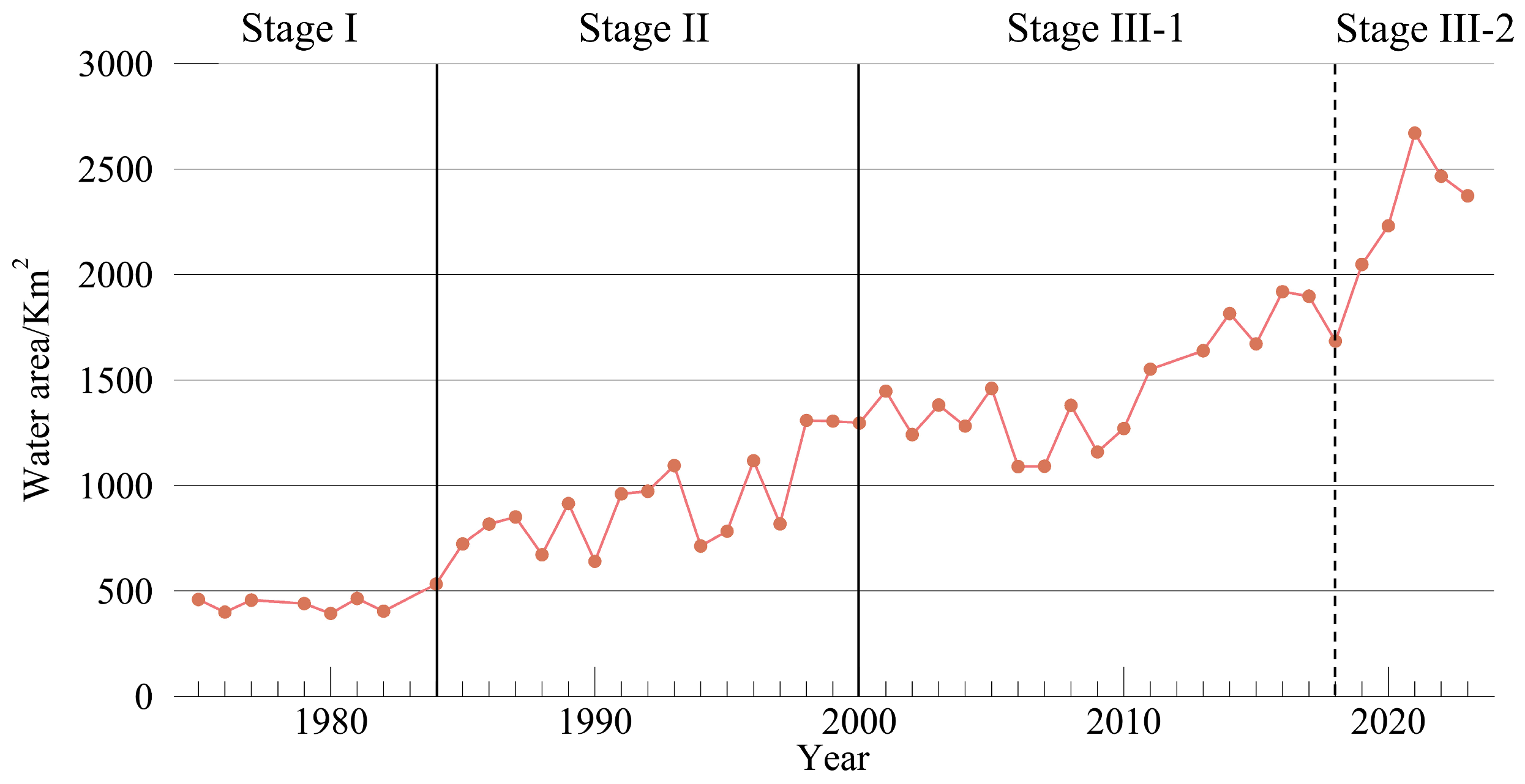
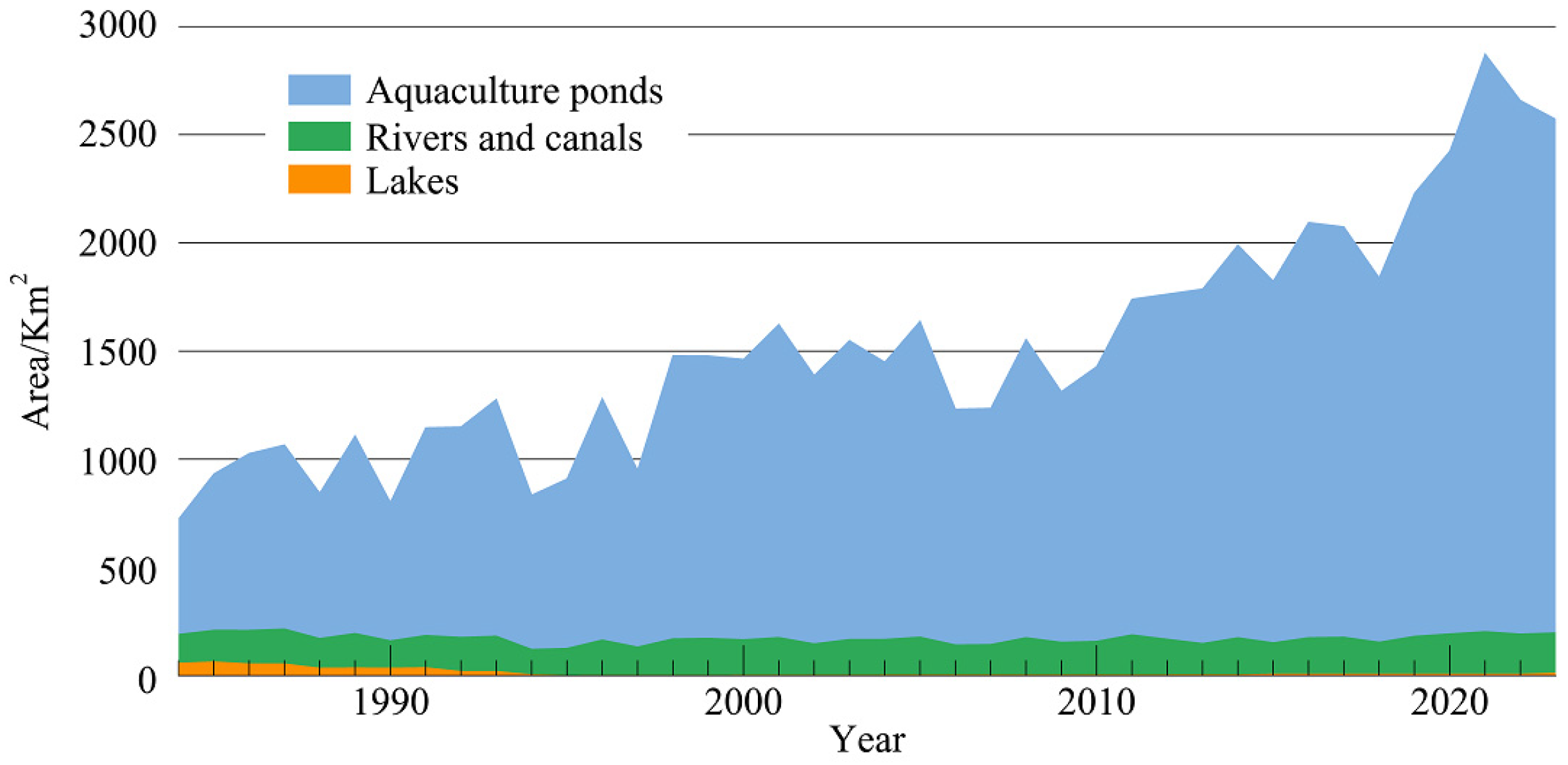
3.4.2. Interannual Variation of Water

According to the water area in Figure 19 and the stage division from Figure 16, we categorized the period from 1975 to 2023 into four stages: Stage I: 1975–1984; Stage II: 1984–2000; Stage III-1: 2000–2018; Stage III-2: 2018–2023. In Stage I, there was no significant trend in water surface area; in Stage II, there was a rapid increase in total water area; in Stage III-1, the water area increased slightly; and in Stage III-2, there was a marked resurgence in water area growth. To gain a clearer understanding of the spatial distribution of water changes within these stages, we conducted a statistical analysis of areas where water increased and decreased during Stages II, III-1, and III-2, as shown in Figure 20.

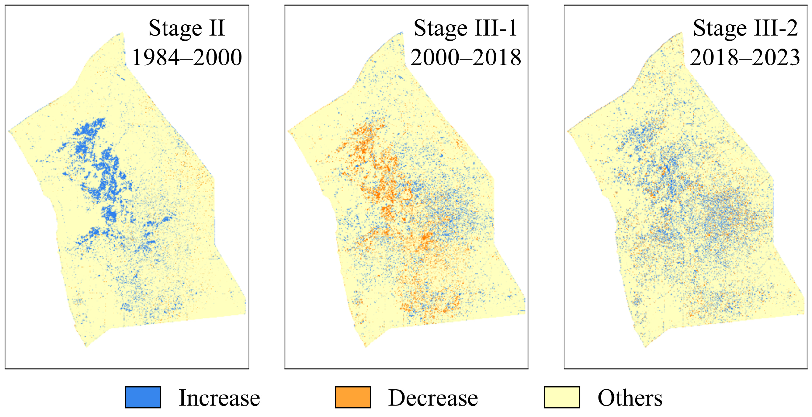
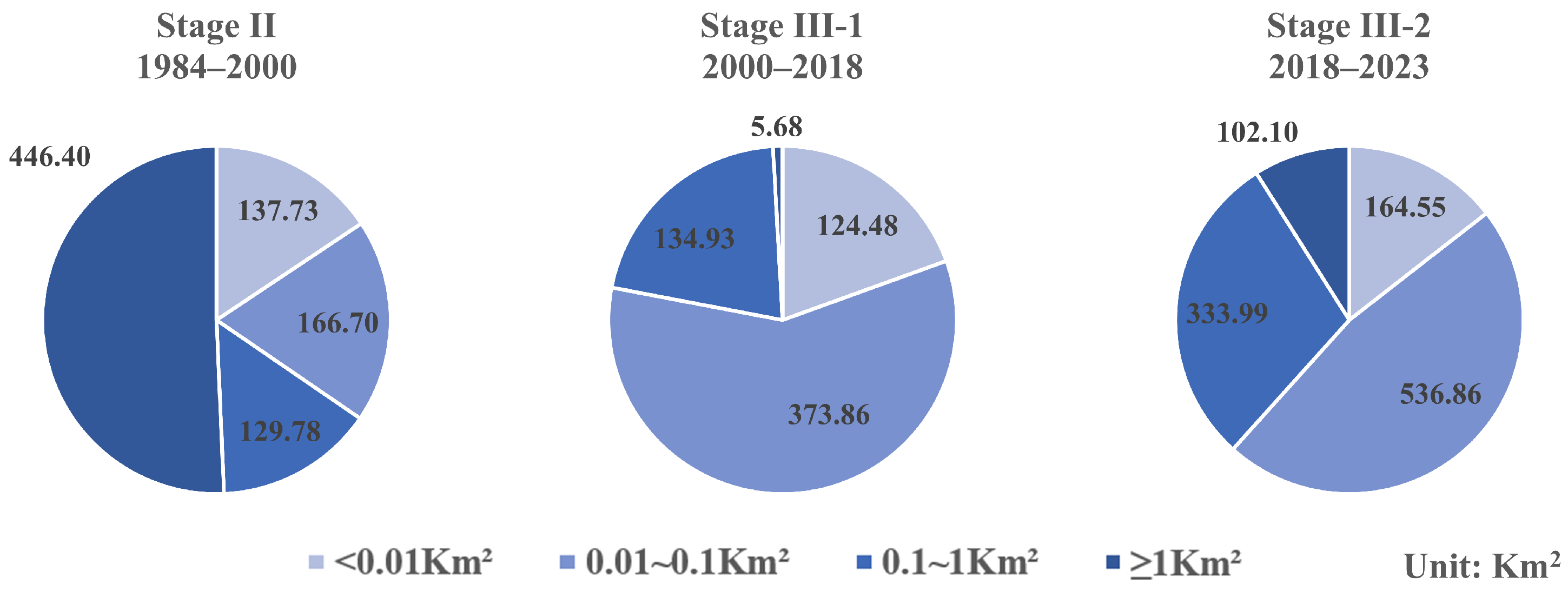
(1)

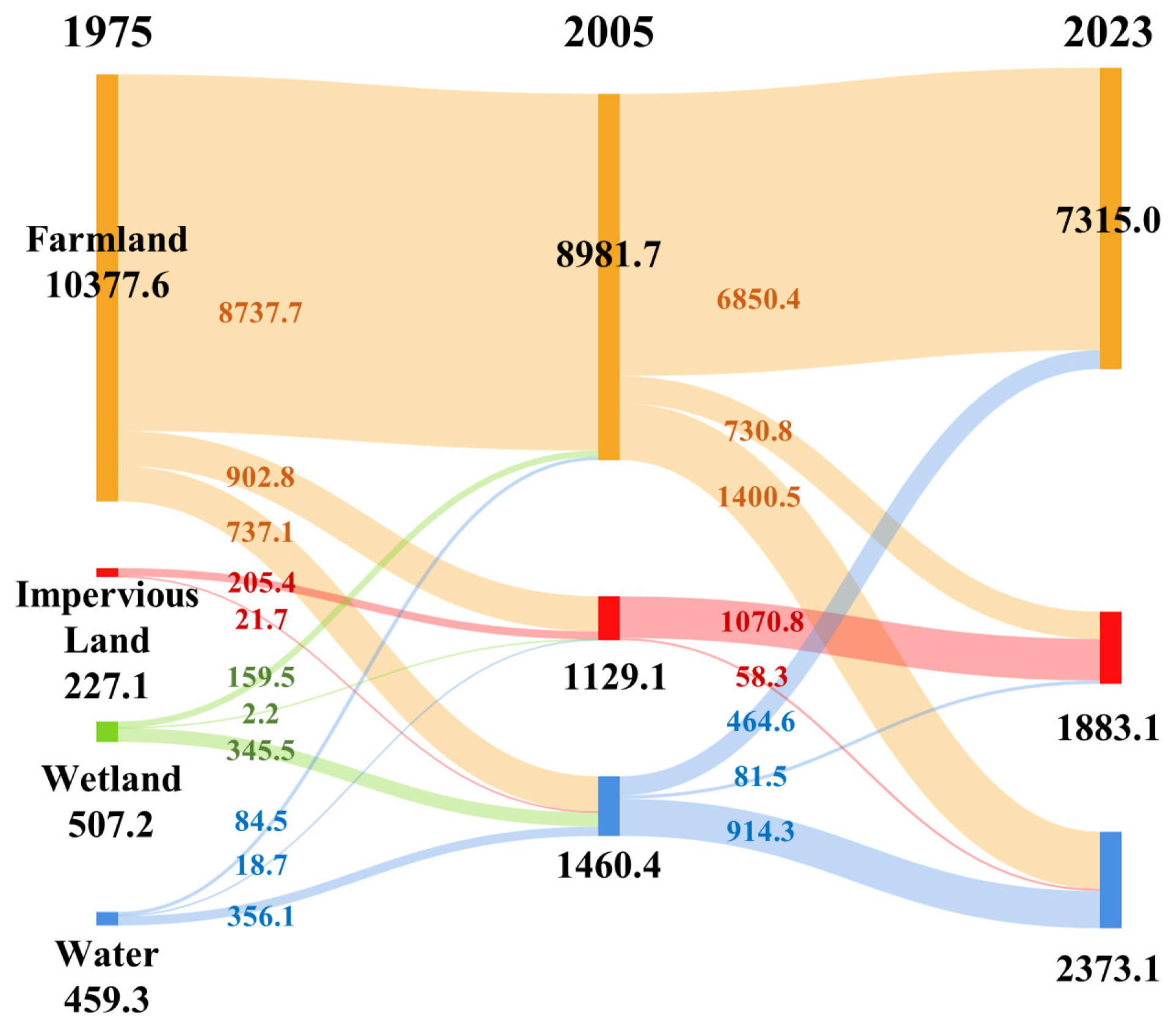
In Stage II, the increase in water bodies primarily originated from areas that were wetlands in the early stages. This trend is also reflected in Figure 16.

(2)

In Stage III-1, the rate of increase in water bodies slowed down. During this period, many water bodies transitioned to non-water bodies. These areas were predominantly those that had transformed from wetlands to water bodies in the previous stage. The newly formed water bodies were mainly fragmented and small, consisting mostly of ponds.

(3)

In Stage III-2, the growth in water bodies was also predominantly in the form of aquaculture ponds. The increased water bodies during this period were also mainly concentrated in the eastern area, coinciding with the main growth areas in the previous stage.

For the newly emerged water during the three periods shown in Figure 20, we separately calculated the total area of water bodies of different sizes, as illustrated in Figure 21. It can be observed that during the period 1984–2000, the increased water bodies show higher connectivity, with nearly half of the total newly added water area being water bodies larger than 1 km². In the subsequent two periods, water bodies smaller than 0.1 km² accounted for more than two-thirds of the total newly emerged water area, while water bodies exceeding 1 km² constituted only a minimal proportion. Upon evaluation, these newly emerged water bodies are principally utilized for aquaculture. This observation suggests that the differences noted may be correlated with the types of original land cover that have been transitioned to aqueous environments.

During 1984–2000, the majority of increased water bodies originated from wetlands. The natural hydrological similarities between wetlands and aquaculture ponds were key factors contributing to the higher connectivity in these regions. Wetlands, characterized by abundant water resources and lower land elevation, facilitated the drainage and retention of water when transformed into aquaculture ponds. Additionally, wetlands typically exhibit contiguous distribution, a geographical characteristic that tends to form interconnected networks of aquaculture ponds, thereby enhancing overall regional connectivity.

In contrast, after the year 2000, the growth of water bodies primarily originated from farmlands. Farmlands are often situated at higher elevations or areas with superior drainage conditions compared to wetlands. Consequently, transforming these areas into aquaculture ponds requires substantial land leveling and water management measures, naturally resulting in lower overall connectivity compared to the transformation of wetlands into aquaculture ponds.

3.4.3. Variation of Different Water Subcategories

In addition to the overall changes in water bodies, we conducted a detailed analysis of the changing trends in different subcategories of water within the study area. As outlined in Table 1, we devised a classification system that categorizes the water bodies into three subcategories: lakes, rivers and canals, and aquaculture ponds. The specific classification method is introduced in Section “Object-Wise Water Extraction (Combination of BCWI and KCCE)”.

We illustrated the distribution of various subcategories of water during key transition years outlined above, specifically 1984, 2000, 2018, and the most recent year, 2023, as depicted in Figure 22. Corresponding changes in area from 1984 to 2023 are presented in Figure 23. Our findings reveal a concerning trend where many lakes are being repurposed for aquaculture, resulting in significant losses for the natural lake ecosystems. In contrast to lakes, the overall area occupied by rivers in the region has not exhibited significant changes. These observations allow us to infer that the rapid expansion of water areas can primarily be attributed to the increasing prevalence of aquaculture ponds.

4. Discussion

4.1. Factors Influencing Water and Wetland Changes in the Lixiahe Region

The transformation of the Lixiahe wetland and water ecosystems is a complex process influenced by multiple factors, mainly including population dynamics, economic developments, demand growth, and policy interventions.

4.1.1. Stage I: Wetland Reclamation

During the period from the 1950s to the 1970s, China experienced a rapid population growth. By the year 1980, the population had reached 987 million, which was 1.8 times the population of 542 million in 1949. Simultaneously, China embarked on a vigorous path of industrialization, leading to a substantial rise in urban population and an increased demand for food resources. To bridge the food supply gap, the Central Committee of the Communist Party of China (CPC) introduced policies prioritizing grain production and comprehensive development. These policies, in turn, triggered extensive wetland reclamation, including marshes and lakes, to convert them into farmland. This corresponds to the result in Figure 16, which shows that wetland was extensively reclaimed as farmland before the 1980s.

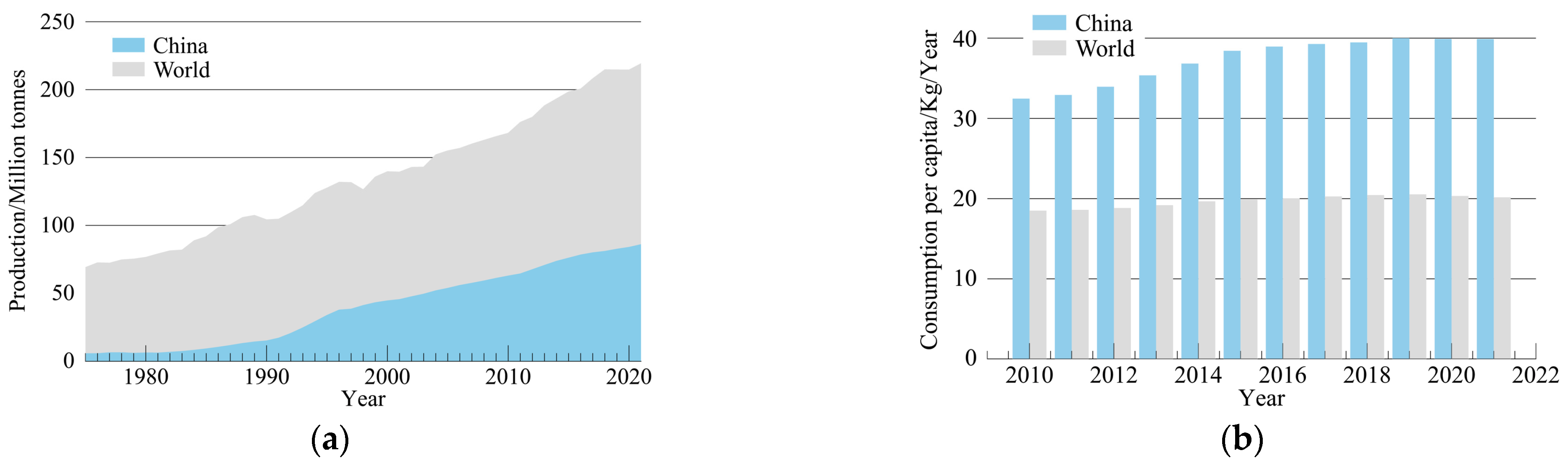
4.1.2. Stage II and III: Aquaculture Thriving

With the growth of the population and the development of the Chinese economy, people’s income levels have risen, leading to changes in dietary patterns and an increased demand for high-quality, diverse aquatic products. To meet this growing demand, a legal framework for the conservation and management of fisheries resources was gradually established in China in the mid to late 1980s. In 1985, the CPC Central Committee and the State Council issued the “Directive on Relaxing Policies to Accelerate the Development of Aquaculture”, strategically accelerating the development of aquaculture, adjusting the rural industrial structure, and promoting agricultural transformation. Subsequently, in 1986, the “Fisheries Law of the People’s Republic of China” was promulgated. The issuance of these policies had a profound impact on China’s aquaculture industry. Figure 24 depicts the changing trends in aquatic food production quantity of China and the world from 1975 to 2021, as well as the trends in consumption per capita per year from 2010 to 2021, sourced from FAO [74].

In 2021, China’s aquatic food consumption accounted for over one-third of the global total, with a per capita annual consumption reaching 39.89 kg, nearly twice the world average of 20.16 kg. As the world’s largest producer and consumer of aquatic products, China plays a pivotal role in shaping the global aquatic food supply chain. This is linked to China’s robust aquaculture sector, which has been heavily emphasized through government policies and technological advancements in recent years.

Based on our results, in Figure 17, the overall water area remained basically unchanged before 1984, but then increased significantly. Moreover, Figure 16 shows that after 1984, the reduced wetland mainly changed into water bodies. These are the results of the expansion of the aquaculture industry under policy guidance.

The increase in agricultural and aquacultural land promotes regional economic development, but it has also raised the hazard of flooding. The shrinkage of wetland impairs their regulation and storage capacity. Furthermore, the expansion of artificial impervious areas, driven by industrialization and urbanization, reduces the waterlogging drainage capacity.

4.1.3. Stage III: Ecological Protection Strengthening

After the devastating Yangtze flood of 1998, the Returning Farmland to Lake Program was established to encourage the conversion of farmland into natural lakes, with the primary focus on restoring the flood retention capacity of lakes. Since the beginning of the 21st century, the Jiangsu Provincial People’s Government and the Department of Water Resources of Jiangsu Province have issued various documents, including lake protection regulations and specialized plans for reintegrating dikes with lakes. These documents underscore the significance of improving lake management and protection measures, with a specific focus on restoring dike systems to fortify lake embankments and ensure flood control safety. Furthermore, they aim to enhance ecological preservation, boost the environmental capacity of lakes, and elevate water quality standards.

Under the guidance of policies, a significant portion of farmland has been transformed into water bodies. However, the satellite imagery and the results presented in Figure 22 indicate that the areas transformed into water bodies are mostly utilized for aquaculture, with limited presence of natural water surface. By 2023, some lake areas have been restored to free water surfaces and are no longer used for aquaculture. Nevertheless, the expansion of natural water surfaces within lakes remains constrained. This observation underscores the ongoing necessity to continue advancing the entire project to effectively address the challenges of floods and wetland conservation in the region.

4.2. Detrimental Effects of Urbanization on Water Resources in the Lixiahe Region

Urbanization has had several negative impacts on the water resources in the Lixiahe region, primarily manifesting in the following aspects: in terms of water area, natural lakes have shrunk; in terms of water quality, water bodies have become eutrophic; and in terms of disasters, the risk of floods has increased.

4.2.1. Lake Shrinkage

In the early stages, the Lixiahe region was home to more than 40 scattered shallow lake and wetland groups [29]. These lakes and wetlands served as vital resources for aquacultural and agricultural production, constituting the primary income sources for the residents.

Before the 1980s, reclamation was the main utilization mode of lakes and wetlands, resulting in the formation of some agricultural polder areas in the early natural lakes and wetlands. Then after the mid-1980s, driven by economic interests and policies, aquaculture ponds developed rapidly and have become the main pattern for the development and utilization of water resources. The agricultural and aquacultural development have continuously changed the shape of the lake basin, leading to the shrinking and decline of lakes and wetlands.

In the 1950s, there were more than 1300 km² of lakes and wetlands in the region, and the number dropped to 58.1 km² in 2005 [42]. This trend is consistent with our results as shown in Figure 13. Furthermore, small lakes, such as Desheng Lake, underwent complete development and almost disappeared, while larger lakes, like Dazong Lake, primarily served for aquaculture, and the natural water surface was nearly obliterated.

Figure 25 presents Landsat false-color composite images of Desheng Lake and Dazong Lake in 1984, 2004, and 2023, respectively. According to Figure 25, both lakes had been completely divided into small ponds for aquaculture by 2004. By 2023, most of Desheng Lake’s water surface had disappeared, indicating severe shrinkage of the lake. Meanwhile, some areas along the edges of Dazong Lake were filled in for land use, resulting in a reduction in lake area. However, some areas of Dazong Lake had recovered their free water surface and were no longer used for aquaculture, possibly due to the policies mentioned in Section 4.1.3.

4.2.2. Eutrophication

The lakes in the Lixiahe region are heavily polluted by nitrogen, phosphorus, and organic matter due to land reclamation, aquaculture, and human sewage discharge. These factors increase the degree of eutrophication of the lakes, and this requires a standard to evaluate. For lakes, the mechanism and formation process of eutrophication is very complex, and there are many factors affecting the formation of eutrophication, so the situation of single pollutants in water is not comprehensive enough. The evaluation of eutrophication can reflect the water quality more reasonably. Lake trophic status is commonly measured using the Trophic Level Index (TLI), which is calculated using annual average measurements of chlorophyll-a concentration (Chl-a), Secchi depth (SD), chemical oxygen demand (CODMn), and concentrations of total nitrogen (TN) and total phosphorus (TP) [29,75]. According to the Surface Water Environmental Quality Assessment Measures (trial version) proposed by the Ministry of Ecology and Environment of the People’s Republic of China in 2011 [75], TLI can be used to evaluate the nutritional status of lakes.

According to the results from He obtained in 2018 [29], 61% of lakes and wetlands in the Lixiahe region are mesotrophic, and 39% are light eutrophic in flood season, while in non-flood season, the nutritional status of all lakes was worse than light eutrophic. This eutrophication of water quality has developed rapidly in recent years. Using the surface water monitoring data of Dazong Lake from 2000 to 2010, Yuan [76] found that the TLI of Dazong Lake increased from 37.6 in 2000 to 57.1 in 2010, and the nutritional status deteriorated from mesotrophic to light eutrophic.

4.2.3. Flood and Waterlog Escalation

Flood and waterlog disasters are often triggered by precipitation and influenced by several factors, including topography, river capacity, and urbanization. Annual precipitation and flood season precipitation in the Lixiahe region has been decreasing since the 1950s, but the trend is not apparent [42]. Simultaneously, the region experiences concentrated rainfall during the flood season, with rainstorms being significantly influenced by phenomena like plum rains and typhoons. The resulting abnormal and torrential downpours are the primary drivers of flooding. In addition, the terrain of the region is too flat, and the altitude at the edge of the area is higher than that at the center (Figure 2). Due to this topographic condition, once the flood occurs, it is easy to converge to the center and difficult to discharge, and the inundation area would be broad.

Apart from natural causes, the impact of human activities also cannot be ignored. When a flood occurs, the stagnant water is mainly discharged by the river. The river network in the Lixiahe area is dense, and the water system is relatively closed. However, due to the increase in the impervious layer, water consumption, and beach reclamation brought about by urbanization, the river flow becomes smaller, and the river is silted, which decreases the river’s drainage capacity. Referring to the map as well as the wetland mapping from Niu et al. [39], we selected 37 rivers with an area over 0.5 km² within the region to study the change in the surface area of the rivers by our water extraction results. The results showed that 70% of these rivers experienced a reduction in water surface area, and half of the shrinking rivers had a more than 10% reduction. In addition, according to the data on the accumulation of mud caused by dam construction in the Lixiahe region [42], the drainage channel is heavily silted up, and the volume of the riverbed is significantly reduced, which leads to blocked drainage, and, in turn, leads to flood.

In 1991, Xinghua, a county-level city in this region (Figure 26a), experienced a rare and severe flood disaster that occurs once in a century. From 21 May to 16 July, the city witnessed an accumulated rainfall of 1293.8 mm, a staggering 5.7-times the average rainfall of 229 mm for the same period in a typical year. The elevated water levels persisted from late June to late July, leading to a monumental catastrophe for the residents. Figure 26b–d presents Landsat false-color composite images captured on 28 June, 30 July, and 31 August, respectively, visually illustrating the progression of the flood disaster.

To address drainage issues, the people in this region have expanded the main canals, with the most crucial being the four canals surrounding the entire area. Among these four canals, aside from minimal changes in the Beijing–Hangzhou Grand Canal, the remaining three rivers—the Main Irrigation Channel of North Jiangsu, Tongyu River, and Tongyang Canal—have all undergone significant expansion.

For instance, consider the case of the Tongyu River. It was initially excavated during the winter of 1958, but the project could not be completed due to insufficient manpower and resources. Following a flood in the Lixiahe region in 1991, the comprehensive construction of a 202.7 km channel along the Tongyu River commenced and was successfully concluded in 1999. This endeavor involved the creation of a new channel, resulting in an expansion of the water surface area of the Tongyu River from 7.96 km² in the 1980s to 16.63 km² in the 2010s.

4.3. Comparison with Studies from Other Regions

Through the preceding discussion, we have come to understand the reasons behind the substantial increase in water bodies in the Lixiahe region during the urbanization process. This trend is quite unique, as most studies indicate that urbanization leads to a reduction in water body area.

For instance, according to the research by Du et al. [32], from 1993 to 2004, the urban impervious surface area in Wuhan city increased from 227 km² to 355 km², marking a significant expansion of 128 km². Concurrently, the area encompassing lakes and shallow waters experienced a reduction of approximately 60 km². In the research conducted by Deng et al. [31] during the urbanization period from 1986 to 2020, all 11 cities within the Guangdong–Hong Kong–Macao Greater Bay Area, China witnessed varying degrees of decrease in surface water area. The aggregate decline in surface water extent amounted to 263.75 km², which represents 7.34% of the total water area. Moreover, a study by Steele et al. [77], which examined over one hundred U.S. cities, revealed that many of these urban areas have less surface water compared to their adjacent undeveloped lands; however, in more arid landscapes, urbanization paradoxically enhanced the presence of surface water. In stark contrast to these findings, our research area, which is not categorized as arid, has shown an increase in water bodies during the process of urbanization—a trend distinctly different from that observed in the majority of other cities.

Unfortunately, despite the Lixiahe region displaying a different trend in water body area changes during urbanization compared to other areas, the adverse effects brought about by urbanization are not significantly different. The demand for land during the urbanization process has led to the shrinkage of lakes [31,32]. The development of agriculture, aquaculture, and other such activities has gradually led to the eutrophication of water bodies [78,79]. Additionally, urbanization reduces the rate of water infiltration and diminishes the water storage capacity within urban areas, thus making them more susceptible to flooding during heavy rainfall events [80,81]. Such complexity requires urgent attention from policymakers and urban planners to mitigate the detrimental impacts of urbanization on water bodies.

5. Conclusions

Using Landsat images spanning from 1975 to 2023, this study has examined the transformations in Lixiahe region’s wetlands and water bodies during the process of urbanization and impervious surface expansion. The findings disclose a significant increase in impervious surface area, expanding from 227.1 km² in 1975 to 1883.1 km² in 2023, accounting for 16.3% of the total regional land area. The loss of natural wetland was devastating, plummeting from approximately 507.2 km² in 1975 to near disappearance by 2000. In contrast, the water body area exhibited a substantial upward trend, expanding from 429.3 km² in 1975 to 2373.1 km² in 2023, with aquaculture ponds contributing significantly, covering 2175.0 km² of the total water body area.

Through a driver analysis, these changes were found to be influenced by factors such as population, economy, demand, and policies. However, urbanization resulted in a range of negative consequences, including lake shrinkage, eutrophication, and heightened flood risks. In response to these challenges, local governments introduced conservation policies aimed at mitigating the issues and restoring eco-logical balance. Although the current impact may not be substantial, there is evident and gradual progress in these conservation efforts. It is anticipated that the ecological environment in this region will soon experience noticeable improvements.

The imperative to strike a harmonious balance between economic development and environmental preservation remains a paramount mission, particularly in the relatively underdeveloped Lixiahe region. It is our hope that the region can effectively meet and address this challenge.

References

- McDonald, R.I.; Weber, K.; Padowski, J.; Flörke, M.; Schneider, C.; Green, P.A.; Gleeson, T.; Eckman, S.; Lehner, B.; Balk, D.; et al. Water on an urban planet: Urbanization and the reach of urban water infrastructure. Glob. Environ. Chang. 2014, 27, 96–105. [Google Scholar] [CrossRef]
- Wang, Y.; Xu, Y.; Du, E. Influence from urbanization on water resources: A case study of Nanjing. Water Resour. Hydropower Eng. 2008, 39, 29–35. [Google Scholar]
- Salerno, F.; Gaetano, V.; Gianni, T. Urbanization and climate change impacts on surface water quality: Enhancing the resilience by reducing impervious surfaces. Water Res. 2018, 144, 491–502. [Google Scholar] [CrossRef]
- Tao, S.; Fang, J.; Ma, S.; Cai, Q.; Xiong, X.; Tian, D.; Zhao, X.; Fang, L.; Zhang, H.; Zhu, J.; et al. Changes in China’s lakes: Climate and human impacts. Natl. Sci. Rev. 2019, 7, 132–140. [Google Scholar] [CrossRef] [PubMed]
- Lin, Z.; Xu, Y.; Dai, X.; Wang, Q.; Yuan, J.; Xu, Y. Effect of Urbanization on the Plain River Network Structure in the Lower Reaches of the Yangtze River. Resour. Environ. Yangtze Basin 2019, 28, 2612–2620. [Google Scholar]
- Govender, M.; Chetty, K.; Bulcock, H. A review of hyperspectral remote sensing and its application in vegetation and water resource studies. Water SA 2006, 33, 145–152. [Google Scholar] [CrossRef]
- Giardino, C.; Bresciani, M.; Villa, P.; Martinelli, A. Application of remote sensing in water resource management: The case study of Lake Trasimeno, Italy. Water Resour. Manag. 2010, 24, 3885–3899. [Google Scholar] [CrossRef]
- Howell, E.T.; Chomicki, K.M.; Kaltenecker, G. Patterns in water quality on Canadian shores of Lake Ontario: Correspondence with proximity to land and level of urbanization. J. Great Lakes Res. 2012, 38, 32–46. [Google Scholar] [CrossRef]
- Singh, P.; Gupta, A.; Singh, M. Hydrological inferences from watershed analysis for water resource management using remote sensing and GIS techniques. Egypt. J. Remote Sens. Space Sci. 2014, 17, 111–121. [Google Scholar] [CrossRef]
- Sheffield, J.; Wood, E.F.; Pan, M.; Beck, H.; Coccia, G.; Serrat-Capdevila, A.; Verbist, K. Satellite remote sensing for water resources management: Potential for supporting sustainable development in data-poor regions. Water Resour. Res. 2018, 54, 9724–9758. [Google Scholar] [CrossRef]
- Rokni, K.; Ahmad, A.; Selamat, A.; Hazini, S. Water feature extraction and change detection using multitemporal Landsat imagery. Remote Sens. 2014, 6, 4173–4189. [Google Scholar] [CrossRef]
- Tulbure, M.G.; Broich, M. Spatiotemporal dynamic of surface water bodies using Landsat time-series data from 1999 to 2011. ISPRS J. Photogramm. Remote Sens. 2013, 79, 44–52. [Google Scholar] [CrossRef]
- Özelkan, E. Water body detection analysis using NDWI indices derived from landsat-8 OLI. Pol. J. Environ. Stud. 2020, 29, 1759–1769. [Google Scholar] [CrossRef]
- Mishra, A.P.; Khali, H.; Singh, S.; Pande, C.B.; Singh, R.; Chaurasia, S.K. An assessment of in-situ water quality parameters and its variation with Landsat 8 level 1 surface reflectance datasets. Int. J. Environ. Anal. Chem. 2023, 103, 6344–6366. [Google Scholar] [CrossRef]
- Jacobson, C.R. Identification and quantification of the hydrological impacts of imperviousness in urban catchments: A review. J. Environ. Manag. 2011, 92, 1438–1448. [Google Scholar] [CrossRef]
- Rose, S.; Peters, N.E. Effects of urbanization on streamflow in the Atlanta area (Georgia, USA): A comparative hydrological approach. Hydrol. Process. 2001, 15, 1441–1457. [Google Scholar] [CrossRef]
- Seidl, M.; Hadrich, B.; Palmier, L.; Petrucci, G.; Nascimento, N. Impact of urbanisation (trends) on runoff behaviour of Pampulha watersheds (Brazil). Environ. Sci. Pollut. Res. 2020, 27, 14259–14270. [Google Scholar] [CrossRef]
- Han, S.; Slater, L.; Wilby, R.L.; Faulkner, D. Contribution of urbanisation to non-stationary river flow in the UK. J. Hydrol. 2022, 613, 128417. [Google Scholar] [CrossRef]
- Lei, C.; Wang, Q.; Wang, Y.; Han, L.; Yuan, J.; Yang, L.; Xu, Y. Spatially non-stationary relationships between urbanization and the characteristics and storage-regulation capacities of river systems in the Tai Lake Plain, China. Sci. Total Environ. 2022, 824, 153684. [Google Scholar] [CrossRef] [PubMed]
- Shepherd, J.M. Impacts of urbanization on precipitation and storms: Physical insights and vulnerabilities. Clim. Vulnerability 2013, 5, 109–125. [Google Scholar]
- Yan, Z.; Wang, J.; Xia, J.; Feng, J. Review of recent studies of the climatic effects of urbanization in China. Adv. Clim. Change Res. 2016, 7, 154–168. [Google Scholar] [CrossRef]
- Qingfang, H.; Jianyun, Z.; Yintang, W.; Yong, H.; Yong, L.; Lingjie, L. A review of urbanization impact on precipitation. Adv. Water Sci. 2018, 29, 138–150. [Google Scholar]
- Hubacek, K.; Guan, D.; Barrett, J.; Wiedmann, T. Environmental implications of urbanization and lifestyle change in China: Ecological and water footprints. J. Clean. Prod. 2009, 17, 1241–1248. [Google Scholar] [CrossRef]
- Fang, J.; Rao, S.; Zhao, S. Human-induced long-term changes in the lakes of the Jianghan Plain, Central Yangtze. Front. Ecol. Environ. 2005, 3, 186–192. [Google Scholar] [CrossRef]
- Hou, X.; Feng, L.; Tang, J.; Song, X.; Liu, J.; Zhang, Y.; Wang, J.; Xu, Y.; Dai, Y.; Zheng, Y.; et al. Anthropogenic transformation of Yangtze Plain freshwater lakes: Patterns, drivers and impacts. Remote Sens. Environ. 2020, 248, 111998. [Google Scholar] [CrossRef]
- Peters, N.E. Effects of urbanization on stream water quality in the city of Atlanta, Georgia, USA. Hydrol. Process. Int. J. 2009, 23, 2860–2878. [Google Scholar] [CrossRef]
- Ren, L.; Cui, E.; Sun, H. Temporal and spatial variations in the relationship between urbanization and water quality. Environ. Sci. Pollut. Res. 2014, 21, 13646–13655. [Google Scholar] [CrossRef]
- Rashid, H.; Manzoor, M.M.; Mukhtar, S. Urbanization and its effects on water resources: An exploratory analysis. Asian J. Water Environ. Pollut. 2018, 15, 67–74. [Google Scholar] [CrossRef]
- He, X. Ecosystem Health Assessment and Spatial Pattern Optimization of Lake Group in the Lixia River Area; Chongqing Jiaotong University: Chongqing, China, 2020. [Google Scholar]
- Prasad, P.R.C.; Rajan, K.; Bhole, V.; Dutt, C. Is rapid urbanization leading to loss of water bodies. J. Spat. Sci. 2009, 2, 43–52. [Google Scholar]
- Deng, Y.; Jiang, W.; Wu, Z.; Ling, Z.; Peng, K.; Deng, Y. Assessing surface water losses and gains under rapid urbanization for SDG 6.6. 1 using long-term Landsat imagery in the Guangdong-Hong Kong-Macao Greater Bay Area, China. Remote Sens. 2022, 14, 881. [Google Scholar] [CrossRef]
- Du, N.; Ottens, H.; Sliuzas, R. Spatial impact of urban expansion on surface water bodies—A case study of Wuhan, China. Landsc. Urban Plan. 2010, 94, 175–185. [Google Scholar] [CrossRef]
- Guan, X.; Wei, H.; Lu, S.; Dai, Q.; Su, H. Assessment on the urbanization strategy in China: Achievements, challenges and reflections. Habitat Int. 2018, 71, 97–109. [Google Scholar] [CrossRef]
- Zhang, X.; Liu, L.; Zhao, T.; Gao, Y.; Chen, X.; Mi, J. GISD30: Global 30 m impervious-surface dynamic dataset from 1985 to 2020 using time-series Landsat imagery on the Google Earth Engine platform. Earth Syst. Sci. Data 2022, 14, 1831–1856. [Google Scholar] [CrossRef]
- National Bureau of Statistics of China. China Statistical Yearbook; National Bureau of Statistics of China: Beijing, China, 2022.
- Ma, R.; Duan, H.; Hu, C.; Feng, X.; Li, A.; Ju, W.; Jiang, J.; Yang, G. A half-century of changes in China’s lakes: Global warming or human influence? Geophys. Res. Lett. 2010, 37, L24106. [Google Scholar] [CrossRef]
- Pekel, J.-F.C.; Cottam, A.; Gorelick, N.; Belward, A.S. High-resolution mapping of global surface water and its long-term changes. Nature 2016, 540, 418–422. [Google Scholar] [CrossRef] [PubMed]
- Donchyts, G.; Baart, F.; Winsemius, H.; Gorelick, N.; Kwadijk, J.; van de Giesen, N. Earth’s surface water change over the past 30 years. Nat. Clim. Change 2016, 6, 810–813. [Google Scholar] [CrossRef]
- Niu, Z.; Zhang, H.; Wang, X.; Yao, W.; Zhou, D.; Zhao, K.; Zhao, H.; Li, N.; Huang, H.; Li, C.; et al. Mapping wetland changes in China between 1978 and 2008. Chin. Sci. Bull. 2012, 57, 2813–2823. [Google Scholar] [CrossRef]
- Davidson, N.C. How much wetland has the world lost? Long-term and recent trends in global wetland area. Mar. Freshw. Res. 2014, 65, 934–941. [Google Scholar] [CrossRef]
- McCarthy, M.J.; Radabaugh, K.R.; Moyer, R.P.; Muller-Karger, F.E. Enabling efficient, large-scale high-spatial resolution wetland mapping using satellites. Remote Sens. Environ. 2018, 208, 189–201. [Google Scholar] [CrossRef]
- Ye, S. Flood Response to Hydrological Cycle Anomalies of aTypical Plain River Network Region in the Lower Reaches of the Yangtze-Huai River Basin; Nanjing University: Nanjing, China, 2011. [Google Scholar]
- Sun, Y.; Ge, X.; Liu, J.; Chang, Y.; Liu, G.-J.; Chen, F. Mitigating spatial conflict of land use for sustainable wetlands landscape in li-xia-river region of central Jiangsu, China. Sustainability 2021, 13, 11189. [Google Scholar] [CrossRef]
- Jiang, C.; Zhou, J.; Wang, J.; Fu, G.; Zhou, J. Characteristics and causes of long-term water quality variation in Lixiahe abdominal area, China. Water 2020, 12, 1694. [Google Scholar] [CrossRef]
- Huang, D.; Liu, C.; Fang, H.; Peng, S. Assessment of waterlogging risk in Lixiahe region of Jiangsu Province based on AVHRR and MODIS image. Chin. Geogr. Sci. 2008, 18, 178–183. [Google Scholar] [CrossRef]
- Zhou, Y.; Ma, Z.; Wang, L. Chaotic dynamics of the flood series in the Huaihe River Basin for the last 500 years. J. Hydrol. 2002, 258, 100–110. [Google Scholar] [CrossRef]
- Wu, X.; Zhou, L.; Gao, G.; Guo, J.; Ji, Z. Urban flood depth-economic loss curves and their amendment based on resilience: Evidence from Lizhong Town in Lixia River and Houbai Town in Jurong River of China. Nat. Hazards 2016, 82, 1981–2000. [Google Scholar] [CrossRef]
- Gong, P.; Niu, Z.; Cheng, X.; Zhao, K.; Zhou, D.; Guo, J.; Liang, L.; Wang, X.; Li, D.; Huang, H.; et al. China’s wetland change (1990–2000) determined by remote sensing. Sci. China Earth Sci. 2010, 53, 1036–1042. [Google Scholar] [CrossRef]
- Mao, D.; Wang, Z.; Du, B.; Li, L.; Tian, Y.; Jia, M.; Zeng, Y.; Song, K.; Jiang, M.; Wang, Y. National wetland mapping in China: A new product resulting from object-based and hierarchical classification of Landsat 8 OLI images. ISPRS J. Photogramm. Remote Sens. 2020, 164, 11–25. [Google Scholar] [CrossRef]
- Van Zyl, J.J. The Shuttle Radar Topography Mission (SRTM): A breakthrough in remote sensing of topography. Acta Astronaut. 2001, 48, 559–565. [Google Scholar] [CrossRef]
- Gong, P.; Li, X.; Wang, J.; Bai, Y.; Chen, B.; Hu, T.; Liu, X.; Xu, B.; Yang, J.; Zhang, W.; et al. Annual maps of global artificial impervious area (GAIA) between 1985 and 2018. Remote Sens. Environ. 2020, 236, 111510. [Google Scholar] [CrossRef]
- Florczyk, A.J.; Corbane, C.; Ehrlich, D.; Freire, S.; Kemper, T.; Maffenini, L.; Melchiorri, M.; Pesaresi, M.; Politis, P.; Schiavina, M. GHSL Data Package 2019; Publications Office of the European Union: Luxembourg, 2019; Volume 29788, p. 290498. [Google Scholar]
- Chen, J.; Chen, J.; Liao, A.; Cao, X.; Chen, L.; Chen, X.; He, C.; Han, G.; Peng, S.; Lu, M. Global land cover mapping at 30 m resolution: A POK-based operational approach. ISPRS J. Photogramm. Remote Sens. 2015, 103, 7–27. [Google Scholar] [CrossRef]
- Bureau of Statistics of Jiangsu. Jiangsu Province Statistical Yearbook; Bureau of Statistics of Jiangsu: Nanjing, China, 2022.
- McFeeters, S.K. The use of the Normalized Difference Water Index (NDWI) in the delineation of open water features. Int. J. Remote Sens. 1996, 17, 1425–1432. [Google Scholar] [CrossRef]
- Xu, H. Modification of normalised difference water index (NDWI) to enhance open water features in remotely sensed imagery. Int. J. Remote Sens. 2006, 27, 3025–3033. [Google Scholar] [CrossRef]
- Ouma, Y.O.; Tateishi, R. A water index for rapid mapping of shoreline changes of five East African Rift Valley lakes: An empirical analysis using Landsat TM and ETM+ data. Int. J. Remote Sens. 2006, 27, 3153–3181. [Google Scholar] [CrossRef]
- Feyisa, G.L.; Meilby, H.; Fensholt, R.; Proud, S.R. Automated Water Extraction Index: A new technique for surface water mapping using Landsat imagery. Remote Sens. Environ. 2014, 140, 23–35. [Google Scholar] [CrossRef]
- Ji, L.; Gong, P.; Geng, X.; Zhao, Y. Improving the accuracy of the water surface cover type in the 30 m FROM-GLC product. Remote Sens. 2015, 7, 13507–13527. [Google Scholar] [CrossRef]
- Guneroglu, N.; Acar, C.; Dihkan, M.; Karsli, F.; Guneroglu, A. Green corridors and fragmentation in South Eastern Black Sea coastal landscape. Ocean Coast. Manag. 2013, 83, 67–74. [Google Scholar] [CrossRef]
- Ahmed, K.R.; Akter, S. Analysis of landcover change in southwest Bengal delta due to floods by NDVI, NDWI and K-means cluster with landsat multi-spectral surface reflectance satellite data. Remote Sens. Appl. Soc. Environ. 2017, 8, 168–181. [Google Scholar] [CrossRef]
- Fu, J.; Wang, J.; Li, J. Study on the automatic extraction of water body from TM image using decision tree algorithm. In Proceedings of the International Symposium on Photoelectronic Detection and Imaging: Technology and Applications, Beijing, China, 9–12 September 2007; p. 6625. [Google Scholar]
- Huang, X.; Xie, C.; Fang, X.; Zhang, L. Combining Pixel- and Object-Based Machine Learning for Identification of Water-Body Types From Urban High-Resolution Remote-Sensing Imagery. IEEE J. Sel. Top. Appl. Earth Obs. Remote Sens. 2015, 8, 2097–2110. [Google Scholar] [CrossRef]
- Ji, L.; Gong, P.; Wang, J.; Shi, J.; Zhu, Z. Construction of the 500-m Resolution Daily Global Surface Water Change Database (2001–2016). Water Resour. Res. 2018, 54, 10270–10292. [Google Scholar] [CrossRef]
- Zhang, S.; Geng, X.; Ji, L.; Tang, H. Hyperspectral image unsupervised classification using improved connection center evolution. Infrared Phys. Technol. 2022, 125, 104241. [Google Scholar] [CrossRef]
- Mahdavi, S.; Salehi, B.; Granger, J.; Amani, M.; Brisco, B.; Huang, W. Remote sensing for wetland classification: A comprehensive review. GIScience Remote Sens. 2018, 55, 623–658. [Google Scholar] [CrossRef]
- Adam, E.; Mutanga, O.; Rugege, D. Multispectral and hyperspectral remote sensing for identification and mapping of wetland vegetation: A review. Wetl. Ecol. Manag. 2010, 18, 281–296. [Google Scholar] [CrossRef]
- Xi, Y.; Ji, L.; Yang, W.; Geng, X.; Zhao, Y. Multitarget Detection Algorithms for Multitemporal Remote Sensing Data. IEEE Trans. Geosci. Remote Sens. 2020, 60, 1–15. [Google Scholar] [CrossRef]
- Xi, Y.; Ji, L.; Geng, X. Pen culture detection using filter tensor analysis with multi-temporal landsat imagery. Remote Sens. 2020, 12, 1018. [Google Scholar] [CrossRef]
- Ying, X. An overview of overfitting and its solutions. In Journal of Physics: Conference Series; IOP Publishing: Bristol, UK, 2019; p. 022022. [Google Scholar]
- Geng, X.; Ji, L.; Zhao, Y. Filter tensor analysis: A tool for multi-temporal remote sensing target detection. ISPRS J. Photogramm. Remote Sens. 2019, 151, 290–301. [Google Scholar] [CrossRef]
- Olofsson, P.; Foody, G.M.; Stehman, S.V.; Woodcock, C.E. Making better use of accuracy data in land change studies: Estimating accuracy and area and quantifying uncertainty using stratified estimation. Remote Sens. Environ. 2013, 129, 122–131. [Google Scholar] [CrossRef]
- Ji, L.; Yin, D.; Gong, P. Temporal–spatial study on enclosure culture area in Yangcheng Lake with long-term landsat time series. J. Remote Sens. 2019, 23, 717–729. [Google Scholar] [CrossRef]
- Food and Agriculture Organization of the United Nations. The State of World Fisheries and Aquaculture, 2022; Food and Agriculture Organization of the United Nations: Rome, Italy, 2022. [Google Scholar]
- Surface Water Environmental Quality Assessment Measures (Trial Version). Available online: https://www.mee.gov.cn/gkml/hbb/bgt/201104/t20110401_208364.htm (accessed on 1 February 2024).
- Yuan, S. Thinking about Eutrophication and Evaluation Method of Dazong Lake. Value Eng. 2014, 33, 306–307. [Google Scholar]
- Steele, M.K.; Heffernan, J.B.; Bettez, N.; Cavender-Bares, J.; Groffman, P.M.; Grove, J.M.; Hall, S.; Hobbie, S.E.; Larson, K.; Morse, J.L. Convergent surface water distributions in US cities. Ecosystems 2014, 17, 685–697. [Google Scholar] [CrossRef]
- Nedwell, D.; Dong, L.; Sage, A.; Underwood, G. Variations of the nutrients loads to the mainland UK estuaries: Correlation with catchment areas, urbanization and coastal eutrophication. Estuar. Coast. Shelf Sci. 2002, 54, 951–970. [Google Scholar] [CrossRef]
- Slowinski, S.; Radosavljevic, J.; Graham, A.; Ippolito, I.; Thomas, K.; Rezanezhad, F.; Shafii, M.; Parsons, C.T.; Basu, N.B.; Wiklund, J. Contrasting impacts of agricultural intensification and urbanization on lake phosphorus cycling and implications for managing eutrophication. J. Geophys. Res. Biogeosci. 2023, 128, e2023JG007558. [Google Scholar] [CrossRef]
- Feng, B.; Zhang, Y.; Bourke, R. Urbanization impacts on flood risks based on urban growth data and coupled flood models. Nat. Hazards 2021, 106, 613–627. [Google Scholar] [CrossRef]
- Sheng, J.; Wilson, J.P. Watershed urbanization and changing flood behavior across the Los Angeles metropolitan region. Nat. Hazards 2009, 48, 41–57. [Google Scholar] [CrossRef]