

Soil Moisture Monitoring at Kilometer Scale: Assimilation of Sentinel-1 Products in ISBA
 , , , , and
Abstract
:1. Introduction
2. Model and Data
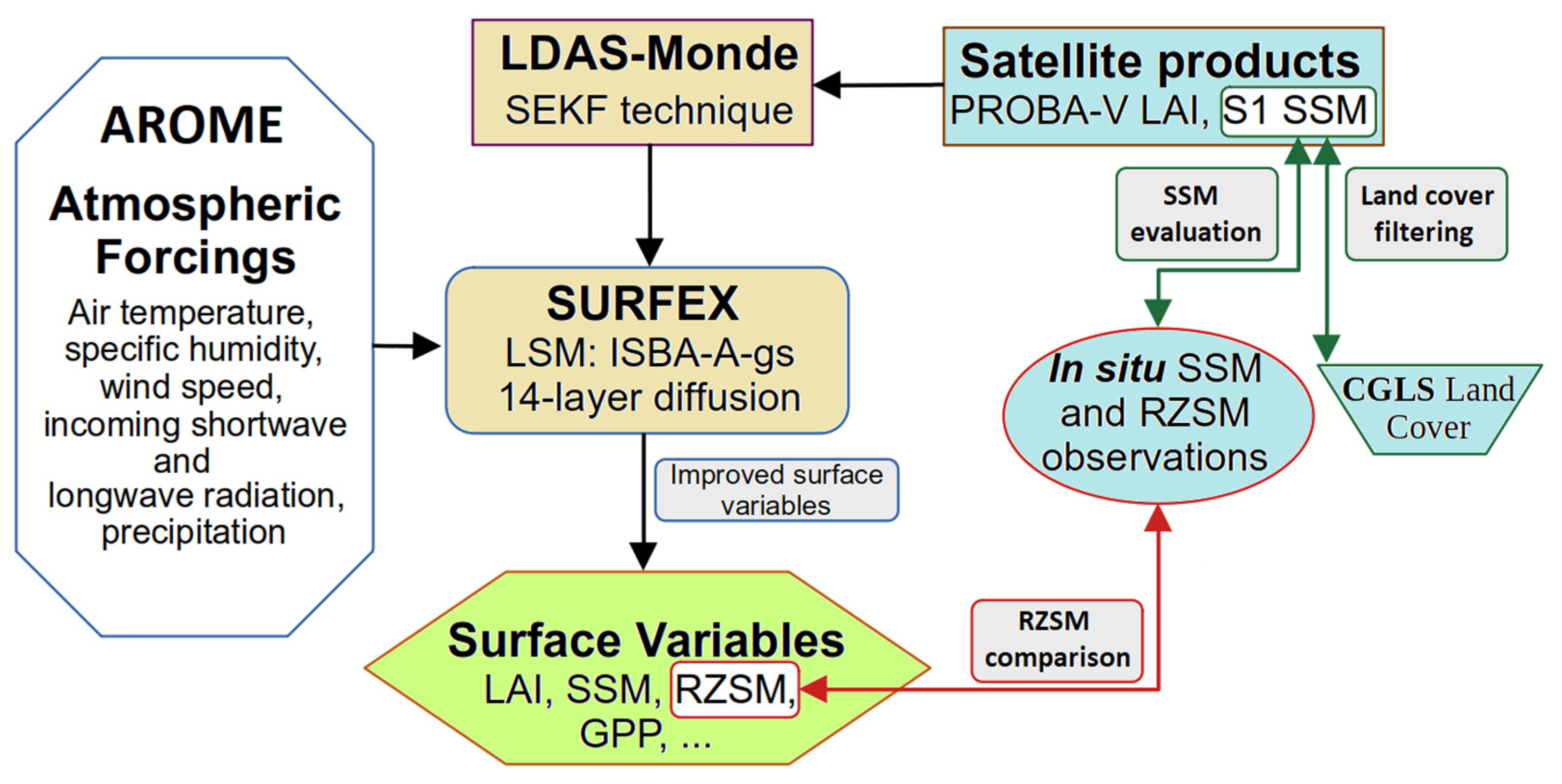
2.1. The ISBA LSM
2.2. LDAS-Monde
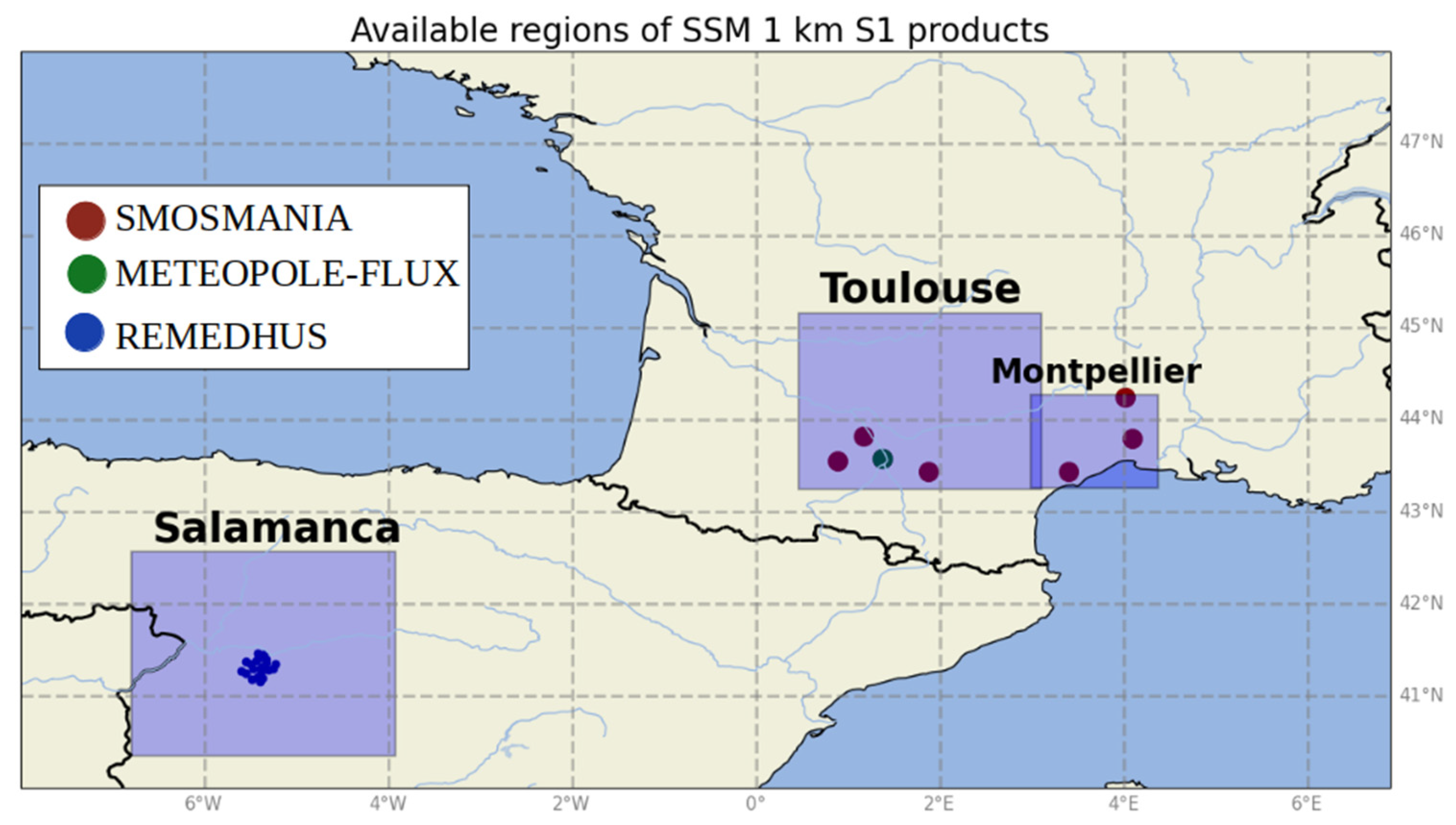
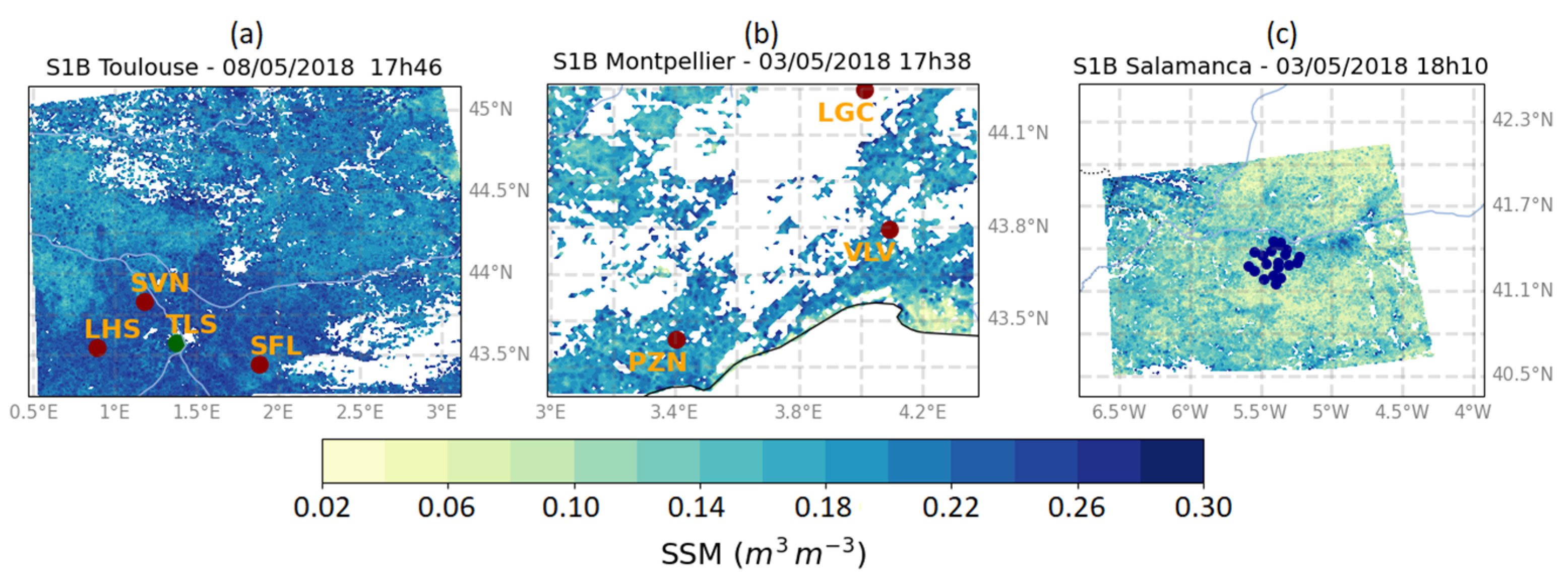
2.3. S1 SSM Data
2.4. LAI Data
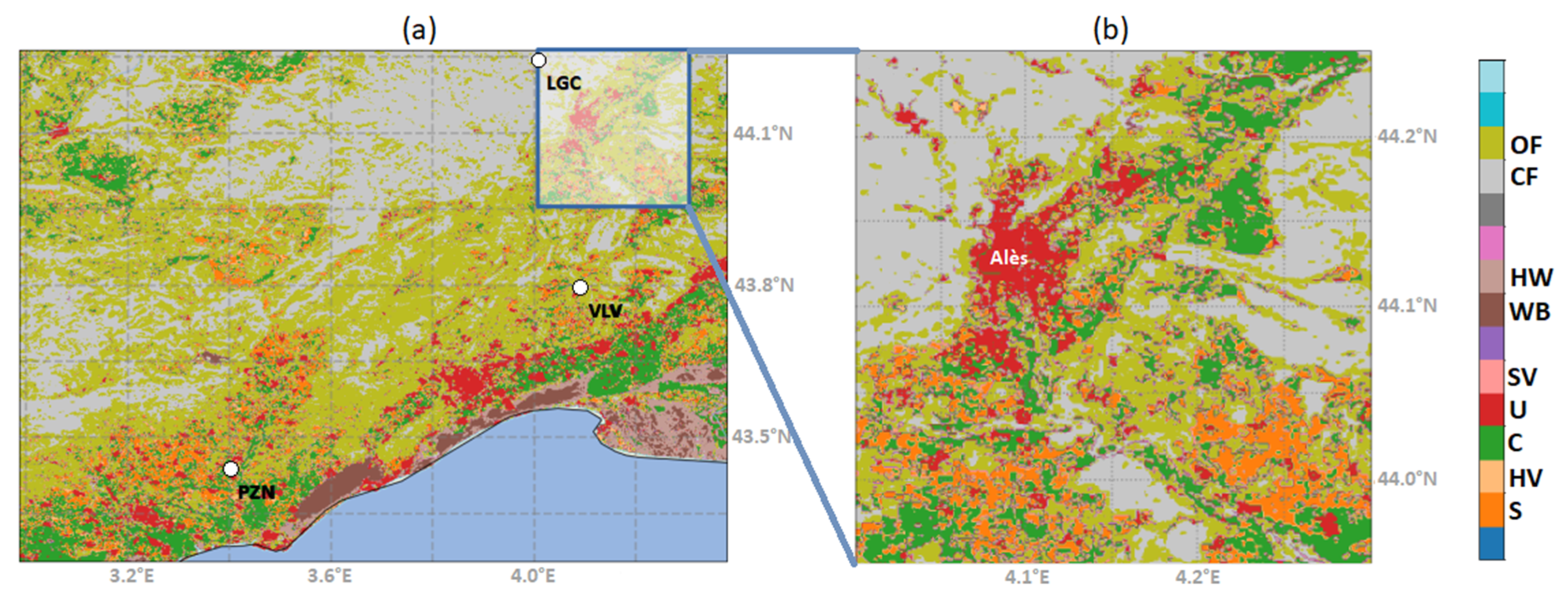
2.5. Land Cover
2.6. In Situ Observations
3. Method
3.1. Experimental Set Up
3.2. Evaluation
4. Results
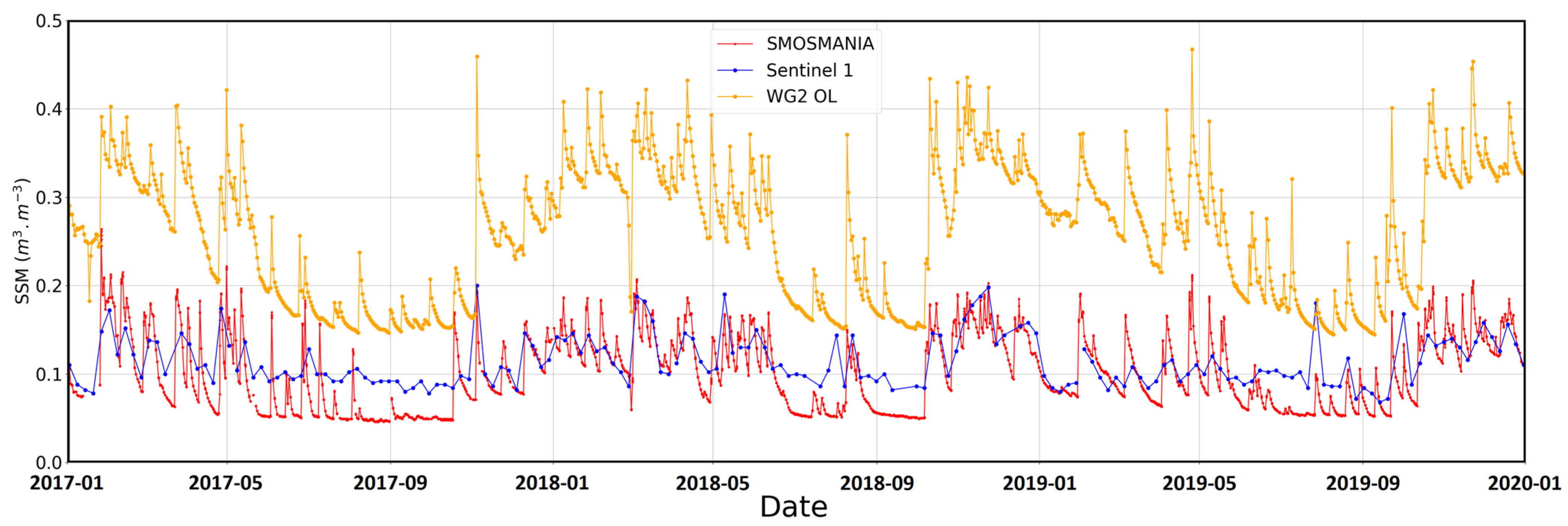
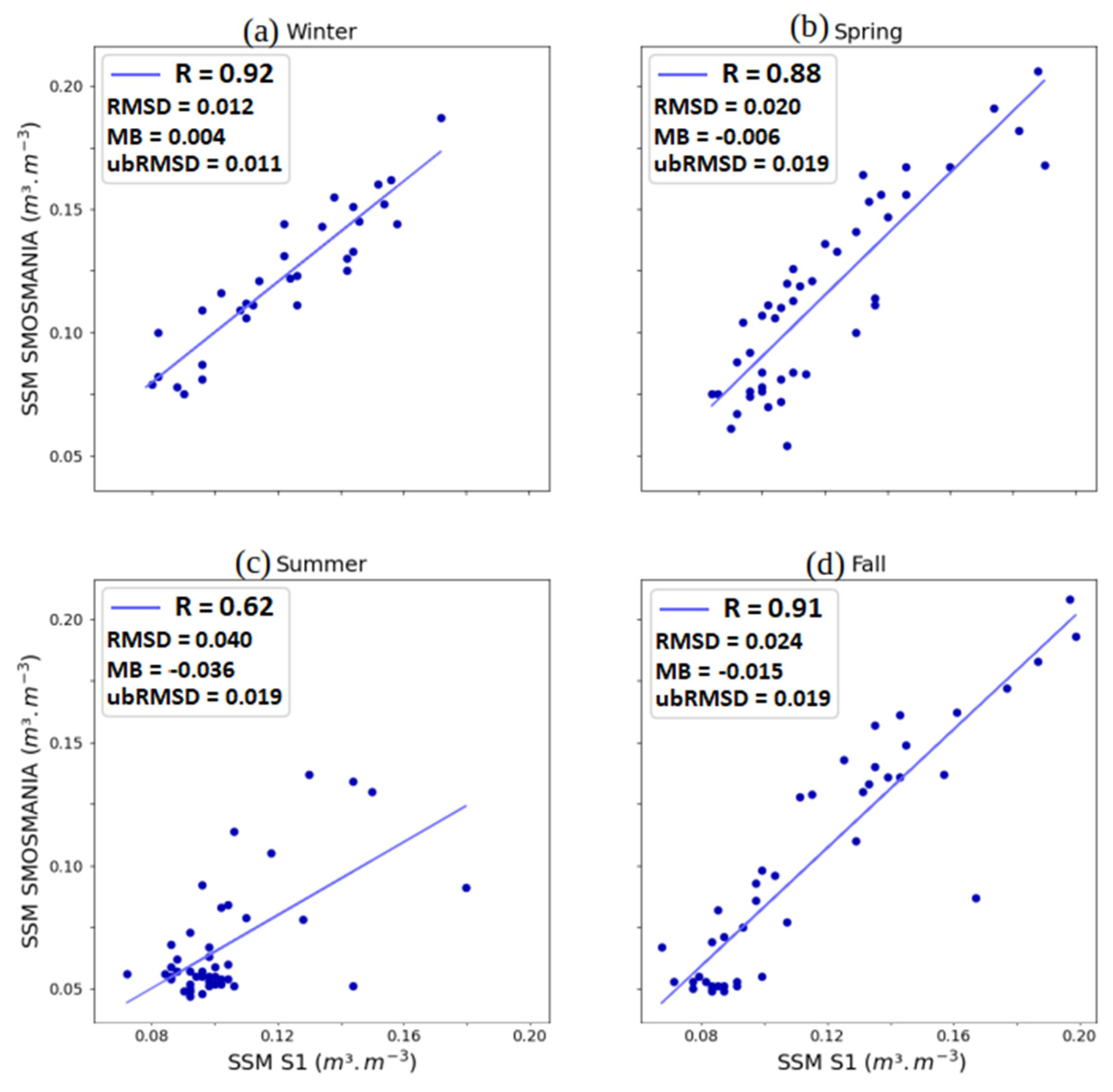
4.1. Validation of S1 SSM
4.2. Assimilation
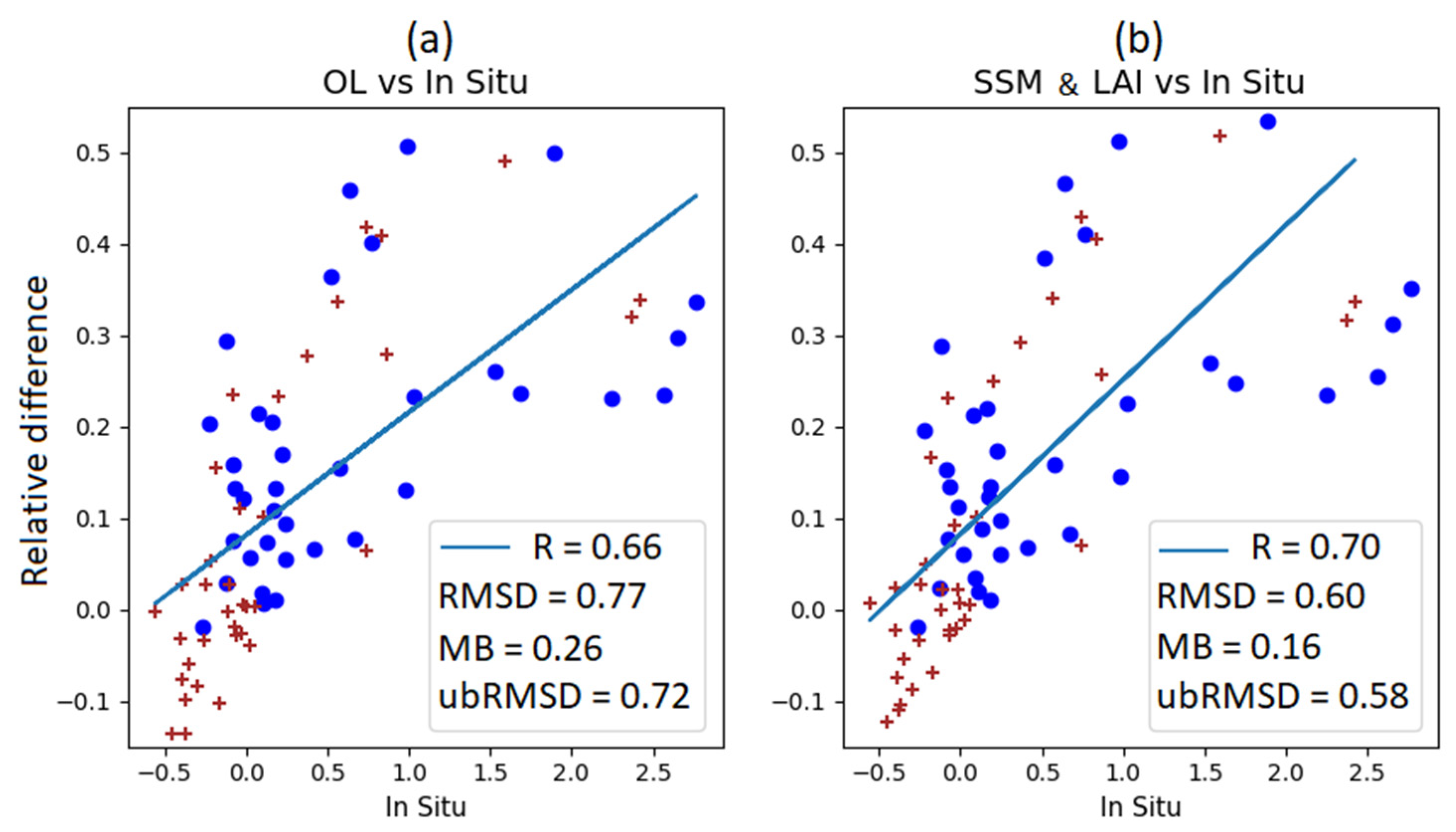
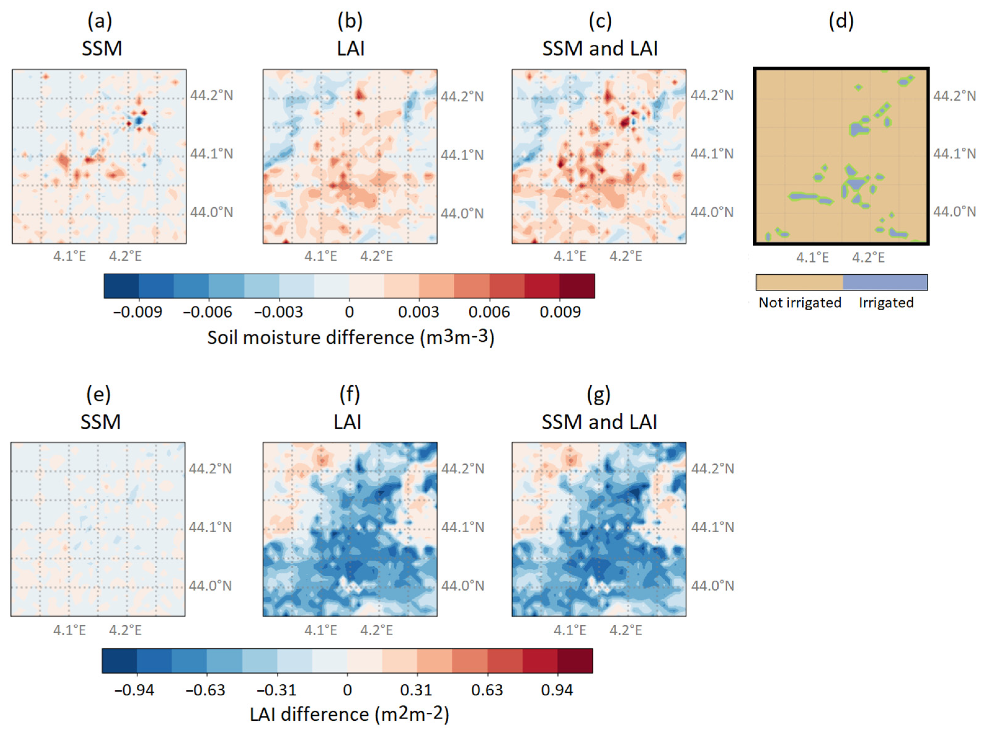
4.2.1. Local Comparison
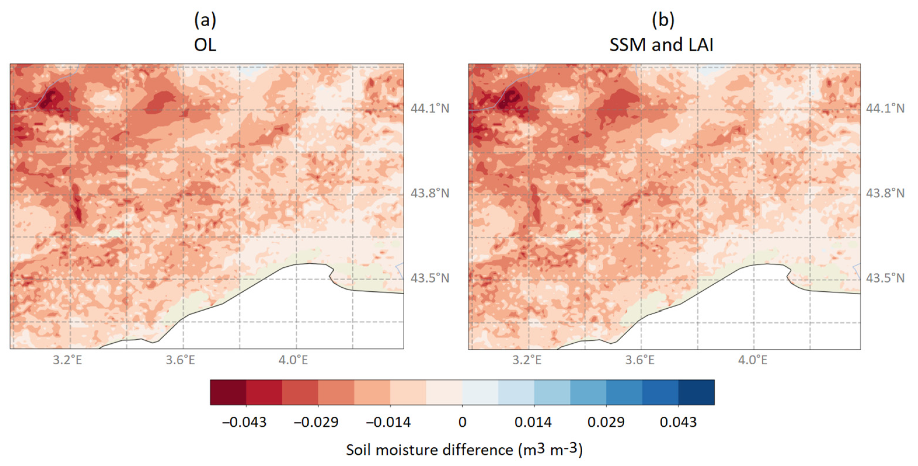
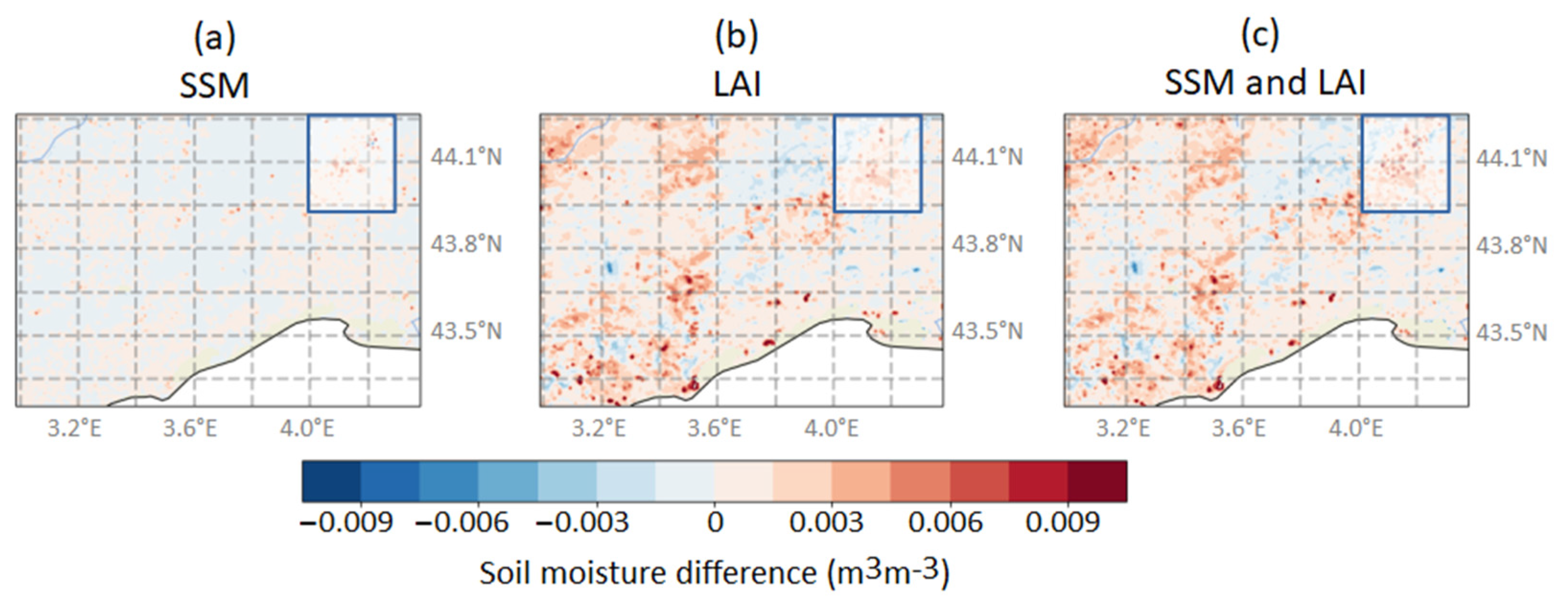
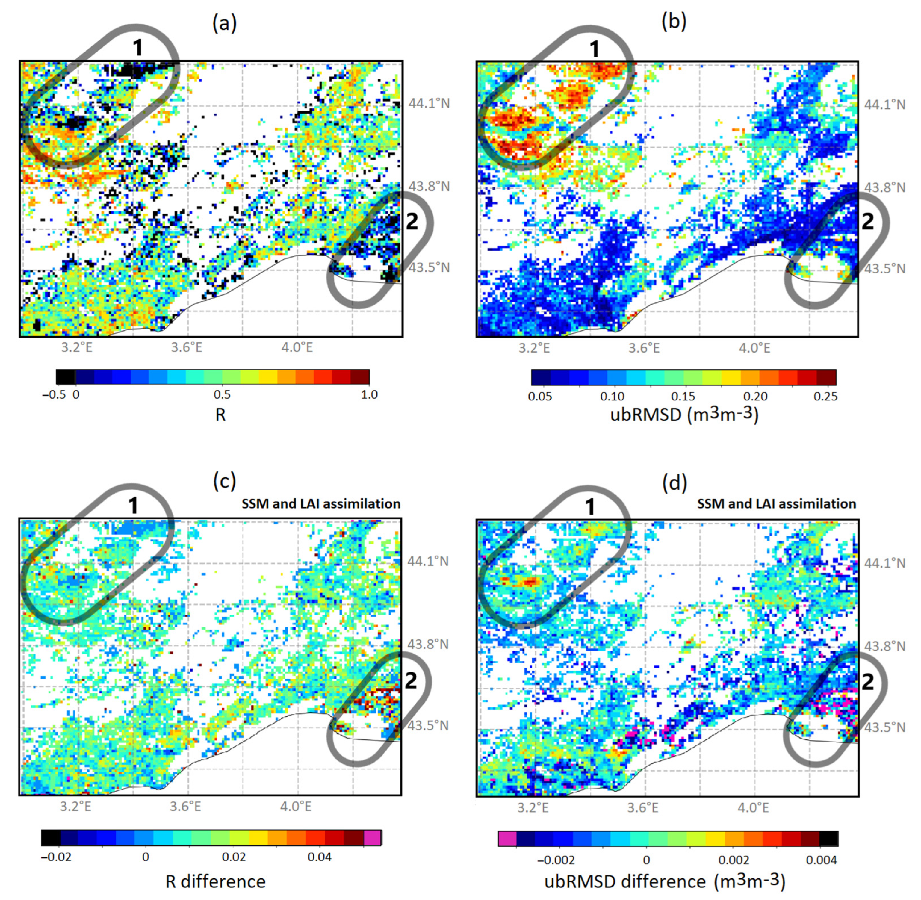
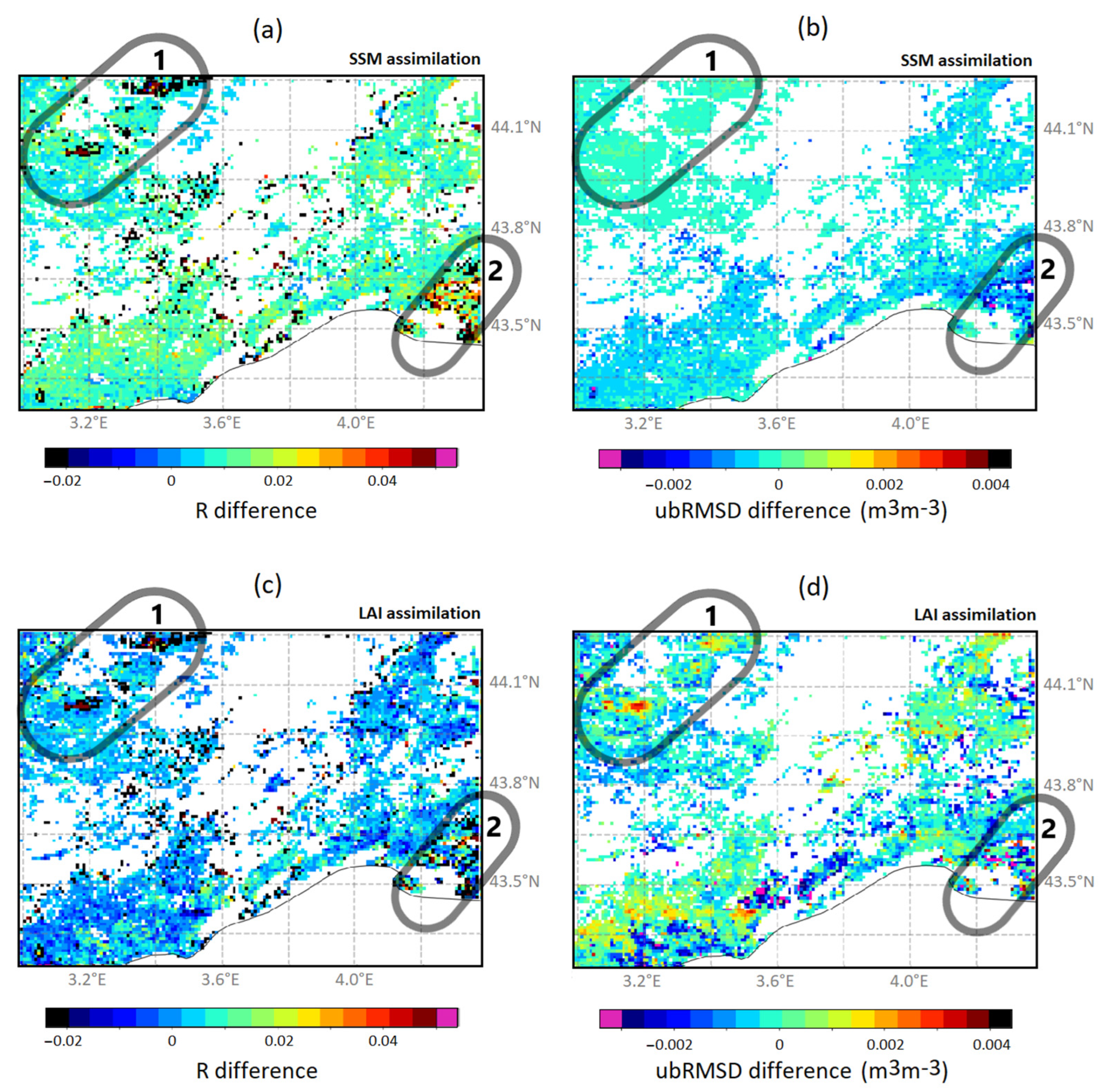
4.2.2. Regional Comparison
5. Discussion
5.1. Does S1 SSM Perform Better than Other SSM Products?
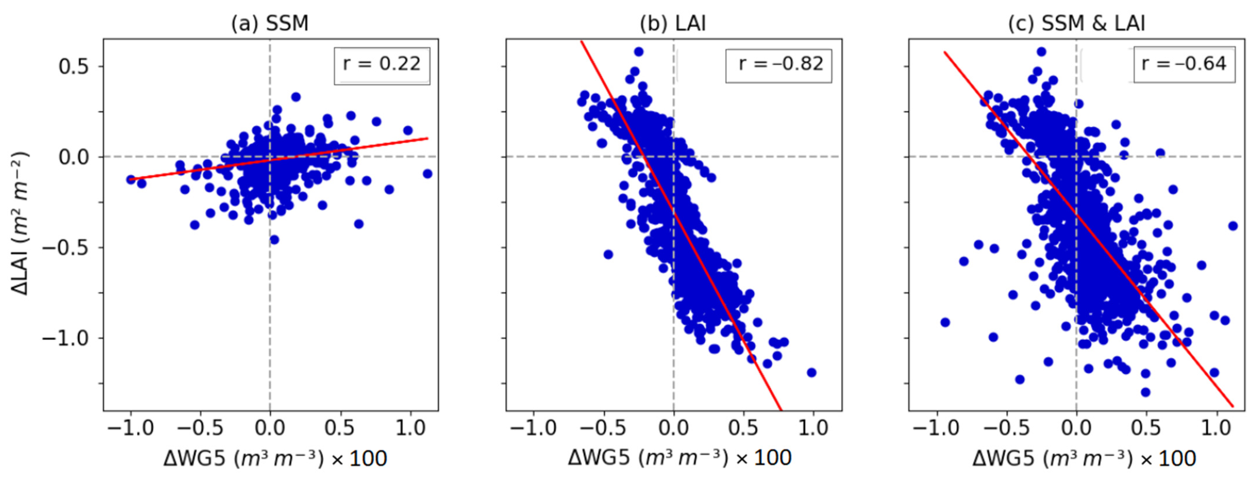
5.2. Why Is a Synergy of S1 SSM with LAI Observed in the Assimilation?
5.3. Can Geology and Land Use Affect the Assimilation?
6. Conclusions
Supplementary Materials
Author Contributions
Funding
Data Availability Statement
Acknowledgments
Conflicts of Interest
References
- Bartalis, Z.; Wagner, W.; Naeimi, V.; Hasenauer, S.; Scipal, K.; Bonekamp, H.; Figa, J.; Anderson, C. Initial Soil Moisture Retrievals from the METOP-A Advanced Scatterometer (ASCAT). Geophys. Res. Lett. 2007, 34, L20401. [Google Scholar] [CrossRef]
- Kerr, Y.H.; Waldteufel, P.; Wigneron, J.-P.; Delwart, S.; Cabot, F.; Boutin, J.; Escorihuela, M.-J.; Font, J.; Reul, N.; Gruhier, C.; et al. The SMOS mission: New tool for monitoring key elements of the global water cycle. Proc. IEEE 2010, 98, 666–687. [Google Scholar] [CrossRef]
- Massari, C.; Camici, S.; Ciabatta, L.; Brocca, L. Exploiting Satellite-Based Surface Soil Moisture for Flood Forecasting in the Mediterranean Area: State Update Versus Rainfall Correction. Remote Sens. 2018, 10, 292. [Google Scholar] [CrossRef]
- Sehgal, V.; Gaur, N.; Mohanty, B.P. Global Flash Drought Monitoring Using Surface Soil Moisture. Water Resour. Res. 2021, 57, e2021WR029901. [Google Scholar] [CrossRef]
- Seneviratne, S.I.; Corti, T.; Davin, E.L.; Hirschi, M.; Jaeger, E.B.; Lehner, I.; Orlowsky, B.; Teuling, A.J. Investigating Soil Moisture–Climate Interactions in a Changing Climate: A Review. Earth Sci. Rev. 2010, 99, 125–161. [Google Scholar] [CrossRef]
- Martínez-Fernández, J.; González-Zamora, A.; Sánchez, N.; Gumuzzio, A.; Herrero-Jiménez, C.M. Satellite Soil Moisture for Agricultural Drought Monitoring: Assessment of the SMOS Derived Soil Water Deficit Index. Remote Sens. Environ. 2016, 177, 277–286. [Google Scholar] [CrossRef]
- Wagner, W.; Blöschl, G.; Pampaloni, P.; Calvet, J.-C.; Bizzarri, B.; Wigneron, J.-P.; Kerr, Y. Operational Readiness of Microwave Remote Sensing of Soil Moisture for Hydrologic Applications. Hydrol. Res. 2007, 38, 1–20. [Google Scholar] [CrossRef]
- Peng, J.; Albergel, C.; Balenzano, A.; Brocca, L.; Cartus, O.; Cosh, M.H.; Crow, W.T.; Dabrowska-Zielinska, K.; Dadson, S.; Davidson, M.W.J.; et al. A Roadmap for High-Resolution Satellite Soil Moisture Applications—Confronting Product Characteristics with User Requirements. Remote Sens. Environ. 2021, 252, 112162. [Google Scholar] [CrossRef]
- Abbaszadeh, P.; Moradkhani, H.; Zhan, X. Downscaling SMAP radiometer soil moisture over the CONUS using an ensemble learning method. Water Resour. Res. 2019, 55, 324–344. [Google Scholar] [CrossRef]
- El Hajj, M.; Baghdadi, N.; Zribi, M.; Bazzi, H. Synergic Use of Sentinel-1 and Sentinel-2 Images for Operational Soil Moisture Mapping at High Spatial Resolution over Agricultural Areas. Remote Sens. 2017, 9, 1292. [Google Scholar] [CrossRef]
- El Hajj, M.; Baghdadi, N.; Wigneron, J.-P.; Zribi, M.; Albergel, C.; Calvet, J.-C.; Fayad, I. First Vegetation Optical Depth Mapping from Sentinel-1 C-band SAR Data over Crop Fields. Remote Sens. 2019, 11, 2769. [Google Scholar] [CrossRef]
- Foucras, M.; Zribi, M.; Albergel, C.; Baghdadi, N.; Calvet, J.-C.; Pellarin, T. Estimating 500-m Resolution Soil Moisture Using Sentinel-1 and Optical Data Synergy. Water 2020, 12, 866. [Google Scholar] [CrossRef]
- Madelon, R.; Rodríguez-Fernández, N.J.; Bazzi, H.; Baghdadi, N.; Albergel, C.; Dorigo, W.; Zribi, M. Soil moisture estimates at 1 km resolution making a synergistic use of Sentinel data. Hydrol. Earth Syst. Sci. 2023, 27, 1221–1242. [Google Scholar] [CrossRef]
- Dirmeyer, P.A.; Gao, X.; Zhao, M.; Guo, Z.; Oki, T.; Hanasaki, N. The Second Global Soil Wetness Project (GSWP-2): Multi-model analysis and implications for our perception of the land surface. Bull. Am. Meteorol. Soc. 2006, 87, 1381–1397. [Google Scholar] [CrossRef]
- Schellekens, J.; Dutra, E.; Martínez-de la Torre, A.; Balsamo, G.; van Dijk, A.; Sperna Weiland, F.; Minvielle, M.; Calvet, J.-C.; Decharme, B.; Eisner, S.; et al. A global water resources ensemble of hydrological models: The eartH2Observe Tier-1 dataset, Earth Syst. Sci. Data 2017, 9, 389–413. [Google Scholar] [CrossRef]
- Noilhan, J.; Mahfouf, J.-F. The ISBA Land Surface Parameterisation Scheme. Global Planet. Chang. 1996, 13, 145–159. [Google Scholar] [CrossRef]
- Calvet, J.-C.; Noilhan, J.; Roujean, J.-L.; Bessemoulin, P.; Cabelguenne, M.; Olioso, A.; Wigneron, J.-P. An Interactive Vegetation SVAT Model Tested against Data from Six Contrasting Sites. Agric. For. Meteorol. 1998, 92, 73–95. [Google Scholar] [CrossRef]
- Calvet, J.-C.; Rivalland, V.; Picon-Cochard, C.; Guehl, J.-M. Modelling forest transpiration and CO2 fluxes—Response to soil moisture stress. Agric. For. Meteorol. 2004, 124, 143–156. [Google Scholar] [CrossRef]
- Gibelin, A.-L.; Calvet, J.-C.; Roujean, J.-L.; Jarlan, L.; Los, S.O. Ability of the land surface model ISBA-A-gs to simulate leaf area index at the global scale: Comparison with satellites products. J. Geophys. Res. 2006, 111, D18102. [Google Scholar] [CrossRef]
- Albergel, C.; Rüdiger, C.; Pellarin, T.; Calvet, J.-C.; Fritz, N.; Froissard, F.; Suquia, D.; Petitpa, A.; Piguet, B.; Martin, E. From near-surface to root-zone soil moisture using an exponential filter: An assessment of the method based on in-situ observations and model simulations. Hydrol. Earth Syst. Sci. 2008, 12, 1323–1337. [Google Scholar] [CrossRef]
- Meng, X.; Wang, H.; Chen, J.; Yang, M.; Pan, Z. High-Resolution Simulation and Validation of Soil Moisture in the Arid Region of Northwest China. Sci. Rep. 2019, 9, 17227. [Google Scholar] [CrossRef] [PubMed]
- Swenson, S.C.; Lawrence, D.M.; Lee, H. Improved Simulation of the Terrestrial Hydrological Cycle in Permafrost Regions by the Community Land Model. J. Adv. Model. Earth Syst. 2012, 4, M08002. [Google Scholar] [CrossRef]
- Rasheed, M.W.; Tang, J.; Sarwar, A.; Shah, S.; Saddique, N.; Khan, M.U.; Imran Khan, M.; Nawaz, S.; Shamshiri, R.R.; Aziz, M.; et al. Soil Moisture Measuring Techniques and Factors Affecting the Moisture Dynamics: A Comprehensive Review. Sustainability 2022, 14, 11538. [Google Scholar] [CrossRef]
- Zhao, T.; Shi, J.; Lv, L.; Xu, H.; Chen, D.; Cui, Q.; Jackson, T.J.; Yan, G.; Jia, L.; Chen, L.; et al. Soil Moisture Experiment in the Luan River Supporting New Satellite Mission Opportunities. Remote Sens. Environ. 2020, 240, 111680. [Google Scholar] [CrossRef]
- Vather, T.; Everson, C.S.; Franz, T.E. The Applicability of the Cosmic Ray Neutron Sensor to Simultaneously Monitor Soil Water Content and Biomass in an Acacia mearnsii Forest. Hydrology 2020, 7, 48. [Google Scholar] [CrossRef]
- Pauwels, V.R.N.; Hoeben, R.; Verhoest, N.E.C.; De Troch, F.P.; Troch, P.A. Improvement of TOPLATS-Based Discharge Predictions through Assimilation of ERS-Based Remotely Sensed Soil Moisture Values. Hydrol. Process. 2002, 16, 995–1013. [Google Scholar] [CrossRef]
- Brocca, L.; Moramarco, T.; Melone, F.; Wagner, W.; Hasenauer, S.; Hahn, S. Assimilation of Surface- and Root-Zone ASCAT Soil Moisture Products into Rainfall–Runoff Modeling. IEEE Trans. Geosci. Remote Sens. 2012, 50, 2542–2555. [Google Scholar] [CrossRef]
- Fairbairn, D.; Barbu, A.L.; Napoly, A.; Albergel, C.; Mahfouf, J.-F.; Calvet, J.-C. The Effect of Satellite-Derived Surface Soil Moisture and Leaf Area Index Land Data Assimilation on Streamflow Simulations over France. Hydrol. Earth Syst. Sci. 2017, 21, 2015–2033. [Google Scholar] [CrossRef]
- Reichle, R.H.; Walker, J.P.; Koster, R.D.; Houser, P.R. Extended versus Ensemble Kalman Filtering for Land Data Assimilation. J. Hydrometeorol. 2002, 3, 728–740. [Google Scholar] [CrossRef]
- Draper, C.; Mahfouf, J.-F.; Calvet, J.-C.; Martin, E.; Wagner, W. Assimilation of ASCAT Near-Surface Soil Moisture into the SIM Hydrological Model over France. Hydrol. Earth Syst. Sci. 2011, 15, 3829–3841. [Google Scholar] [CrossRef]
- de Rosnay, P.; Drusch, M.; Vasiljevic, D.; Balsamo, G.; Albergel, C.; Isaksen, L. A simplified extended Kalman filter for the global operational soil moisture analysis at ECMWF. Q. J. R. Meteorol. Soc. 2013, 139, 1199–1213. [Google Scholar] [CrossRef]
- Barbu, A.L.; Calvet, J.-C.; Mahfouf, J.-F.; Albergel, C.; Lafont, S. Assimilation of Soil Wetness Index and Leaf Area Index into the ISBA-A-gs Land Surface Model: Grassland Case Study. Biogeosciences 2011, 8, 1971–1986. [Google Scholar] [CrossRef]
- Masson, V.; Le Moigne, P.; Martin, E.; Faroux, S.; Alias, A.; Alkama, R.; Belamari, S.; Barbu, A.; Boone, A.; Bouyssel, F.; et al. The SURFEXv7.2 Land and Ocean Surface Platform for Coupled or Offline Simulation of Earth Surface Variables and Fluxes. Geosci. Model Dev. 2013, 6, 929–960. [Google Scholar] [CrossRef]
- Albergel, C.; Munier, S.; Leroux, D.J.; Dewaele, H.; Fairbairn, D.; Barbu, A.L.; Gelati, E.; Dorigo, W.; Faroux, S.; Meurey, C.; et al. Sequential Assimilation of Satellite-Derived Vegetation and Soil Moisture Products Using SURFEX_v8.0: LDAS-Monde Assessment over the Euro-Mediterranean Area. Geosci. Model Dev. 2017, 10, 3889–3912. [Google Scholar] [CrossRef]
- Seity, Y.; Brousseau, P.; Malardel, S.; Hello, G.; Bénard, P.; Bouttier, F.; Lac, C.; Masson, V. The AROME-France Convective-Scale Operational Model. Mon. Weather Rev. 2011, 139, 976–991. [Google Scholar] [CrossRef]
- Brousseau, P.; Seity, Y.; Ricard, D.; Léger, J. Improvement of the forecast of convective activity from the AROME-France system. Q. J. R. Meteor. Soc. 2016, 142, 2231–2243. [Google Scholar] [CrossRef]
- Calvet, J.-C.; Gibelin, A.-L.; Roujean, J.-L.; Martin, E.; Le Moigne, P.; Douville, H.; Noilhan, J. Past and Future Scenarios of the Effect of Carbon Dioxide on Plant Growth and Transpiration for Three Vegetation Types of Southwestern France. Atmos. Chem. Phys. 2008, 8, 397–406. [Google Scholar] [CrossRef]
- Decharme, B.; Boone, A.; Delire, C.; Noilhan, J. Local Evaluation of the Interaction between Soil Biosphere Atmosphere Soil Multilayer Diffusion Scheme Using Four Pedotransfer Functions. J. Geophys. Res. D Atmos. 2011, 116, D20126. [Google Scholar] [CrossRef]
- Boone, A.; Masson, V.; Meyers, T.; Noilhan, J. The Influence of the Inclusion of Soil Freezing on Simulations by a Soil–Vegetation–Atmosphere Transfer Scheme. J. Appl. Meteorol. 2000, 39, 1544–1569. [Google Scholar] [CrossRef]
- Faroux, S.; Kaptué Tchuenté, A.T.; Roujean, J.-L.; Masson, V.; Martin, E.; Le Moigne, P. ECOCLIMAP-II/Europe: A Twofold Database of Ecosystems and Surface Parameters at 1 Km Resolution Based on Satellite Information for Use in Land Surface, Meteorological and Climate Models. Geosci. Model Dev. 2013, 6, 563–582. [Google Scholar] [CrossRef]
- Mucia, A.; Bonan, B.; Albergel, C.; Zheng, Y.; Calvet, J.-C. Assimilation of Passive Microwave Vegetation Optical Depth in LDAS-Monde: A Case Study over the Continental USA. Biogeosciences 2022, 19, 2557–2581. [Google Scholar] [CrossRef]
- Mucia, A.; Bonan, B.; Zheng, Y.; Albergel, C.; Calvet, J.-C. From Monitoring to Forecasting Land Surface Conditions Using a Land Data Assimilation System: Application over the Contiguous United States. Remote Sens. 2020, 12, 2020. [Google Scholar] [CrossRef]
- Leroux, D.J.; Calvet, J.-C.; Munier, S.; Albergel, C. Using Satellite-Derived Vegetation Products to Evaluate LDAS-Monde over the Euro-Mediterranean Area. Remote Sens. 2018, 10, 1199. [Google Scholar] [CrossRef]
- Albergel, C.; Munier, S.; Bocher, A.; Bonan, B.; Zheng, Y.; Draper, C.; Leroux, D.J.; Calvet, J.-C. LDAS-Monde Sequential Assimilation of Satellite Derived Observations Applied to the Contiguous US: An ERA-5 Driven Reanalysis of the Land Surface Variables. Remote Sens. 2018, 10, 1627. [Google Scholar] [CrossRef]
- Reichle, R.H.; Koster, R.D. Bias Reduction in Short Records of Satellite Soil Moisture. Geophys. Res. Lett. 2004, 31, L19501. [Google Scholar] [CrossRef]
- Drusch, M.; Wood, E.F.; Gao, H. Observation Operators for the Direct Assimilation of TRMM Microwave Imager Retrieved Soil Moisture. Geophys. Res. Lett. 2005, 32, L15403. [Google Scholar] [CrossRef]
- Scipal, K.; Holmes, T.; de Jeu, R.; Naeimi, V.; Wagner, W. A Possible Solution for the Problem of Estimating the Error Structure of Global Soil Moisture Data Sets. Geophys. Res. Lett. 2008, 35, L24403. [Google Scholar] [CrossRef]
- Barbu, A.L.; Calvet, J.-C.; Mahfouf, J.-F.; Lafont, S. Integrating ASCAT Surface Soil Moisture and GEOV1 Leaf Area Index into the SURFEX Modelling Platform: A Land Data Assimilation Application over France. Hydrol. Earth Syst. Sci. 2014, 18, 173–192. [Google Scholar] [CrossRef]
- Massari, C.; Brocca, L.; Tarpanelli, A.; Moramarco, T. Data Assimilation of Satellite Soil Moisture into Rainfall-Runoff Modelling: A Complex Recipe? Remote Sens. 2015, 7, 11403–11433. [Google Scholar] [CrossRef]
- Baret, F.; Weiss, M.; Lacaze, R.; Camacho, F.; Makhmara, H.; Pacholcyzk, P.; Smets, B. GEOV1: LAI and FAPAR Essential Climate Variables and FCOVER Global Time Series Capitalizing over Existing Products. Part1: Principles of Development and Production. Remote Sens. Environ. 2013, 137, 299–309. [Google Scholar] [CrossRef]
- Meier, J.; Zabel, F.; Mauser, W. A Global Approach to Estimate Irrigated Areas—A Comparison between Different Data and Statistics. Hydrol. Earth Syst. Sci. 2018, 22, 1119–1133. [Google Scholar] [CrossRef]
- Calvet, J.-C.; Fritz, N.; Berne, C.; Piguet, B.; Maurel, W.; Meurey, C. Deriving pedotransfer functions for soil quartz fraction in southern France from reverse modelling. Soil 2016, 2, 615–629. [Google Scholar] [CrossRef]
- Zhang, S.; Calvet, J.-C.; Darrozes, J.; Roussel, N.; Frappart, F.; Bouhours, G. Deriving surface soil moisture from reflected GNSS signal observations over a grassland site in southwestern France. Hydrol. Earth Syst. Sci. 2018, 22, 1931–1946. [Google Scholar] [CrossRef]
- Ceballos, A.; Scipal, K.; Wagner, W.; Martínez-Fernández, J. Validation of ERS Scatterometer-Derived Soil Moisture Data in the Central Part of the Duero Basin, Spain. Hydrol. Process. 2005, 19, 1549–1566. [Google Scholar] [CrossRef]
- Sanchez, N.; Martinez-Fernandez, J.; Scaini, A.; Perez-Gutierrez, C. Validation of the SMOS L2 Soil Moisture Data in the REMEDHUS Network (Spain). IEEE Trans. Geosci. Remote Sens. 2012, 50, 1602–1611. [Google Scholar] [CrossRef]
- Wagner, W.; Pathe, C.; Doubkova, M.; Sabel, D.; Bartsch, A.; Hasenauer, S.; Blöschl, G.; Scipal, K.; Martínez-Fernández, J.; Löw, A. Temporal Stability of Soil Moisture and Radar Backscatter Observed by the Advanced Synthetic Aperture Radar (ASAR). Sensors 2008, 8, 1174–1197. [Google Scholar] [CrossRef] [PubMed]
- Gonzalez-Zamora, A.; Sanchez, N.; Pablos, M.; Martinez-Fernandez, J. CCI soil moisture assessment with SMOS soil moisture and in situ data under different environmental conditions and spatial scales in Spain. Remote Sens. Environ. 2018, 225, 469–482. [Google Scholar] [CrossRef]
- Dorigo, W.; Himmelbauer, I.; Aberer, D.; Schremmer, L.; Petrakovic, I.; Zappa, L.; Preimesberger, W.; Xaver, A.; Annor, F.; Ardö, J.; et al. The International Soil Moisture Network: Serving Earth system science for over a decade. Hydrol. Earth Syst. Sci. 2021, 25, 5749–5804. [Google Scholar] [CrossRef]
- Owe, M.; Van de Griend, A.A. Comparison of soil moisture penetration depths for several bare soils at two microwave frequencies and implications for remote sensing. Water Resour. Res. 1998, 34, 2319–2327. [Google Scholar] [CrossRef]
- Albergel, C.; Zheng, Y.; Bonan, B.; Dutra, E.; Rodríguez-Fernández, N.; Munier, S.; Draper, C.; de Rosnay, P.; Muñoz-Sabater, J.; Balsamo, G.; et al. Data assimilation for continuous global assessment of severe conditions over terrestrial surfaces. Hydrol. Earth Syst. Sci. 2020, 24, 4291–4316. [Google Scholar] [CrossRef]
- Blauhut, V.; Stoelzle, M.; Ahopelto, L.; Brunner, M.I.; Teutschbein, C.; Wendt, D.E.; Akstinas, V.; Bakke, S.J.; Barker, L.J.; Bartošová, L.; et al. Lessons from the 2018–2019 European Droughts: A Collective Need for Unifying Drought Risk Management. Nat. Hazards Earth Syst. Sci. 2022, 22, 2201–2217. [Google Scholar] [CrossRef]
- EEA. Soil Moisture Dash Board, European Environment Agency. 2019. Available online: https://www.eea.europa.eu/data-and-maps/data/data-viewers/soil-moisture (accessed on 30 August 2023).
- Liu, Y.; Yang, Y.; Yue, X. Evaluation of satellite-based soil moisture products over four different continental in-situ measurements. Remote Sens. 2018, 10, 1161. [Google Scholar] [CrossRef]
- Feng, S.; Huang, X.; Zhao, S.; Qin, Z.; Fan, J.; Zhao, S. Evaluation of Several Satellite-Based Soil Moisture Products in the Continental US. Sensors 2022, 22, 9977. [Google Scholar] [CrossRef] [PubMed]
- Sishah, S.; Abrahem, T.; Azene, G.; Dessalew, A.; Hundera, H. Downscaling and Validating SMAP Soil Moisture Using a Machine Learning Algorithm over the Awash River Basin, Ethiopia. PLoS ONE 2023, 18, e0279895. [Google Scholar] [CrossRef] [PubMed]
- El Hajj, M.; Baghdadi, N.; Zribi, M.; Rodríguez-Fernández, N.; Wigneron, J.P.; Al-Yaari, A.; Al Bitar, A.; Albergel, C.; Calvet, J.-C. Evaluation of SMOS, SMAP, ASCAT and Sentinel-1 soil moisture products at sites in southwestern France. Remote Sens. 2018, 10, 569. [Google Scholar] [CrossRef]
- Portal, G.; Jagdhuber, T.; Vall-llossera, M.; Camps, A.; Pablos, M.; Entekhabi, D.; Piles, M. Assessment of multi-scale SMOS and SMAP soil moisture products across the Iberian peninsula. Remote Sens. 2020, 12, 570. [Google Scholar] [CrossRef]
- Tall, M.; Albergel, C.; Bonan, B.; Zheng, Y.; Guichard, F.; Dramé, M.S.; Gaye, A.T.; Sitondji, L.O.; Hountondji, F.C.C.; Nikiema, P.M.; et al. Towards a long-term reanalysis of land surface variables over western Africa: LDAS-Monde applied over Burkina Faso from 2001 to 2018. Remote Sens. 2019, 11, 735. [Google Scholar] [CrossRef]
- Capehart, W.; Carlson, T. Decoupling of surface and near-surface soil water content: A remote sensing perspective. Water Resour. Res. 1997, 33, 1383–1395. [Google Scholar] [CrossRef]
- Bonan, B.; Albergel, C.; Zheng, Y.; Barbu, A.L.; Fairbairn, D.; Munier, S.; Calvet, J.-C. An Ensemble Square Root Filter for the Joint Assimilation of Surface Soil Moisture and Leaf Area Index within the Land Data Assimilation System LDAS-Monde: Application over the Euro-Mediterranean Region. Hydrol. Earth Syst. Sci. 2020, 24, 325–347. [Google Scholar] [CrossRef]
- Bazzi, H.; Baghdadi, N.; El Hajj, M.; Zribi, M.; Belhouchette, H. A Comparison of Two Soil Moisture Products S2MP and Copernicus-SSM over Southern France. IEEE J. Sel. Top. Appl. Earth Obs. Remote Sens. 2019, 12, 3366–3375. [Google Scholar] [CrossRef]
- Modanesi, S.; Massari, C.; Bechtold, M.; Lievens, H.; Tarpanelli, A.; Brocca, L.; Zappa, L.; De Lannoy, G.J.M. Challenges and benefits of quantifying irrigation through the assimilation of Sentinel-1 backscatter observations into Noah-MP. Hydrol. Earth Syst. Sci. 2022, 26, 4685–4706. [Google Scholar] [CrossRef]
- Draper, C.S.; Reichle, R.H.; De Lannoy, G.J.M.; Liu, Q. Assimilation of Passive and Active Microwave Soil Moisture Retrievals. Geophys. Res. Lett. 2012, 39, L04401. [Google Scholar] [CrossRef]
- Wagner, W.; Lindorfer, R.; Melzer, T.; Hahn, S.; Bauer-Marschallinger, B.; Morrison, K.; Calvet, J.C.; Hobbs, S.; Quast, R.; Greimeister-Pfeil, I.; et al. Widespread occurrence of anomalous C-band backscatter signals in arid environments caused by subsurface scattering. Remote Sens. Environ. 2022, 276, 113025. [Google Scholar] [CrossRef]
- Shamambo, D.; Bonan, B.; Calvet, J.-C.; Albergel, C.; Hahn, S. Interpretation of ASCAT radar scatterometer observations over land: A case study over southwestern France. Remote Sens. 2019, 11, 2842. [Google Scholar] [CrossRef]


| Experiment | Assimilated Observations | Model Equivalent | Control Variables |
|---|---|---|---|
| OL | n/a | n/a | n/a |
| SSM | S1 SSM (rescaled) | WG2 (1–4 cm) | LAI, WG2 to WG8 (0.01–1 m) |
| LAI | PROBA-V LAI | LAI | LAI, WG2 to WG8 (0.01–1 m) |
| SSM and LAI | S1 SSM (rescaled) and PROBA-V LAI | WG2 (1–4 cm), LAI | LAI, WG2 to WG8 (0.01–1 m) |
| Comparison | R | ubRMSD (m³ m−3) | RMSD (m³ m−3) | MB (m³ m−3) | Number |
|---|---|---|---|---|---|
| OL vs. in situ | 0.87 | 0.043 | 0.165 | 0.159 | 165 |
| S1 SSM vs. in situ | 0.85 | 0.024 | 0.028 | −0.013 | 163 |
| S1 SSM vs. OL | 0.71 | 0.058 | 0.156 | −0.145 | 164 |
| SSM Product, Spatial Resolution, Reference | Region, Soil Moisture Network, Period | Average R | Average ubRMSD (m³ m−3) | Number of Stations |
|---|---|---|---|---|
| S1, 1 km, this study | Toulouse, SMOSMANIA, 2017–2019 | 0.57 | 0.072 | 4 |
| S1, 1 km, this study | Montpellier, SMOSMANIA, 2017–2019 | 0.64 | 0.05 | 3 |
| S1, 1 km, this study | Salamanca, REMEDHUS, 2017–2019 | 0.48 | 0.053 | 19 |
| S1, 1 km, [66] | Southern France (SMOSMANIA and Montpellier), 2016–2017 | 0.59 | 0.056 | 8 |
| SMAP-S1, 1 km, [66] | Southern France (SMOSMANIA and Montpellier), 2016–2017 | 0.48 | 0.043 | 8 |
| SMAP-S1, 1 km, [67] | Salamanca, REMEDHUS (rainfed crops only), 2015–2017 | 0.86 | 0.04 | 7 |
| ASCAT, 25 km, [66] | Southern France (SMOSMANIA and Montpellier), 2016–2017 | 0.49 | 0.062 | 8 |
| SMOS-IC, 25 km, [66] | Southern France (SMOSMANIA and Montpellier), 2016–2017 | 0.57 | 0.053 | 8 |
| SMOS, 25 km, [67] | Salamanca, REMEDHUS, 2015–2017 | 0.65 | 0.062 | 6 |
| SMAP, 36 km, [66] | Southern France (SMOSMANIA and Montpellier), 2016–2017 | 0.69 | 0.047 | 8 |
| SMAP, 36 km, [67] | Salamanca, REMEDHUS, 2015–2017 | 0.7 | 0.058 | 6 |
Disclaimer/Publisher’s Note: The statements, opinions and data contained in all publications are solely those of the individual author(s) and contributor(s) and not of MDPI and/or the editor(s). MDPI and/or the editor(s) disclaim responsibility for any injury to people or property resulting from any ideas, methods, instructions or products referred to in the content. |
© 2023 by the authors. Licensee MDPI, Basel, Switzerland. This article is an open access article distributed under the terms and conditions of the Creative Commons Attribution (CC BY) license (https://creativecommons.org/licenses/by/4.0/).
Share and Cite
Rojas-Munoz, O.; Calvet, J.-C.; Bonan, B.; Baghdadi, N.; Meurey, C.; Napoly, A.; Wigneron, J.-P.; Zribi, M. Soil Moisture Monitoring at Kilometer Scale: Assimilation of Sentinel-1 Products in ISBA. Remote Sens. 2023, 15, 4329. https://doi.org/10.3390/rs15174329
Rojas-Munoz O, Calvet J-C, Bonan B, Baghdadi N, Meurey C, Napoly A, Wigneron J-P, Zribi M. Soil Moisture Monitoring at Kilometer Scale: Assimilation of Sentinel-1 Products in ISBA. Remote Sensing. 2023; 15(17):4329. https://doi.org/10.3390/rs15174329
Chicago/Turabian StyleRojas-Munoz, Oscar, Jean-Christophe Calvet, Bertrand Bonan, Nicolas Baghdadi, Catherine Meurey, Adrien Napoly, Jean-Pierre Wigneron, and Mehrez Zribi. 2023. "Soil Moisture Monitoring at Kilometer Scale: Assimilation of Sentinel-1 Products in ISBA" Remote Sensing 15, no. 17: 4329. https://doi.org/10.3390/rs15174329