Remote Sensing-Based Approach for the Assessing of Ecological Environmental Quality Variations Using Google Earth Engine: A Case Study in the Qilian Mountains, Northwest China

Abstract

Due to climate change and human activities, the eco-environment quality (EEQ) of eco-fragile regions has undergone massive change, especially in the Tibet Plateau. The Qilian Mountains (QLM) region is an essential ecological function zone in the northeastern Tibet Plateau, which plays a vital role in northwestern China’s eco-environmental balance. However, EEQ changes in the QLM during the 21st century remain poorly understood. In this study, the spatiotemporal variations of the EEQ in the QLM were analyzed from 2000 to 2020 using a remote sensing ecological index (RSEI). The EEQ driving factors are identified by the geographic detector, and the spatial influence of critical factors is represented by a geographically weighted regression model. The results show low EEQ in the QLM. From 2000 to 2020, the EEQ initially slightly improved, then deteriorated, and finally gradually recovered. Spatially, the EEQ shows an increasing trend from northwest to southeast. Moran’s I of EEQ remains at around 0.95, representing high spatial aggregation. “High–High” and “Low–Low” clustering features dominate in the local spatial autocorrelation, indicating the EEQ of the QLM is polarized. Precipitation is the dominant positive factor in the EEQ, with a q statistics exceeding 0.644. Furthermore, the key factors (precipitation, distance to towns, distance to roads) affecting EEQ in different periods vary significantly in space. From results we can draw the conclusion that the natural factors mainly control the spatial patterns of EEQ, while the human factors mainly impact the temporal trend of EEQ, the EEQ in the QLM has been significantly improved since 2015. Our findings can provide theoretical support for future eco-environmental protection and restoration in the QLM.

1. Introduction

As a result of economic growth, increasing human activities, and climate change, the global eco-environment has changed significantly in recent decades, especially in regions with fragile environments [1]. In this context, once the ecological environmental quality (EEQ) decreases to a certain level, many eco-environmental problems arise, including biodiversity decline, grassland degradation, soil erosion, and ecosystem service damage [2,3]. Thus, it is necessary to systematically evaluate EEQ and analyze its driving mechanisms to identify existing problems and further protect ecological integrity.

However, timely and quantitatively assessments of EEQ are challenging due to the links between EEQ and multiple driving factors, in addition to its structural complexity and spatiotemporal variability in ecosystem functions [4]. Nonetheless, it is urgent to systematically evaluate EEQ to formulate socioeconomic sustainable development plans and eco-environmental protection approaches [5]. In recent years, remote sensing has become an effective method to investigate spatiotemporal changes in EEQ at different scales due to the high efficiency, accuracy, availability, and low cost of remote sensing data [6]. Many studies have used a single ecological indicator from remote sensing to investigate eco-environment status; for example, the normalized difference vegetation index (NDVI) is often used as a single ecological indicator to assess vegetation coverage [7,8]. However, it is difficult to fully reflect the EEQ of eco-fragile regions using a single indicator given the complexity of its ecosystem.

To consider the ecosystem comprehensively, integrated remote sensing-based ecological indicators have also been applied [9,10]. In 2006, the Ministry of Environmental Protection of China issued the eco-environment evaluation technical specifications as an industry standard. These specifications propose a remote sensing-based ecological index (EI), which is widely used for eco-environment evaluation at the county level in China [11]. However, EI evaluation is greatly affected by expert experience and knowledge; in addition, there are still numerous problems involved in developing remote sensing-based indicators and weights [12,13]. Some researchers have aimed to develop an integrated ecological index to objectively reflect EEQ. Xu [14] developed a remote sensing ecological index (RSEI) that relies entirely on remote sensing technology to integrate multiple factors and that can comprehensively reflect the ecological status at different regional scales. The RSEI incorporates four important remote sensing-based ecological indicators (greenness, wetness, dryness, and heat) by using principal component analysis (PCA) [8,15]. RSEI overcomes the limitations of using a single indicator, makes the integration of sub-indicators objective and reasonable, and avoids the need for subjective manual settings, which are widely used in other studies [16,17,18,19]. Therefore, the RSEI can be reliably applied to rapidly evaluate the EEQ.

EEQ changes are linked to several factors, including topography, climate, human activities, and policy. It is vital to understand the change characteristics and factors influencing EEQ to identify conflicts between economic development and ecosystem health [20]. To date, researchers have applied various methods to explore the impact of potential EEQ driving factors, such as multiple linear regression [17], gray relational analysis [21], and forward stepwise linear regression [19]. However, these methods generally do not quantify the relative importance of different EEQ driving factors and do not consider spatial differences in these factors. Furthermore, these methods disregard the spatial non-stationarity and autocorrelation of driving factors in a region; therefore, these are key limitations to the results obtained from above methods [22].

To gain deeper insights into EEQ changes, it is necessary to consider the contributions and interactions of various driving factors. The geographical detector (GeoDetector) method, as proposed by Wang et al. [23] can be used to quantify the contributions of independent variables to the dependent variables. This approach has been widely used to determine the factors influencing vegetation change [7], ecosystem services [24], and soil organic carbon [25]. Additionally, the distributions of EEQ and its driving factors are spatial heterogeneous. The geographically weighted regression (GWR) model can be used to explain the spatial heterogeneity between the independent variables and the dependent variables [13,26]. Accordingly, this study combines the GeoDetector and GWR models to comprehensively explore the impact intensity and spatial variability of natural and anthropogenic factors on EEQ.

The Qilian Mountains (QLM) region is located in Northwest China. This area contains the headwaters of three important inland rivers in the Hexi Corridor region: the Heihe, Shiyanghe, and Shulehe rivers [27]. However, increasing levels of human activity, including mining, hydropower construction, and tourism development, have caused severe damage to the area’s eco-environment [2]. These activities not only impact ecosystem stability in the QLM but also threaten sustainable development of the eco-environment. To address these eco-environmental problems, the Chinese government has successively established National Nature Reserves and National Parks in the QLM and implemented ecological projects such as returning farmland to forests and grasslands and the “Three North” Shelterbelt Project. These projects and policies may have profound effects on the eco-environment of the QLM, which may result in EEQ changes. Thus, it is urgent to evaluate the EEQ of the QLM for eco-environmental protection.

The main aim of this study is to quantitatively represent the spatiotemporal distribution of EEQ and explore its main driving factors using a combination of GeoDetector and GWR models. Specifically, the study’s objectives are to: (1) evaluate spatiotemporal distributions of EEQ in the QLM from 2000 to 2020; (2) explore the dynamic change characteristics of EEQ; (3) quantify the relative importance of various impact factors and their interactions on the EEQ; and (4) analyze the spatial differences of key factors driving EEQ changes. The results of this study are expected to provide an important scientific basis for protecting and managing eco-environments in the QLM.

2. Materials and Methods

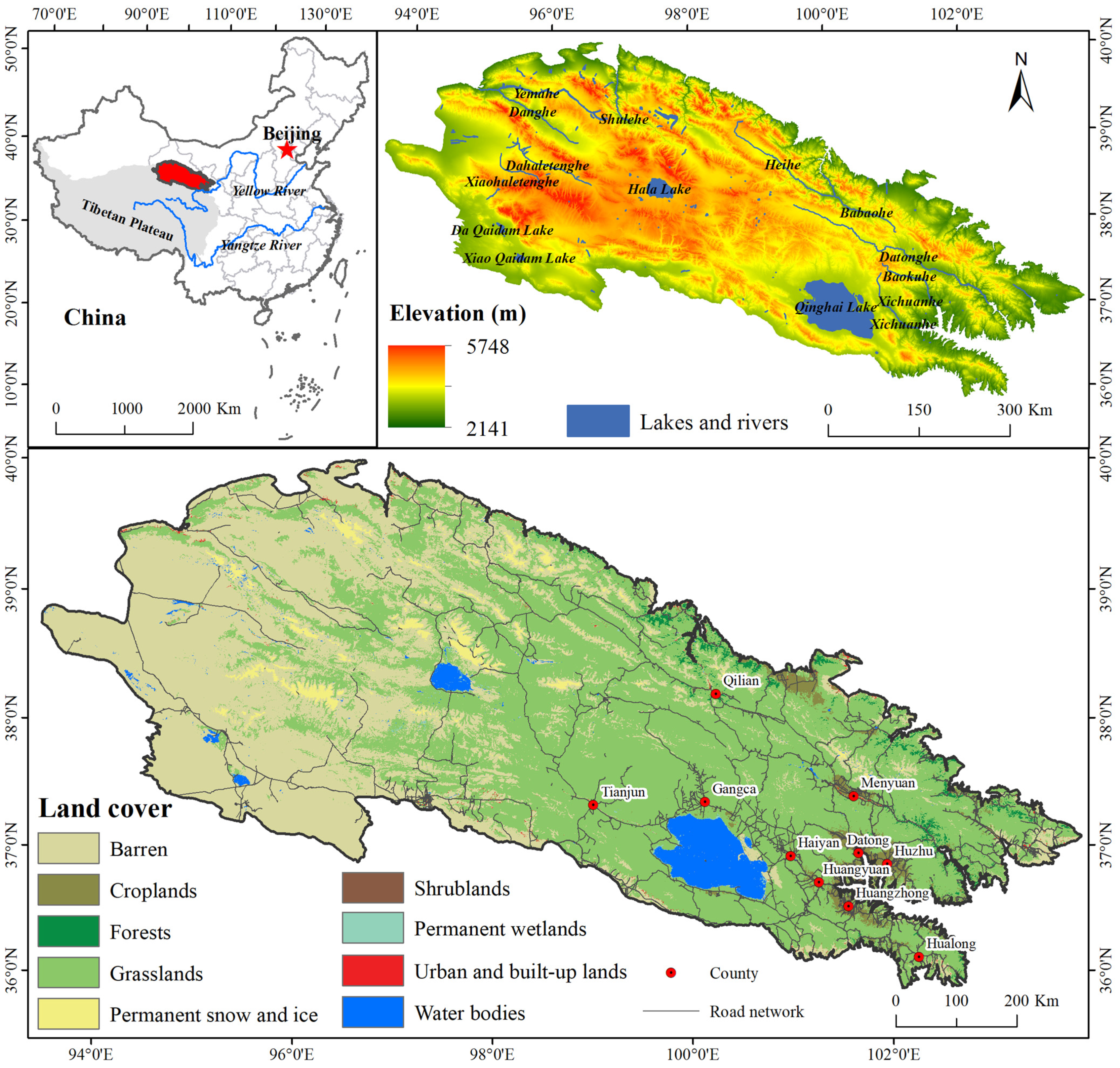
2.1. Study Area

The QLM region (35.8–40°N and 93.3–103.9°E), a typical alpine area, is located on the northeastern edge of the Qinghai–Tibet Plateau, which is known as the “roof of the world”. The QLM area extends approximately 1000 km from the southeast to the northwest, covering around 184,000 km² (Figure 1). Administratively, the QLM region belongs to Gansu and Qinghai provinces in northwest China. The overall terrain of the QLM is higher in the west and lower in the east. The elevation ranges from 2141 m to 5748 m, with an average value of 3500 m above sea level. This area has a typical plateau continental climate, with a mean annual temperature of −0.8 °C, and annual precipitation ranging from 150 mm to 800 mm, increasing from west to east [28]. Grassland covers the largest fraction of the QLM, accounting for 53.45% of the total area. Barren land occupies the second-largest area (40.15%) and mostly occurs in the western QLM [29]. The QLM region has complex topographic and climatic conditions, and the area’s natural ecosystem is fragile and sensitive to climate change and human activities [30]. In addition, many mining and waterpower resources are present in the region. Such resource exploitation causes regional vegetation damage, water quality degradation, and environmental pollution [31]. In this context, eco-environmental issues in the QLM have received widespread attention. To prevent degradation of the area’s eco-environment, the Qilian Mountain National Park was established in 2018. Therefore, we hope that this case study of spatiotemporal EEQ changes in the QLM will provide a reference for investigating and preserving other similarly fragile areas.

2.2. Data Source and Preprocessing

2.2.1. RSEI Datasets

Moderate Resolution Imaging Spectroradiometer (MODIS) images have been widely used to monitor ecological status at large regional scales [19]. According to the RSEI construction framework proposed by Xu [14], greenness, wetness, dryness, and heat are the four ecological components of RSEI, which can be described by the NDVI, wetness index (WET), normalized difference build-up and soil index (NDBSI), and land surface temperature (LST), respectively. To obtain the four indexes, three types of MODIS V6 datasets were used in this study: MOD13A1 to obtain NDVI (500 m and 16-day), MOD09A1 (500 m and 8-day) to calculate WET and NDBSI, and MOD11A2 to obtain the LST (1000 m and 8-day). To avoid the uncertainty caused by seasonal changes, we selected MODIS images from the optimal growing season (June–August) each year from 2000 to 2020. The MOD13A1 NDVI dataset was combined using the maximum value composite method. For the MOD09A1 dataset, we first used the quality layer to remove cloud and fog to synthesize high-quality images, which were then used to calculate the WET and NDBSI. The MOD11A2 LST product was obtained by calculating the average value of LST for each year. All preprocessing of MODIS images and the calculation of four indexes were performed on the Google Earth Engine (GEE) platform (https://earthengine.google.org, accessed on 30 December 2022).

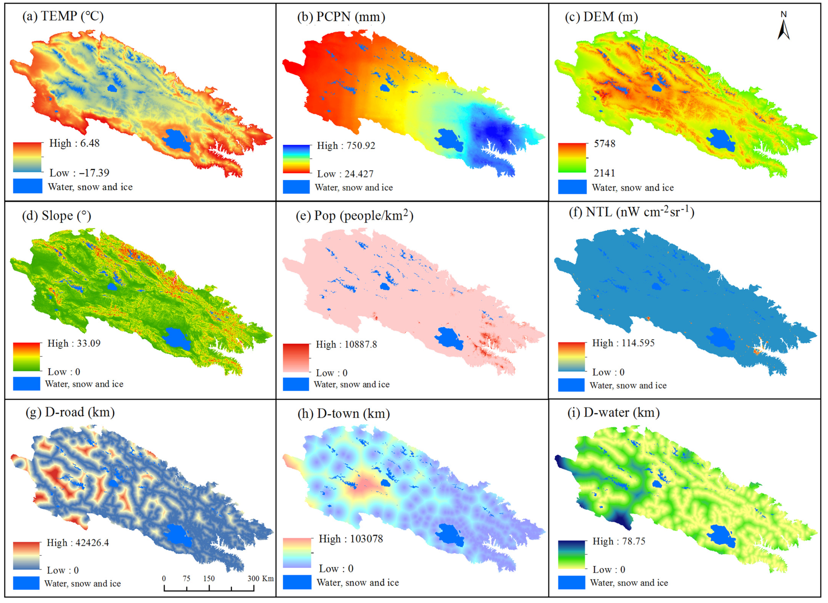
2.2.2. Driving Factor Datasets

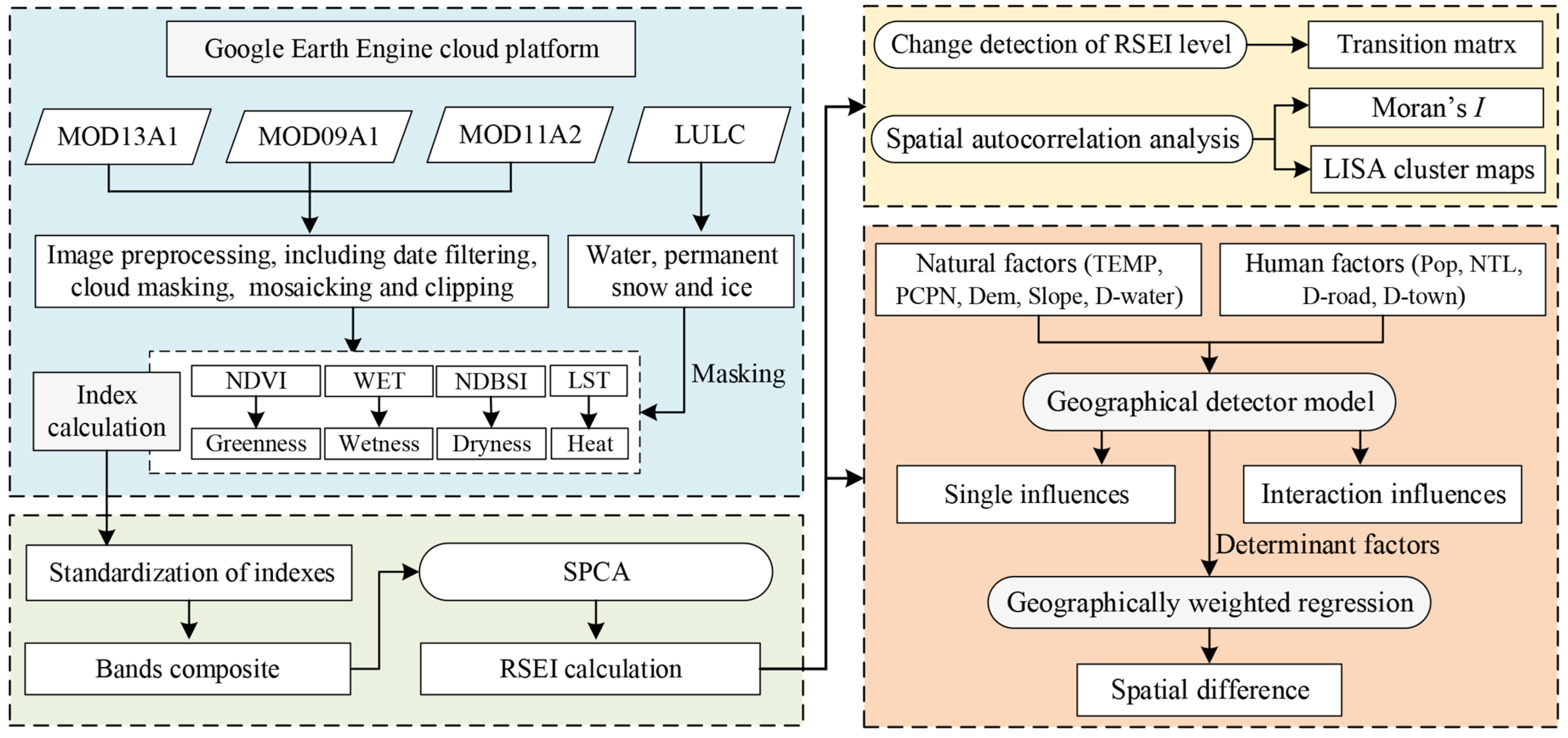
EEQ changes are comprehensively affected by natural conditions and human activity. To identify the factors driving EEQ changes, we selected nine factors based on the features of the QLM and previous studies [32,33] (

Table 1. Driving factors preprocessed in this study.

Factor Type	Variables	Unit	Abbreviation	Data Description	Data Source
Natural factors	Temperature	°C	TEMP	Raster, 1 km	http://www.geodata.cn/data/, (accessed on 30 December 2022)
	Precipitation	mm	PCPN	Raster, 1 km	Wang et al. [34]
	Digital elevation model	m	Dem	Raster, 90 m	http://www.gscloud.cn/, (accessed on 30 December 2022)
	Slope	°	Slope	Raster, 90 m	Extracted from DEM
	Distance to water sources	km	D-water	Raster, 1 km	https://www.openstreetmap.org, (accessed on 30 December 2022)
Human factors	Population density	people/km2	Pop	Raster, 1 km	https://www.worldpop.org, (accessed on 30 December 2022)
	Nighttime light intensity	nW cm−2 sr−1	NTL	Raster, 500m	https://doi.org/10.7910/DVN/YGIVCD, (accessed on 30 December 2022)
	Distance to roads	km	D-road	Raster, 1 km	https://www.openstreetmap.org, (accessed on 30 December 2022)
	Distance to towns	km	D-town	Raster, 1 km

). The natural factors include temperature, precipitation, altitude, slope, and distance to water sources. The temperature data were derived from a dataset released by the National Earth System Science Data Center. The precipitation data are the downscaled Global Satellite Mapping of Precipitation (GSMap) dataset for the QLM from our previous work [34]. The digital elevation model (DEM) data were derived from the Geospatial Data Cloud Platform, from which the slope values were extracted. The human factors explored in this study include population density, nighttime light intensity, distance to roads, and distance to towns. The population density data were obtained from the WorldPop Project. The nighttime light data were obtained from a dataset corrected and published by Chen et al. [35]. The water source, road, and town data were downloaded from OpenStreetMap, and the distances of each pixel to water sources, roads, and towns were calculated using the cost distance tool in ArcGIS 10.6. Finally, all the data were unified at a spatial resolution of 1 km using the WGS84 geographic coordinate system for consistency. The spatial distribution of driving factors is shown in Figure 2.

2.3. Methods

An overview workflow of this study is shown in Figure 3. The major steps are as follows: (1) calculate the four ecological indexes (greenness, wetness, dryness, and heat) using on the GEE platform, (2) construct the RSEI and analyze the spatiotemporal differences in the EEQ in the QLM in five periods, (3) detect intensity changes of different RSEI levels and identify the spatial autocorrelation characteristics of the RSEI, and (4) determine the impact of EEQ driving factors in the QLM.

2.3.1. Construction of RSEI

Calculation of Four Indicators Based on the GEE Platform

(1)

Greenness index

Vegetation indexes are generally considered important indicators for monitoring regional and global environmental change [7]. Among these, NDVI is one of the best indicators for monitoring the growth status of plants and measure global greening [36]. Therefore, the greenness index in this study is represented by NDVI, with NDVI datasets were extracted from the MOD13A1 imagery.

(2)

Wetness index

The WET was obtained by the Tasseled Cap transformation widely used in ecological monitoring studies, reflecting vegetation status, soil moisture, and soil deterioration [37]. As defined in previous studies [8,19], the wetness index is calculated as follows:

$$\begin{array}{c}WET=0.1147\ast Red+0.2489\ast NIR1+0.2408\ast Blue+0.3132\ast Green\\ -0.3122\ast NIR2-0.6416\ast SWIR1-0.5087\ast SWIR2\end{array}$$

(1)

where Red, NIR1, Blue, Green, NIR2, SWIR1, and SWIR2 represent the reflectance values in the red, near-infrared 1, blue, green, near-infrared 2, short-wavelength infrared 1, and short-wavelength infrared 2 bands of MOD09A1, respectively.

(3)

Dryness index

Dryness, in the context, indicates areas of no vegetation or very little soil moisture such as in open areas and built-up areas in cities [36]. Dryness is represented by the NDBSI, which is constructed based on the bare soil index (SI) and the index-based built-up index (IBI) [15]. The IBI was proposed by Xu [38] and has been commonly used to accurately map built-up land. In addition, the QLM region has an extensive area of bare soil, which also causes dryness conditions; thus the SI is used to identify these bare areas [15]. The formulas for these indices are as follows:

$$NDBSI=(IBI+SI)/2$$

(2)

$$IBI=\frac{2\ast SWIR1/(SWIR1+NIR)-[NIR/(NIR+Red)+Green/(Green+SWIR1)]}{2\ast SWIR1/(SWIR1+NIR)-[NIR/(NIR+Red)+Green/(Green+SWIR1)]}$$

(3)

$$SI=[(SWIR1+Red)-(NIR+Blue)]/[(SWIR1+Red)+(NIR+Blue)]$$

(4)

where SWIR1, NIR, Red, Green, and Blue denote the reflectance values in the corresponding bands of MOD09A1.

(4)

Heat index

LST is an essential indicator for studying ecological processes, climate change, drought, evapotranspiration, vegetation density, and surface energy balance [8,39]. Thus, we selected LST as the heat index for this study. The digital number (DN) value of the LST_Day_1km band in the MOD11A2 data was converted to degrees Celsius units using the following equation [17]:

$$LST=D{N}_{LST\_DAY}\times 0.02-273.15$$

(5)

where DN_{LST_DAY} is the DN value of the first band of the MOD11A2 image and 0.02 is the scale factor.

Calculation of RSEI

(1)

Water, permanent snow, and ice masking

The QLM region is covered by large areas of water, permanent ice, and snow. To avoid these areas influencing the RSEI calculation the region’s water, permanent ice, and snow areas must be masked and removed before normalizing the NDVI, WET, NDBSI, and LST indexes. The extraction of water, permanent ice, and snow were based on the results of our previous research [29].

(2)

Standardization of indexes

The different indicators described above are not comparable because of their various units and data ranges. Therefore, the four indicators were standardized and converted to the range of 0 to 1. The standardized calculation formula is as follows [14]:

$$N{I}_i=(I_i-I_{\min })/(I_{\max }-I_{\min })$$

(6)

where NI_i is the normalized index value, I_i is the original value, and I_max and I_min are the maximum and minimum values of the original data, respectively.

(3)

Combination of the indicators

There are numerous methods to determine the weights of ecological evaluation indicators, including the analytic hierarchy process [40], PCA [41], the entropy method [42], and the fuzzy comprehensive evaluation method [43]. Among these, PCA is used to automatically and objectively calculate the weight of each indicator relative to its contributions to each principal component; thus, this method can effectively avoid the result deviations that arise from subjectively setting the weights in the calculation process [15,16]. Spatial principal component analysis (SPCA) integrates PCA and GIS software, allowing the analysis results to be visually displayed on a spatial grid [44]. Therefore, we constructed the RSEI of the QLM based on SPCA. After standardizing the four indicators, SPCA was performed in ArcGIS 10.6 software. Usually, the representative first component (PC1) is selected to construct the original ecological index RSEI₀ [15]. The formula of RSEI₀ is expressed as:

$$RSE{I}_0=PC1[f(NDVI, WET, NDBSI, LST)]$$

(7)

The RSEI₀ with a high value and a low value represents poor and good ecological conditions, respectively [15,19]. To ensure that higher RSEI values correspond to better eco-environmental status, the RSEI₀ value is subtracted from 1. Accordingly, the RSEI calculation formula is expressed as:

$$RSEI=1-RSE{I}_0=1-PC1[f(NDVI, WET, NDBSI, LST)]$$

(8)

To facilitate the comparison of indicators in different study periods, Equation (6) is used to normalize RSEI to the range of 0 to 1. If the normalized RSEI value approaches 1, it indicates better eco-environmental quality, and vice versa [15]. In addition, to better analyze the spatiotemporal changes of EEQ in different periods, the normalized RSEI values are classified into five grades using the equal interval method with intervals of 0.2: poor (0–0.2), fair (0.2–0.4), moderate (0.4–0.6), good (0.6–0.8), and excellent (0.8–1.0) [8,15].

2.3.2. Spatiotemporal Change Detection of RSEI

To analyze spatiotemporal changes in EEQ in the QLM, based on the RSEI classification and the study of Yang et al. [45], the RSEI changes were further divided into three classes: improved, unchanged, and degraded. We use a transfer matrix to describe the EEQ changes in the QLM in detail from 2000 to 2020 (

Table 2. The definition of EEQ change in the QLM.

T1–T2		T2
		Poor	Fair	Moderate	Good	Excellent
T1	Poor	Unchanged	Improved	Improved	Improved	Improved
	Fair	Degraded	Unchanged	Improved	Improved	Improved
	Moderate	Degraded	Degraded	Unchanged	Improved	Improved
	Good	Degraded	Degraded	Degraded	Unchanged	Improved
	Excellent	Degraded	Degraded	Degraded	Degraded	Unchanged

Note: T1 and T2 indicate the start and end years of the period, respectively.

).

2.3.3. Spatial Heterogeneity Analysis

Spatial autocorrelation analysis can reveal the spatial correlation characteristics of attribute values in a specific cell and its neighboring cells [46]. This analysis method comprises both global and local spatial autocorrelation. The most common index used for expressing global autocorrelation is Moran’s index (I) [47], and the corresponding measure of local spatial autocorrelation is Local Moran’s I (I_i). Based on the RSEI, both were calculated in GeoDa 1.10.0.8 software (http://geodacenter.github.io, accessed on 30 December 2022). For global autocorrelation, the Moran’s I values range from −1 to 1, where values less than 0, equal to 0, and greater than 0 correspond to discrete, random, and clustered RSEI distributions, respectively [7,48]. For local autocorrelation, if I_i > 0, the spatial distribution of RSEI presents a high–high cluster (H-H) or low–low cluster (L-L); if I_i < 0, it represents high–low outliers (H-L) or low–high outliers (L-H) [7]. Local indicators of spatial association (LISA) clustering maps based on I_i are commonly used to represent the local spatial autocorrelation patterns [49]. Details of the calculation formula were described by Wang et al. [50].

2.3.4. Assessment of Influencing Factors

• GeoDetector method

The GeoDetector method is used to quantitatively analyze the impacts of natural and anthropogenic factors on EEQ and assess their interactions. GeoDetector is a new statistical method used to detect the spatial hierarchical heterogeneity of geographic variables and their influencing factors, including factor detection, interaction detection, risk detection, and ecological detection [23]. These detection approaches identify the statistical significance of the dependent variable and the explanatory powers of each independent variable. Here, we adopt factor detection and interaction detection to explore the individual effects and interactive effects of different factors, respectively. This method uses q-statistics to measure the explanatory power of the independent variable (X) to the dependent variable (Y) and to detect the interactions of any two factors on Y. The q statistic is calculated using the following formula:

$$q=1-\frac{{\displaystyle {\sum }_{h=1}^L{N}_h{\sigma }_h^2}}{N{\sigma }^2}$$

(9)

where q is the power of the determinant, N is the total number of samples, N_h is the sample number of class h (h = 1, 2, …, L), and ${\sigma }^2$ and ${\sigma }_{\mathrm{h}}^2$ are the variance of the dependent variable Y of the whole region and the partition h region, respectively. The feasibility of the q statistic is determined using an F-test. The range of the q value is from 0 to 1: the greater the q value, the stronger the influence of factor X on Y, and vice versa. In this study, the q statistic was calculated using the Excel Geodetector software (http://www.geodetector.cn, accessed on 30 December 2022).

Furthermore, the q statistic can also quantify the interaction effect of two X factors on the EEQ. The interaction detector can reveal the interaction between factors X₁ and X₂ is weakened, enhanced, or independent of the influence on Y. The interaction relationship can be divided into five categories by comparing the q value of the two interacting factors and the q value of each of the two factors [23,51] (

Table 3. The interactive categories of two factors and the interactive relationship.

Description	Interaction
q(X1 ∩ X2) < Min(q(X1), q(X2))	Weaken, nonlinear
Min(q(X1), q(X2)) < q(X1 ∩ X2) < Max(q(X1), q(X2))	Weaken, univariate
q(X1 ∩ X2) > Max(q(X1), q(X2))	Enhanced, bivariate
q(X1 ∩ X2) = q(X1) + q(X2)	Independent
q(X1 ∩ X2) > q(X1) + q(X2)	Enhance, nonlinear

). The Jenks Natural Breaks Classification method was used to divide all driving factors into six grades before implementing the GeoDetector method.

2.

GWR model

GWR is a regional regression model proposed by Brunsdon et al. [52]. GWR is a simple and practical local spatial analysis method that indicates changes in spatial relationships in the study area. GWR is an extension of ordinary least squares regression, in which local parameters can be estimated [53]. It can address the problem of parameter estimation as a function of spatial position in non-stationary processes by introducing the concept of spatial weight. In addition, GWR can explain the influence of each driving factor at different geographic locations [54]. The GWR model is expressed as follows:

$${\mathrm{y}}_i={\beta }_0({\mu }_i,{\nu }_i)+{\displaystyle {\sum }_{k=1}^p{\beta }_k({\mu }_i,{\nu }_i)}{x}_{ik}+{\epsilon }_i$$

(10)

where y_i and ε_i are the dependent variable and random error at sample point i in space, respectively. β₀(μ_i, ν_i) is the intercept for location i, β_k(μ_i, ν_i)is the regression coefficient of the kth independent variable at sampling point i, x_ik is the kth independent variable at sampling point i, and k is the independent variable number. The regression coefficient β_k(μ_i, ν_i) was calculated based on previous studies [55,56]. The model results can be used to explore the spatial differences in each direction and the intensity of influencing factors [57]. In this study, the dependent variable is the RSEI, and the independent variables are the key influencing factors. The GWR model was implemented in ArcGIS 10.6 software.

3. Results

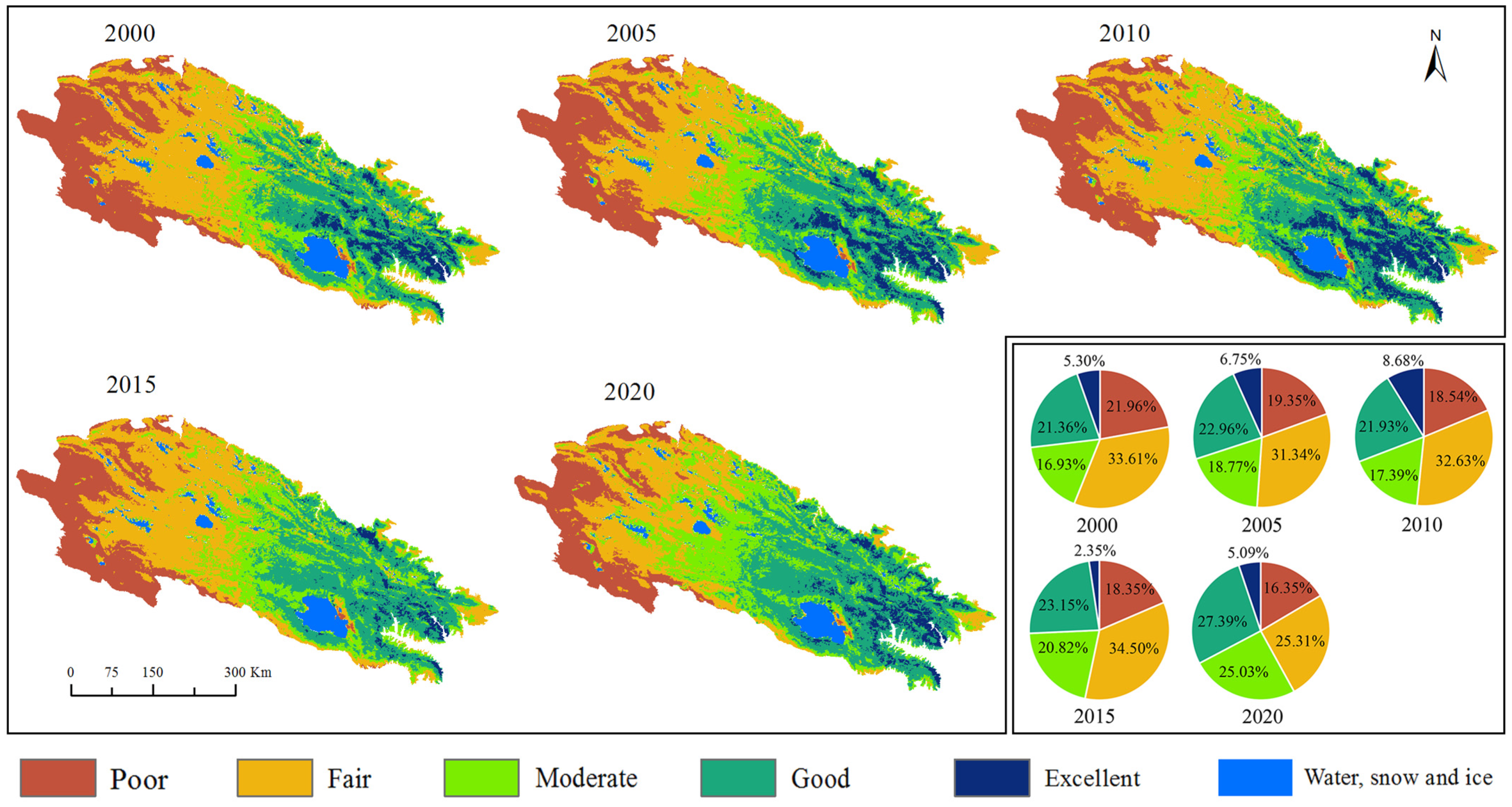
3.1. Spatiotemporal Distribution of EEQ

The SPCA results of the four ecological indicators and the mean RSEI values from 2000 to 2020 are shown in

Table 4. SPCA and the mean values of RSEI from 2000 to 2020.

Year	Item	PC1	PC2	PC3	PC4	RSEI ± SD
2000	Eigenvalue	0.042	0.009	0.002	0.001	0.408 ± 0.237
	Contribution rate (%)	78.907	16.916	3.119	1.059
2005	Eigenvalue	0.044	0.010	0.002	0.001	0.432 ± 0.240
	Contribution rate (%)	77.729	17.599	3.594	1.079
2010	Eigenvalue	0.044	0.009	0.002	0.001	0.438 ± 0.244
	Contribution rate (%)	79.115	16.070	3.505	1.309
2015	Eigenvalue	0.036	0.009	0.002	0.000	0.413 ± 0.219
	Contribution rate (%)	75.466	19.721	3.976	0.837
2020	Eigenvalue	0.033	0.010	0.002	0.000	0.460 ± 0.229
	Contribution rate (%)	74.243	21.307	3.597	0.853

Note: PC1, PC2, PC3, and PC4—the first, second, third, and fourth principal component, respectively; SD—standard deviation.

. PC1 has the largest eigenvalue, with a contribution rate exceeding 74% from 2000 to 2020 and a maximum contribution rate in 2010 (79.115%). Thus, PC1 can provide the most information regarding these indicators and is used to construct the RSEI in this study. The mean RSEI values range from 0.408 (2000) to 0.460 (2020), indicating an overall EEQ growth trend in the QLM during the study period, implying a gradual improvement in the area’s eco-environment. Specifically, the RSEI increases from 0.408 in 2000 to 0.438 in 2010; it then decreases to 0.413 in 2015 before increasing to 0.460 in 2020. Thus, the EEQ in the QLM first slightly improved (2000–2010), then deteriorated (2010–2015), and finally gradually recovered (2015–2020).

The spatial distribution of EEQ in the QLM from 2000 to 2020 indicates an increasing trend from northwest to southeast (Figure 4). Concretely speaking, the poor and fair EEQ levels are mostly recorded in the northwestern QLM (Dahaletenghe, Danghe, Shulehe, Da Qaidam Lake, and Hala Lake watersheds) due to the presence of bare land, low temperature, and rare precipitation. Moderate EEQ levels are recorded in the central part of the QLM region. The good and excellent EEQ levels are mainly clustered in the southeast of the area (Heihe, Datonghe, Shiyanghe, and Qinghai Lake watersheds), which is characterized by low elevation, relatively abundant precipitation, and high levels of vegetation coverage. Considering the fractions of different EEQ levels in the study area, excellent EEQ levels cover the least area (9%, Figure 4). The proportion of poor EEQ levels declined continuously from 2000 to 2020, but the moderate and good levels show fluctuating increase trends. In general, the EEQ shows an increasing trend from 2000 to 2020 in the QLM.

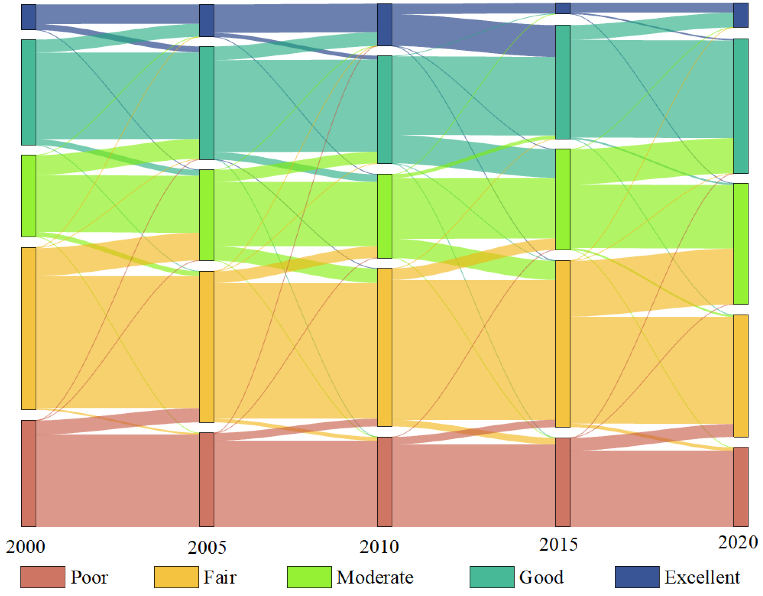
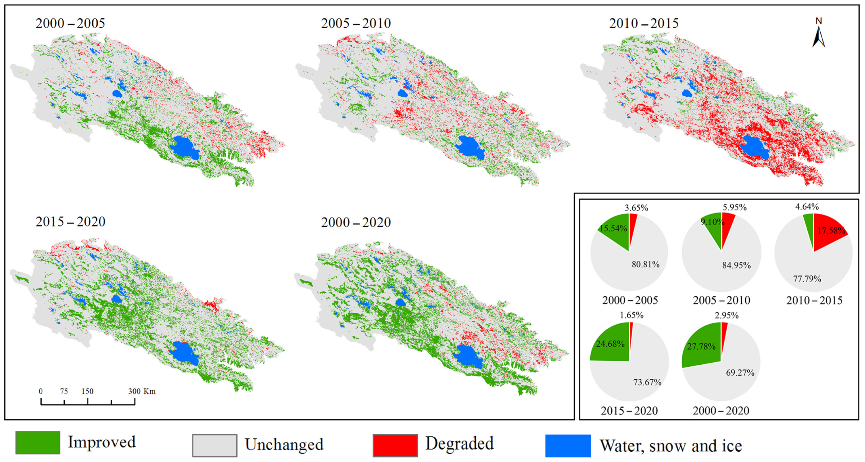
3.2. Dynamic Changes in EEQ from 2000 to 2020

To observe EEQ changes at each ecological level, we use a transition matrix to express detailed EEQ change processes from 2000 to 2020. Throughout the studied period, the EEQ is mainly at poor, fair, moderate, or good levels (Figure 5). Specifically, from 2000 to 2010, the EEQ shows an upward trend: the area of poor and fair levels decreased, and the area of good and excellent levels increased, with EEQ level transitions mostly from poor, fair, moderate, and good to fair, moderate, good, and excellent, respectively. During 2010–2015, the EEQ begins to deteriorate. The area of excellent EEQ level decreases significantly, while increasing trends are recorded for the areas of good, moderate, and fair levels (Figure 5). The EEQ shows an improved trend from 2015 to 2020, with a decrease in the area of poor and fair levels, with most EEQ transitions recorded from fair, moderate, and good levels to moderate, good, and excellent, respectively (Figure 5).

We use a spatial analysis method to study the EEQ spatiotemporal changes in different periods from 2000 to 2020 (Figure 6) based on the transition matrix in Table 2. During 2000–2015, the area of unchanged and improved EEQ decreased. However, the area of degraded EEQ increased, that was especially prominent in 2010–2015 when the area of improved EEQ was much less than that of degraded EEQ. After 2015, the area of unchanged EEQ continued to decrease. However, the area of improved EEQ is much greater than that of degraded EEQ, indicating that ecological deterioration in this period had largely been controlled. For example, during 2000–2005, the improved EEQ area was mainly concentrated around Qinghai Lake, while the area of degraded EEQ was distributed in the north of the area (Figure 6). However, from 2005 to 2015, the EEQ gradually degraded, with changes mainly concentrated in the southeastern QLM (Xichuanhe, Baokuhe, Datonghe, and Qinghai Lake watersheds). In contrast, in 2015–2020, the EEQ gradually improved; improved EEQ areas accounted for 24.68% of the total study area during this period, with improvements mainly concentrated around Hala Lake (Figure 6). In summary, from 2000 to 2020, the eco-environment of the QLM shows a trend of initial deterioration followed by improvement.

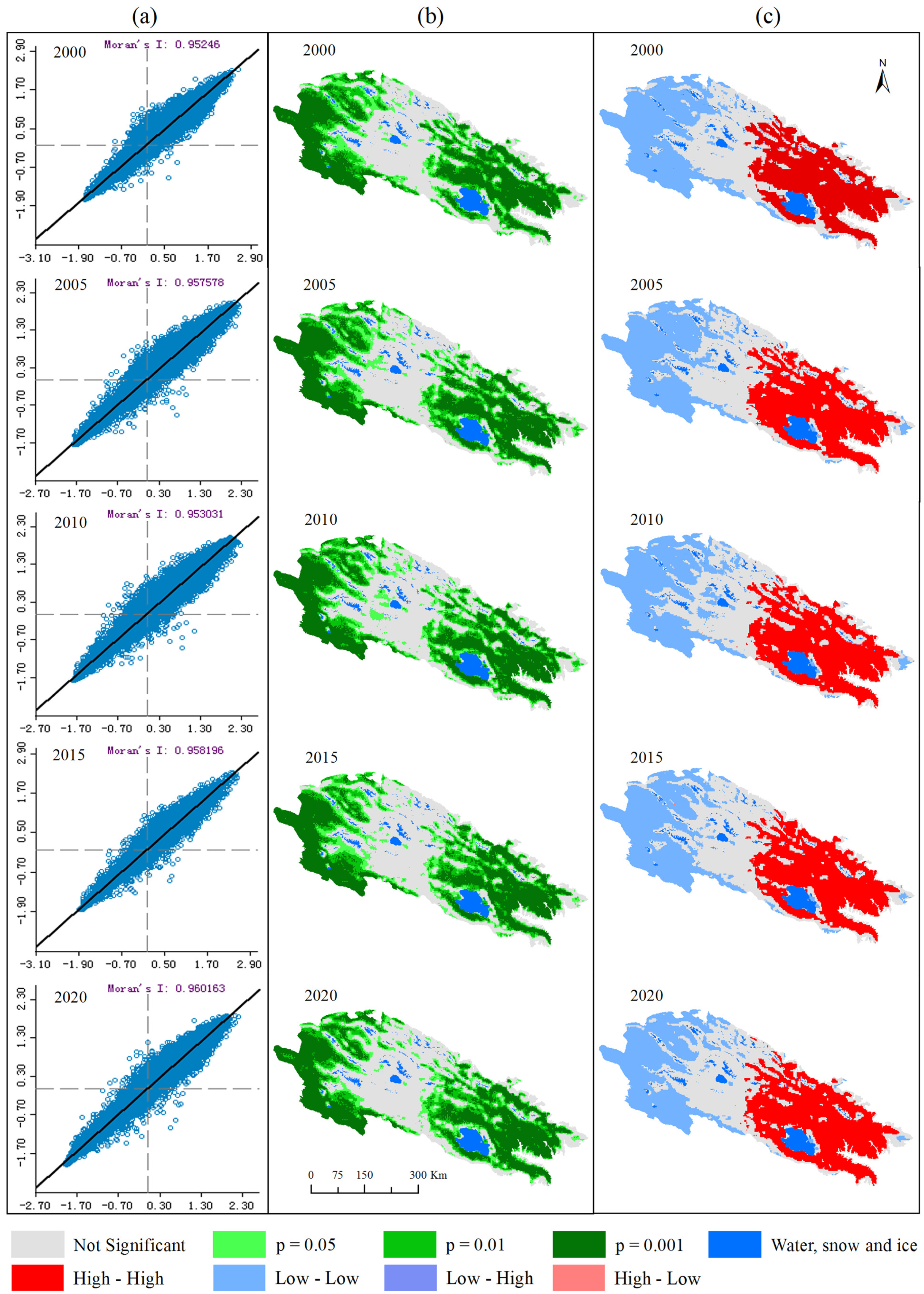
3.3. Spatial Autocorrelation Pattern of EEQ

To analyze the spatial autocorrelation of RSEI in the QLM from 2000 to 2020, the Moran’s I values, significance map, and LISA clustering map are used (Figure 7). The Moran’s I value remained between 0.95 and 0.96 from 2000 to 2020, indicating that the spatial distribution of EEQ in the QLM is highly positively spatially aggregated (Figure 7a). From the significance map, the insignificant area is mainly distributed in the central QLM (Hala Lake), implying that the environmental conditions are complex in this area (Figure 7b). In Figure 7c, at the 95% confidence level, “H-H” clusters are widely distributed in the southeast (Heihe, Babaohe, Datonghe, Xichuanhe, and Qinghai Lake watersheds). In contrast, the “L-L” clusters are concentrated in the northwest. Thus, the eco-environment of the QLM is polarized: the EEQ is low in the northwest while it is high in the southeast, potentially due to homogeneity in the main influencing factors.

3.4. Analysis of the Influencing Factors Based on Spatial Differences in RSEI

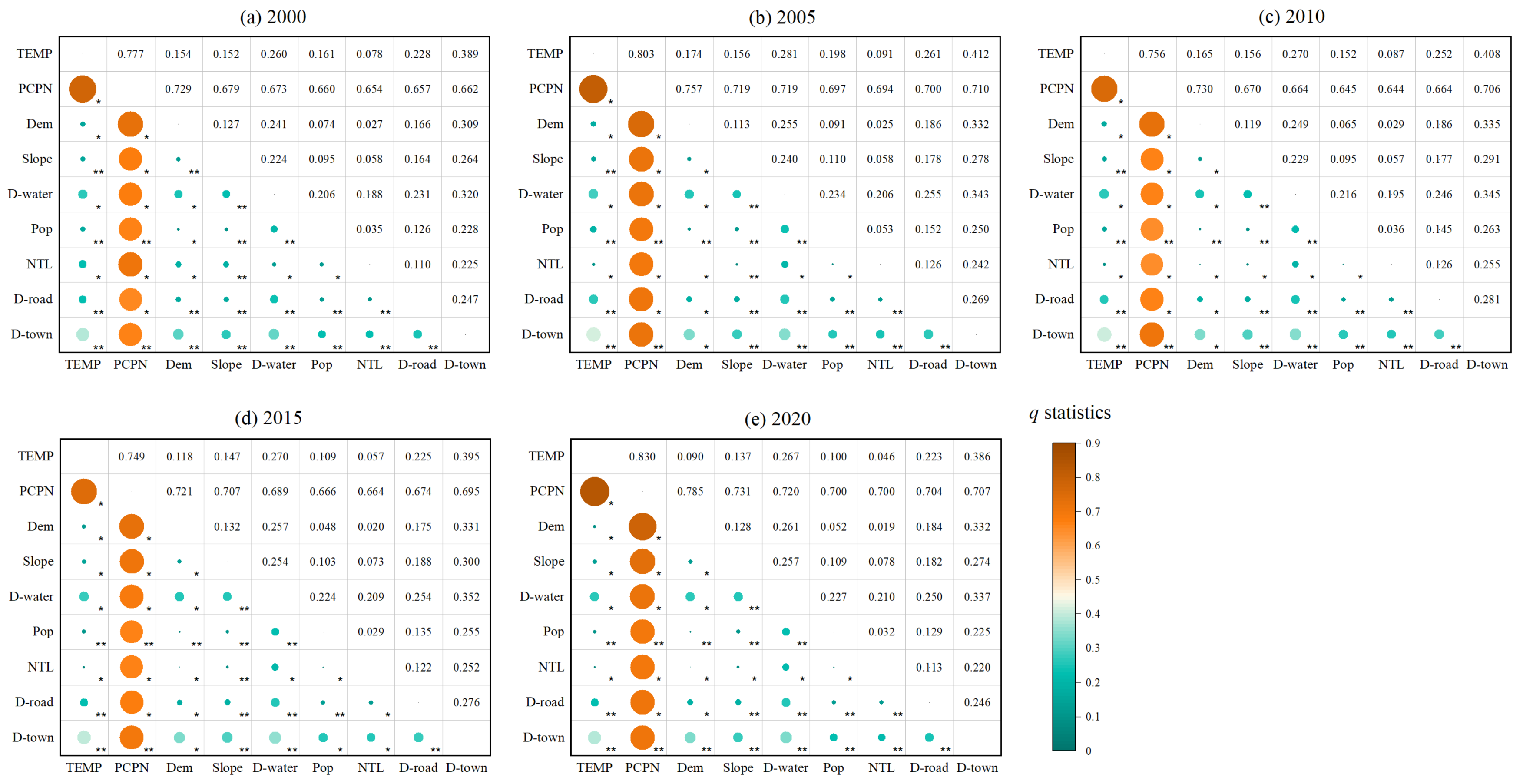
3.4.1. Analysis of Geographical Detector Results

The GeoDetector approach is used to calculate the individual and interaction effects of EEQ influencing factors (

Table 5. The q-statistics of factor detection.

Factor Type		2000	2005	2010	2015	2020
Natural factors	TEMP	0.078 **	0.090 **	0.086 **	0.057 **	0.042 **
	PCPN	0.654 **	0.693 **	0.644 **	0.664 **	0.699 **
	Dem	0.027 **	0.024 **	0.028 **	0.020 **	0.016 **
	Slope	0.058 **	0.057 **	0.056 **	0.072 **	0.075 **
	D-water	0.188 **	0.205 **	0.194 **	0.209 **	0.208 **
Human factors	Pop	0.035 **	0.052 **	0.035 **	0.027 **	0.031 **
	NTL	0.000	0.001	0.001	0.001	0.002
	D-road	0.110 **	0.126 **	0.125 **	0.121 **	0.112 **
	D-town	0.224 **	0.242 **	0.255 **	0.251 **	0.219 **

Note: ** p < 0.01.

and Figure 8). The q-statistics values, in order from high to low, are: PCPN > D-town > D-water > D-road > Slope > TEMP > Pop >Dem > NTL (Table 5). From 2000 to 2020, all factors have significant impacts on EEQ (p < 0.01), except NTL, potentially due to the faint night light in the remote region. PCPN exerted the strongest influence on EEQ, with an explanatory power of more than 0.644 during the study period. The D-town is the second most important factor with an explanatory power of more than 0.219, followed by D-water with q-statistics between 0.188 and 0.209. The remaining factors all had significant impacts on the EEQ but relatively low q-statistics (Table 5).

The results of interaction detection of influencing factor pairs on the EEQ of the QLM are illustrated in Figure 8. Overall, the explanatory powers (q-statistics values) of the interactions between factor pairs on EEQ are greater than those of any single factor. Specifically, the interaction between TEMP and PCPN is the greatest, with q-statistics values between 0.749 and 0.830 from 2000 to 2020 (Figure 8). The interactions between PCPN and other factors showed, q-statistics values between 0.644 and 0.785 with a bivariate enhancement interaction type, except for PCPN ∩ Dem. Furthermore, the q-statistics values of D-town and D-water with other driving factors range from 0.188 to 0.408. However, the interactions between NTL and other factors are the smallest (<0.087), except for NTL ∩ PCPN.

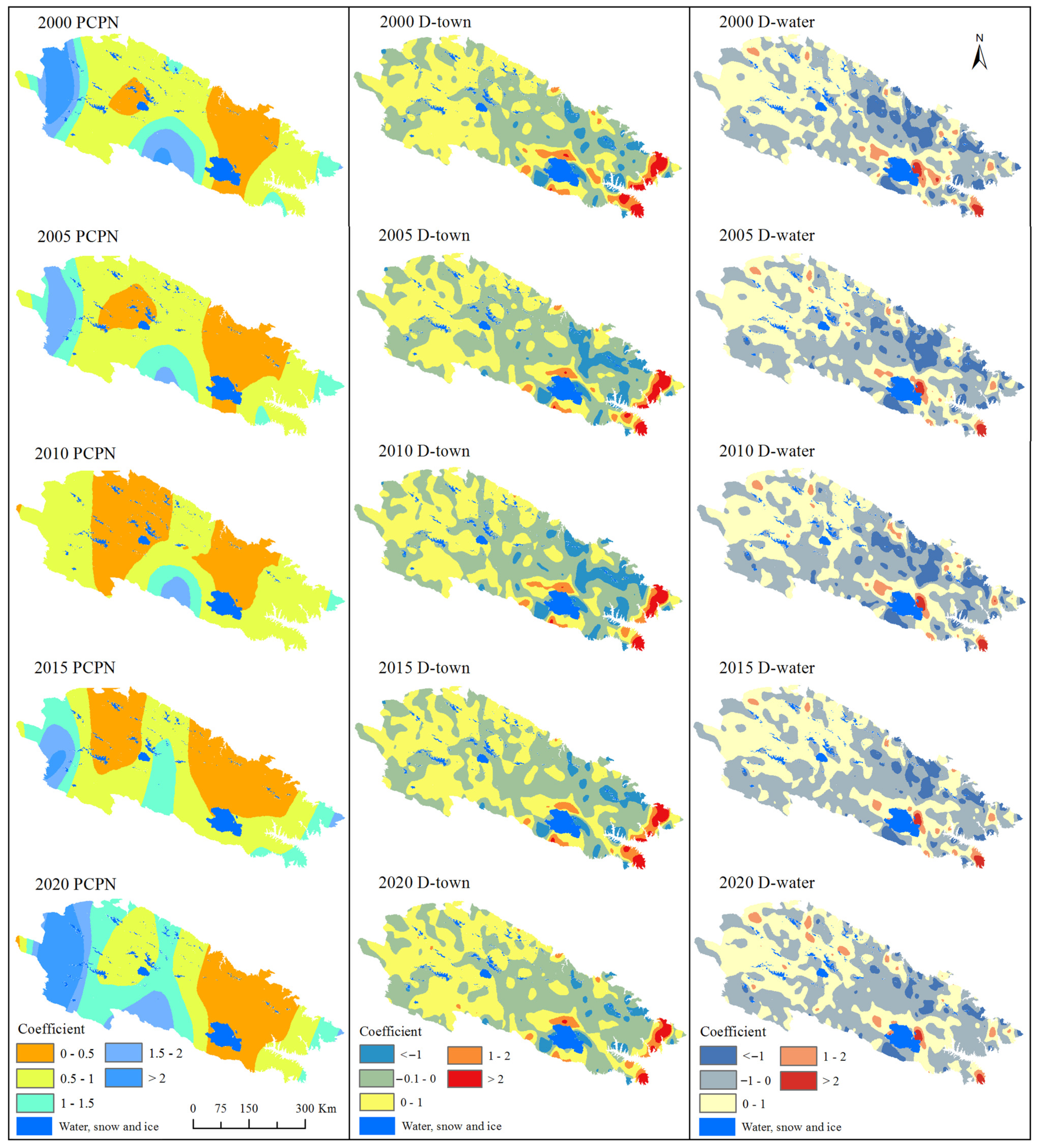
3.4.2. Spatial Heterogeneity Analysis of Driving Factors

Based on the GeoDetector analysis results from 2000 to 2020, PCPN, D-town, and D-water are the three main factors influencing EEQ in the QLM (Table 5). Therefore, we use the GWR model to further explore the impact of these three factors on the spatial heterogeneity of EEQ in the QLM region. In the GWR model, regression coefficients are used to represent the spatial distributions of the impact intensity of the three factors on EEQ (Figure 9). The mean regression coefficients of PCPN in the five periods from 2000 to 2020 are 0.915, 0.769, 0.596, 0.709, and 1.138, suggesting that PCPN positively influences EEQ in the QLM. From the spatial distribution of regression coefficients, the influence of PCPN decreases from the northwest to the southeast, with the northwestern part of the study area and the western Qinghai Lake affected the most (Figure 9). The mean regression coefficients of D-town and D-water are small (−0.117–0.019) with both positive and negative values; thus, the impact of these two factors on EEQ is considered uncertain.

4. Discussion

4.1. Spatiotemporal Variations in EEQ in the QLM

Quantifying EEQ is essential for establishing eco-environmental protection measures. In general, the overall eco-environment of the QLM gradually improved during our studied period. Yang et al. [30] and Gao et al. [58] also recorded significant improvements in NDVI in the QLM, indicating improvements in the eco-environment. From 2000 to 2015, the eco-environment showed a slight improvement followed by a deterioration trend (Figure 6). This may be due to human activities, such as overexploitation of mineral resources, unsustainable use of water resources, extensive development of tourism, and overgrazing. All of these aspects may have caused severe damage to the eco-environment in the QLM [2]. In response, the government has issued extensive ecological rectification policies and plans since 2015. In October 2018, the Qilian Mountain National Park Administration was officially established. Regulations for managing the Qilian Mountain National Parks were implemented, which further strengthened the eco-environment protection efforts in the QLM [2]. From 2015 to 2020, the overall RSEI increased from 0.413 to 0.460 (Table 4), indicating a significant improvement in the EEQ of the QLM. Furthermore, according to a recent report, eco-environment restoration of the QLM has achieved remarkable effects, with steady improvements in EEQ (http://sthj.gansu.gov.cn/sthj/c112982/202109/1795416.shtml, accessed on 30 December 2022), thus supporting our findings.

Based on the overall spatial distribution of EEQ in the QLM, the areas with high EEQ values were mainly concentrated in the southeast of the QLM from 2000 to 2020, with low EEQ values in the northwest of the area (Figure 4). The spatial distribution of EEQ is consistent with that of the area’s vegetation [59]. Areas with a fair ecological level are mainly covered by barren land, whereas those with good and excellent EEQ levels are covered by grassland, shrubland, and forest (Figure 1). In addition, the spatial distribution of the EEQ is consistent with the spatial distribution of precipitation in the QLM [59]. In general, in the southeastern part of the QLM, water resources are plentiful due to the impacts of monsoons, the temperature is suitable for plant growth, and vegetation coverage is high [29], leading to high RSEI values. Furthermore, our findings show that the EEQ was degraded from 2000 to 2015 but gradually improved from 2015 to 2020 (Figure 6). This result may be attributed to the severe eco-environmental damage in pursuit of economic development from 2000 to 2015; however, the government has adopted active and effective ecological rectification measures since 2015 and reversed this trend.

Although the overall eco-environment of the QLM shows an improvement trend, there is still marked spatial heterogeneity (Figure 7). The global Moran’s I of the RSEI is greater than 0.95 with a high degree of spatial clustering from 2000 to 2020. The LISA cluster maps mainly show “H-H” and “L-L” clustering types, which may be due to differences in the area’s natural conditions. The spatial patterns of precipitation lead to low average NDVI values in the growing season in the northwest and high values in the southeast of the QLM [28,59]. Xu et al. [60] also found that the gross primary production of the QLM followed a similar spatial distribution.

4.2. Dominant Factors Affecting EEQ

Identifying the main factors influencing EEQ changes can provide a helpful reference for policymakers. In the present study, the GeoDetector results demonstrate that PCPN is the dominant factor affecting EEQ in the QLM. This may be due to the location of the QLM and the effect of monsoons and the westerlies. These factors lead to spatial differences in precipitation which, in turn, affect the spatial distribution of the vegetation [61]. Therefore, they predetermine the spatial distribution of EEQ. Teng et al. [62] and Sun et al. [63] also found that precipitation is the main factor affecting changes in net primary productivity and vegetation phenology in the QLM. In addition, our GWR analysis results show that PCPN has a positive effect on EEQ in the QLM, which is in agreement with Gao et al. [58]. Other natural factors also have a significant impact on EEQ. The influences of D-water, TEMP, Slope, and Dem decrease progressively, with mean q-values of 0.201, 0.071, 0.064, and 0.023, respectively (Table 5). The effects of D-water on EEQ may be related to the spatial distribution of rivers and lakes. The EEQ is less sensitive to TEMP than PCPN because the QLM region is characterized by low temperatures. The low q-values of Slope and Dem indicate that topographic factors have minimal effects on the EEQ.

In comparison with natural factors, human factors have less impact on EEQ throughout the study area. Among these, D-town is the most significant human factor influencing EEQ in the QLM, followed by D-road. In contrast, Pop and NTL have relatively little impact on the EEQ, which may be due to the low population density and low development level of the QLM (Figure 2e,f). Temporal changes in EEQ are closely related to the strong support of effective measures by relevant national and local government departments. Our results show that the overall EEQ of the QLM improved from 2000 to 2020, especially after 2015, because the Gansu and Qinghai Provinces issued a series of policies and plans to rectify and improve the eco-environment of the QLM. Li et al. [2] note that the government departments of the Gansu Province issued 543 planning documents relating to the QLM. Additionally, the central and provincial governments have invested 19.5 billion yuan in special funds for ecological protection to support eco-environment restoration in the QLM since 2017 (http://sthj.gansu.gov.cn/sthj/c112982/202109/1795416.shtml, accessed on 30 December 2022). The establishment of Qilian Mountain National Park was essential for the area’s EEQ through promoting relevant system management specifications and further strengthening eco-environment protection in the QLM.

The EEQ changes identified in this work were not determined by an individual influencing factor, and the interactions between independent factors on EEQ play an important role. Our findings show that the interaction between TEMP and PCPN exerts the largest influence on EEQ (Figure 8). Temperature and precipitation are stress factors that inhibit vegetation growth [32]; thus the interaction of these two factors will inevitably have a significant impact on EEQ changes. We also identified relatively large interactive q-statistics value for PCPN and other factors, indicating that PCPN is the main factor driving EEQ changes in the QLM. In summary, PCPN is the leading natural factor impacting the spatial variation of EEQ, and the interaction impacts of PCPN with other factors are greater than those of PCPN itself, consistent with the findings of Wu et al. [64]. In addition, policy support is identified as the primary human factor impacting temporal trends in EEQ changes.

4.3. Uncertainty and Prospects

This study adopts the RSEI proposed by Xu [14] to comprehensively reflect the ecological status of the QLM and analyze its EEQ. Compared to other single eco-environmental indexes, RSEI employs the SPCA method to integrate four important indicators closely related to EEQ, which can more objectively reflect regional eco-environmental conditions [44]. Shan et al. [65] compared the EI and RSEI and found that RSEI can reasonably and effectively reflect the regional EEQ status. However, the RSEI is primarily used to monitor the ecological state of urban areas [45], and has been gradually used to evaluate the EEQ of basins and wetlands [9,12]. Similar to other studies, there are still some uncertainties in the current work. First, in the QLM, which is characterized by complex terrain, only four indicators are used to reflect the structure and function of the ecosystem, which cannot comprehensively describe the area’s ecological conditions. Second, the road, town, and water data used in the study are limited to one period. In future studies, if data for these aspects could be obtained for different periods, the driving mechanisms of EEQ in the QLM over time could be explored in more depth. Third, although MODIS image data have good quality and a short revisit period, they have a low spatial resolution; thus, higher resolution multi-source remote sensing data should be considered in the future. Overall, despite these limitations, the results of this research can assist researchers and policymakers in understanding the change trends and influencing factors of EEQ in the QLM and can offer a scientific basis for eco-environmental protection and restoration in the region.

5. Conclusions

In summary, we use the RSEI to monitor spatiotemporal changes in EEQ in the QLM from 2000 to 2020 and quantitatively explore the factors influencing EEQ by combining GeoDetector and GWR models. Spatially, the EEQ increases from northwest to southeast; temporally, the EEQ initially slightly improved, then deteriorated, and finally gradually recovered from 2000 to 2020. The explanatory power of the driving factors for EEQ from high to low are: PCPN > D-town > D-water > D-road > Slope > TEMP > Pop >Dem > NTL. Natural factors mainly control the spatial patterns of the EEQ, represented as “H-H” clusters in the southeast and “L-L” clusters in the northwest, which are primarily influenced by precipitation. Human factors have an important impact on temporal EEQ trends in the QLM, with significant EEQ improvements recorded since 2015, which are closely linked to the implementation of effective measures by relevant government departments. Overall, our results help to fill a current research gap in the assessment of EEQ in the QLM and can provide a new research perspective to understand eco-environment sustainable development in arid and semi-arid regions.

References

1. Qin, X.; Liu, W.B.; Mao, R.C.; Song, J.X.; Chen, Y.N.; Ma, C.; Li, M.Y. Quantitative assessment of driving factors affecting human appropriation of net primary production (HANPP) in the Qilian Mountains, China. Ecol. Indic. 2021, 121, 106997. [Google Scholar] [CrossRef]
2. Li, Z.X.; Qi, F.; Li, Z.J.; Wang, X.F.; Juan, G.; Zhang, B.J.; Li, Y.C.; Deng, X.H.; Jian, X.; Gao, W.D.; et al. Reversing conflict between humans and the environment-The experience in the Qilian Mountains. Renew. Sustain. Energy Rev. 2021, 148, 111333. [Google Scholar] [CrossRef]
3. Yao, Z.Y.; Zhao, C.Y.; Yang, K.S.; Liu, W.C.; Li, Y.; You, J.D.; Xiao, J.H. Alpine grassland degradation in the Qilian Mountains, China-A case study in Damaying Grassland. CATENA 2016, 137, 494–500. [Google Scholar] [CrossRef]
4. Zhu, Q.; Guo, J.X.; Guo, X.; Chen, L.; Han, Y.; Liu, S.Y. Relationship between ecological quality and ecosystem services in a red soil hilly watershed in southern China. Ecol. Indic. 2021, 121, 107119. [Google Scholar] [CrossRef]
5. Yue, H.; Liu, Y.; Li, Y.; Lu, Y. Eco-Environmental Quality Assessment in China’s 35 Major Cities Based on Remote Sensing Ecological Index. IEEE Access 2019, 7, 51295–51311. [Google Scholar] [CrossRef]
6. Willis, K.S. Remote sensing change detection for ecological monitoring in United States protected areas. Biol. Conserv. 2015, 182, 233–242. [Google Scholar] [CrossRef]
7. Liu, C.L.; Li, W.L.; Wang, W.Y.; Zhou, H.K.; Liang, T.G.; Hou, F.J.; Xu, J.; Xue, P.F. Quantitative spatial analysis of vegetation dynamics and potential driving factors in a typical alpine region on the northeastern Tibetan Plateau using the Google Earth Engine. Catena 2021, 206, 105500. [Google Scholar] [CrossRef]
8. Xu, H.Q.; Wang, Y.F.; Guan, H.D.; Shi, T.T.; Hu, X.S. Detecting Ecological Changes with a Remote Sensing Based Ecological Index (RSEI) Produced Time Series and Change Vector Analysis. Remote Sens. 2019, 11, 2345. [Google Scholar] [CrossRef]
9. Xiong, Y.; Xu, W.H.; Lu, N.; Huang, S.D.; Wu, C.; Wang, L.G.; Dai, F.; Kou, W.L. Assessment of spatial? Temporal changes of ecological environment quality based on RSEI and GEE: A case study in Erhai Lake Basin, Yunnan province, China. Ecol. Indic. 2021, 125, 107518. [Google Scholar] [CrossRef]
10. Xu, H.Q.; Wang, M.Y.; Shi, T.T.; Guan, H.D.; Fang, C.Y.; Lin, Z.L. Prediction of ecological effects of potential population and impervious surface increases using a remote sensing based ecological index (RSEI). Ecol. Indic. 2018, 93, 730–740. [Google Scholar] [CrossRef]
11. Liao, W.H.; Jiang, W.G. Evaluation of the Spatiotemporal Variations in the Eco-environmental Quality in China Based on the Remote Sensing Ecological Index. Remote Sens. 2020, 12, 2462. [Google Scholar] [CrossRef]
12. Jing, Y.Q.; Zhang, F.; He, Y.F.; Kung, H.T.; Johnson, V.C.; Arikena, M. Assessment of spatial and temporal variation of ecological environment quality in Ebinur Lake Wetland National Nature Reserve, Xinjiang, China. Ecol. Indic. 2020, 110, 105874. [Google Scholar] [CrossRef]
13. Liu, Y.X.; Liu, S.L.; Sun, Y.X.; Li, M.Q.; An, Y.; Shi, F.N. Spatial differentiation of the NPP and NDVI and its influencing factors vary with grassland type on the Qinghai-Tibet Plateau. Environ. Monit. Assess. 2021, 193, 48. [Google Scholar] [CrossRef]
14. Xu, H. A remote sensing index for assessment of regional ecological changes. China Environ. Sci. 2013, 33, 889–897. [Google Scholar]
15. Hu, X.S.; Xu, H.Q. A new remote sensing index for assessing the spatial heterogeneity in urban ecological quality: A case from Fuzhou City, China. Ecol. Indic. 2018, 89, 11–21. [Google Scholar] [CrossRef]
16. Zheng, Z.H.; Wu, Z.F.; Chen, Y.B.; Yang, Z.W.; Marinello, F. Exploration of eco-environment and urbanization changes in coastal zones: A case study in China over the past 20 years. Ecol. Indic. 2020, 119, 106847. [Google Scholar] [CrossRef]
17. Bi, X.; Chang, B.R.; Hou, F.; Yang, Z.H.; Fu, Q.; Li, B. Assessment of Spatio-Temporal Variation and Driving Mechanism of Ecological Environment Quality in the Arid Regions of Central Asia, Xinjiang. Int. J. Environ. Res. Public Health 2021, 18, 7111. [Google Scholar] [CrossRef]
18. Guo, B.B.; Fang, Y.L.; Jin, X.B.; Zhou, Y.K. Monitoring the effects of land consolidation on the ecological environmental quality based on remote sensing: A case study of Chaohu Lake Basin, China. Land Use Policy 2020, 95, 104569. [Google Scholar] [CrossRef]
19. Yuan, B.D.; Fu, L.N.; Zou, Y.; Zhang, S.Q.; Chen, X.S.; Li, F.; Deng, Z.M.; Xie, Y.H. Spatiotemporal change detection of ecological quality and the associated affecting factors in Dongting Lake Basin, based on RSEI. J. Clean. Prod. 2021, 302, 126995. [Google Scholar] [CrossRef]
20. Boori, M.S.; Choudhary, K.; Paringer, R.; Kupriyanov, A. Eco-environmental quality assessment based on pressure-state-response framework by remote sensing and GIS. Remote Sens. Appl. Soc. Environ. 2021, 23, 100530. [Google Scholar] [CrossRef]
21. Wang, Y.Z.; Yu, K.F.; Chen, X.Y.; Wang, W.H.; Huang, X.Y.; Wang, Y.H.; Liao, Z.H. An approach for assessing ecosystem-based adaptation in coral reefs at relatively high latitudes to climate change and human pressure. Environ. Monit. Assess. 2020, 192, 579. [Google Scholar] [CrossRef] [PubMed]
22. Bagan, H.; Yamagata, Y. Analysis of urban growth and estimating population density using satellite images of nighttime lights and land-use and population data. GISci. Remote Sens. 2015, 52, 765–780. [Google Scholar] [CrossRef]
23. Wang, J.F.; Li, X.H.; Christakos, G.; Liao, Y.L.; Zhang, T.; Gu, X.; Zheng, X.Y. Geographical Detectors-Based Health Risk Assessment and its Application in the Neural Tube Defects Study of the Heshun Region, China. Int. J. Geogr. Inf. Sci. 2010, 24, 107–127. [Google Scholar] [CrossRef]
24. Wang, H.; Liu, L.B.; Yin, L.; Shen, J.S.; Li, S.C. Exploring the complex relationships and drivers of ecosystem services across different geomorphological types in the Beijing-Tianjin-Hebei region, China (2000–2018). Ecol. Indic. 2021, 121, 107116. [Google Scholar] [CrossRef]
25. Xie, E.Z.; Zhang, Y.X.; Huang, B.; Zhao, Y.C.; Shi, X.Z.; Hu, W.Y.; Qu, M.K. Spatiotemporal variations in soil organic carbon and their drivers in southeastern China during 1981–2011. Soil Tillage Res. 2021, 205, 104763. [Google Scholar] [CrossRef]
26. Zhang, Z.Y.; Liu, Y.F.; Wang, Y.H.; Liu, Y.L.; Zhang, Y.; Zhang, Y. What factors affect the synergy and tradeoff between ecosystem services, and how, from a geospatial perspective? J. Clean. Prod. 2020, 257, 120454. [Google Scholar] [CrossRef]
27. Xu, H.J.; Zhao, C.Y.; Wang, X.P. Elevational differences in the net primary productivity response to climate constraints in a dryland mountain ecosystem of northwestern China. Land Degrad. Dev. 2020, 31, 2087–2103. [Google Scholar] [CrossRef]
28. Geng, L.Y.; Che, T.; Wang, X.F.; Wang, H.B. Detecting Spatiotemporal Changes in Vegetation with the BFAST Model in the Qilian Mountain Region during 2000–2017. Remote Sens. 2019, 11, 103. [Google Scholar] [CrossRef]
29. Wang, H.; Liu, C.L.; Zang, F.; Yang, J.H.; Li, N.; Rong, Z.L.; Zhao, C.Y. Impacts of Topography on the Land Cover Classification in the Qilian Mountains, Northwest China. Can. J. Remote Sens. 2020, 46, 344–359. [Google Scholar] [CrossRef]
30. Yang, L.S.; Feng, Q.; Adamowski, J.F.; Alizadeh, M.R.; Yin, Z.L.; Wen, X.H.; Zhu, M. The role of climate change and vegetation greening on the variation of terrestrial evapotranspiration in northwest China’s Qilian Mountains. Sci. Total Environ. 2021, 759, 143532. [Google Scholar] [CrossRef]
31. Lu, J.Z.; Lu, H.W.; Brusseau, M.L.; He, L.; Gorlier, A.; Yao, T.C.; Tian, P.P.; Feng, S.S.; Yu, Q.; Nie, Q.W.; et al. Interaction of climate change, potentially toxic elements (PTEs), and topography on plant diversity and ecosystem functions in a high-altitude mountainous region of the Tibetan Plateau. Chemosphere 2021, 275, 130099. [Google Scholar] [CrossRef]
32. Chen, L.F.; Zhang, H.; Zhang, X.Y.; Liu, P.H.; Zhang, W.C.; Ma, X.Y. Vegetation changes in coal mining areas: Naturally or anthropogenically Driven? CATENA 2022, 208, 105712. [Google Scholar] [CrossRef]
33. Feng, R.D.; Wang, F.Y.; Wang, K.Y.; Wang, H.J.; Li, L. Urban ecological land and natural-anthropogenic environment interactively drive surface urban heat island: An urban agglomeration-level study in China. Environ. Int. 2021, 157, 106857. [Google Scholar] [CrossRef]
34. Wang, H.; Zang, F.; Zhao, C.Y.; Liu, C.L. A GWR downscaling method to reconstruct high-resolution precipitation dataset based on GSMaP-Gauge data: A case study in the Qilian Mountains, Northwest China. Sci. Total Environ. 2022, 810, 152066. [Google Scholar] [CrossRef]
35. Chen, Z.Q.; Yu, B.L.; Yang, C.S.; Zhou, Y.Y.; Yao, S.J.; Qian, X.J.; Wang, C.X.; Wu, B.; Wu, J.P. An extended time series (2000-2018) of global NPP-VIIRS-like nighttime light data from a cross-sensor calibration. Earth Syst. Sci. Data 2021, 13, 889–906. [Google Scholar] [CrossRef]
36. Boori, M.S.; Choudhary, K.; Paringer, R.; Kupriyanov, A. Spatiotemporal ecological vulnerability analysis with statistical correlation based on satellite remote sensing in Samara, Russia. J. Environ. Manag. 2021, 285, 112138. [Google Scholar] [CrossRef]
37. Healey, S.P.; Cohen, W.B.; Yang, Z.Q.; Krankina, O.N. Comparison of Tasseled Cap-based Landsat data structures for use in forest disturbance detection. Remote Sens. Environ. 2005, 97, 301–310. [Google Scholar] [CrossRef]
38. Xu, H. A new index for delineating built-up land features in satellite imagery. Int. J. Remote Sens. 2008, 29, 4269–4276. [Google Scholar] [CrossRef]
39. Weng, Q.H.; Fu, P.; Gao, F. Generating daily land surface temperature at Landsat resolution by fusing Landsat and MODIS data. Remote Sens. Environ. 2014, 145, 55–67. [Google Scholar] [CrossRef]
40. Khodaparast, M.; Rajabi, A.M.; Edalat, A. Municipal solid waste landfill siting by using GIS and analytical hierarchy process (AHP): A case study in Qom city, Iran. Environ. Earth Sci. 2018, 77, 52. [Google Scholar] [CrossRef]
41. Abson, D.J.; Dougill, A.J.; Stringer, L.C. Using Principal Component Analysis for information-rich socio-ecological vulnerability mapping in Southern Africa. Appl. Geogr. 2012, 35, 515–524. [Google Scholar] [CrossRef]
42. Li, W.L.; Liu, C.L.; Su, W.L.; Ma, X.L.; Zhou, H.K.; Wang, W.Y.; Zhu, G.F. Spatiotemporal evaluation of alpine pastoral ecosystem health by using the Basic-Pressure-State-Response Framework: A case study of the Gannan region, northwest China. Ecol. Indic. 2021, 129, 108000. [Google Scholar] [CrossRef]
43. Chen, J.B.; Wang, Y.J.; Li, F.Y.; Liu, Z.C. Aquatic ecosystem health assessment of a typical sub-basin of the Liao River based on entropy weights and a fuzzy comprehensive evaluation method. Sci. Rep. 2019, 9, 14045. [Google Scholar] [CrossRef] [PubMed]
44. Ariken, M.; Zhang, F.; Liu, K.; Fang, C.L.; Kung, H.T. Coupling coordination analysis of urbanization and eco-environment in Yanqi Basin based on multi-source remote sensing data. Ecol. Indic. 2020, 114, 106331. [Google Scholar] [CrossRef]
45. Yang, C.; Zhang, C.C.; Li, Q.Q.; Liu, H.Z.; Gao, W.X.; Shi, T.Z.; Liu, X.; Wu, G.F. Rapid urbanization and policy variation greatly drive ecological quality evolution in Guangdong-Hong Kong-Macau Greater Bay Area of China: A remote sensing perspective. Ecol. Indic. 2020, 115, 106373. [Google Scholar] [CrossRef]
46. Darand, M.; Dostkamyan, M.; Rehmanic, M.I.A. Spatial Autocorrelation Analysis of Extreme Precipitation in Iran. Russ. Meteorol. Hydrol. 2017, 42, 415–424. [Google Scholar] [CrossRef]
47. Moran, P.A.P. Notes on continuous stochastic phenomena. Biometrika 1950, 37, 17–23. [Google Scholar] [CrossRef]
48. Ghulam, A.; Ghulam, O.; Maimaitijiang, M.; Freeman, K.; Porton, I.; Maimaitiyiming, M. Remote Sensing Based Spatial Statistics to Document Tropical Rainforest Transition Pathways. Remote Sens. 2015, 7, 6257–6279. [Google Scholar] [CrossRef]
49. Anselin, L.; Syabri, I.; Kho, Y. GeoDa: An introduction to spatial data analysis. Geogr. Anal. 2006, 38, 5–22. [Google Scholar] [CrossRef]
50. Wang, H.; Liu, X.M.; Zhao, C.Y.; Chang, Y.P.; Liu, Y.Y.; Zang, F. Spatial-temporal pattern analysis of landscape ecological risk assessment based on land use/land cover change in Baishuijiang National nature reserve in Gansu Province, China. Ecol. Indic. 2021, 124, 107454. [Google Scholar] [CrossRef]
51. Song, Y.Z.; Wang, J.F.; Ge, Y.; Xu, C.D. An optimal parameters-based geographical detector model enhances geographic characteristics of explanatory variables for spatial heterogeneity analysis: Cases with different types of spatial data. GISci. Remote Sens. 2020, 57, 593–610. [Google Scholar] [CrossRef]
52. Brunsdon, C.; Fotheringham, A.S.; Charlton, M.E. Geographically Weighted Regression: A Method for Exploring Spatial Nonstationarity. Geogr. Anal. 1996, 28, 281–298. [Google Scholar] [CrossRef]
53. Hou, W.J.; Gao, J.B. Spatially Variable Relationships between Karst Landscape Pattern and Vegetation Activities. Remote Sens. 2020, 12, 1134. [Google Scholar] [CrossRef]
54. Lu, B.B.; Charlton, M.; Harris, P.; Fotheringham, A.S. Geographically weighted regression with a non- Euclidean distance metric: A case study using hedonic house price data. Int. J. Geogr. Inf. Sci. 2014, 28, 660–681. [Google Scholar] [CrossRef]
55. He, Y.H.; Tang, C.C.; Wang, Z.R. Spatial patterns and influencing factors of sewage treatment plants in the Guangdong-Hong Kong-Macau Greater Bay Area, China. Sci. Total Environ. 2021, 792, 148430. [Google Scholar] [CrossRef]
56. Lin, Y.Y.; Hu, X.S.; Zheng, X.X.; Hou, X.Y.; Zhang, Z.X.; Zhou, X.N.; Qiu, R.Z.; Lin, J.G. Spatial variations in the relationships between road network and landscape ecological risks in the highest forest coverage region of China. Ecol. Indic. 2019, 96, 392–403. [Google Scholar] [CrossRef]
57. Fang, L.L.; Wang, L.C.; Chen, W.X.; Sun, J.; Cao, Q.; Wang, S.Q.; Wang, L.Z. Identifying the impacts of natural and human factors on ecosystem service in the Yangtze and Yellow River Basins. J. Clean. Prod. 2021, 314, 127995. [Google Scholar] [CrossRef]
58. Gao, X.; Huang, X.X.; Lo, K.; Dang, Q.W.; Wen, R.Y. Vegetation responses to climate change in the Qilian Mountain Nature Reserve, Northwest China. Glob. Ecol. Conserv. 2021, 28, e01698. [Google Scholar] [CrossRef]
59. Ma, Y.R.; Guan, Q.Y.; Sun, Y.F.; Zhang, J.; Yang, L.Q.; Yang, E.Q.; Li, H.C.; Du, Q.Q. Three-dimensional dynamic characteristics of vegetation and its response to climatic factors in the Qilian Mountains. CATENA 2022, 208, 105694. [Google Scholar] [CrossRef]
60. Xu, H.J.; Zhao, C.Y.; Wang, X.P. Spatiotemporal differentiation of the terrestrial gross primary production response to climate constraints in a dryland mountain ecosystem of northwestern China. Agric. For. Meteorol. 2019, 276, 107628. [Google Scholar] [CrossRef]
61. Zhu, L.J.; Meng, J.J.; Zhu, L.K. Applying Geodetector to disentangle the contributions of natural and anthropogenic factors to NDVI variations in the middle reaches of the Heihe River Basin. Ecol. Indic. 2020, 117, 106545. [Google Scholar] [CrossRef]
62. Teng, M.J.; Zeng, L.X.; Hu, W.J.; Wang, P.C.; Yan, Z.G.; He, W.; Zhang, Y.; Huang, Z.L.; Xiao, W.F. The impacts of climate changes and human activities on net primary productivity vary across an ecotone zone in Northwest China. Sci. Total Environ. 2020, 714, 136691. [Google Scholar] [CrossRef] [PubMed]
63. Sun, Y.F.; Guan, Q.Y.; Wang, Q.Z.; Yang, L.Q.; Pan, N.H.; Ma, Y.R.; Luo, H.P. Quantitative assessment of the impact of climatic factors on phenological changes in the Qilian Mountains, China. For. Ecol. Manag. 2021, 499, 119594. [Google Scholar] [CrossRef]
64. Wu, H.W.; Guo, B.; Fan, J.F.; Yang, F.; Han, B.M.; Wei, C.X.; Lu, Y.F.; Zang, W.Q.; Zhen, X.Y.; Meng, C. A novel remote sensing ecological vulnerability index on large scale: A case study of the China-Pakistan Economic Corridor region. Ecol. Indic. 2021, 129, 107955. [Google Scholar] [CrossRef]
65. Shan, W.; Jin, X.B.; Ren, J.; Wang, Y.C.; Xu, Z.G.; Fan, Y.T.; Gu, Z.M.; Hong, C.Q.; Lin, J.H.; Zhou, Y.K. Ecological environment quality assessment based on remote sensing data for land consolidation. J. Clean. Prod. 2019, 239, 118126. [Google Scholar] [CrossRef]
Figure 1. The Location, Digital Elevation Model (DEM), and the spatial distribution of land cover in the QLM.
Remotesensing 15 00960 g001
Figure 2. The spatial distribution of nine driving factors in 2020.
Remotesensing 15 00960 g002
Figure 3. Flow diagram of the study.
Remotesensing 15 00960 g003
Figure 4. Spatial distribution and area ratio of different EEQ levels in the QLM from 2000 to 2020.
Remotesensing 15 00960 g004
Figure 5. The transition matrix of different EEQ levels in the QLM from 2000 to 2020.
Remotesensing 15 00960 g005
Figure 6. The spatiotemporal changes and area ratios of EEQ in the QLM from 2000 to 2020.
Remotesensing 15 00960 g006
Figure 7. The Moran scatter plots (a), significance maps (b), and LISA clustering maps (c) of EEQ in the QLM from 2000 to 2020.
Remotesensing 15 00960 g007
Figure 8. Interaction effects (q-statistics value) of the driving factors on EEQ in the QLM. * p < 0.05, ** p < 0.01.
Remotesensing 15 00960 g008
Figure 9. The spatial distribution of GWR regression coefficients of three main factors in 2000, 2005, 2010, 2015, and 2020.
Remotesensing 15 00960 g009