Article

Links between Land Cover and In-Water Optical Properties in Four Optically Contrasting Swedish Bays

1
Department of Ecology, Environment and Plant Sciences (DEEP), Stockholm University, 10691 Stockholm, Sweden
2
National Institute of Applied Sciences (INSA), 20 Av. Albert Einstein, 69100 Villeurbanne, France
*
Author to whom correspondence should be addressed.
Remote Sens. 2024, 16(1), 176; https://doi.org/10.3390/rs16010176
Submission received: 18 September 2023 / Revised: 27 October 2023 / Accepted: 23 December 2023 / Published: 31 December 2023
(This article belongs to the Special Issue Oceans from Space V)

Abstract

:
The optical complexity of coastal waters is mostly caused by the water discharged from land carrying optical components (such as dissolved and particulate matter) into coastal bays and estuaries, and increasing the attenuation of light. This paper aims to investigate the links between in-water optical properties in four Swedish bays (from the northern Baltic proper up to the Bothnian bay) and the land use and land cover (LULC) in the respective catchment of each bay. The optical properties were measured in situ over the last decade by various research and monitoring groups while the LULC in each bay was classified using the Copernicus Land Monitoring Service based on Landsat 8/OLI data. The absorption coefficient of colored dissolve organic matter (CDOM) at 440 nm, aCDOM (440), was significantly correlated to Wetlands which may act as sources of CDOM, while Developed areas (Agricultural and Urban classes) were negatively correlated. The Agriculture class was also negatively related to suspended particulate organic matter (SPOM), whilst Coniferous Forests and Mixed Forests as well as Meadows were positively correlated. SPOM seems thus to mostly originate from Natural classes, possibly due to the release of pollen and other organic matter. Overall, the methods applied here allow for a better understanding of effects of land use and land cover on the bio-optical properties, and thus coastal water quality, on a macroscopic scale.

1. Introduction

Seen from space, or from a plane, coastal waters are usually not blue but often yellow or brownish, or even green or red during certain phytoplankton blooms. The yellow-brown shades are mostly due to one of the main optical components often found in coastal waters: CDOM, also referred to as “yellow substance”. It consist of humic and fulvic substances [1] which have a complex chemical nature, consisting mostly of diverse polymers with aromatic rings and long chains of alkyls [2]. Humic substances are derived from the decomposition of plants and are ultimately drained into coasts by rivers and by runoff from land [1]. CDOM has a high absorption in the UV-blue spectrum which decreases with increasing wavelength towards the red in a logarithmic manner. Thus, CDOM appears yellow to brown. In addition to particle scatter and chlorophyll-a absorption, CDOM absorption is one of the key inherent optical properties (IOPs) of seawater. Preisendorfer [3] defined the IOPs as those optical properties that are independent of the radiance distribution, while apparent optical properties (AOPs)—such as diffuse attenuation or Secchi depth—are also influenced by the sun angle, and thus the radiance distribution.
Carder et al. [4] studied the nature of CDOM in the Gulf of Mexico and determined that they could either be of a more humic character (i.e., larger molecules and a slope factor SCDOM closer to −0.0011) when related to bogs, or a more fulvic character (i.e., smaller, i.e., more degraded molecules, and a slope factor closer to −0.0022). The Baltic Sea is rich in dissolved organic carbon (DOC), the light-absorbing fraction of which is referred to as CDOM. Harvey et al. [5] found that the slope factor SCDOM varies over the year, both in the Gulf of Bothnia (with a high terrestrial input) as well as in the northwestern Baltic proper (with a relatively low terrestrial input).
CDOM absorption is particularly high in the Baltic Sea compared to other seas and oceans around the world [1]. This is due to the land-locked situation of the sea and the low water exchange with the North Sea. Thus, CDOM is the main optical constituent determining the light attenuation [6,7]. Another important optical component in coastal waters is SPM, consisting of solid particles made up by both inorganic sediments (sand and silt), by organic material (usually in minor proportions) and by phytoplankton. The absorption characteristics of SPM are usually difficult to measure because it also scatters light, especially its inorganic fraction [8,9]. Light scattering by particles depends on particle composition, size and shape as well as the refraction index of the particles [10]. Because of their high water fraction, phytoplankton have a relatively low refractive index of 1.02–1.07 while inorganic particles have a high refractive index ranging from 1.1 to 1.26 [11,12,13,14]. Inorganic SPM is usually found in coastal areas and indicates coastal influence [7,15].
SPM is often found in large proportions in coastal waters and may indicate physical forcing such as wind-wave action, eddies and tidal currents, causing the resuspension of sediments derived from discharge of particle-laden rivers [16,17]. The absorption properties of non-algal organic SPM are similar to those of CDOM but with a different spectral slope [18].
The study by Le et al. [19] evaluated the effect of LULC derived from remote sensing data on the inherent optical properties of several estuaries in the northern Gulf of Mexico. Initially, the authors derived eight main classes: Urban, Agriculture, Evergreen Forest, Deciduous Forest, Water, Wetland, Pastures, and Barren Land. Next, they compiled the Urban and Agriculture class into a ‘Developed’, and Evergreen Forest and Wetlands into a ‘Natural’ class. They could then show that there were significant correlation between the optical properties and the ratio of Developed to Natural LULC classification across six bays.
Our main hypothesis is that the dominant LULC characteristics also influence coastal water quality in Swedish bays. The aim of this paper is thus to describe the optical characteristics of four Swedish bays in relation to the LULC characteristics of the respective catchment of each bay. First, the catchment area of each bay is defined based on the hydrology. The LULC characteristics are then derived from remote sensing data, and are further analyzed using an Open Source Geographic Information System (GIS). Subsequently, the relationship between LULC cover and optical properties is evaluated via correlation analysis. Furthermore, we hypothesize that catchments with a relative large percentage of bogs are characterized by higher CDOM absorption.
The objectives of this study thus can be summarized in the following way: Firstly, we will assess the nature of the CDOM absorption at 440 nm and the CDOM slope factor of each bay in relation to the proportion of different natural land categories. Secondly, we will evaluate if different land cover categories may have an effect on the SPM load, or on the nature of the SPM found in the four coastal bays. Thirdly, we will investigate if LULC has an effect on the levels of chlorophyll-a (Chl-a) concentration found in the bays, and, finally, we will discuss if there are any relationships between LULC cover and bio-optical water quality that are specific for Scandinavia and the high latitudes.

2. Materials and Methods

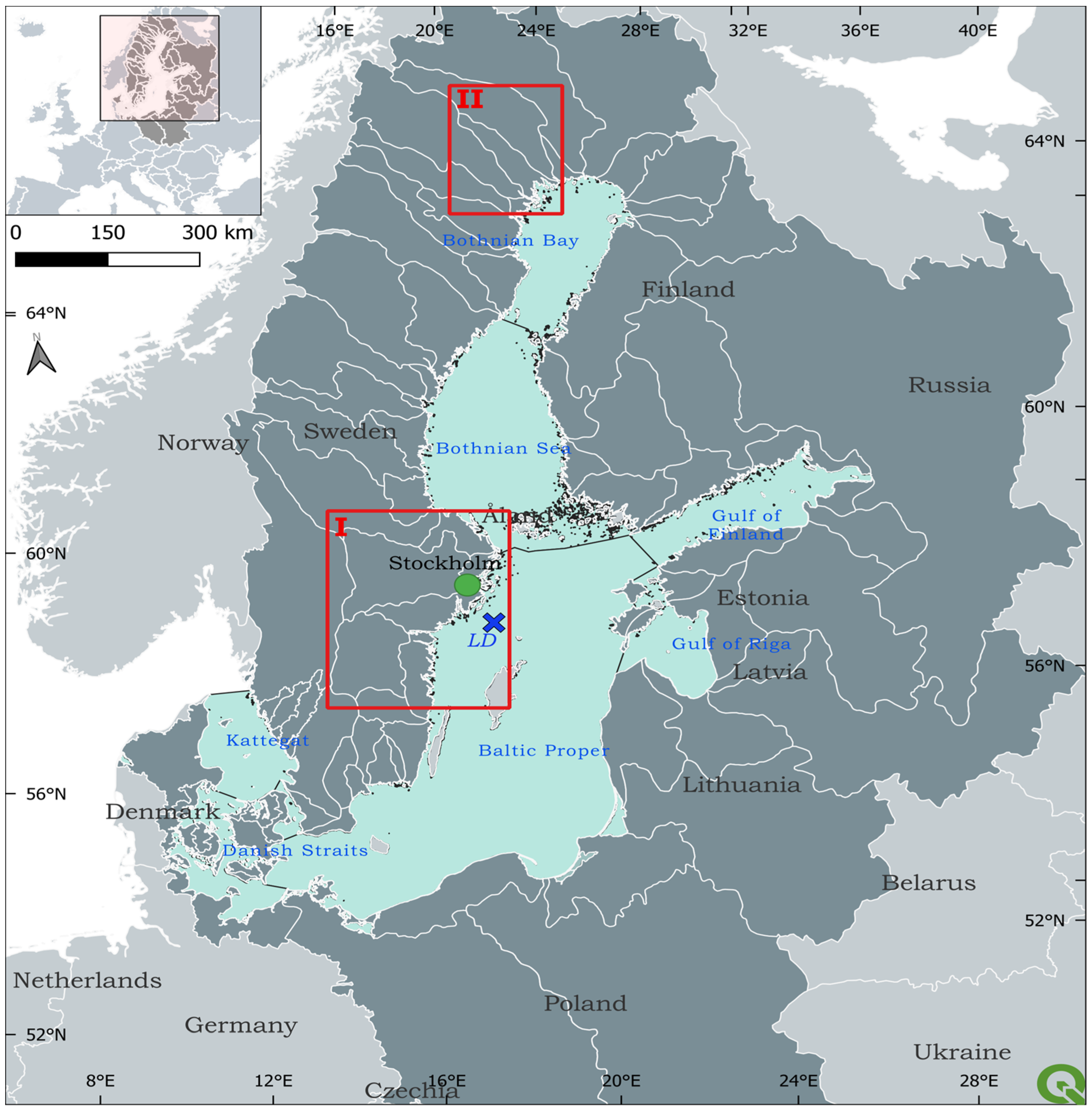
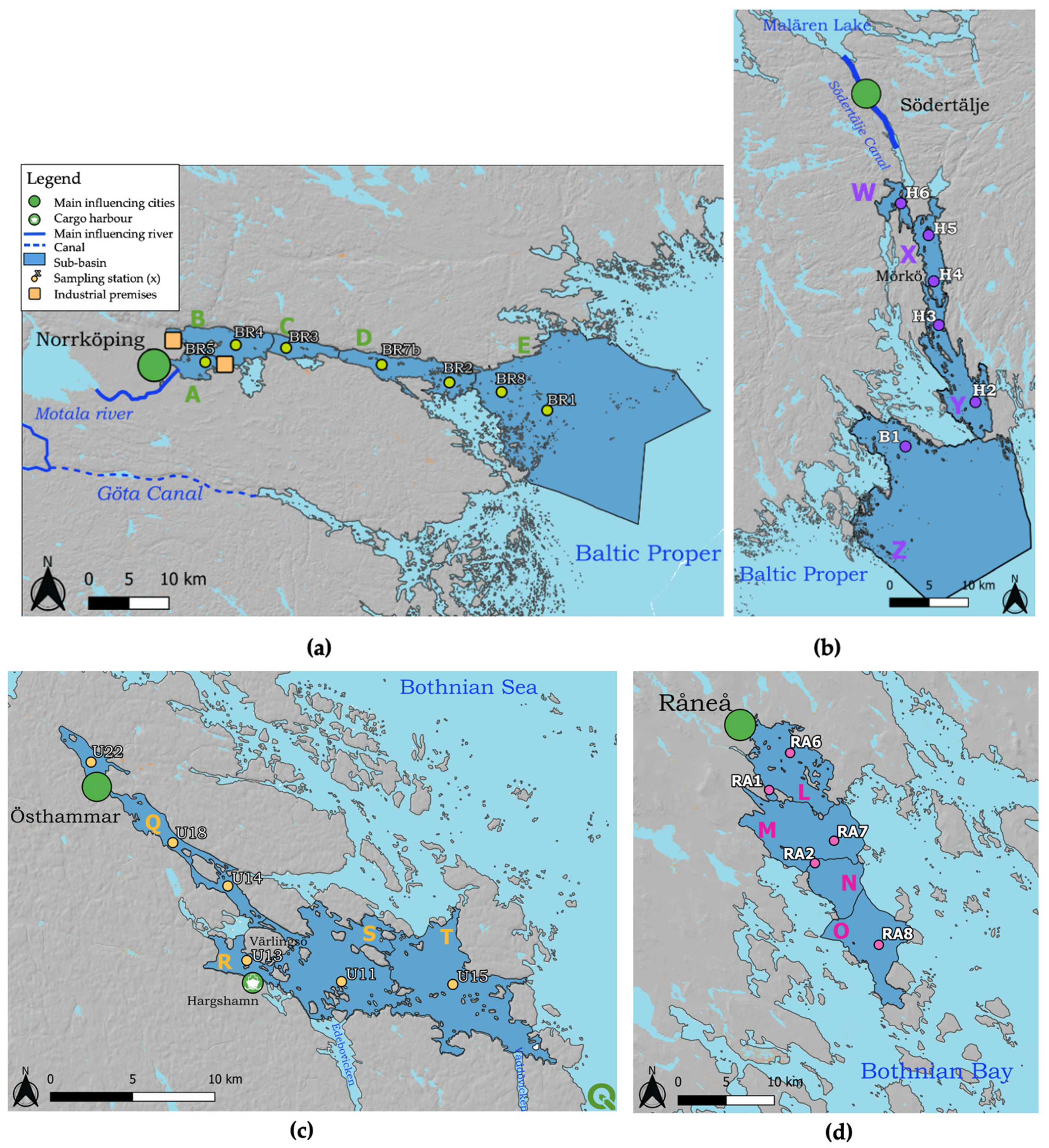
2.1. Site Descriptions

For the analysis, we selected four Swedish bays where measurement transects of optical in-water variables (e.g., Chl-a, CDOM, SPM and turbidity) were performed over the last decade by the Marine Remote Sensing Group (MRSG) and the pelagic Monitoring Group (MG) at the Department of Ecology, Environment and Plant Sciences (DEEP), Stockholm University, and also during 2018 through a collaboration between MRSG and the monitoring group from the Umeå Marine Sciences Centre (UMF), Umeå University.
Figure 1 indicates the two zones of this study: Zone I comprising the northern Baltic proper and the Åland Sea, and Zone II in the northwestern Bothnian Bay. Optical measurements were performed along transects through the different bays (see Section 2.2 below). A numerical analysis of the land cover in the catchments surrounding those bays was carried out using the Geographic Information System (GIS) open source software, QGIS. A catchment is here defined as the natural drainage area, i.e., a zone where rain water flows into streams, rivers, lakes and ground waters, and eventually ends up in certain water bodies (basins) or bays. Section 2.1.1 aims at describing the selected bays and the main surrounding elements (both natural and artificial) that affect these coastal water bodies while Section 2.1.2 explains how the catchments were defined using hydrological data.

2.1.1. Description of Each Site (Bay)

Bråviken bay (Figure 2a) is a large east-west facing bay. Its topography is particularly shallow with a depth gradient from its southern bank (mean depth: 10 m) to its northern bank (mean depth: 40 m). The Swedish Water Archive divides the bay into 5 sub-basins: Pampusfjärden (A), Inner Bråviken (B), Mid-Bråviken (C), Outer Bråviken (D), Bråviken’s coastal waters (E). Several sampling stations (BR1-BR9) of the MRSG (SU) are located along a salinity gradient from the inner bay towards (A) the open sea (E). Many industrial sites are established in the bay and several pulp industry premises are located on the shores of Pampusfjärden and the bay also hosts Europe’s largest grain facility port for export which leads to a lot of ship and boat traffic inside the bay.
Himmerfjärden bay (Figure 2b), is a narrow, elongated bay facing from north to south and it is deeper than Bråviken (40 m mean depth). In the inner bay, there is a sewage treatment plant, which is the third largest in Stockholm County. Himmerfjärden bay consists of several basins that are separated by sills, and is also fragmented by many islands of various size which makes the water circulations more complex than in Bråviken. The water basins in HFj are called Näslandfjärden (W), Himmerfjärden (X), Svärdsfjärden (Y) and Krabbfjärden (Z). Himmerfjärden bay surrounds a central island called Mörkö which hosts recreational sites and natural reserves as well as summer houses. There is a salinity gradient from the inner bay (W) out into the open sea (X), as well as a gradient of optical properties [7]. The optical transects considered in this study starts at station H6 Näslandfjärden (W) going out to H2 in Svärdsfjärden (Y). Station B1 is located in Krabbfjärden in the SW of the island Askö (which is a nature reserve and home of Askö Laboratory, sustained by Stockholm University). Even though B1 is shielded by the island and not part of the chosen optical transect, it has shown to have similar optical characteristics as station H2 just inside Himmerfjärden bay [7]. This is why the optical variable of station B1 and H2 were combined and averaged in the analysis detailed below.
Östhammar bay (Figure 2c) is very shallow and lies in the Åland Sea which is adjacent to the most southern part of the Bothnian Sea. It can be regarded as a bay even though its shape is more complex than those of the other bays of Zone I. Its main branch stretches from SW to NE. Its sub-basins are: Östhammarfjärden (Q), Hargsviken (R), Galtfjärden (S) and Singöfjärden (T). The transect of measurement originates at station U22 towards the outermost station U15, along an increasing salinity gradient. Station U18, U14, U13 and U11 lie in between. At the junction of the sub-basins Q, R and S there is a large island called Värlingsö. The water flows from the inner Östhammar bay (Q) into R where the municipality of Hargshamn is located with its large, industrial port. This part of the bay is deeper than the passage flowing from Q to S-basin, which allows the passage of cargo boats. The water flow is thus more important in the R-S than in Q-S passage. The second inlet branch of the bay is called Edeboviken, where station U12 is usually sampled by the pelagic Monitoring Group (MG) from Stockholm University, but it was rejected from the analysis here because its optical properties have shown to be very different from U13. The presence of Väddöviken bay at the end of the transect might also influence the optical characteristics of the last sampling station U15. The remainder of the bay, i.e., denoted basins S and T (Figure 2c), are fragmented by many islands which makes the circulation of water rather complex.
Råneå bay (Figure 2d) is located in the western Gulf of Bothnia (Zone II, Figure 1), where the waters in the surface layers are frozen during winter, and usually have a very high content of CDOM from riverine sources [24]. The coastal waters are characterized by a very strong coastal influence both after the ice thawing in spring and all during summer. The sampling station RA1, RA2, RA6, RA7 and RA8 are located in 4 sub-basins, stretching from the inner bay towards the outer bay: Rånefjärden (L), Gussöfjärden (M), Tistersöfjärden (N) and Fjusköfjärden (O).
Figure 2. The four Swedish bays, their sub-basins and sampling stations (different coloured circles in different bays) (a) Bråviken, (b) Himmerfjärden, (c), Östhammar (d) Råneå. Note (ac) are situated in Zone I (see also Figure 1 and Figure 3a) and (d) is situated in Zone II (Figure 1 and Figure 3b). Maps generated in QGIS using predefined shapefiles (European coastline shapefile [22]), SMHI’s sub-basin division (havs-områden_SVAR_2016 [23]). Recurrence layer—Global Surface Water, Surface elevation—Copernicus EU-DEM- v1.1; Sentinel Hub [25]).
Remotesensing 16 00176 g002

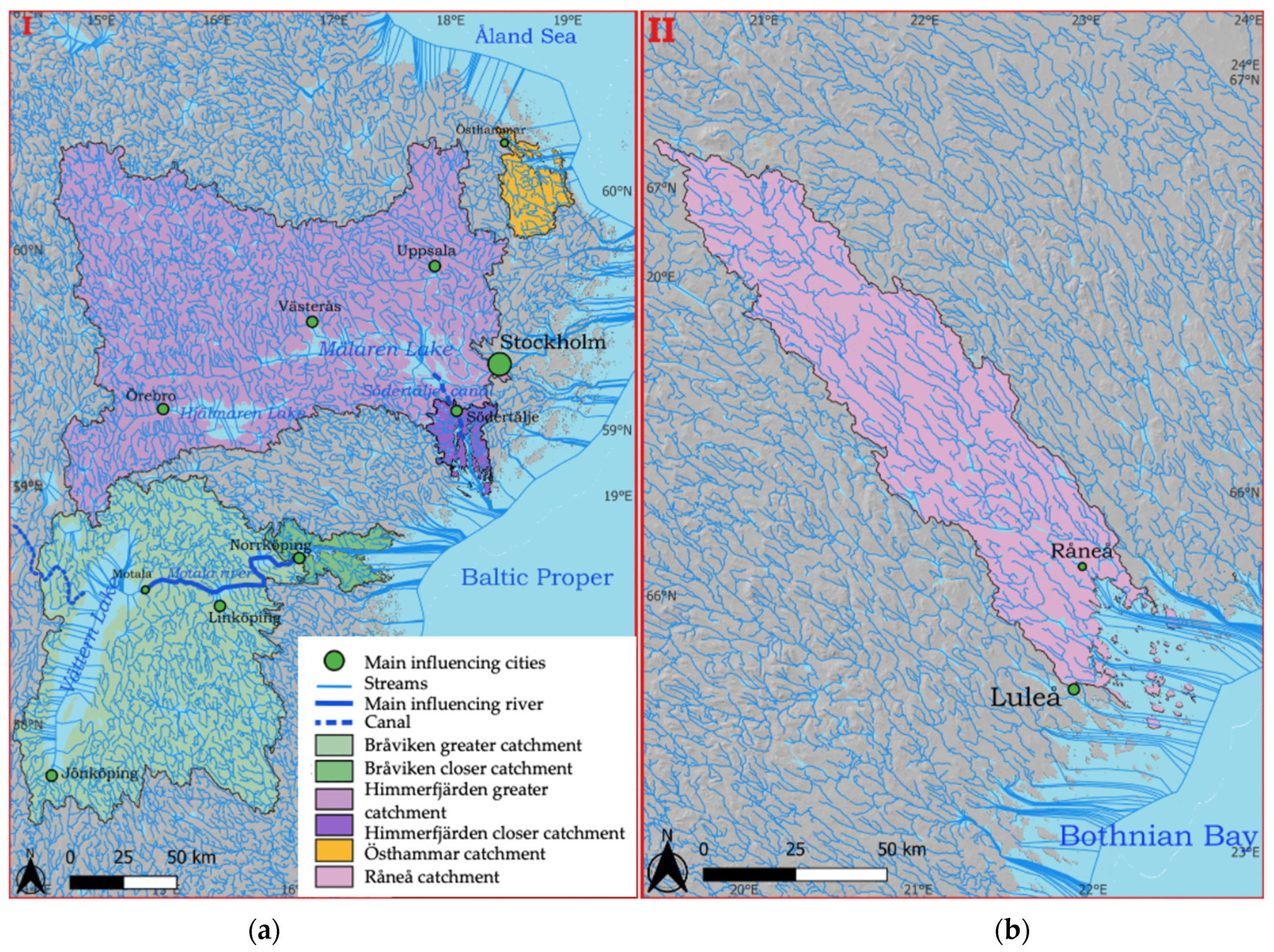
2.1.2. Selection of Catchments

The catchments surrounding the bays were selected based on the Vattenweb (in English: water web) of the Swedish Meteorological and Hydrological Institute (SMHI, Norrköping, Sweden), that can be used to assess the Current Hydrological Status in a certain catchment area [26], as mentioned above, a catchment is defined as an area from which rain and river water flows into other downstream waterbodies. We initially selected both the greater catchment zone for each bay (shapefile haro_y_2016_3) as well as the sub-catchments directly surrounding the bays (shapefile aro_y_2016_3). Eventually, these areas were merged as to constitute the greater catchment zone of interest for each of the 4 bays, respectively (see Figure 3a,b). The average discharge value for each month over the period 1991–2021 and the size of each catchment was derived for each discharge basin, and summarized in an Excel spreadsheet for further analysis.

2.2. Optical Transects

The MRSG performed two satellite validation campaigns in Bråviken bay on board R/V Electra during 1–2 July 2021 and 28–29 April 2022. Optical measurements were taken along transects with a salinity gradient (Figure 2a) from the inner bay (A) out to the open Baltic Sea (E). The data from the field campaigns in 2021 and 2022 were merged with other transects from past expeditions performed over the last decade in the four bays (Figure 2, Table 1). The MRSG has trained the pelagic monitoring groups at Stockholm and Umeå Universities on how to perform optical measurements (e.g., CDOM, SPM and turbidity) and the groups share their optical protocols and also intercompare their methods [27]). Table 1 provides a summary of the measurements performed, including dates, operating group and number of samples gathered. Altogether, n = 116 stations were sampled for this study, including measurements of Chl-a, SPM, SPIM, SPOM concentrations, turbidity, Secchi Depth, CDOM absorption, aCDOM, and the CDOM slope factor, SCDOM. The largest collection of data comes from the Himmerfjärden area.

2.2.1. Water Sampling and Measurement Protocols

Note that the procedures below follow the Optical Measurement Protocols of the Marine Remote Sensing Group. During the field work, the samples were gathered 20–30 cm below the water surface with a sturdy sampling bucket with a pip. The bucket was rinsed twice with sea water before sampling as to avoid contamination. The sampling bottles were also rinsed twice with sea water and then filled with sea water from the bucket. The same standard protocol was applied for all other field campaigns by the MRSG but other laboratories sometimes have slightly different protocols. Nonetheless, intercomparison workshops are held regularly to make sure that the measurements between groups are comparable.

SPM, SPIM and SPOM Measurements

Depending on the Secchi depth reading, 1–2 L of sea water were sampled for SPM measurements. The measurements were performed using the gravimetric method [7,28]. This method consists of filtering a certain quantity of natural water through microfibers glass filters (GF/F filters) of 47 mm diameter and with a nominal pore size of 0.7 µm. Before filtration, the filters were pre-rinsed with ultra-pure water (UPW), combusted and pre-weighed (tare weight) with a high-precision scale (Satorius MP3 microbalance—±1 µg). Each sampling bottle was gently mixed before filtration to ensure even distribution of suspended material. All filters were rinsed at the end of the filtering process with 100 mL UPW for removal of salt residuals. After filtration, each filter was placed in a numbered (by etching), clean square aluminum foil (10 × 10 cm). Then, the filters were dried overnight at 60 °C. The filters were subsequently stored in a desiccator in order to keep them dry until weighing. The dry weight of SPM was derived by subtracting the tare weight from the dry weight. In order to derive SPIM, the filters were combusted for 5 h at 480 °C, and were weighed again. The organic fraction was then derived from the weight difference between the total SPM (dry weight) and the SPIM (combusted weight), assuming all organic matter has been combusted. The handling of the filters sometimes leads to the loss of filter bits. Therefore, triplicate filters were taken for every station as quality control of the measurements. Outliers were removed if the standard deviation was more than 20%. For every field campaign between 5 and 10 blank filters were processed in the same way except that ultra-pure water (UPW) was used (0.5 L) instead of sea water, and their average weight was then used to correct for handling errors. In the Bothnian bay, the rinsing with UPW was sometimes omitted by mistake by the local monitoring group, and during the data quality control (i.e., comparison against the measured turbidity values), the samples were found to be invalid and therefore had to be omitted from the final analysis.

Turbidity Measurements

Turbidity was measured during field campaigns with a portable turbidity meter (Hach Lange 2100Qis, HACH LANGE GmbH, Düsseldorf, Germany). The calibration of the device is performed using standard formazin solutions of known turbidity (10, 20, 100, 800 FNU). Formazin Nephelometric Unit (FNU) is a unit equivalent to NTU but is measured in the near infrared (NIR) rather than using white light. The standard calibration solutions are provided by the manufacturer. Before performing a measurement, one gently mixes a sample [16]. It is important to wait for 10 s before starting the measurement in order to remove air bubbles that could cause extra scattering, and thus wrongly increase the turbidity value. Each turbidity sample was measured 5 times and the values were averaged and corrected for the average turbidity value of ultrapure water (UPW) which was also measured 5 times.

CDOM Measurements

The CDOM samples were collected in 250 mL amber glass bottles and the samples were filtered through 0.22 µm membrane filters using glass filtration unit fitted with a metal mesh to avoid clogging of the filtering unit. The filtrate was then transferred into 100 mL amber glass bottles and stored in a refrigerator at 4 °C for up to 3 months. The absorption spectra of CDOM was measured by scanning the sample in a Shimadzu UVPV-2401 dual beam spectrophotometer (Shimadzu Corporation, Kyoto, Japan). Before scanning, the samples were removed from the refrigerator and allowed to reach room temperature (overnight). The absorption spectrum was measured in the range from 350 to 800 nm in cylindrical quartz cuvettes (10 cm). First, a baseline was performed, using both cuvettes filled with UPW. The cuvette in the back was then used as a reference (UPW) while the front cuvette was filled with the respective water sample and scanned. The absorbance was measured from 190 to 850 nm (in 1 nm steps). The absorbance at 700 nm was then used to correct for measuring errors, and the spectral absorption for CDOM was derived from the following relation, according to Kirk [1]:
a C D O M ( λ ) = ln ( 10 ) OD ( λ ) L 1 ,   [ m 1 ]
where OD ( λ ) being optical density (absorbance), L being the optical path length of the cuvette in meter, here 0.1 m. Note that the OD is measured in logarithmic values (Ln10). The CDOM absorption at 440, aCDOM, is then derived per meter after log transformation. Then, the whole absorption spectrum is log transformed and the slope of the derived line (in the range of 350–500 nm) corresponds to the slope factor of CDOM, SCDOM.

Chlorophyll-a Measurements

0.2–0.5 L of sea water were filtered onto 25 mm diameter GF/F filters. Filtering was performed on board ship and the filters were flash-frozen in liquid nitrogen and stored for up to 2 months. Each sample was filtered and measured in triplicates. Before the spectral analysis, the samples were placed in 5 mL of 90% acetone solution and sonicated for 30 s for destruction of the cell walls and extraction in acetone. The samples were then centrifuged for 10 min at 3000 rpm so that all particles could settle in the bottom of the polypropylene test tube and thus avoid the effect of scattering on the absorption spectrum. After 30 min of extraction, the samples were transferred into 1 cm quartz cuvettes and scanned against 90% acetone (350–850 nm) in a UVPC-2401 dual beam spectrophotometer (Shimadzu Corporation, Kyoto, Japan). The spectra were then processed in Excel (2019) with the algorithms and coefficients provided by Strickland and Parsons (trichromatic method) [29] in order to derive the Chl-a concentration in µgL−1. This method has shown to be within 10% error during an inter-calibration performed by the ESA MERIS Validation Team [30] and within 2–10% when compared to the Swedish monitoring groups [27]. The method has also been intercompared regularly with HPLC measurements [27,30].

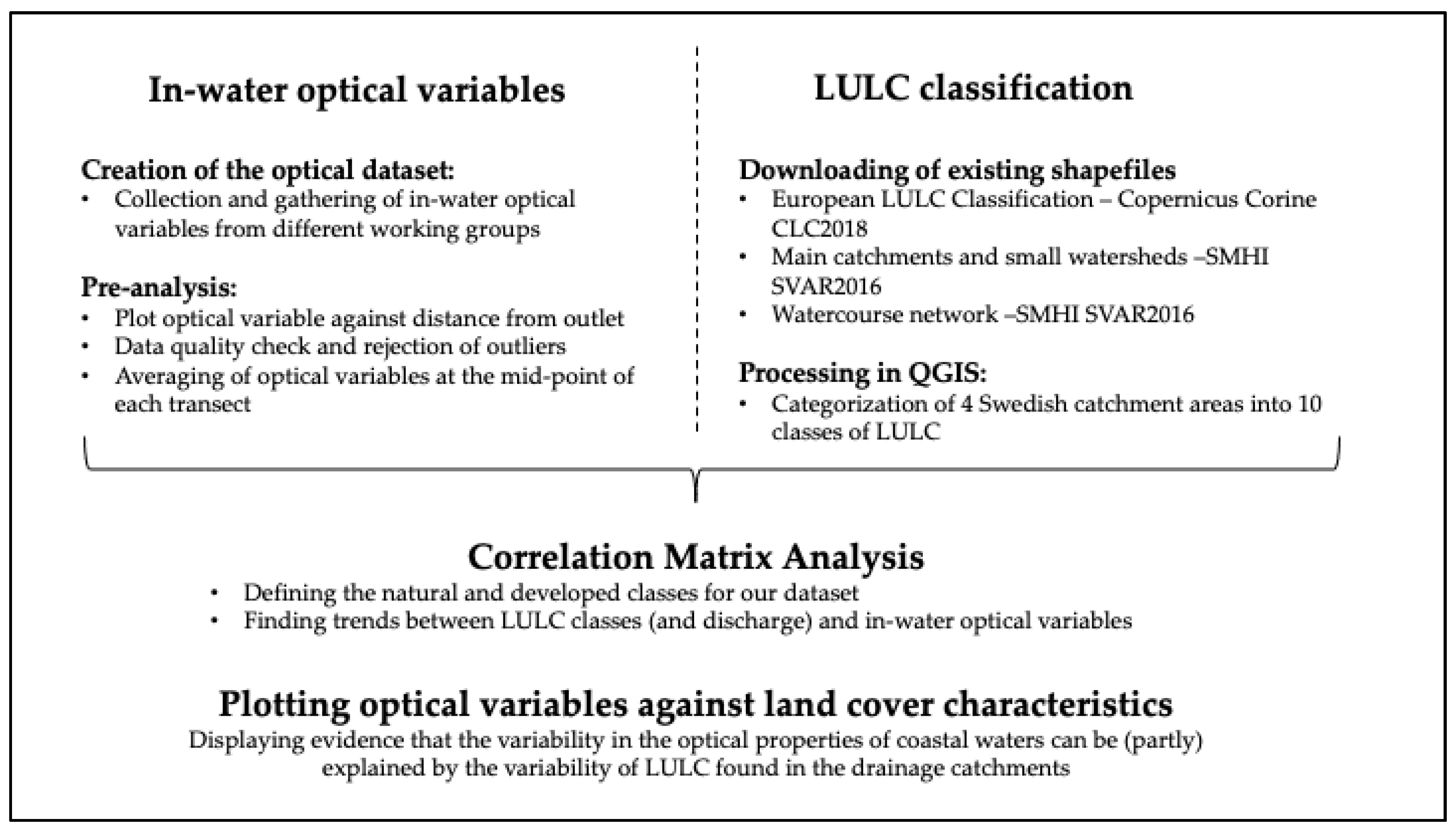
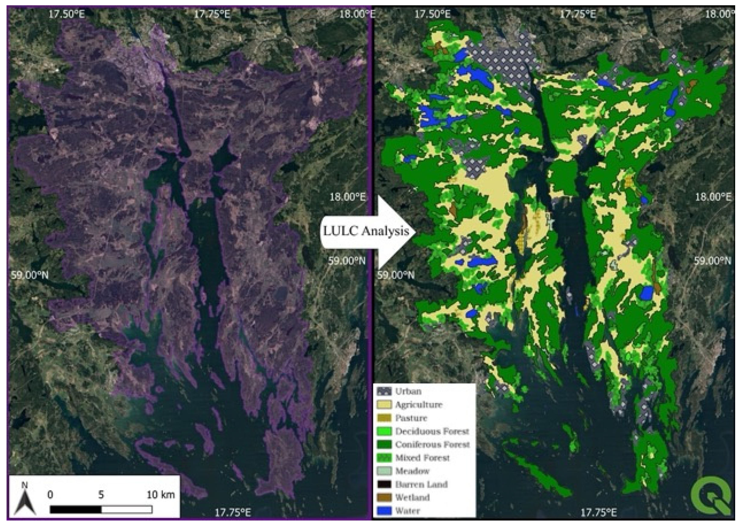
2.3. Land Use and Land Cover Analysis

The land use and land cover (LULC) of each bay was analyzed in QGIS (version 3.26.2 ‘Buenos Aires’), an open-source Geographic Information System (GIS). Data from two sources were used to define the extent of the catchment of each bay. Firstly, shapefiles from the Swedish Hydrological Meteorological Institute (SMHI), provided the polygons shapefiles of the Swedish catchments (Haro) and sub watersheds (aro) around the different bays of the study using SVAR version 2016_3 [23]. Maps of the different catchment areas are shown in the results section in Figure 3. The final catchment area selection was not trivial and was performed with regard to modelled hydrological data from the SMHI’s Water Web [26].
Secondly, we used the CORINE Land Cover 2018 (CLC2018) dataset derived from Landsat-8 satellites images [25] for the LULC classification. These products are based on data from 2017 to 2018 and have a 100 m resolution with a thematic accuracy of ≥85%. They are generated regularly in 6-yearly cycles. The CLC2018 dataset was published in 2020 and provided initially 44 land cover categories (see Supplementary Table S1) which were further aggregated into 10 classes for this study. The following operations were performed to process the data in QGIS:
  • Reprojection of CORINE into the same geographical projection as for the Catchment shapefile EPSG3006 SWEREF99 TM used by the Swedish Meteorological and Hydrological Institute, SMHI, Norrköping, Sweden [23].
  • Fixing geometries of CORINE data via the vector operation “fix geometries”.
  • Reducing the number of Level 1 attributes from 44 to 10 categories (so called Code 18).
  • Aggregating the original 44 to 10 polygons of the same Level 1 class.
  • Intersection of the dissolved LULC polygons with the catchment boundaries in order to exclude information outside the areas of interests.
  • Eventually, computation of percentage area per category of Level 1.
All 11 urban classes from the original 44 classes were thus aggregated under the class Urban. All arable land, permanent crops and heterogeneous agricultural areas (consisting of 10 classes) were aggregate into Agriculture. The class Pastures was left as designated by CORINE. It may differ from the Agriculture class due to the manure from cattle, and also from the class Meadow which refers to land that is covered by different natural grass types and bushes. All open spaces with little or no vegetation were assembled into one class: Barren Land. The four shrub/herbaceous vegetation classes were aggregated into one Meadow class. All 5 wetland categories were aggregated into a Wetland class. Similarly, the 5 water subcategories into one Water class. Deciduous Forest, Coniferous Forest and Mixed Forest were left unchanged.

2.4. Combining Optical and LULC Data

All data were collected and processed in Excel for further analysis. A first analysis was performed in order to operate a data quality check. From the geographical coordinates of a given station the horizontal distance from an outlet was derived (in km) with the aim to make the transects within the 4 bays comparable. The outlet was chosen to be either a defined river mouth (cf. Östhammar and Råneå), or the innermost station usually sampled by the respective monitoring or research group (cf. station H5 and BR5 in Himmerfjärden and Bråviken). A new data sheet was then compiled for each optical parameter, and various plots were made to visualize the data, either season-wise or regardless of the time of the year. It allowed to identify outliers and observe variability between the bays as well as seasonal variability, and to choose which variable to focus on.
Finally, the stations were aggregated based on their horizontal distance from the outlet. The mean horizontal distance from the outlet ranged from approximately 15 ± 5 km in the different areas. Any innermost or outermost station making the mean distance deviating from this range were rejected from the study in order to make the datasets comparable. The optical properties in each transect were then averaged by taking the mean values from geographic middle stations, the rationale being that this allows for a comparison of the different bays of different sizes, and across different times of year. Note that the derived optical products are thus averaged over space and time for every transect. Eventually, the optical variables were plotted each against a LULC information, such as a percentage of a given land cover, or a ratio of several land covers which helped to identify the main trends.
Additionally, a correlation matrix was prepared to identify possible links between LULC class and optical variables. The correlations in the matrix were then tested using a significance test based on the p-value test ( α = 0.05 ) . The workflow of the analysis is summarized in Figure 4.
Le et al. [19] had observed in their study that groups of LULC categories could be assembled in order to relate them to optical properties on a macroscopic scale. They derived a Natural category (Coniferous Forest + Wetland) as well as a Developed category (Urban + Agriculture). Eventually, they inferred that the Ratio Developed/Natural category showed interesting results when comparing to the optical properties of various estuaries in their study. As a first step, such group categories and ratios were also derived and tested for this study but were also adapted with regard to our correlation matrix and typical trends observed in Swedish bays (see results of the correlation analyses and trend analysis below). The natural class used here, denoted Natural*, was thus merged to include Coniferous Forest + Wetland + Meadows while the developed class, denoted Developed*, included Urban + Agriculture + Pastures (although the latter was so small in % area that it did not show any effect on the results; see below). Finally, the ratio of Developed* over Natural* was denoted Ratio*. Correlations were applied between optical properties and the final LULC categories as well as the grouped categories Natural*, Developed* and Ratio* as defined above, and also between optical properties and the discharge values derived for the different bays from the Current Hydrological Status on the SMHI Water Web [26].

3. Results

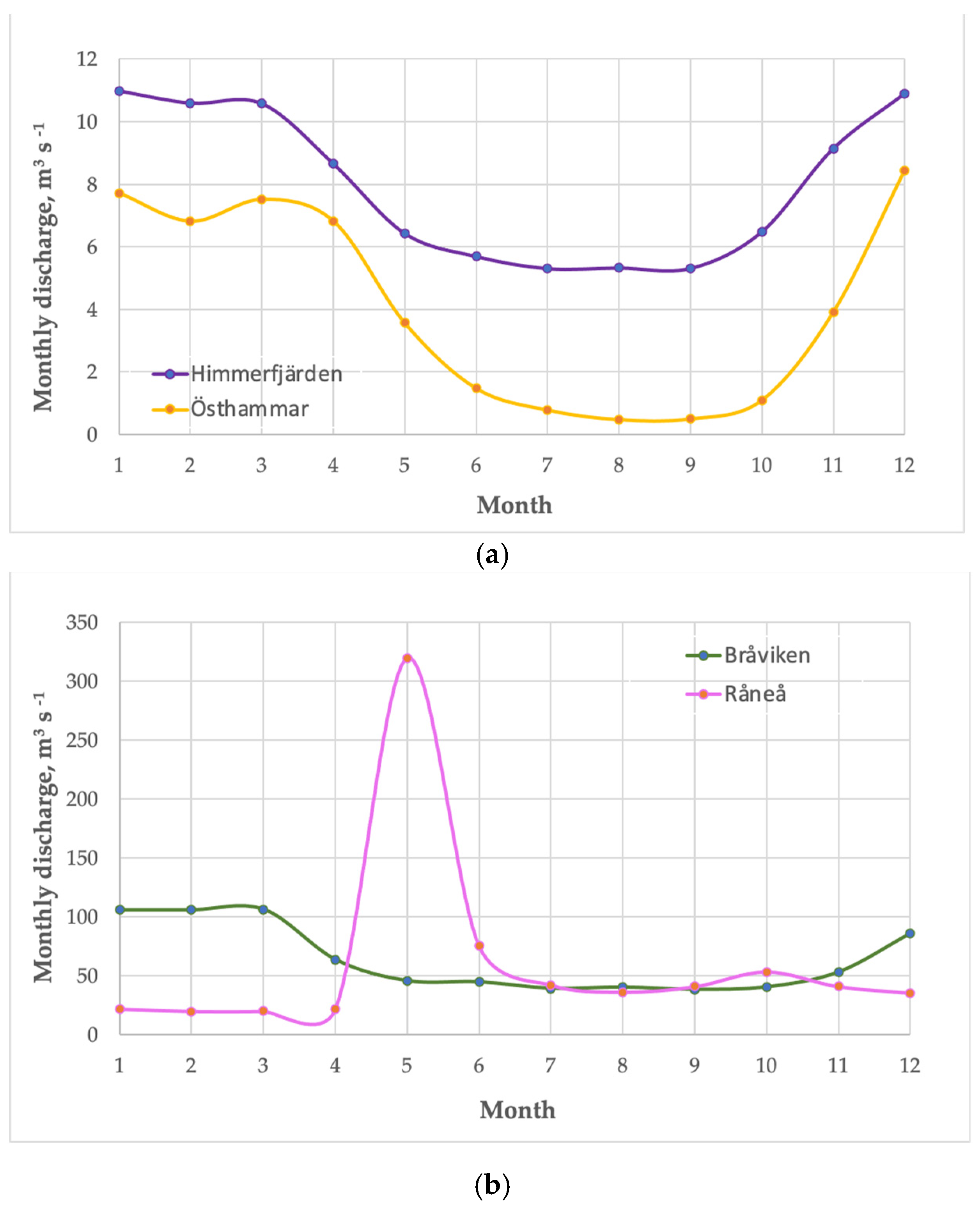
3.1. Derived Catchment Areas and Description of Their Hydrology

The derived catchment areas varied from only 993 km2 for Östhammar bay to 23,368 km2 for Himmerfjärden bay (Figure 3). Due to the large differences in surface area and hydrology, the monthly and yearly discharge varied considerably in and between bays (see Figure 5 and Table 2). Himmerfjärden has the lowest yearly discharge with approximately 49 m3s−1, followed by Östhammar bay with approximately 95 m3s−1. Bråviken bay and Råneå bay show a substantially higher yearly discharge of approximately 766 m3s−1 and 725 m3s−1, respectively. It must be noted that in Råneå the monthly discharge is much lower from January to March (approximately 20 m3s−1), while there is a very high peak stretching over April to June due to the ice melt in spring.
The Bråviken catchment (Figure 3a) is composed of two parts—its greater catchment (light green) and its surrounding catchment (dark green). The Motala river is connected to Lake Vättern and leads into Pampusfjärden (area A, Figure 2a) passing through Motala, Linköping, and eventually Norrköping. Lake Vättern, with a total surface area of 1912 km2 is the second largest lake of Sweden and the sixth largest lake in Europe.
It thus generates a considerable monthly freshwater flow of approximately 50 m3s−1 at its source in Motala, gathering even more discharge water on its way to Norrköping where the water flow reaches approximately 100 m3s−1 in winter and spring, and approximately 50 m3s−1 in summer and autumn (Figure 5). Vättern also exhibits downstream connections with the Göta Canal, while one section flows down into Lake Vänern and another into the Baltic Sea, but the water flows are negligible when compared to Motala river (less than 1 m3s−1).
The water in Himmerfjärden bay originates by approximately 50% from the streams of its surrounding catchment (dark purple) and ca. 50% from its greater catchment (light purple), collecting all the discharge water into Lake Mälaren (Figure 3a). Unlike the greater catchment of Bråviken, it is not connected by a natural river but with the Södertälje Canal, named after the town it passes through. This canal is regulated by locks and has a very low and almost constant flow of freshwater of approximately 5 m3s−1. During events of floods and heavy rainfall, the locks can be opened up to alleviate the flooding risk in Stockholm City and the discharge jumps then suddenly up to 100 m3s−1, but these kinds of events are quite rare and did not occur during any field campaign considered in this study.
The Östhammar bay receives its waters from various streams and small rivers (Figure 3a). The catchment includes many small lakes and minor bogs which explains why the water outflow is only approximately 4 m3s−1 on a yearly average.
The landscape in the Råneå catchment is highly influenced by a myriad of various streams, converging into the Råneå river (Figure 3a). The shape of the monthly discharge curve along the year is remarkably different from the catchments of Zone I (Figure 5b). A major peak in mid-May can be observed induced by the thawing of sea ice and snow. It gives rise to a very large monthly discharge of approximately 320 m3s−1. The inflow of freshwater decreases to approximately 50 m3s−1 during July, and then progressively further down to ca. 20 m3s−1 during the winter months.

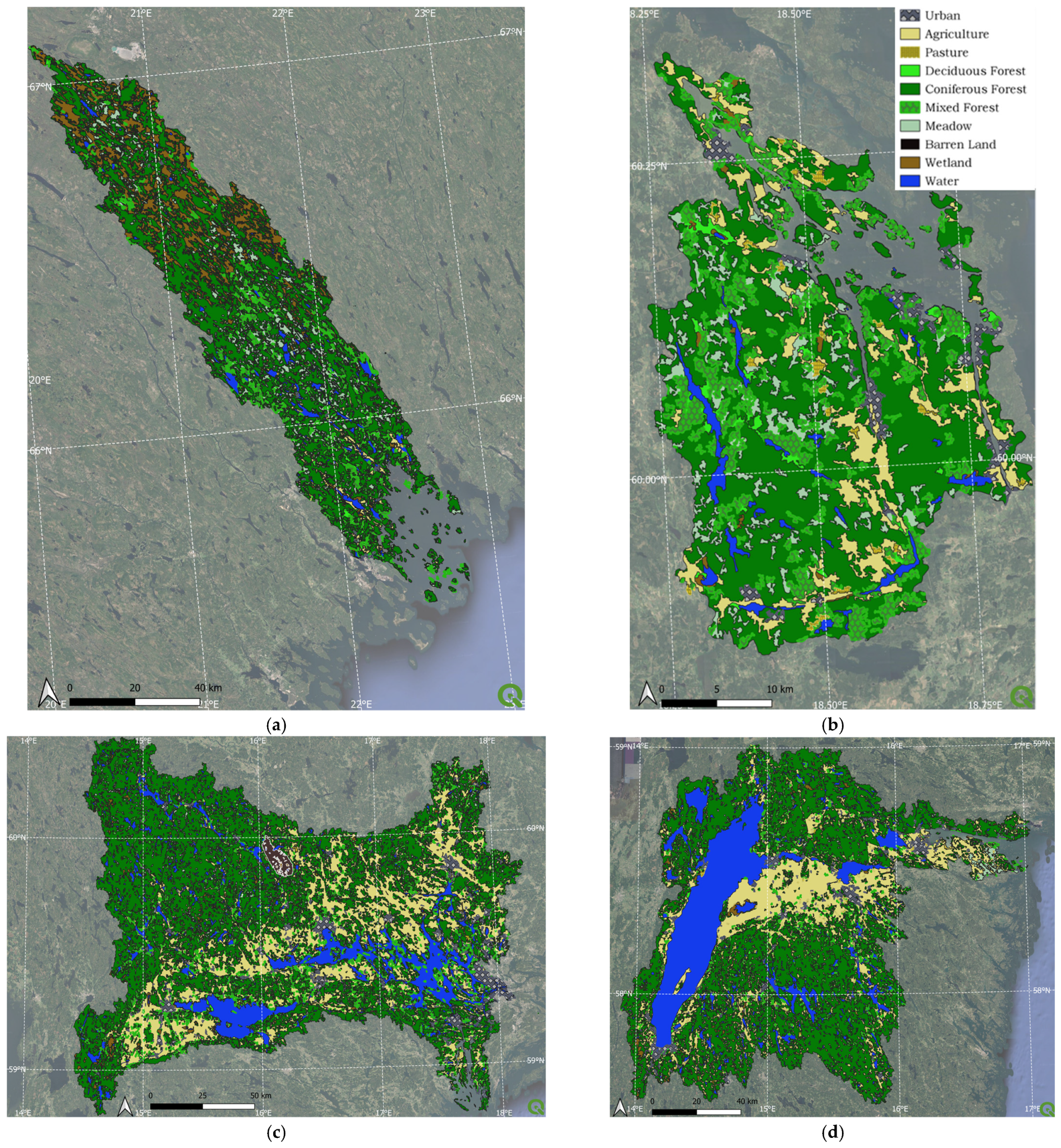
3.2. Results of the LULC Analysis

Figure 6 shows the map of Himmerfjärden bay and its closer catchment area before and after the LULC analysis was applied.
The results of the LULC classification for all four bays are listed (as % coverage) in Table 3 and shown in Figure 7 (see also enlarged images in Supplementary Figure S2c,d). The catchment areas of Himmerfjärden bay (Figure 7c) and Bråviken bay (Figure 7d) exhibit quite similar land cover profiles, except that Himmerfjärden is more artificially developed due to its slightly more important Agriculture and Urban classes The Råneå estuary stands out with a much more Natural profile (Figure 7a). In this part of Swedish Lapland, the flora is not only dominated by Coniferous Forest but also by vast Meadows (13.2%) and Wetlands (19.1%). Östhammar, located slightly to the North of Stockholm archipelago, displays an intermediate profile between that of Råneå, Himmerfjärden bay and Bråviken bay. On the one hand, Agriculture (11.3%) is the third most important class, but to a lesser extent than for Bråviken bay (20.0%) or Himmerfjärden bay (23.2%). On the other hand, its Forest coverage is more similar to that of Råneå bay.
Table 3 also shows that the leading LULC class in each catchment area is the class Coniferous Forest. This is very typical for Swedish forests which are dominated by spruce and pine which together make up approximately 80% of tree coverage [31]. Overall, Agriculture was the second most important land cover type except in the more pristine area Råneå in the northwestern Bothnian Bay. Furthermore, Mixed Forest made up 4.3% to 14.3% across all catchments, while the Water class was also important in the catchments of Bråviken (18.4%) and Himmerfjärden (10.6%) due to the influence of Lake Vättern (Bråviken) and the combined influence from Mälaren and Hjälmaren (Himmerfjärden).

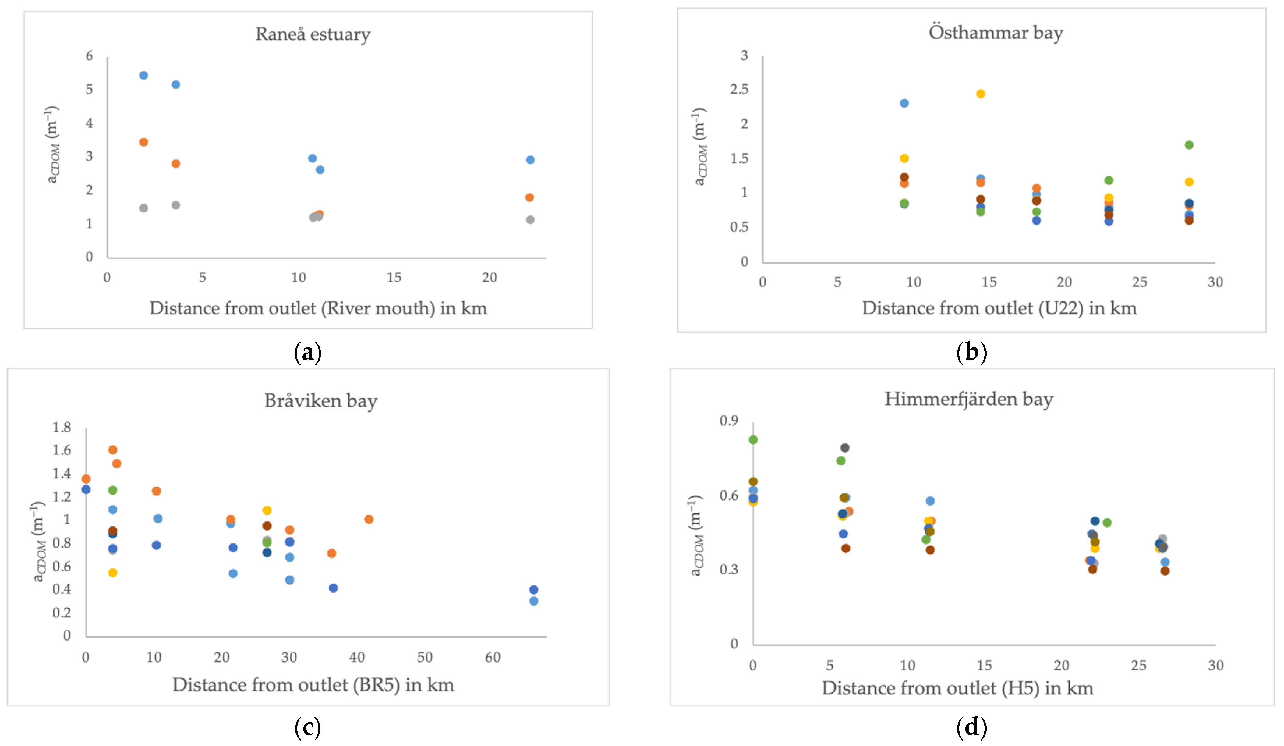
3.3. Ranges of Optical Properties in Each Bay

Table 4 gives an overview of the minimum and maximum values of the optical properties in each bay, as well as the median and the number of observations (n).

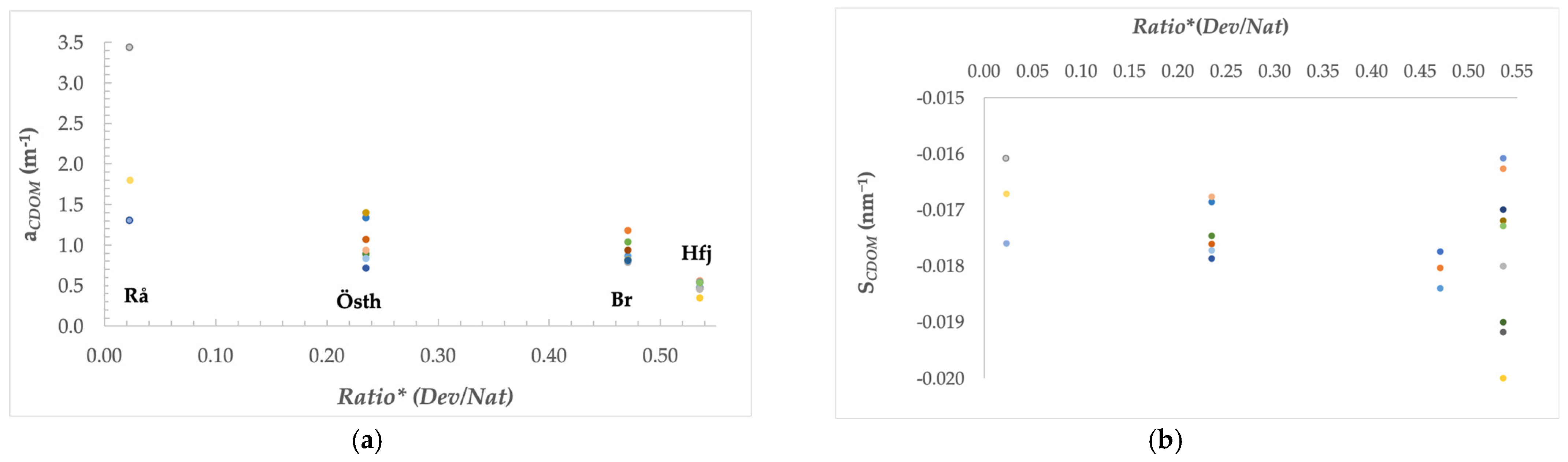
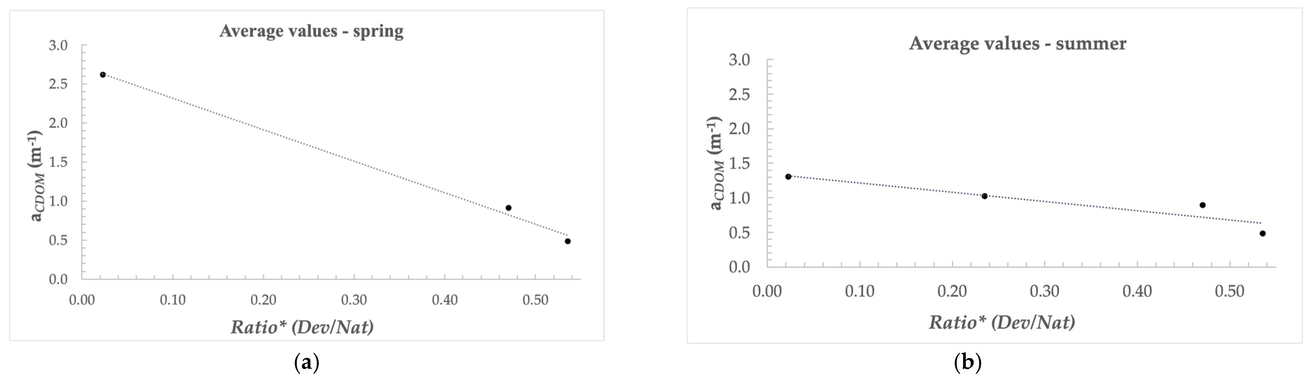
3.4. Investigating the Nature of CDOM Due to LULC

Figure 8 displays CDOM absorption at 440 nm, aCDOM (440) against the distance from the outlet for each respective bay (data from all seasons and years included). The maximum CDOM values were found in Råneå (up to approximately 6 m−1) during the transect in May 2018, which corresponds to the snow and ice thawing period. At that time of the year the average water catchment discharge, Q, is approximately 300 m3s−1 (Figure 5b). The results from the correlation analysis of LULC categories vs. aCDOM and SCDOM, respectively are shown in Table 5.
In Figure 9a one can see how aCDOM is related to the ratio of Developed to Natural classes in the wider catchment areas. The lower the proportion of developed areas, i.e., Ratio* (Dev/Nat), the higher the CDOM absorption. The results show that Råneå bay has the most natural catchment with a Ratio* (Dev/Nat) of approximately 0.023, followed by Öshammar bay (0.235), Bråviken (0.47) and Himmerfjärden bays (0.535). Figure 9b shows that the average CDOM slope factor per transects is also dependent on the ratio of developed to natural areas, and there is a negative trend over the four bays, although Himmerfjärden shows a large spread of data. Seasonal variability can be here rejected as explanation as both the highest (August 2010) and lowest value (August 2017) were both obtained during measurements in summer. The large variability in Himmerfjärden bay is likely to be due to the influence of Himmerfjärden Sewage Treatment Plant situated in the inner bay, where nitrate is treated by bacterial breakdown [31]. In addition to breaking down nitrates, the bacteria may also use CDOM as a substrate, and break down the larger humic acids to fulvic acids. On the other hand during periods of flooding, untreated stormwater may enter the bay, and thus giving rise to larger humic acids. The decreasing trend from Råneå to Bråviken in Figure 9b indicates that more natural LULC types will generate more humic acids, whereas the more developed bays tend to have a lower spectral slope factor, and thus contain a higher proportion of fulvic acids.
Figure 10 shows that there is a clear difference in the spatial trend of aCDOM across the bays between spring and summer. aCDOM is especially high in the Bothnian Sea during spring presumably due to the high coastal runoff after the spring melt, bringing in high concentrations of larger humic acids [5].

3.5. Investigating the Nature of Particulate Material with LULC

Overall, the suspended particulate matter (SPM) and turbidity correlation analyses did not show such clear trends as CDOM absorption and slope across the different areas of interest, apart from suspended particulate organic matter, SPOM (Table 6), which showed a positive significant relationship with the LULC classes Coniferous Forest, Mixed Forest and Meadow, and thus with the Natural* classes, while it showed a negative relationship with Agriculture, and the ratio of developed to natural classes (Ratio*).

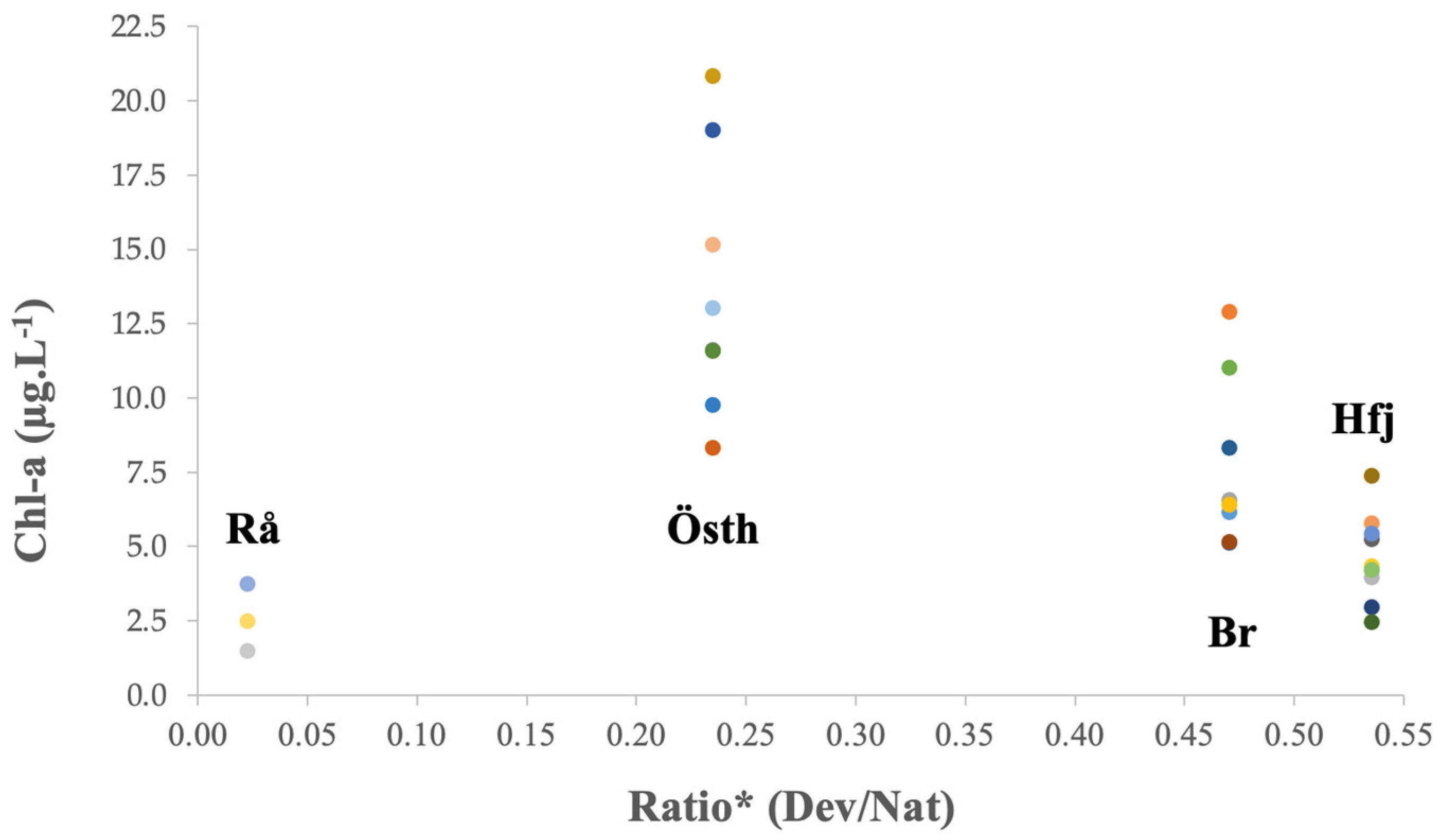
3.6. Investigating the Dependency of the Chl-a Concentration on LULC

The correlation matrix (Table 7) shows significant negative correlations for Chl-a with the classes Agriculture, Wetland, and developed classes (Dev*), as well as the ratio of developed to natural classes (Dev/Nat).
Figure 11 displays the average Chl-a values for a given field campaign plotted against the ratio of developed to natural classes (Dev/Nat) LULC. The Råneå bay clearly stands out with its relatively low chlorophyll-a concentrations, both in spring and summer. This is likely to be related to the high CDOM absorption with very large values found in coastal areas of the Bothnian bay (Figure 8a). Indeed, the strong light attenuation by CDOM in this area has been shown to limit the growth of phytoplankton and algae, and instead to favor bacterial production [23]. Since the Råneå measurements clearly stand out when compared to the other bays, it has been rejected from the correlation matrix for the remainder of the analysis. The motivation for this is that the relatively low Chl-a levels here are most likely due to light limitation by CDOM rather than caused by different LULC categories.

4. Discussion

4.1. LULC Classification

The land use and land cover (LULC) analysis is central in this study, focusing initially on analyzing the variation in LULC from one Swedish bay to another. Our LULC classification (Table 3) gave a similar result as the one performed by Franzén et al. [32] who classified the sub-catchment area around Himmerfjärden with 57% forest, 33% land, 4% lake and 5% urban areas. We decided to use the great catchment in our study, assuming that the optical properties in the whole catchment are carried downstream, and therefore influence the optical properties of the bay. Gullstrand et al. [33] classified Bråviken with 49% forest, 18% agriculture and 20% water which, again is quite similar to our classification (Table 3), even though we decided to include the greater catchment rather than just the surrounding catchment of the bay. As the bays also differ in their surrounding and catchment areas, it is likely that the bio-optical properties are influenced by the variation in the land cover and land use in each area. Table 3 shows that the leading LULC category in each catchment area is the category Coniferous Forest, followed by Mixed Forest. The dominance of Coniferous Forest is very typical for Swedish forests [34]. Our LULC analysis also confirms previous work showing that catchments in boreal regions are mostly covered by Coniferous and Mixed Forest [35], carrying high concentrations of terrestrial dissolved organic matter (DOM) downstream during the productive seasons. Additionally, there are usually wetlands and bogs in boreal areas, which have the tendency to hold large quantities of organic matter [36]. CDOM usually increases in spring after the ice melt, followed by a decrease in summer and an increase, again, during autumn [5,37]. Said Al-Kharusi [38] proposed that recent advances in remote sensing technology, GIS and modelling could improve our understanding of CDOM in inland waters on large geographic scales. The same has been demonstrated here for the distribution of CDOM in coastal waters.

4.1.1. Influence of LULC Classification on aCDOM and SCDOM

As shown in the results section, aCDOM and SCDOM are both positively related to Wetland, and the Natural* LULC classes while they are negatively correlated to Agriculture and the Developed classes. Zheng et al. [39] found positive correlations for aCDOM and SCDOM with the natural categories Forest and Grassland in the yellow river basin. An explanation why we did not find a significant positive correlation with Forest might be that our forests are mostly dominated by coniferous trees. Dead plant material is slowly degraded to humic substances by bacterial breakdown [1]. During droughts, it accumulates on land, and during floods and the spring melt it is washed into lakes and coastal waters [38,40,41]. The minimum range of CDOM values (approximately 1 m−1) is found in Himmerfjärden bay (corresponding to the average value in the middle of the transect). Note that Zone I does not exhibit any strong peaks in discharge for the thawing in spring, based on the hydrological data from SMHI [26]; see Figure 5.
The results shown in Figure 10a,b clearly indicate a seasonal variability in the CDOM absorption. The results show a steeper (decreasing) average slope in spring than in summer. According to the correlation matrix (Table 3), Wetland and Meadows showed significant and positively correlated coefficients with the CDOM slope factor. With an increasing proportion of wetlands and meadows, the humic types of CDOM thus seem to increase as indicated by a CDOM slope closer to −0.0011 [4].
We also find that the categories Agriculture, Developed and also Ratio* each show a significant, negative correlation with SCDOM. The influence of developed categories is more difficult to interpret. One explanation could simply be the degradation of CDOM in natural environments, either by UV light (a phenomenon called photobleaching, or fading) and degradation by bacteria [1]. Indeed, CDOM is naturally broken down progressively—chemically or physically—in these ways. For instance, Hulatt et al. [42] found that photo bleaching can cause a significant increase in the spectral slope factor (by 0.004 nm−1), that is to say that CDOM tends to be progressively more broken down into smaller fractions, and thus tends to have a more fulvic profile (i.e., a slope closer to −0.0022). Therefore, Agriculture and other developed categories might influence the CDOM slope factor by enhancing the decomposition of CDOM. Williams et al. [43] found that dissolved organic matter (DOM) in streams influenced by agriculture was more labile and more accessible to microbial degradation than DOM found in wetland streams, supporting lower rates of microbial activity. Such result suggests that the Developed* classes of LULC will be likely to stimulate bacterial breakdown of CDOM, and thus be more likely to generate a higher content of smaller fulvic acids.

4.1.2. Influence of LULC Classification on SPM

As mentioned before, there were no obvious relationships between total SPM and LULC cover. However, for suspended particulate organic matter (SPOM) significant and robust relationships were found for the classes Coniferous and Mixed Forests, as well as Meadows and the categories Natural* and Ratio* (see Table 6) while the Agricultural class showed a negative but significant correlation. One could explain the positive correlations with predominantly natural categories by the fact that they generate a lot of pollen in spring and summer. Pollen constitutes indeed an important fraction of SPM in natural waters [44] and in the Baltic Sea [45]. Viennet [44] focused his study on morpho-granulometry analysis as to investigate the nature, origin and transfer of SPM. He found that SPM consists of three main categories: mineral particles (silica sands and clays), organic matter (coal, carbonized OM), peat and loam (humus-containing soil) and other biologic matter (phytoplankton and pollen). This may therefore explain the occurrence of strong relationships between SPOM on the one hand, and forests on the other hand. Pawlik and Ficek [45] found that in many areas of the central Baltic Sea, pine pollen can constitute up to 50% of the SPM in the 1.25–250 µm size range during spring.
Agriculture was found to be negatively correlated with SPOM (but not with SPIM) and agricultural land thus seems to act as sink of organic matter. Wetland showed a significant negative correlation with total SPM. Such a result was also found by Le et al. [19] and is coherent with the hypothesis that bogs may act as sinks for suspended material which may fall out and settle. Furthermore, plants and their roots may act as physical barriers preventing erosion, and thus also decreasing the SPM concentration.
Some of the findings regarding SPM are contradictory to the literature. For example, one may hypothesize that the inorganic fraction (suspended particulate matter, SPIM) would be positively correlated with the Urban and Agriculture classes as shown in Le et al. [19] in the Gulf of Mexico. This relies on the assumption that developed areas give rise to more exposed soils or barren land, allowing for more runoff of sediments and other particulates into rivers and, eventually the sea. However, considering SPM and SPIM, we did not find any significant relationships to any of the investigated LULC types. This may partially be due to the fact that the Urban class only made up a very small percentage in each area of interest (ranging from 0.3% to 4.4%), which is rather low compared to the main categories and therefore seems to have an insignificant effect. Also, given that our study is in a completely different vegetation zone, the results from the study by Le et al. [19] in the Gulf of Mexico, with very large and continued high runoff and larger Urban proportions (as well as a lack of seasonal influence), cannot be simply assumed to also apply to high latitudes.
By using SMHI’s subbasin division and water course maps it was possible to map the water flow for the four catchments for comparison, and also to use the hydrological information to define the catchment areas. Hannerez and Destouni [46] had shown that approximately 20% of Sweden’s coastal catchment areas were unmonitored. However, the catchment areas of the four bays chosen in this study belong to the well-monitored ones. It must also be noted, that the bays in Zone I all had a relatively continues discharge over the year (with some variations), while Råneå showed an extremely strong discharge in spring/early summer (Figure 5a,b), while its urban category is negligible (0.3%). Thus, the nature of our dataset does not allow to properly investigate the effect of the Urban class.

4.1.3. Influence of LULC Classification on Chl-a

We found a non-significant negative relationship with Chl-a concentration for the Urban class (Table 5) which, again, may be related to the generally small surface areas of the urban classes in our catchment areas. The negative correlation between Wetland and Chl-a may indicate that Wetland acts as a sink. Indeed, wetlands are often used as a measure to mitigate the effects of eutrophication. For example, wetlands and reed belts are used as buffer zones around the Baltic Sea coasts in order to fix carbon (and nutrients), and to reduce nutrient leakage into the Baltic Sea. Reed has the potential to sequester nutrients and to stabilize soils, as well as to reduce heavy metals [47]. By growing reed one can therefore reduce erosion and drainage of SPM, and at the same time reduce the drainage of nutrients if the reeds are harvested, and for example used as cow feed. Furthermore, underwater seagrass meadows can also act as nutrient and sediment traps [48], and are therefore also important for the reduction in Chl-a and SPM contents in coastal bays.

5. Conclusions

It was the aim of this paper to investigate the influence of land use and land cover on the optical properties of four Swedish coastal bays, spanning from the northwestern Baltic proper to the northwestern Bothnian Bay. As there is little information on IOPs available from most of the bays, we focused on those optical properties that have been quite well sampled over the last decade: chlorophyll-a, CDOM, SPM and turbidity. The catchment areas of each bay were defined using GIS in combination with a hydrological model. Correlation analysis was then used to relate land cover type to the optical properties in the coastal bays, and the correlations were tested for significance.
This macroscopic study of the four Swedish bays with their respective catchments lead to some compelling findings. Land use and cover analysis allows to investigate the nature of CDOM in the Baltic Sea. For instance, with a GIS analysis assessing the percentage of land cover, one can then approximate the slope value of CDOM, SCDOM: approximately −0.019 for Natural/Wetland covered watershed and approximately −0.015 in more developed catchments. Given that only limited information exists regarding the specific IOPs such as SCDOM in Swedish coastal areas, CDOM estimates based on LULC classification may show to be useful in the local or regional adaptation of bio-optical and/or remote sensing algorithms. This study shows that the CDOM absorption mean value for a given bay can also be approximated by mapping the extent of Natural land cover (Wetland and Meadow). Moreover, the strong correlation found between SPOM and Meadow, Mixed Forest and Coniferous Forest seems to indicate that SPOM mostly originates from pollen. Last but not least, this study also confirms the role of Wetlands, which seem to be a primary terrigenous source of CDOM with high humic character and also seems to provide a physical barrier for SPM, acting as buffer zones and trapping sediments. The correlation analysis for Chl-a showed different patterns and were usually opposite to the findings in Le et al. [19], indicating that complex biological factors may rule Chl-a production, and that these results do not generally apply to ecosystems across different vegetation zones (warm-temperate to subtropical vs. boreal) and may also strongly depend on the nature of the dominant LULC categories. Suspended particulate matter and turbidity were the least conclusive parts of this study and require a consideration of other parameters related to physical forcing (e.g., bottom depth of lakes and bays, wind speed and weather condition for a given transect) which was beyond the scope of the study. In further studies, one could also weigh each watershed by its average discharge value, and thereby account for the relative contribution of each area to the total discharge, and also relate it to the volume of the respective bay. Furthermore, one could investigate the influence of different types and locations of crops on the optical properties of coastal waters.

Supplementary Materials

The following supporting information can be downloaded at: https://www.mdpi.com/article/10.3390/rs16010176/s1, Supplementary Figure S1a,b. Enlarged figures of water flow in the catchments of Zone I and Zone II. Supplementary Figure S2a–d: Enlarged figures of land cover maps of all four bays. Table S1: Corine land cover classes. Table S2: Bio-optical dataset used in this study.

Author Contributions

Conceptualization, S.K. and M.A.; methodology, M.A. and S.K.; software, M.A.; validation, M.A. and S.K.; formal analysis, M.A.; investigation, M.A. and S.K.; resources, S.K. and M.A.; data curation, M.A.; writing—original draft preparation, M.A. and S.K.; writing—review and editing, S.K.; visualization, M.A. and S.K.; supervision, S.K.; project administration, S.K.; funding acquisition, S.K and M.A. All authors have read and agreed to the published version of the manuscript.

Funding

S.K. was funded by the Swedish National Space Agency (SNSA), grant number 2021-00064, and by the Swedish Agency for Marine and Water Management (SwAM), Project No. 538-21. M.A. was funded by the EU ERASMUS+ program and by the BRMIE grant of the Auvergne-Rhone-Alpes Region, France.

Data Availability Statement

The bio-optical dataset used in this study is available under supplementary material (Supplementary Table S2).

Acknowledgments

The authors would like to thank the pelagic monitoring groups from Stockholm University and Umeå University (UMF) for provision of data and support during field work (UMF). Lots of thanks to Sean O’Kane (Maynooth University, Ireland) and Tom Verheyde (INSA, Lyon, France) for advise on the GIS tools and analysis. Many thanks to SMHI for making the hydrological data available on-line. Thanks to Steve Lyon (Ohio State University, USA) for advise on hydrological analysis, and thanks to Jakob Walve (DEEP, Stockholm University) for providing useful feed-back to the manuscript. Additionally, we would like to thank our three anonymous reviewers who helped to substantially improve the manuscript.

Conflicts of Interest

The authors declare no conflicts of interest.

References

  1. Kirk, J.T.O. Light and Photosynthesis in Aquatic Ecosystems, 3rd ed.; Cambridge University Press: Cambridge, UK, 2010; 639p, ISBN 978-0-521-15175-7. [Google Scholar]
  2. Schnitzer, M. Humic substances: Chemistry and reactions. In Developments in Soil Science; Volume 8: Soil Organic Matter; Schnitzer, M., Khan, S.U., Eds.; Elsevier: Amsterdam, The Netherlands, 1978; pp. 1–64. [Google Scholar]
  3. Preisendorfer, R.W. Application of radiative transfer theory to light measurement in the sea. Union Geod. Geophys. Inst. Monogr. 1961, 10, 11–30. [Google Scholar]
  4. Carder, K.L.; Steward, R.G.; Harvey, G.R.; Ortner, P.B. Marine humic and fulvic acids: Their effects on remote sensing of ocean chlorophyll. Limnol. Ocean. 1989, 34, 68–81. [Google Scholar] [CrossRef]
  5. Harvey, T.; Allart, S.; Andersson, A. Relationships between Coloured Dissolved Organic Matter (CDOM) and Dissolved Organic Carbon (DOC) in different coastal gradients of the Baltic Sea. AMBIO 2015, 44, 392–401. [Google Scholar] [CrossRef] [PubMed]
  6. Kowalczuk, P.; Stedmon, C.A.; Markager, S. Modeling absorption by CDOM in the Baltic Sea from season, salinity and chlorophyll. MAR CHEM 2006, 101, 1–11. [Google Scholar] [CrossRef]
  7. Kratzer, S.; Tett, P. Using bio-optics to investigate the extent of coastal waters: A Swedish case study. Hydrobiologia 2009, 629, 169–186. [Google Scholar] [CrossRef]
  8. Robinson, I.S. Satellite observations of ocean colour. Philos. Trans. R. Soc. London. Ser. A Math. Phys. Sci. 1983, 309, 415–432. [Google Scholar] [CrossRef]
  9. Wild-Allen, K.; Lane, A.; Tett, P. Phytoplankton, sediment and optical observations in Netherlands coastal water in spring. J. Sea Res. 2002, 47, 303–315. [Google Scholar] [CrossRef]
  10. van de Hulst, H.C.; Twersky, V. Light Scattering by Small Particles; Dover Publications, Inc.: New York, NY, USA, 1981; 470p, ISBN 0-486-64228-3. [Google Scholar]
  11. Carder, K.L.; Betzer, P.R.; Eggimann, D.W. Physical, chemical, and optical measures of suspended-particle concentrations: Their intercomparison and application to the West African Shelf. In Suspended Solids in Water; Gibbs, R.J., Ed.; Springer: Boston, MA, USA, 1974; pp. 173–181. [Google Scholar] [CrossRef]
  12. Aas, E. Refractive index of phytoplankton derived from its metabolite composition. J. Plankton Res. 1996, 18, 2223–2249. [Google Scholar] [CrossRef]
  13. Lide, D.R. Physical and optical properties of minerals. CRC Handbook of Chemistry and Physics, 77th ed.; CRC Press: Boca Raton, FL, USA; Taylor & Francis: Boca Raton, FL, USA, 1996; p. 2608. ISBN 10-0849305969. [Google Scholar]
  14. Boss, E.; Pegau, W.S.; Lee, M.; Twardowski, M.; Shybanov, E.; Korotaev, G.; Baratange, F. Particulate backscattering ratio at LEO 15 and its use to study particle composition and distribution. J. Geophys. Res. Oceans 2004, 109. [Google Scholar] [CrossRef]
  15. Kratzer, S.; Kyryliuk, D.; Brockmann, C. Inorganic suspended matter as an indicator of terrestrial influence in Baltic Sea coastal areas—Algorithm development and validation, and ecological relevance. Remote Sens. Environ. 2020, 237, 111609. [Google Scholar] [CrossRef]
  16. Kari, E.; Kratzer, S.; Beltrán-Abaunza, J.M.; Harvey, E.T.; Vaičiūtė, D. Retrieval of suspended particulate matter from turbidity–model development, validation, and application to MERIS data over the Baltic Sea. Int. J. Remote Sens. 2017, 38, 1983–2003. [Google Scholar] [CrossRef]
  17. Miller, R.L.; McKee, B.A. Using MODIS Terra 250 M Imagery to Map Concentrations of Total Suspended Matter in Coastal Waters. Remote Sens. Environ. 2004, 93, 259–266. [Google Scholar] [CrossRef]
  18. Kratzer, S.; Moore, G. Inherent Optical Properties of the Baltic Sea in Comparison to Other Seas and Oceans. Remote Sens. 2018, 10, 418. [Google Scholar] [CrossRef]
  19. Le, C.; Lehrter, J.C.; Hu, C.; Schaeffer, B.; MacIntyre, H.; Hagy, J.D.; Beddick, D.L. Relation between inherent optical properties and land use and land cover across Gulf Coast estuaries. Limnol. Ocean. 2015, 60, 920–933. [Google Scholar] [CrossRef]
  20. HELCOM (Helsinki Commission) Sub-Basins. 2018. Available online: http://metadata.helcom.fi (accessed on 15 August 2022).
  21. Natural Earth, Free Vector and Raster Map Data. Available online: https://www.naturalearthdata.com (accessed on 11 September 2022).
  22. European Environment Agency (EEA) European Shapefile. Available online: https://www.eea.europa.eu (accessed on 11 September 2023).
  23. SMHI (Swedish Meteorological and Hydrological Institute), SVAR (Svenskt VattenARkiv). 2021. Available online: https://www.smhi.se/data/hydrologi/sjoar-och-vattendrag/ladda-ner-data-fran-svenskt-vattenarkiv-1.20127 (accessed on 11 September 2023).
  24. Wikner, J.; Andersson, A. Increased freshwater discharge shifts the trophic balance in the coastal zone of the northern Baltic Sea. Glob. Change Biol. 2012, 18, 2509–2519. [Google Scholar] [CrossRef]
  25. Pekel, J.F.; Cottam, A.; Gorelick, N.; Belward, A.S. High-resolution mapping of global surface water and its long-term changes. Nature 2016, 540, 418–422. [Google Scholar] [CrossRef]
  26. SMHI, Hydrologiskt Nuläge, Vattenwebb (In English: Current Hydrological Status, Water Web). Available online: https://vattenwebb.smhi.se/hydronu/ (accessed on 11 September 2023).
  27. Kratzer, S.; Harvey, E.T.; Canuti, E. International Intercomparison of In Situ Chlorophyll-a Measurements for Data Quality Assurance of the Swedish Monitoring Program. Front. Remote Sens. 2022, 3, 866712. [Google Scholar] [CrossRef]
  28. Strickland, J.H.D.; Parsons, T.R. A Practical Hand-Book of Sea-Water Analysis; Bulletin Journal of the Fisheries Research Board of Canada; Pergamon Press: Oxford, UK, 1972; Volume 167, pp. 185–203. ISBN 0-08-030-288-2. [Google Scholar]
  29. Parsons, T.R.; Maita, Y.; Lalli, C.M. A Manual of Chemical and Biological Methods for Seawater Analysis; Pergamon Press: Oxford, UK, 1984; Volume 173, ISBN 0-08-030288-2. [Google Scholar]
  30. Sørensen, K.; Grung, M.; Röttgers, R. An intercomparison of in vitro chlorophyll a determinations for MERIS level 2 data validation. Int. J. Remote Sens. 2007, 28, 537–554. [Google Scholar] [CrossRef]
  31. Cema, G.; Płaza, E.; Trela, J.; Surmacz-Górska, J. Dissolved oxygen as a factor influencing nitrogen removal rates in a one-stage system with partial nitritation and Anammox process. Water Sci. Technol. 2011, 64, 1009–1015. [Google Scholar] [CrossRef]
  32. Franzén, F.; Kinell, G.; Walve, J.; Elmgren, R.; Söderqvist, T. Participatory social-ecological modeling in eutrophication management: The case of Himmerfjärden, Sweden. Ecol. Soc. 2011, 16, 27. [Google Scholar] [CrossRef]
  33. Gullstrand, M.; Löwgren, M.; Castensson, R. Water issues in comprehensive municipal planning: A review of the Motala River Basin. J. Environ. Manag. 2003, 69, 239–247. [Google Scholar] [CrossRef] [PubMed]
  34. SLU. Official Statistics of Sweden; Publikationsservice, Uppsala; Swedish University of Agricultural Sciences: Umeå, Sweden, 2017; ISSN 0280-0543. [Google Scholar]
  35. Laudon, H.; Berggren, M.; Ågren, A.; Buffam, I.; Bishop, K.; Grabs, T.; Jansson, M.; Köhler, S. Patterns and dynamics of Dissolved Organic Carbon (DOC) in boreal streams: The role of processes, connectivity, and scaling. Ecosystems 2011, 14, 880–893. [Google Scholar] [CrossRef]
  36. Mzobe, P.; Berggren, M.; Pilesjö, P.; Lundin, E.; Olefeldt, D.; Roulet, N.T.; Persson, A. Dissolved organic carbon in streams within a subarctic catchment analysed using a GIS/remote sensing approach. PLoS ONE 2018, 13, e0199608. [Google Scholar] [CrossRef] [PubMed]
  37. Ågren, A.; Buffam, I.; Berggren, M.; Bishop, K.; Jansson, M.; Laudon, H. Dissolved organic carbon characteristics in boreal streams in a forest-wetland gradient during the transition between winter and summer. J. Geophys. Res. Biogeosci. 2008, 113, G03031. [Google Scholar] [CrossRef]
  38. Said Al-Kharusi, E. Broad-Scale Patterns in CDOM and Total Organic Matter Concentrations of Inland Waters—Insights from Remote Sensing and GIS. Ph.D. Thesis, Department of Physical Geography and Ecosystem Science, Faculty of Science, Lund University, Lund, Sweden, 2021. [Google Scholar]
  39. Zheng, K.; Shao, T.; Ning, J.; Zhuang, D.; Liang, X. Water quality, basin characteristics, and discharge greatly affect CDOM in highly turbid rivers in the Yellow River Basin, China. J. Clean Prod. 2023, 4, 136995. [Google Scholar] [CrossRef]
  40. Toming, K.; Arst, H.; Paavel, B.; Laas, A.; Nõges, T. Spatial and temporal variations in coloured dissolved organic matter in large and shallow Estonian waterbodies. Bor. Environ. Res. 2009, 14, 959–970. [Google Scholar]
  41. Kari, E.; Merkouriadi, I.; Walve, J.; Leppäranta, M.; Kratzer, S. Development of under-ice stratification in Himmerfjärden bay, North-Western Baltic proper, and their effect on the phytoplankton spring bloom. J. Mar. Syst. 2018, 186, 85–95. [Google Scholar] [CrossRef]
  42. Hulatt, C.J.; Thomas, D.N.; Bowers, D.G.; Norman, L.; Zhang, C. Exudation and decomposition of chromophoric dissolved organic matter (CDOM) from some temperate macroalgae. Estuarine Coast. Shelf Sci. 2009, 84, 147–153. [Google Scholar] [CrossRef]
  43. Williams, C.J.; Yamashita, Y.; Wilson, H.F.; Jaffé, R.; Xenopoulos, M.A. Unraveling the role of land use and microbial activity in shaping dissolved organic matter characteristics in stream ecosystems. Limnol. Oceanogr. 2010, 55, 1159–1171. [Google Scholar] [CrossRef]
  44. Viennet, D. The Use of Morpho Granulometry in Source to Sink Monitoring of Particle Transfer in Watersheds. Ph.D. Thesis, École Doctorale Normande de Biologie Intégrative, Santé, Environnement, Mont-Saint-Aignan CEDEX, France, 2020. Available online: http://viaf.org/viaf/408160483843904992099 (accessed on 1 December 2023).
  45. Pawlik, M.M.; Ficek, D. Spatial Distribution of Pine Pollen Grains Concentrations as a Source of Biologically Active Substances in Surface Waters of the Southern Baltic Sea. Water Sui 2023, 15, 978. [Google Scholar] [CrossRef]
  46. Hannerz, F.; Destouni, G. Spatial characterization of the Baltic Sea drainage basin and its unmonitored catchments. AMBIO 2006, 35, 214–219. [Google Scholar] [CrossRef] [PubMed]
  47. Karstens, S.; Buczko, U.; Jurasinski, G.; Peticzka, R.; Glatzel, S. Impact of adjacent land use on coastal wetland sediments. Sci. Total Environ. 2016, 550, 337–348. [Google Scholar] [CrossRef] [PubMed]
  48. Dahl, M.; Asplund, M.E.; Björk, M.; Deyanova, D.; Infantes, E.; Isaeus, M.; Nyström Sandman, A.; Gullström, M. The influence of hydrodynamic exposure on carbon storage and nutrient retention in eelgrass (Zostera marina L.) meadows on the Swedish Skagerrak coast. Sci. Rep. 2020, 10, 13666. [Google Scholar] [CrossRef] [PubMed]
Figure 1. Overview of the Baltic Sea and its location within Europe. Zones I and II are areas of interest for this study. Source: Baltic Sea catchment area and HELCOM Sub-basins 2018 [20] Country boundaries: Natural Earth [21], European coastline shapefile: EEA [22], SMHI’s sub-basin division (havs-områden_SVAR_2016 [23]). LD refers to Landsort Deep, the deepest part in the Baltic Sea (459 m).
Remotesensing 16 00176 g001
Figure 3. Water course network and catchments of (a) Zone I: Bråviken bay (light and dark green), Himmerfjärden bay (light and dark purple), Östhammar bay (orange); (b) Råneå bay, located in Zone II in Swedish Lapland (see also Figure 1 for situation of Zones I and II). Maps generated in QGIS using predefined shapefiles (European coastline shapefile [22]). Recurrence layer—Global Surface Water, Surface elevation—Copernicus EU-DEM- v1.1; Sentinel Hub [25]), Water course network [26].
Remotesensing 16 00176 g003
Figure 4. Workflow diagram of the data processing method.
Remotesensing 16 00176 g004
Figure 5. Changes in the monthly discharge averaged over the years 1991–2021 for (a) Himmerfärden and Östhammar bays, and (b) for Råneå and Bråviken bay. The values were derived from the SMHI interactive map (SMHI, Hydrologiskt Nuläge, Vattenwebb—in English: Current Hydrological Status, Water Web), available online [26] by summing up all the contributions of the smaller watersheds and greater catchments contributing to the discharge in the considered bay.
Remotesensing 16 00176 g005
Figure 6. Image of the closer Himmerfjärden catchment area before and after LULC analysis. Maps generated in QGIS using predefined shapefiles (European coastline shapefile [22]. Recurrence layer—Global Surface Water, Surface elevation—Copernicus EU-DEM- v1.1, downloaded from the Sentinel Hub [25]; Water course network (vattendragslinjer nätverk): SVAR (Svenskt Vat-tenARkiv [26]).
Remotesensing 16 00176 g006
Figure 7. Landcover maps for the greater catchment areas of (a) the Råneå bay, (b) the Östhammar bay, (c) the Himmerfjärden bay, and for (d) the Bråviken bay. Note that the same figures are shown enlarged in the Supplementary Figure S2a–d (1 map per page). This allows for a more detailed assessment of the LULC in the greater catchment of each bay.
Remotesensing 16 00176 g007
Figure 8. CDOM absorption at 440 nm, aCDOM, in four Swedish bays: (a) Råneå bay, (b) Östhammar bay (c) Bråviken bay and (d) Himmerfärden bay. Values are plotted against horizontal distance from the outlet (in km). All transects were plotted within each bay regardless of the season. The different colors in each plot refer to different days for the respective in situ transects.
Remotesensing 16 00176 g008
Figure 9. (a) CDOM absorption at 440 nm, aCDOM, against the LULC category Ratio* (Dev/Nat), i.e., the ratio of developed to natural classes; all transects for all seasons. (b) Averaged slope factor per transects against Ratio* (Dev/Nat) per bay; Råneå (Rå), Östhammar (Östh), Bråviken (Br) and Himmerfjärden (Hfj)—all transects for all seasons.
Remotesensing 16 00176 g009
Figure 10. (a) CDOM absorption at 440 nm, aCDOM, against the LULC category Ratio* (Dev/Nat), i.e., the ratio of developed to natural classes; average value per transect and bay in summer, and (b) the average value per transect and bay in spring; Råneå (Rå), Östhammar (Östh), Bråviken (Br) and Himmerfjärden (Hfj).
Remotesensing 16 00176 g010
Figure 11. Chl-a concentration in four Swedish bays—Råneå (Rå), Östhammar (Östh), Bråviken (BR) and Himmerfjärden (Hfj)—against the ratio of Developed to Natural (Dev/Nat) LULC.
Remotesensing 16 00176 g011
Table 1. Overview table of the number of stations (n) used in the final analysis. The full dataset can be found in Supplementary Table S2.
Bay
BråvikenHimmerfjärdenÖsthammarRåneå
April
2022
n = 5 (MRSG) April 2018n = 4 (MRSG)
SPM, SPIM, SPOM missing
August 2021n = 4 (MG)
SPM, SPIM, SPOM missing
July 2018n = 4 (MRSG and MG UMF) SPM, SPIM, SPOM
not valid
July
2021
n = 6 (MRSG)
SPM, SPIM,
SPOM missing
August 2017n = 5 (MG)Jul
2021
n = 4 (MG)
SPM, SPIM,
SPOM missing
June 2018n = 4 (MRSG and UMF)
SPM, SPIM, SPOM not valid
April
2018
n = 8 (MRSG)
SCDOM missing
July 2017n = 4 (MRSG)August 2020n = 4 (MG)
SPM, SPIM, SPOM missing
May 2018n = 4 (MRSG and UMF)
SPM, SPIM, SPOM not valid
August
2013
n = 2 (MG)
turbidity,
SCDOM missing
May 2012n = 4 (MRSG)July
2020
n = 4 (MG)
SPM, SPIM,
SPOM missing
July
2013
n = 2 (MG)
turbidity,
SCDOM missing
April 2012n = 3 (MRSG)August 2019n = 4 (MG)
SPM, SPIM,
SPOM missing
June
2013
n = 2 (MG)
turbidity,
SCDOM missing
August 2010n = 8 (MRSG)July
2019
n = 4 (MG)
SCDOM, aCDOM, SPM, SPIM, SPOM missing
August
2012
n = 2 (MG)
SCDOM missing
July
2007
n = 13 (MRSG)August 2010n = 4 (MG)
turbidity missing
June
2012
n = 2 (MG)
SCDOM missing
July
2010
n = 6 (MG)
turbidity missing
Total stations sampled:
n = 29
Total stations sampled:
n = 41
Total stations sampled:
n = 34
Total stations sampled:
n = 12
Table 2. Overview of the average monthly and cumulative yearly discharge (1991–2021).
BaySurface AreaAverage Monthly
Discharge
Standard
Deviation
MinMaxYearly
Discharge
Himmerfjärden 23,370 km27.9±2.415.31195.4
Östhammar993 km24.1±3.180.58.449.1
Bråviken16,400 km263.9±28.6038.1106.2766.4
Råneå5670 km260.4±83.1619.7319.5725.1
Table 3. The variability of LULC in the wider catchment areas of four Swedish bays. Values were obtained after processing of Copernicus CORINE_2018 data in QGIS. The main LULC classes are shown in bold. Classes for which the surface area was 0–3% across all bays were rejected from further analysis (marked in light grey) as they did not have a visual impact on the correlation analysis (see below), and therefore were assumed not to have a significant effect on the optical properties in the coastal bays.
UrbanAgricultureConiferous
Forest
Deciduous ForestMixed
Forest
MeadowPastureWetlandWaterBarren
Land
Bråviken2.6%20.0%47.3%2.6%4.3%2.5%1.4%1.0%18.4%0.0%
Himmerfjärden4.4%23.2%47.4%1.2%6.5%4.0%0.7%1.5%10.6%0.5%
Östhammar2.9%11.3%56.2%1.8%14.3%8.1%1.1%0.7%3.7%0.0%
Råneå0.3%1.5%52.4%1.1%8.6%13.2%0.2%19.1%3.8%0.0%
Table 4. Ranges of optical variables (shown in bold) in the four different bays. The median values of each optical variable in each bay are highlighted in bold.
Chl-aSPMSPIMSPOM TurbidityaCDOMSCDOM
μg L−1g m−3 g m−3g m−3FNUm−1
HimmerfjärdenMin1.320.480.180.280.580.30−0.021
Max13.702.691.361.591.960.80−0.014
Median4.171.650.610.921.290.46−0.018
N36313131203737
BråvikenMin2.902.121.410.271.240.42−0.019
Max25.056.774.902.557.481.62−0.017
Median6.904.002.860.963.210.92−0.018
N29232323232919
ÖsthammarMin2.301.750.261.490.930.60−0.018
Max89.8814.543.8913.597.252.46−0.010
Median7.976.240.684.293.160.91−0.017
N34666242727
RåneåMin0.55 0.641.15−0.018
Max5.69 8.905.18−0.016
Median2.21 1.341.71−0.017
N12 121212
Table 5. Correlation matrix for CDOM absorption at 440 nm, aCDOM, and spectral slope coefficient. Significant correlations are marked in bold characters after the p-value test (with significance level α = 0.05). Natural classes: Natural* = Coniferous Forest + Wetland + Meadows; Developed classes: Developed = Urban + Agriculture; Ratio* (Dev/Nat): the ratio of developed to natural classes (Dev/Nat).
WaterConiferous ForestMixed ForestMeadowWetlandAgriculture
SCDOM−0.7440.5850.3870.9840.916−0.980
aCDOM−0.5100.4210.1660.8820.933−0.944
UrbanPastureDischargeDev*Natural*Ratio*
SCDOM−0.878−0.7670.829−0.9850.998−0.975
aCDOM−0.980−0.6480.815−0.9640.931−0.926
Table 6. Correlation matrix for SPM, SPOM and turbidity. Significant correlations are highlighted in bold characters after the p-value test (with significance level α = 0.05). Natural classes: Natural* = Coniferous Forest + Wetland + Meadows; developed classes: Developed = Urban + Agriculture; Ratio* (Dev/Nat): the ratio of developed to natural classes (Dev/Nat).
WaterConiferousForestMixedForestMeadowWetlandAgriculture
SPM−0.2740.7390.5880.538−0.991−0.895
SPOM−0.8480.9990.9790.964−0.824−0.963
Turbidity0.1640.3790.1850.125−0.8390.618
UrbanPastureDischargeNatural*Dev*Ratio*
SPM−0.8840.714−0.9780.646−0.9250.866
SPOM−0.3440.060−0.5860.991−0.941−0.978
Turbidity−0.9990.9450.9730.256−0.6720.672
Table 7. Correlation matrix for Chl-a concentration with LULC categories. Significant correlations are shown in bold numbers after the p-value test (with significance level α = 0.05). Natural classes: Natural* = Coniferous Forest + Wetland + Meadows; developed classes: Developed = Urban + Agriculture; Ratio* (Dev/Nat): the ratio of developed to natural classes (Dev/Nat).
WaterConiferous ForestMixed ForestHeathsWetlandAgriculture
Chl-a−0.6160.9380.8490.816−0.968−0.997
UrbanPastureDischargeNatural*Dev*Ratio*
Chl-a−0.6440.398−0.8280.886−1.000−0.991
Disclaimer/Publisher’s Note: The statements, opinions and data contained in all publications are solely those of the individual author(s) and contributor(s) and not of MDPI and/or the editor(s). MDPI and/or the editor(s) disclaim responsibility for any injury to people or property resulting from any ideas, methods, instructions or products referred to in the content.

