Article

A Localization and Tracking System Using Single WiFi Link

1
Fujian Chuanzheng Communications College, Fuzhou 350007, China
2
School of Physics and Information Engineering, Fuzhou University, Fuzhou 350008, China
*
Author to whom correspondence should be addressed.
Remote Sens. 2023, 15(9), 2461; https://doi.org/10.3390/rs15092461
Submission received: 6 March 2023 / Revised: 21 April 2023 / Accepted: 2 May 2023 / Published: 7 May 2023
(This article belongs to the Section Engineering Remote Sensing)

Abstract

:
Like its outdoor counterpart (e.g., GPS), an indoor tracking system can bring about disruptive changes in how we live and work. This paper proposes a location and tracking system using a single WiFi link based on channel state information. The system can realize real-time, decimeter-level localization and tracking. In this system, phase calibration and static path elimination are realized by multiplying the conjugate signals of different antennas. Then, a three-dimensional MUSIC algorithm is employed to estimate the angle of arrival (AOA), the time of flight (TOF), and the velocity of a target. A scheme is then developed to adjust the MUSIC search range and reduce the computation time from about ten hours to tens of seconds. The Widar2.0 data set from Tsinghua University are used for the experiments; the proposed system is found to have an average tracking error of 0.68 m in the three environments of classroom, office, and corridor, which is better than the existing single link localization and tracking system.

1. Introduction

Location technology can play a very important role in how we work and live. For outdoor positioning, the global positioning system (GPS) and the Beidou satellite navigation system have been in place and used widely for many years. However, they do not work indoors because high walls and buildings block electromagnetic or radio signals. As a result, an indoor location and tracking system is desirable.
An effective indoor location and tracking system can find many applications. For example, it can be used to detect the fall of elders, observe abnormal behaviors of prisoners, emergency management [1], smart energy management [2], HVAC controls [3], occupancy detection [4], and the management of storage locations of valuable goods. Therefore, many indoor positioning technologies have been developed. They include Bluetooth, ultrasound-based techniques, UWB radar, infrared, RFID, ZigBee, and cameras. However, Bluetooth [5,6] is usually limited to a short range of about ten meters. Although Bluetooth Low Energy (BLE) technologies are more power-efficient than WiFi technologies [7], their positioning accuracy can only achieve 1–5 m. The ultrasonic-based technology [8,9] suffers from multipaths caused by indoor obstacles. The UWB-based indoor positioning technology [10,11] is relatively expensive and complex. The RFID-based indoor positioning technology [12,13,14] has a poor anti-jamming ability. With the prevalence of WiFi signals, WiFi-based technology has been proposed to achieve indoor positioning, as described in the literature [15,16,17].
The WiFi systems have two types: one is the fingerprint-based location system, and the other is the parameter-based positioning system. The fingerprint-based system requires measurement data to train the system beforehand, which is accurate but largely environment-dependent. Once the environment changes (e.g., the movement of large furniture or moving to another room), the WiFi data need to be re-measured and collected for the training of the system [18,19,20,21]. The parameter-based positioning method does not need training and can save a lot of human and material resources. To this end, SpotFi uses channel state information (CSI) to position and track [22]. It applies the MUSIC algorithm to estimate the angle of arrival (AOA) and time of flight (TOF). Then, the angle information of a moving target is found by applying the fact that the signal variance in the dynamic path is larger than that of the static path. As an example, Spotfi can achieve decimeter accuracy, but it requires users to carry mobile phones, which is not suitable for many specific occasions. In addition, it requires computational time to carry out the two-dimensional search for the MUSIC algorithm, which may make real-time operation impossible in some situations. A dynamic MUSIC method is then proposed [23]: AOA and TOF estimations are performed by combining static paths into one coherent path. Since the TOF obtained may not be accurate, the AOA information from two groups of receiving antennas is used to compute the position. Widar is proposed in [24], which uses Doppler velocity to find locations. However, since only radial Doppler information can be obtained from the CSI signal, six groups of receiving antennas are needed to determine the magnitude and direction of the target’s movement speed. Subsequently, Indo-Track is developed [25], in which a speed MUSIC algorithm is described. Two sets of the receiving antennas are used to determine the final velocity and position of a target. The algorithm uses the position at the previous moment as the initial position of the current moment to derive the current location. So, it results in error accumulation. The improved version of Widar, Widar2.0, is further developed [26]. It is the first time that a single link has been used for positioning. It uses a four-dimensional maximum likelihood estimation of AOA and TOF for localization. However, Widar2.0 needs to use a path matching algorithm and smoothing algorithm for all parameters. They take time to compute, so it is difficult for Widar2.0 to achieve real-time positioning. A sparse reconstruction algorithm is presented to estimate both AOA and Doppler velocity [27]. The algorithm uses AOA information from two sets of links to determine the initial position of a target. Then, it uses speed and time intervals to achieve target tracking. However, the two sets of links are still complex and not suitable in many applications. Moreover, the algorithm uses the position of the previous moment to determine the position of the next moment, which may incur relatively significant error accumulations.
Can we use a single link to achieve real-time positioning without error accumulation? This paper addresses the question by presenting a single-link, real-time positioning system. Our proposed system can have decimeter-level positioning and tracking without error accumulation with only one set of transceiver antennas. We realize phase calibration and static path elimination by multiplying the conjugate signals of different antennas. Then, a three-dimensional (3D) MUSIC algorithm based on adaptive range adjustment is used to estimate a moving target’s angle, time of flight, and radial velocity. By dynamically adjusting the search range of the MUSIC algorithm, the computational time can be reduced from about ten hours to tens of seconds. A particle filter is employed to achieve the final trajectory tracking. The specific process is shown in Figure 1.
In short, in comparison with the existing techniques, our proposed system presents the following aspects of novelty:
(1)
A 3D MUSIC algorithm is proposed, which can estimate AOA, TOF, and radial velocity information of moving targets simultaneously; an adaptive range adjustment algorithm is implemented to reduce the search time from about ten hours to tens of seconds;
(2)
The adaptive Kalman filter is used to improve the performances;
(3)
The particle filter is used to realize real-time trajectory tracking.

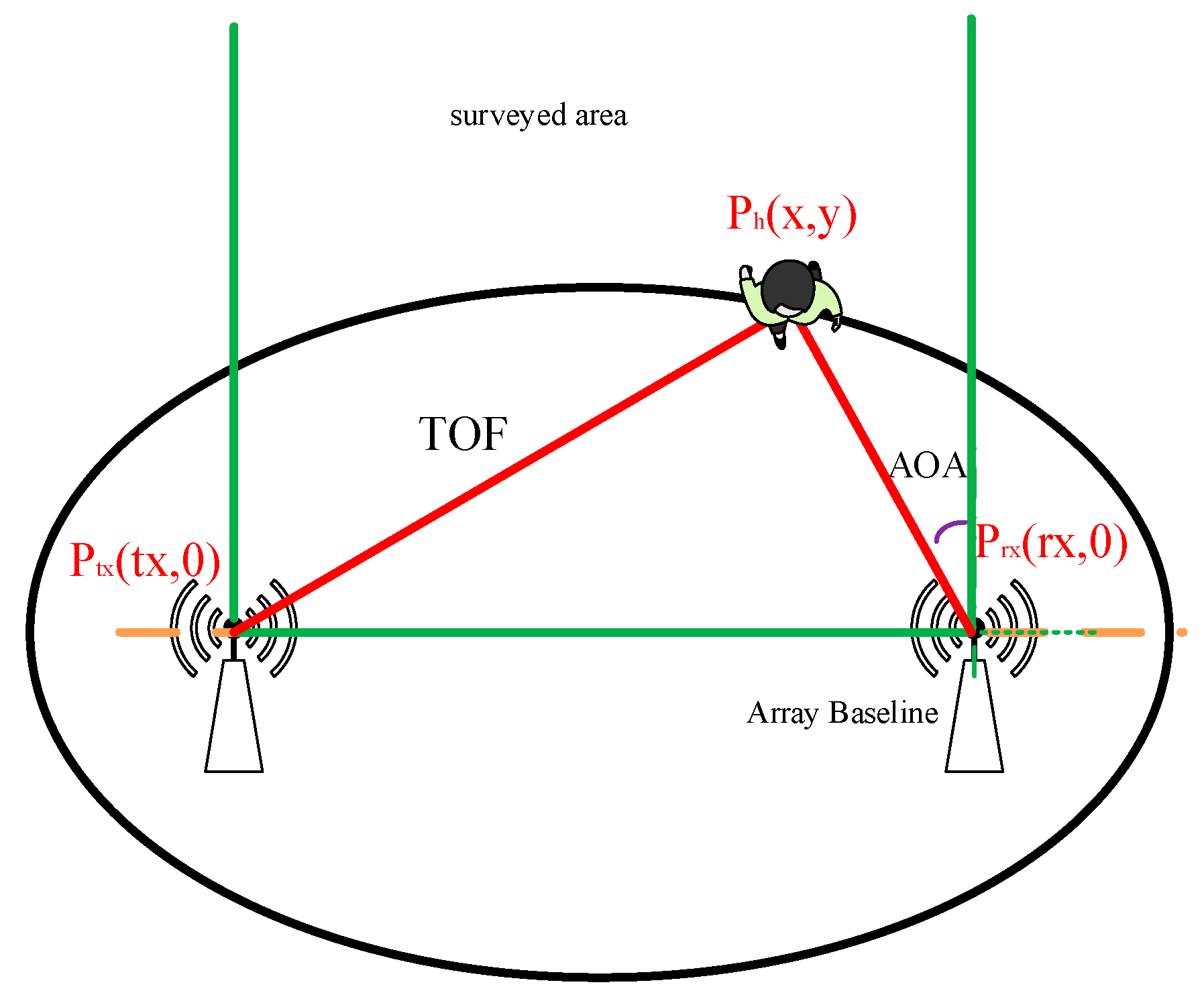
2. Materials and Methods
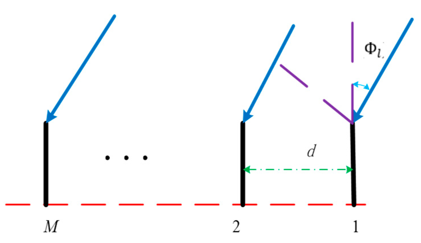
As shown in the previous section, the proposed system involves CSI modeling, phase calibration, static path elimination, a 3D range-adaptive MUSIC algorithm, Kalman filtering, and tracking. The section describes each operation.

2.1. CSI Modeling

WiFi signals propagate and are scattered by any objects they encounter in an indoor environment. Therefore, WiFi signals’ CSI embodies the information about static and dynamic objects (and thus paths) in an environment.
We consider the receiving array of M elements, as shown in Figure 2.
We denote the kth subcarrier signal of the ith packet received by the mth antenna element as h ( i , m , k , t ) . It will contain the signal coming from the static paths due to the stationary objects or from the dynamic paths due to a moving target. The lsth static path signal is denoted as h l s ( i , m , k , t ) and the ldth dynamic path signal as h l d ( i , m , k , t ) . Mathematically, we have:
h ( i , m , k , t ) = l s = 1 L s h l s ( i , m , k , t ) + l d = 1 L d h l d ( i , m , k , t ) + N ( t ) = l s = 1 L s a l s ( i , m , k , t ) e j 2 π f i τ l s ( i , m , k , t ) +         l d = 1 L d a l d ( i , m , k , t ) e j 2 π f i τ l d ( i , m , k , t ) + N ( t )
where Ls represents the total number of static paths, and Ld represents the total number of dynamic paths in the environment. h l s ( i , m , k , t ) represents the kth subcarrier signal of the ith packet received by the mth element from static path ls. h l d ( i , m , k , t ) represents the kth subcarrier signal of the ith packet received by the mth element from dynamic path ld. a l s ( i , m , k , t ) represents the magnitude of the kth subcarrier signal of the ith packet received by the mth element from static path ls. τ l s represents the signal flight time along static path ls. a l d ( i , m , k , t ) represents the magnitude of the kth subcarrier signal of the ith packet received by the mth element from dynamic path ld. τ l d ( i , m , k , t ) represents the flight time along dynamic path ld. N(t) represents noise in the path.
Now, we consider the phase difference between the first subcarrier signal h ( 1 , 1 , 1 , t ) of the first packet received by the first antenna and the kth subcarrier signal h ( i , m , k , t ) of the ith packet received by the mth antenna element. The phase difference is due to three factors: different propagation distances between the elements, the different subcarrier frequencies, and Doppler frequency shifts due to the movement of a target. They are elaborated as follows:
(1)
The phase difference due to the different propagation distances between the elements
It is well known or can be easily inferred from Figure 2 that the phase difference due to the different propagation distances between the mth element and the 1st element is:
φ g = 2 π f k ( m 1 ) d sin ϕ l c   with   l = l s   or   l = l d
where fk is the frequency of the kth subcarrier, d(m − 1) is the extra propagation distance for the mth antenna in reference to that for the first antenna, c is the speed of light, and ϕ l s or ϕ l d are the AOAs of static path ls or dynamic path ld.
As seen, the phase difference (2) between different antennas contains AOA information ϕ l of different paths.
(2)
The phase difference due to the different subcarrier frequencies
Figure 3 shows the schematic diagram of the subcarrier interval. The phase shift between the two subcarrier frequencies received by the same antenna element is φ s ( τ l ) = 2 π Δ f τ l , where Δ f is the frequency difference between the two adjacent subcarriers. For equally spaced OFDM subcarriers, the phase difference between the kth subcarrier and the first subcarrier is
φ s = 2 π Δ f τ l = 2 π Δ f k τ l
where Δ f = Δ f k = ( k 1 ) δ f and δ f is the frequency difference between the adjacent subcarriers.
As seen, the phase difference (3) between different subcarriers contains TOF information τ l .
(3)
The phase difference due to the Doppler frequency shift
If a target or an object is moving, it will incur a Doppler frequency shift, say f D . The phase difference between the ith packet signal and the first packet signal received by an element is:
φ D = 2 π f D ( t i t 1 ) = 2 π v f c ( t i t 1 ) / c
where f D refers to the Doppler frequency shift, f c refers to the central frequency of the packet signal, and Δ t i =   t i t 1 refers to the time difference between the ith packet and the first packet. v is the velocity of the moving target. c is the speed of light.
As seen, the phase difference (4) due to the Doppler effect contains the velocity information v of the moving target.
(4)
The total phase difference between the CSI subcarriers
With (2), (3), and (4), we can find the total phase difference phase between the kth subcarrier h ( i , m , k , t ) of the ith packet received by the mth antenna and the reference subcarrier (which is the first subcarrier signal h ( 1 , 1 , 1 , t ) of the first packet received by the first antenna in our case). The difference can be expressed as:
φ ( i , m , k , t ) = φ g + φ s + φ D = 2 π ( f k ( m 1 ) d sin ϕ l c + Δ f k τ l + f D Δ t i )
As seen, the above phase difference (5) contains the location information of a target. Once it is measured, the location information of a target can be estimated or extracted, including AOA, TOF, and velocity v.
In a real-world situation, imperfect hardware clock synchronization exists and can result in unwanted time offset, frequency shifts, and initial phases, which can cause errors. Therefore, phase calibration is required to remove the errors. In addition, since we are interested in tracking moving targets and dynamic information, we need to remove the static path information, specifically in AOA, TOF, and velocity determination. They are elaborated in the following subsections.

2.2. Phase Calibration and Static Path Elimination

The received analog signal is converted to a digital signal for processing. As a result, a time offset t S F O will be produced; it leads to the undesired phase bias of 2 π f t S F O , which needs to be eliminated. Packet Detection delay (PDD), denoted as t P D D , will also occur when the packet detector processes the signal; the delay in time is presented by phase deviation in the frequency domain. Therefore, the phase errors induced are
2 π f ( t S F O + t P D D ) .
In addition to the two offsets above, the center frequency at the receiving and sending ends may also be out of sync. After subsequent frequency offset compensation, a new center frequency offset (CFO) will be introduced, resulting in phase deviation φ C F O . Therefore, the overall phase offset of the kth subcarrier signal is:
2 π δ f ( k 1 ) ( t S F O + t P D D ) + φ C F O ,
δ f is the frequency difference between adjacent subcarriers.
To remove the above unwanted phase offset or noises, two common phase-calibrated techniques have been developed: the first is the linear fitting algorithm [22,23,27], and the other is the conjugate multiplication of different antenna signals [25,26]. They are applied to pre-process the received signals before the actual estimation algorithms (MUSIC in our case) are applied. In the following paragraphs, we compare the performances of the two different algorithms for location estimation.
The linear fitting algorithm is described in [22,23,27], and the other is the conjugate multiplications of the signals received by different elements; it is described in [25,26]. To see which algorithm is more suitable for the trajectory tracking algorithm, the following experiments are carried out. After the phase calibrations with the two different algorithms, a MUSIC algorithm is applied to estimate AOA and TOF.
Figure 4 shows the AOAs estimated with the linear fitting algorithm for the static and dynamic paths. The black curves are the true AOAs of the moving target. The blue asterisks are the estimated AOAs corresponding to the first peak of the MUSIC power spectrums. The red asterisks are the AOAs corresponding to the second peak point of the power spectrum. They represent the two paths, one being static and the other being dynamic. The AOAs of the static and dynamic paths are indistinguishable when the time is less than 1 s (the abscissa is less than 10). As shown in the red circle in Figure 4, static and dynamic paths are among each other and not distinguishable. One of the reasons for this is that there are only three receiving antennas and the resolution is low.
Figure 5 shows the AOAs estimated with the conjugate multiplication. The black line represents the true AOAs of the moving target. The blue asterisks are the estimated AOAs.
In comparisons of Figure 4 and Figure 5, we can see the conjugate method presents better results than the linear fitting algorithm. In the following subsections, we use the conjugate method.

2.3. The Proposed System with the Three-Dimensional MUSIC Algorithm of Dynamic Step Size

The above work has been limited to the two-dimensional AOA estimations. We now extend it to three-dimensional estimations of AOA, TOF, and Doppler velocities of moving targets with MUSIC algorithms. The specific process of the algorithm is as follows:
It can be seen from Formula (5) that the phase difference of different subcarriers contains TOF information, the phase difference of different antennas contains AOA information, and the phase difference of different times contains Doppler information. CSI data collected within T seconds contain 90 × I packets (I = T × RS, RS is the sampling rate): 90 = 3 (antennas) × 30 (subcarriers)). The AOA and TOF information is included in 90 (row of matrix 90 × I). The speed information is contained in the I of 90 × I.
Because the MUSIC algorithm requires a sufficient number of snapshots, I cannot be always used to estimate Doppler velocity. Therefore, the matrix is reconstructed and sampled for every set of P packets (equivalent to I/P array antennas used to estimate the velocity). The resulting matrix is [90 × (I/P)] × P; P is the number of snapshots, and (90 × (I/P)) is 3 (estimated AOA) × 30 (estimated TOF) × (I/P) (estimated Doppler). The accuracy and resolution of the MUSIC algorithm are directly related to the number of antennas. The number of antennas in this algorithm is 90 × (I/P). However, there are only 30 measured subcarriers in our case, the same as those in the literature [22,27] (2 antennas and 15 subcarriers for each antenna). The superiority of the algorithm in this paper can be seen from the subsequent analysis of the results. The constructed covariance matrix R is as follows:
R = E { l d = 1 L d h l d l d = 1 L d h l d H }
Here, E denotes the expectation. h l d is the CSI time domain signal after removing the static signal. The feature space decomposition of R can be obtained as follows:
R = U s Σ s U s H + U n Σ n U n H
where U s is the signal space of the matrix. U n is the noise space of the matrix. Σ s are the eigenvalues of signal space. Σ n are the eigenvalues of noise space. Let us sort the eigenvalues (eig_matrix). The formula for calculating the decrease ratio is as follows:
d e c _ r a t i o = e i g _ m a t r i x ( i i + 1 ,   i i + 1 )   e i g _ m a t r i x ( i i ,   i i ) ,   ( i i = 1 , 2 , ,   I I )
where II is the total number of rows or columns in the feature space of R. We compute the decrease factors between each adjacent pair of eigenvalues, except the first decrease. We find the largest decrease ratio that occurs between the eigenvalues. Taking the maximum decline rate as the cut-off point, the characteristic space corresponding to the characteristic value is divided into U n and U s . We also need the steering vector in the MUSIC algorithm. The signal’s steering vector of a path with the signal composed of the packet, the subcarrier, and the antenna can be expressed as:
a ( θ l ) = [ 1 , Φ ( τ l ) , , Φ ( τ l ) I 1 antenna 1 , Φ ( θ l ) , , Φ ( θ l ) Φ ( τ l ) I 1 antenna 2 , Φ ( θ l ) ( M 1 ) , , Φ ( τ l ) I 1 Φ ( θ l ) ( M 1 ) antenna M Packet   1 , 1 , Φ ( τ l ) , , Φ ( τ l ) I 1 antenna 1 , Φ ( θ l ) , , Φ ( θ l ) Φ ( τ l ) I 1 antenna 2 , Φ ( θ l ) ( M 1 ) , , Φ ( τ l ) I 1 Φ ( θ l ) ( M 1 ) antenna M Packet   p + 1 , 1 , Φ ( τ l ) , , Φ ( τ l ) I 1 antenna 1 , Φ ( θ l ) , , Φ ( θ l ) Φ ( τ l ) I 1 antenna 3 , Φ ( θ l ) ( M 1 ) , , Φ ( τ l ) I 1 Φ ( θ l ) ( M 1 ) antenna M Packet   ( I P + 1 ) ] T
The steering vector for all multipath paths is
A = [ a ( θ 1 ) , a ( θ 2 ) , , a ( θ l ) , , a ( θ L ) ] T .
Estimates of AOA, TOF, and velocity can be obtained by searching for the peaks of PMUSIC:
P M u s i c = 1 ( A H U n U n H A ) .
The search is full-scale three-dimensional: AOA from −90 degrees to 90 degrees, TOF from −10 ns to 100 ns, and the velocity from −4 m/s to 4 m/s. Without an optimization algorithm, it would take about 10 h to complete a three-dimensional search; such a long computation time is unacceptable.
In this paper, with the consideration that AOA, TOF, and radial velocity information of target motion are usually continuous in adjacent time, a dynamic convolving step search is proposed. The search is carried out within a small range centered at the parameters estimated at the previous time. The search range of AOA depends on the estimated value of AOA at the previous time. More specifically, it is a small range centered on the estimated value of AOA at the previous moment. The search ranges for the TOF and the velocity are similar to that for AOA. With the above search method, the computational time required is reduced from a few hours to tens of seconds. We figured out the running time for both algorithms under the same computer and software platform. The algorithm in this paper is based on the principle that the parameters of human body position are continuous in a short time. The algorithm improves the efficiency by reducing the parameter search range. The original algorithm required 180 × 110 × 80 searches. The improvement only requires 5 × 8 × 12 searches. So, this is about a 3000-fold increase in efficiency.
The above method is very much dependent on the previous estimations. If a previous estimation is wrong, the current estimation can be incorrect. We have conducted another experiment, and the result is shown in Figure 6. In the figure, the purple line is the true AOA, and the colored asterisks are the AOA obtained with the above parametric value that defines the search range. As seen, an error occurred at time 5 s (abscissa 50), resulting in the subsequent incorrect results.
To solve the above problems, the search range needs to be changed adaptively. The first thing we have to do is set up a judging criterion that can identify the starting location of the wrong estimation. Once the location is identified, we can adaptively increase the search range by creating the parametric value. In this paper, the difference between the estimated phase and the original phase is used as the criterion:
ϕ ˜ ( i , k , m , t ) = 2 π ( f k ( m 1 ) d sin ϕ ˜ l c + Δ f k τ ˜ l + f ˜ D Δ t i ) ,
where ϕ ˜ ( i , k , m , t ) is the estimated phase, and τ l ˜ ,   Φ l ˜ , and f D ˜ are the parameters obtained by using the MUSIC algorithm with a fixed parametric value. The estimate deviation var is defined as:
var ( t ) = ϕ ˜ ( i , k , m , t ) ϕ ( i , k , m , t ) .
If var ( t ) T ϕ , we increase the search range and conduct the research.

2.4. Adaptive Kalman Filtering

To further improve the quality of the signals received, we apply the adaptive Kalman filter to filter the signals received.
In general, the Kalman filter’s parameters need to be determined adaptively via continuous trial and error. A Kalman filter with adaptive parameter adjustment is proposed in this paper. The variances in observation noise and state noise can be adjusted adaptively according to the accuracy of the current measured value. The specific process is as follows:
Q 1 ( t ) = a b s ( var ( t ) α )   and
R 1 ( t ) = a b s ( β Q 1 ( t ) ) ,
where Q 1 ( t ) and R 1 ( t ) are the variances in state noise and observation noise, respectively. α and β are the parameters.
The prediction steps of AOA are as follows:
ϕ ˜ l , t ¯ = F 1 ϕ ˜ l , t 1 ,
P ¯ t = F 1 P t 1 F 1 + Q 1 ( t ) ,
where F1 is the state transition matrix. ϕ ˜ l , t 1 is the estimated AOA of path l at time t − 1. ϕ ˜ l , t ¯ is the previously estimated AOA of path l at time t. P ¯ t and P t 1 are the median values of the filter. The updated steps of AOA are as follows:
K 1 = ( P ¯ t H 1 ) i n v ( H 1 P ¯ t H 1 + R 1 ( t ) ) ,
ϕ ˜ l , t = ϕ ˜ l , t ¯ + K 1 ( ϕ l , t H 1 ϕ ˜ l , t ¯ ) ,
P t = ( 1 K 1 H 1 ) P ¯ t .
where K 1 is the filter gain and H1 is the transition matrix from state variables to measurements (observations). inv() is the inverse function.
TOF and velocity estimates are filtered in the same way. The results of the proposed system are shown in Figure 7: it can be seen that the parameter values estimated using the above algorithm are closer to the real purple curve.
The initial estimation is very important for subsequent estimations. In our case, the starting estimation is determined by the center point of the full-range search with stride lengths at multiple times.
The specific algorithm is shown in Algorithm 1, where T is a pre-defined threshold according to experience. The results of the algorithm can be seen in the comparison of Figure 6 and Figure 7.
Algorithm 1: Real-time tracking system algorithm.
In put:  h l d , intalv, intalaoa, intaltof
Output: location
1: Convert h l d matrix;
2: Compute R;
3: Obtained un;
            Dopple: intalv-v:0.2: intalv + v;
            AOA: intalaoa-aoa:2: intalaoa + aoa;
            TOF: intaltof-t:2 e−9: intaltof + t;
4: Use Formula (12) to calculate PMUSIC;
            Find parameters corresponding to the three maximum peaks
5: Take the mean value of the parameters obtained in step 4;
6: Filter Formulas (16)–(22);
7: Substitute result of step 6 into Formula (13) to ˜ ( i ,   k ,   m ) ;
8: plug ˜ ( i ,   k ,   m ) into Formula (14);
            if abs(var) > T,
                    Re-search PMUSIC with the full range
                    Repeat steps 4, 5, and 6, 7, 8
            end
9: Localization by particle filter
Figure 8a–c are the estimated AOA, TOF, and velocity with the proposed system. It can be seen from the results that the variance in the estimated results is smaller than that in Figure 5.

2.5. Trajectory Tracking

As shown in Figure 9, the red line represents the TOF of the target. The purple line represents AOAs with respect to the green coordinates. With the determinations of AOAs and TOFs, a unique position can be determined within the detection area enclosed by the eclipse, which corresponds to the search area.

3. Results

We conducted our experiment with our proposed system and Widar2.0 system for comparisons. The readers can gain a better understanding of the rooms’ layouts and the possible effects of the multipath phenomenon from [26]. It uses one pair of transceiver antennas, a laptop for the receiver, and another laptop for the sender. Every receiving end has three sets of receiving antennas, forming a linear antenna array with the spacing of 0.026 cm (half wavelength) between them. The WiFi transmitter has one antenna. The WiFi signal is channel 165 with a center frequency of 5.825 GHz. Then, the velocity, AOA, TOF estimation error, and trajectory tracking error are analyzed and compared.

3.1. Accuracy of Doppler Velocity Estimation

Figure 10 shows the comparison of the radial velocity accuracy between the proposed system and Widar2.0 in the three environments (classroom, office, and the corridor). The average velocity error of all trajectories in the proposed system in all environments is 0.4527 m/s, and that of Widar2.0 is 0.6574 m/s. Figure 10 shows that the system is not making any velocity errors above 3 m/s, while 70% of the time, the error is less than 1 m/s. The proposed system’s accuracy of velocity estimation is better than Widar2.0. With the proposed system, the system can detect speed information in real time.

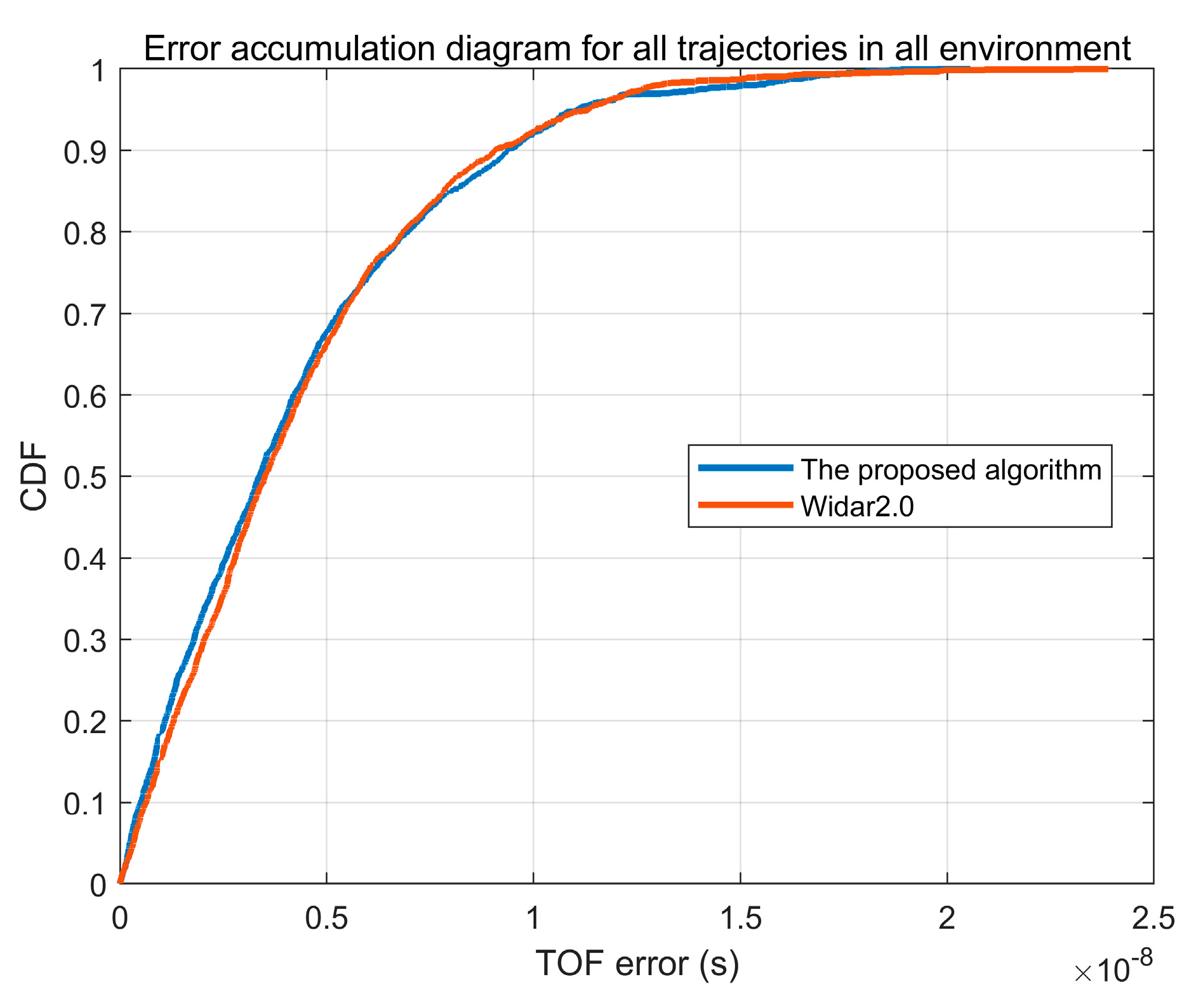
3.2. Accuracy of the TOF Estimation

Figure 11 shows the comparison of TOF accuracy between the proposed system and Widar2.0 in the three environments. The average error of all trajectories in the proposed system in all environments is 3.9550 ns, and the average error of Widar2.0 is 4.0217 ns. The proposed system’s accuracy of TOF estimation is better than Widar2.0. Figure 11 shows that the system is not making any TOF errors above 17 ns, while 70% of the time, the error is less than 5 ns. In addition, the system in this paper can detect TOF information in real time.

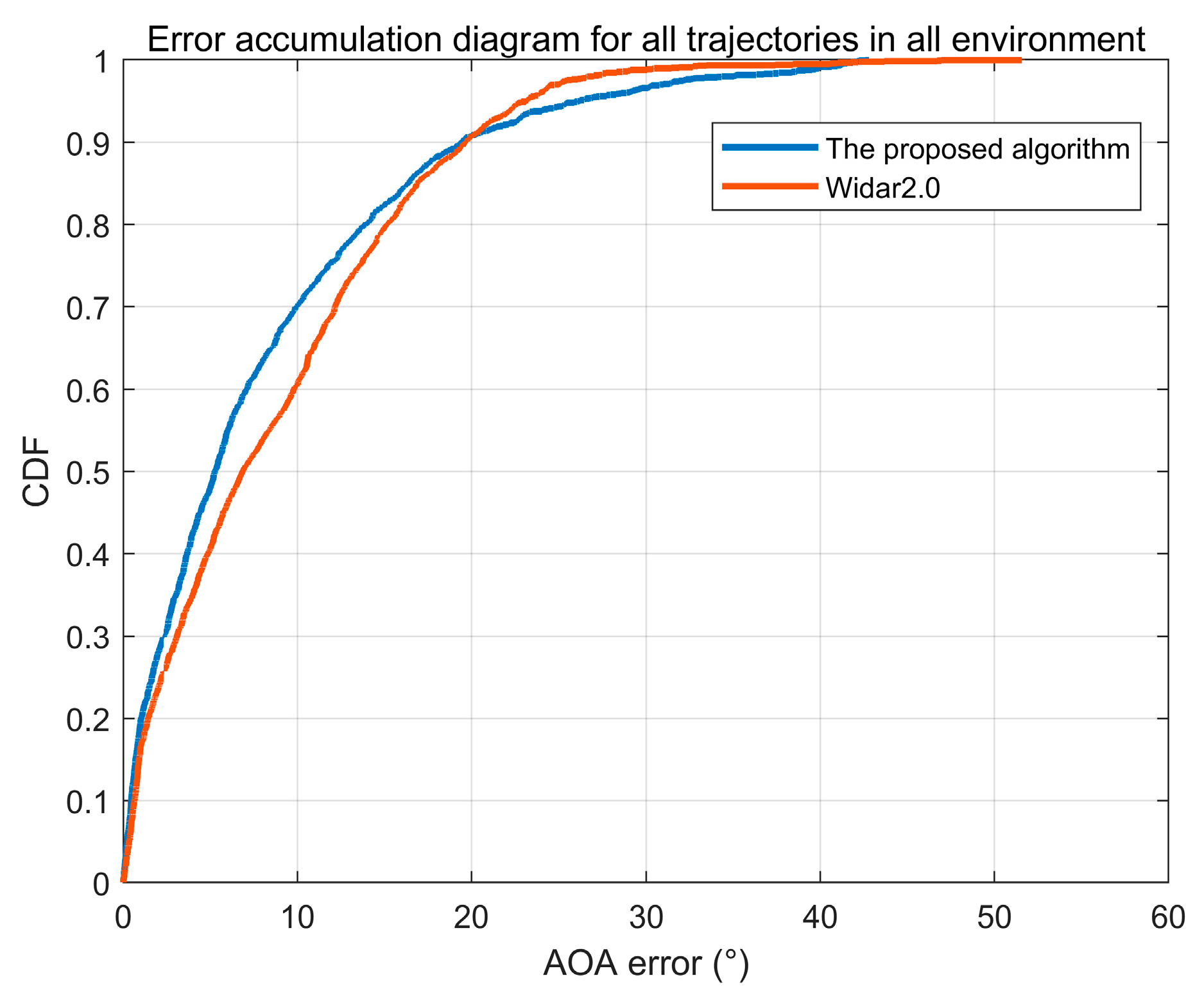
3.3. Accuracy of AOA Estimation

Figure 12 shows the comparison of AOA accuracy between the proposed system and Widar2.0 in the three environments. The average error of all trajectories in the proposed system in all environments is 8.0115°, and the average error of Widar2.0 is 8.734°. The proposed system’s accuracy of AOA estimation is better than Widar2.0. Figure 12 shows that the system does not make any AOA errors above 42°, while 70% of the time, the error is less than 10°. In addition, the proposed system can detect AOA information in real time.

3.4. Estimation of Trajectory Accuracy

The example of location results for the three environments is shown in Figure 13. Figure 13a is for the classroom environment, Figure 13b is for the office environment, and Figure 13c is for the corridor environment. In the narrow corridor environment, the multipath phenomenon is more prominent.
Figure 14 shows the analysis of all the trajectory tracking errors of the proposed system in comparison with Widar2.0. The average error of the proposed system is 0.68 m, and that of Widar2.0 is 0.75 m. The maximum error of this algorithm is greater than Widar2.0. This is because to achieve real-time tracking, the proposed system only uses the information of the previous estimation and the current observation value to determine the final position. Widar2.0 uses the path matching algorithm, Hampel filtering, and smoothing filtering for all time data, so the results are more stable.

4. System Performance

In order to further understand the system performance of the proposed system, we perform analyses with respect to three different affecting factors: environments, data sampling rates, and trajectory shapes.

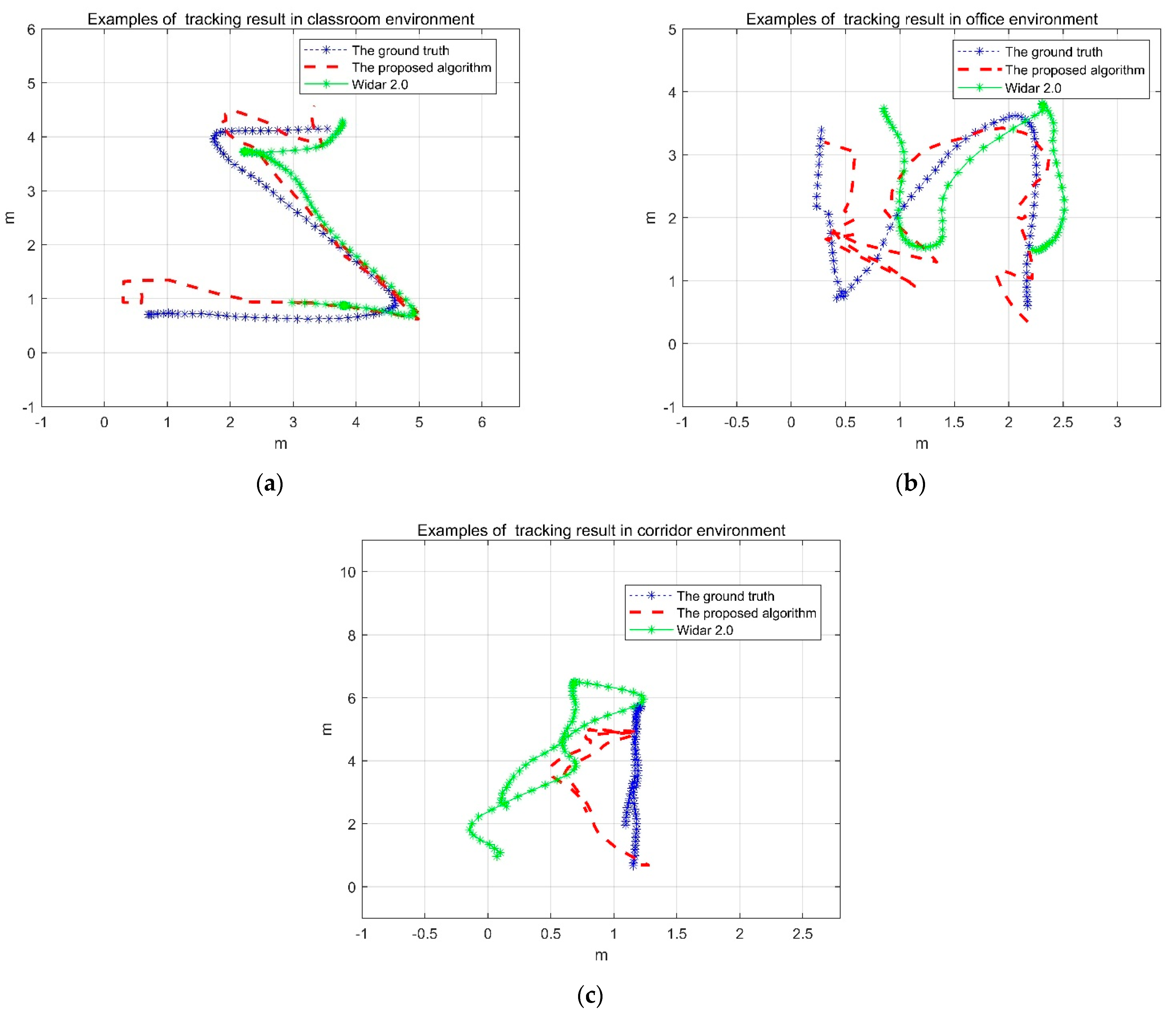
4.1. The Influence of Environments on Tracking Accuracy

In this experiment, we analyze the errors of the three test environments of Widar2.0. Figure 15 is the CDF of the error accumulations of the three environments. The error is greatest in the classroom environment. This is because there are more multipath interferences on the signal, and the two antennas in the classroom are spaced more widely and can detect weaker Doppler speeds. In addition, the error is related to the detection area. The classroom’s detection area is 30 square meters, the hallway is 20 square meters, and the office is 10 square meters. The larger the detection area, the greater the error.

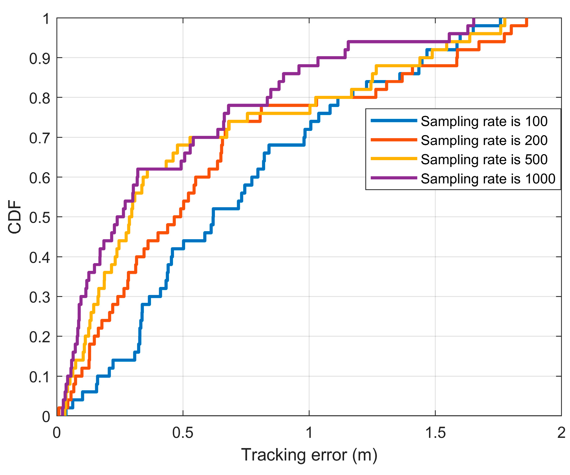
4.2. The Influence of Sampling Rates on Tracking Accuracy

Figure 16 shows the errors at different packet rates: 100/s, 200/s, 500/s, and 1000/s. As the sampling rate decreases, the errors do not change much. The proposed system can still obtain good results at a low sampling rate of 100 packets per second.

4.3. The Influence of the Shapes of Trajectory on Tracking Accuracy

We compared the errors under three different trajectories: Z-shaped, rectangular, and vertical. Figure 17 shows that the overall error of the vertical line is the smallest. This is because when a target moves in a straight line, the TOF information is more continuous, and the results are more accurate. For the Z shape, there will be more information at the turn, so the error is the largest. The errors associated with the rectangle are in between those with the vertical and the Z shape.

5. Conclusions and Discussion

This paper proposes a single-link, real-time location system based on WiFi signals. The system uses a three-dimensional MUSIC algorithm to estimate AOA, TOF, and radial velocity information. By applying the adaptive determination of the search range, the proposed system avoids a full three-dimensional search, reducing the computation time from about ten hours to tens of seconds. In comparison with Widar2.0, the proposed system does not need to perform path matching and smoothing filtering. Rather, the proposed system makes the estimations based on those of the previous ones at the previous moments. The average tracking error is 0.68 m, which is better than those of the existing systems. At present, the algorithm in this paper can only track the motion of one person. For the case of multiple people moving at the same time, the estimated parameters will be superimposed and cannot be distinguished, and the trajectory cannot be accurately tracked. Multi-person tracking based on Wi-Fi is one of the future research directions.

Author Contributions

Conceptualization, L.-P.T. and L.-Q.C.; methodology, L.-P.T.; software, L.-P.T.; validation, L.-P.T., Z.C. and Z.-M.X.; investigation, L.-P.T.; resources, Z.-M.X.; data curation, L.-Q.C.; writing—original draft preparation, Z.-M.X.; writing—review and editing, L.-P.T.; visualization, L.-P.T.; supervision, L.-Q.C.; project administration, Z.C.; funding acquisition, Z.C. All authors have read and agreed to the published version of the manuscript.

Funding

This work was supported in part by the National Natural Science Foundation of China (NSFC) 62071125, National Key Research and Development Program of China under Grant 2022YFE0115500, Natural Science Foundation of Fujian Province under Grant 2021J01581, Industry-University-Research Collaboration Project of Fujian Province under Grant 2022H6018, 2023 Fujian Chuanzheng Communications College University-level Science and Education Development Fund Project (Doctoral research launch special) #20230101, 2022 Annual Young and Middle-aged Teachers Education Research Project (Science and Technology) of Fujian Province #JAT-220543, and Fuzhou University under Scientific Research Project #GXRC-18074.

Institutional Review Board Statement

Not applicable.

Informed Consent Statement

Informed consent was obtained from all subjects involved in the study.

Data Availability Statement

Not applicable.

Conflicts of Interest

The authors declare no conflict of interest.

References

  1. Filippoupolitis, A.; Oliff, W.; Loukas, G. Bluetooth Low Energy Based Occupancy Detection for Emergency Management. In Proceedings of the 2016 15th International Conference on Ubiquitous Computing and Communications and 2016 International Symposium on Cyberspace and Security (IUCC-CSS), Granada, Spain, 14–16 December 2016; pp. 31–38. [Google Scholar]
  2. Tekler, Z.D.; Low, R.; Yuen, C.; Blessing, L. Plug-Mate: An IoT-based occupancy-driven plug load management system in smart buildings. Build. Environ. 2022, 223, 109472. [Google Scholar] [CrossRef]
  3. Balaji, B.; Jian, X.; Nwokafor, A.; Gupta, R.; Agarwal, Y. Sentinel: Occupancy based HVAC actuation using existing WiFi infrastructure within commercial buildings. In Proceedings of the 11th ACM Conference on Embedded Networked Sensor Systems, Roma, Italy, 11–15 November 2013; ACM: New York, NY, USA, 2013. [Google Scholar]
  4. Tekler, Z.D.; Chong, A. Occupancy prediction using deep learning approaches across multiple space types: A minimum sensing strategy. Build. Environ. 2022, 226, 109689. [Google Scholar] [CrossRef]
  5. Liu, S.; Jiang, Y.; Striegel, A. Face-to-Face Proximity Estimation Using Bluetooth on Smartphones. IEEE Trans. Mob. Comput. 2014, 13, 811–823. [Google Scholar] [CrossRef]
  6. Zhao, X.; Xiao, Z.; Markham, A.; Trigoni, N.; Ren, Y. Does BTLE measure up against WiFi? A comparison of indoor location performance. In Proceedings of the European Wireless 2014; 20th European Wireless Conference, Barcelona, Spain, 14–16 May 2014; VDE: Offenbach am Main, Germany, 2014. [Google Scholar]
  7. Tekler, Z.D.; Low, R.; Gunay, B.; Andersen, R.K.; Blessing, L. A Scalable Bluetooth Low Energy Approach to Identify Occupancy Patterns and Profiles in Office Spaces. Build. Environ. 2020, 171, 106681. [Google Scholar] [CrossRef]
  8. Zheng, S.; Purohit, A.; De Wagter, P.; Brinster, I.; Hamm, C.; Zhang, P. PANDAA: Physical arrangement detection of networked devices through ambient-sound awareness. In Proceedings of the Ubiquitous Computing, International Conference, Ubicomp, Beijing, China, 17–19 September 2011. [Google Scholar]
  9. Huang, W.; Xiong, Y.; Li, X.-Y.; Lin, H.; Yang, P.; Liu, Y. Shake and walk: Acoustic direction finding and fine-grained indoor localization using smartphones. In Proceedings of the IEEE Infocom 2014—IEEE Conference on Computer Communications, Toronto, ON, Canada, 27 April—2 May 2014. [Google Scholar]
  10. Mohammadmoradi, H.; Heydariaan, M.; Gnawali, O.; Kim, K. UWB-Based Single-Anchor Indoor Localization Using Reflected Multipath Components. In Proceedings of the International Conference on Computing, Networking and Communications (ICNC), Honolulu, HI, USA, 18–21 February 2019; IEEE: Piscataway, NJ, USA, 2019. [Google Scholar]
  11. Wang, C.; Xu, A.; Kuang, J.; Sui, X.; Hao, Y.; Niu, X. A High-Accuracy Indoor Localization System and Applications Based on Tightly Coupled UWB/INS/Floor Map Integration. IEEE Sens. J. 2021, 21, 18166–18177. [Google Scholar] [CrossRef]
  12. Jin, G.Y.; Lu, X.Y.; Park, M.S. An Indoor Localization Mechanism Using Active RFID Tag. In Proceedings of the IEEE International Conference on Sensor Networks, Ubiquitous, and Trustworthy Computing, Taichung, Taiwan, 5–7 June 2006; IEEE: Piscataway, NJ, USA, 2006. [Google Scholar]
  13. Colin, E. Indoor performance analysis of LF-RFID based positioning system: Comparison with UHF-RFID and UWB. In Proceedings of the International Conference on Indoor Positioning & Indoor Navigation, Taichung, Taiwan, 5–7 June 2006; IEEE: Piscataway, NJ, USA, 2017. [Google Scholar]
  14. Chen, R.; Huang, X.; Zhou, Y.; Hui, Y.; Cheng, N. UHF-RFID-Based Real-Time Vehicle Localization in GPS-Less Environments. IEEE Trans. Intell. Transp. Syst. 2021, 23, 9286–9293. [Google Scholar] [CrossRef]
  15. Zhang, L.; Gao, Q.; Ma, X.; Wang, J.; Yang, T.; Wang, H. DeFi: Robust Training-Free Device-Free Wireless Localization with WiFi. IEEE Trans. Veh. Technol. 2018, 67, 8822–8831. [Google Scholar] [CrossRef]
  16. Zheng, Y.; Sheng, M.; Liu, J.; Li, J. OpArray: Exploiting Array Orientation for Accurate Indoor Localization. IEEE Trans. Commun. 2019, 67, 847–858. [Google Scholar] [CrossRef]
  17. Kumar, S.; Kumar, S.; Katabi, D. Decimeter-Level Localization with a Single WiFi Access Point; USENIX Association: Berkeley, CA, USA, 2016. [Google Scholar]
  18. Shu, Y.; Huang, Y.; Zhang, J.; Coué, P.; Cheng, P.; Chen, J.; Shin, K.G. Gradient-Based Fingerprinting for Indoor Localization and Tracking. IEEE Trans. Ind. Electron. 2016, 63, 2424–2433. [Google Scholar] [CrossRef]
  19. Wang, X.; Gao, L.; Mao, S.; Pandey, S. CSI-Based Fingerprinting for Indoor Localization: A Deep Learning Approach. IEEE Trans. Veh. Technol. 2017, 66, 763–776. [Google Scholar] [CrossRef]
  20. Sun, W.; Xue, M.; Yu, H.; Tang, H.; Lin, A. Augmentation of Fingerprints for Indoor WiFi Localization Based on Gaussian Process Regression. IEEE Trans. Veh. Technol. 2018, 67, 10896–10905. [Google Scholar] [CrossRef]
  21. Shi, S.; Sigg, S.; Chen, L.; Ji, Y. Accurate Location Tracking From CSI-Based Passive Device-Free Probabilistic Fingerprinting. IEEE Trans. Veh. Technol. 2018, 67, 5217–5230. [Google Scholar] [CrossRef]
  22. Kotaru, M.; Joshi, K.; Bharadia, D.; Katti, S. Spotfi: Decimeter level localization using WiFi. In Proceedings of the ACM SIGCOMM, London, UK, 17–21 August 2015. [Google Scholar]
  23. Xiang, L.; Li, S.; Zhang, D.; Xiong, J.; Wang, Y.; Mei, H. Dynamic-MUSIC: Accurate device-free indoor localization. In Proceedings of the ACM International Joint Conference ACM, Heidelberg, Germany, 12–16 September 2016. [Google Scholar]
  24. Qian, K.; Wu, C.; Yang, Z.; Liu, Y.; Jamieson, K. Widar: Decimeter-Level Passive Tracking via Velocity Monitoring with Commodity WiFi. In Proceedings of the ACM MobiHoc 2017, Chennai, India, 10–14 July 2017. [Google Scholar]
  25. Li, X.; Zhang, D.; Lv, Q.; Xiong, J.; Li, S.; Zhang, Y.; Mei, H. IndoTrack: Device-Free Indoor Human Tracking with Commodity WiFi. In Proceedings of the ACM IMWUT 2017, Maui, HI, USA, 3 September 2017. [Google Scholar]
  26. Qian, K.; Wu, C.; Zhang, Y.; Zhang, G.; Yang, Z.; Liu, Y. Widar2.0: Passive Human Tracking with a Single WiFi Link. In Proceedings of the 16th Annual International Conference, Munich, Germany, 10–15 June 2018. [Google Scholar]
  27. Zhang, L.; Wang, H. Device-Free Tracking via Joint Velocity and AOA Estimation with Commodity WiFi. IEEE Sens. J. 2019, 19, 10662–10673. [Google Scholar] [CrossRef]
Figure 1. The proposed system.
Remotesensing 15 02461 g001
Figure 2. Array signal diagram.
Remotesensing 15 02461 g002
Figure 3. The interval between two adjacent subcarriers.
Remotesensing 15 02461 g003
Figure 4. The AOAs’ estimation using the linear fitting algorithm.
Remotesensing 15 02461 g004
Figure 5. The AOAs’ estimation with the conjugate multiplication of the signals received at different antennas.
Remotesensing 15 02461 g005
Figure 6. The incorrect AOA estimation due to the erroneous estimation at t = 5 s.
Remotesensing 15 02461 g006
Figure 7. Conjugate multiplication for different antenna signals before AOA estimation with the Kalman filter.
Remotesensing 15 02461 g007
Figure 8. The estimation results of AOA, TOF, and the velocity with MUSIC. (a) The AOA estimated with Algorithm 1; (b) the TOF estimated with Algorithm 1; (c) the velocity estimated with Algorithm 1.
Remotesensing 15 02461 g008
Figure 9. The location and tracking diagram.
Remotesensing 15 02461 g009
Figure 10. The cumulative distribution function (CDF) of the velocity errors with different algorithms.
Remotesensing 15 02461 g010
Figure 11. The CDF of the TOF errors with different algorithms.
Remotesensing 15 02461 g011
Figure 12. The CDF of the AOA errors with different algorithms.
Remotesensing 15 02461 g012
Figure 13. The tracking results for different shapes of trajectory. (a) The ‘Z’-shaped trajectory in the classroom; (b) the ‘Z’-shaped trajectory in the office; (c) the line trajectory in the corridor.
Remotesensing 15 02461 g013
Figure 14. The CDF of the tracking errors with different algorithms.
Remotesensing 15 02461 g014
Figure 15. The CDF of tracking errors versus different environments.
Remotesensing 15 02461 g015
Figure 16. The CDF of tracking errors versus different sampling rates.
Remotesensing 15 02461 g016
Figure 17. The CDF of AOA errors versus different environments.
Remotesensing 15 02461 g017
Disclaimer/Publisher’s Note: The statements, opinions and data contained in all publications are solely those of the individual author(s) and contributor(s) and not of MDPI and/or the editor(s). MDPI and/or the editor(s) disclaim responsibility for any injury to people or property resulting from any ideas, methods, instructions or products referred to in the content.

