Article

Disentangling the Key Drivers of Ecosystem Water-Use Efficiency in China’s Subtropical Forests Using an Improved Remote-Sensing-Driven Analytical Model

1
Department of Physical Geography, Resources and Environment, School of Geography and Planning, Sun Yat-sen University, Guangzhou 510275, China
2
State Key Laboratory of Desert and Oasis Ecology, Xinjiang Institute of Ecology and Geography, Chinese Academy of Sciences, Urumqi 830011, China
3
Key Laboratory of Water Cycle and Related Land Surface Processes, Institute of Geographic Sciences and Natural Resources Research, Chinese Academy of Sciences, Beijing 100101, China
4
University of Chinese Academy of Sciences, Beijing 100049, China
*
Author to whom correspondence should be addressed.
Remote Sens. 2023, 15(9), 2441; https://doi.org/10.3390/rs15092441
Submission received: 21 March 2023 / Revised: 23 April 2023 / Accepted: 3 May 2023 / Published: 6 May 2023
(This article belongs to the Section Forest Remote Sensing)

Abstract

:
The subtropical forests in China play a pivotal part in the global and regional carbon–water cycle and in regulating the climate. Ecosystem water-use efficiency (WUE) is a crucial index for understanding the trade-off between ecosystem carbon gain and water consumption. However, the underlying mechanisms of the WUE in forest ecosystems, especially the different subtropical forests, have remained unclear. In this paper, we developed a simple framework for estimating forest WUE and revealing the underlying mechanisms of forest WUE changes via a series of numerical experiments. Validated by measured WUE, the simulated WUE from our developed WUE framework showed a good performance. In addition, we found that the subtropical forest WUE experienced a significant increasing trend during 2001–2018, especially in evergreen and deciduous broadleaf forests where the increasing rate was greatest (0.027 gC kg−1 H2O year−1, p < 0.001). Further analysis indicated that the atmospheric CO2 concentration and vapor pressure deficits (VPD), rather than leaf area index (LAI), were the dominant drivers leading to the subtropical forest WUE changes. When summed for the whole subtropical forests, CO2 and VPD had an almost equal spatial impact on annual WUE change trends and accounted for 45.3% and 49.1% of the whole study area, respectively. This suggests that future forest management aiming to increase forest carbon uptake and protect water resources needs to pay more attention to the long-term impacts of climate change on forest WUE.

1. Introduction

WUE is defined as carbon assimilation per unit of water loss and is a prominent pointer for understanding vegetation carbon–water coupling between photosynthesis and transpiration [1,2]. The ecosystem WUE is expressed as the ratio of gross primary productivity (GPP) to evapotranspiration (ET) [3]. Generally, vegetation returns water vapor to the atmosphere through transpiration, which profoundly influences the regional climate and water yield or runoff [4,5]. Consequently, quantifying the variations in WUE over space and time and revealing its driving mechanisms is essential for comprehending the vegetation carbon–water interactions, predicting and adapting to future climate change [5,6,7], and providing valuable guidance for policy makers in water resources’ management [4,8].
As one of the major terrestrial ecosystems, forest ecosystems, which cover about 30% of the land area [9], are one of the largest conduits for transferring carbon from the atmosphere to the terrestrial ecosystems through photosynthesis [10,11] and reformulating the global or regional climate via water consumption of transpiration [5,12,13]. The Chinese subtropical forest ecosystems, with an area of nearly 1.4 × 10⁶ km2, are an extremely important component of the global forest ecosystems and are hence crucial to the global carbon cycle and regional climate change. Moreover, the subtropical region is one of the most developed areas in China, with over 8% of the world’s population, and the forests in this region can provide important ecosystem services for human beings, such as water resources, carbon sequestration, oxygen production and timber [14,15].
During the past two decades, a series of nationwide vegetation restoration programs related to subtropical forest ecosystems were implemented by the China’s central and district governments to prevent land degradation and mitigate climate change, such as the Grain for Green Program (GGP, launched in 2000), the Yangtze and Pearl River Basin Shelterbelt programs, and the Natural Forest Protection Project (NFPP, launched in 1998) [16]. Evidence from the remotely sensed observations and nationwide field samplings showed an increase in vegetation coverage and greening in southern China [17,18,19]. The changed land surface properties such as the LAI have profoundly affected the available water-energy allocation [4]. As a consequence, the balance between carbon uptake and water consumption (i.e., WUE) has varied with vegetation restoration. In addition, climate change also changed dramatically over the past few decades; the temperature (TEM) in this region has increased by more than 1.0 °C, which exceeds the global average [20]. The precipitation (PRE) shows obvious spatial heterogeneity due to the complex topography and plant types [21]. Therefore, the forest WUE in this region is significantly regulated by changes in temperature and precipitation over space and time. The VPD, as another key driver of the ecosystem WUE, also influences the WUE at different spatiotemporal scales [22].
Moreover, with the rapid economic development and large trace gas emissions (e.g., CO2), not only has the annual mean atmospheric CO2 concentration in China reached new high levels (e.g., 407 ppm in 2017) [23], but air pollution in this region has been reported in the last two decades, which, in turn, affects the solar net radiation, thereby impacting the forest WUE. A previous study reported that the rising CO2 concentration enhanced the plant photosynthetic rates and thereby increased the WUE [24]. As China’s subtropical forest WUE has experienced unprecedented variations caused by multiple factors, it is crucial to elucidate how subtropical forest WUE varies and what the dominant drivers are over space and time. Many studies have explored the spatial–temporal pattern and mechanisms of forest WUE changes at the global scale [3,6,25], regional scale [26,27,28,29,30], and in the south of China [31,32]. Despite substantial efforts, conclusions regarding the drivers of changes in forest WUE remain inconsistent. For example, at the global scale, many previous studies have suggested that the increasing CO2 concentration was the main driving factor for the increase in global WUE [1,6], while there were also studies [5,33] that challenge this hypothesis. At the regional scale, Ding et al. [32] estimated the effects and implications of ecological restoration projects on ecosystem WUE in the karst region of Southwest China and reported a significant upward trend in WUE and suggested that ecological restoration projects were the main driver of the WUE increase. In the karst areas of southern China, Xiao et al. [34] indicated that the WUE showed an insignificant decreasing trend, and the precipitation was the dominant driver of the WUE changes. In addition, most studies treated different forests as a single forest type; thus, the relative impacts of different factors on forest WUE changes in specific forest types remain unclear, particularly in subtropical forest ecosystems.
Methodologically, different techniques have been used to estimate vegetation WUE and to unravel its drivers over multiple spatiotemporal scales. The flux tower can offer reliable carbon–water flux observations for estimating WUE in forest ecosystems, while field measurements of WUE by flux towers are scarce in the Chinese subtropical forest region [35]. Moreover, the footprint of a flux tower is limited from a few kilometers in the best case, which limits our understanding of forest WUE and its driving factors over large spatial scales [35]. Additionally, methods based on statistics and modelling were frequently utilized to understand the WUE variations and their drivers. For example, previous studies used model-simulated (e.g., light utilization efficiency (LUE) model) or remote-sensing-derived GPP and ET to calculate the WUE, and then traditional statistical or regression methods were adopted to explore the drivers of WUE dynamics [8,26,36]. However, the estimated WUE could involve some uncertainty and ignore the photosynthesis–transpiration coupling due to using the independent GPP and ET data [3]. Moreover, the correlation does not necessarily imply causality, which can lead to biased results and conclusions due to spurious correlations [7]. Process-based models are by far one of the most popular methods for estimating WUE [4,7]. Process-based models can explicitly represent the biophysical processes in vegetation and their interaction with the environment, which is regarded as the better tool for understanding the driving mechanisms of WUE changes. Nevertheless, process-based models usually have a complex model structure and require more detailed and strict inputs, as well as pre-calibrated parameters based on the field measurements, which may hinder their application in data-scarce regions, especially in the subtropical regions of China where only a few flux observations are available.
Recently, the analytical WUE model [6] was widely used to simulate and diagnose the driving mechanism of WUE changes [6,37,38]. The analytical WUE model has the advantages of a solid biophysical foundation and a simple model structure. It requires few parameters and model inputs (e.g., only a few remote sensing data) [6,37,39]. Moreover, in contrast to the traditional ecosystem WUE model based on the ratio of GPP and ET [1,3,26], the analytical WUE model directly upscales WUE from the leaves to the ecosystem without pre-estimating GPP, thus tremendously reducing the uncertainty [6,38]. Therefore, this method has huge potential to simulate the subtropical forest WUE and investigate its mechanisms. The model, however, still needs further improvement because of its limitations in detecting some important driving mechanisms of forest WUE changes.
In this study, the analytical WUE model was first modified, and further used to simulate the spatiotemporal variations in the WUE of different subtropical forests. The mechanisms across subtropical forest region were further explored using a range of modeling experiments. The purpose of this paper is to address the following questions: (1) What is the spatial–temporal pattern of the WUE of the Chinese subtropical forests? (2) How has the annual WUE of different subtropical forests varied during the past two decades? (3) What are the dominant drivers of annual WUE change trends in different subtropical forests? The results of this study may offer valuable information for policy makers in forest and water resources’ management.

2. Materials and Methods

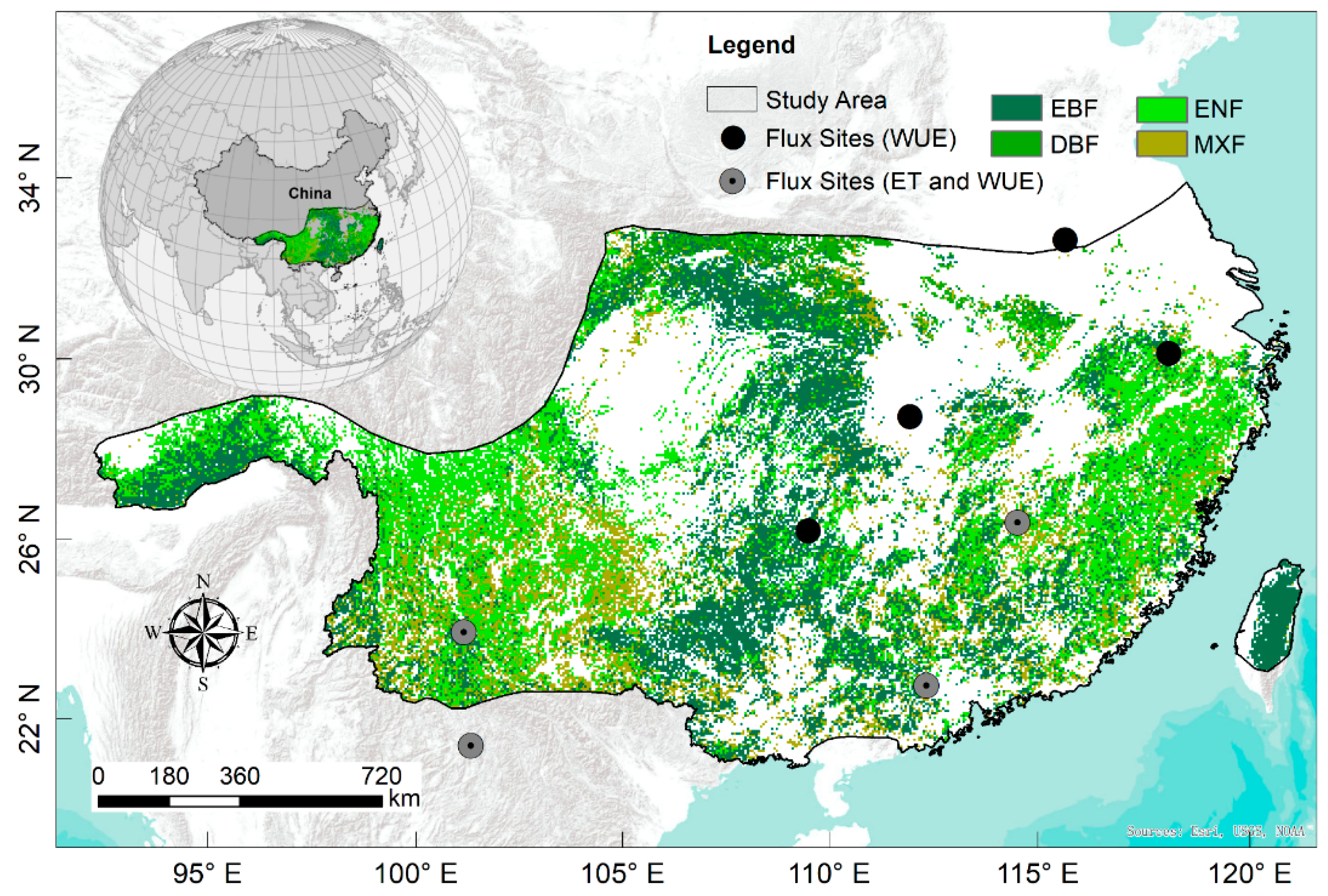
2.1. Study Area Description

In this study, we focus on the subtropical forests [40,41] situated in the south of China, which can be demarcated by coordinates 21.33–33.91°N and 91.39–122.49°E, with a coverage of nearly 1.4 × 10⁶ km2. This region has a typical subtropical monsoon climate. The average annual temperature is about 15.5 °C. The annual precipitation is mainly concentrated in the growing season and shows great spatial heterogeneity, ranging from more than 2000 mm (south) to 800 mm (north). Due to its special climate conditions and geographical position compared with regions at the same latitude, this region has formed unique subtropical forest ecosystems, which are an important part of the global forests [42]. The major forest types in subtropical China include evergreen broad-leaved forest (EBF), evergreen coniferous forest (ENF), deciduous broad-leaved forest (DBF), and mixed forest (MXF) (Figure 1).

2.2. Model Description and Improvement

2.2.1. The Analytical WUE Model

The analytical WUE model [6] in our study was adopted to simulate the annual subtropical forest WUE at a resolution of 0.05° and to unravel its drivers at the annual scale. The ecosystem WUE is expressed as ecosystem carbon assimilation (i.e., GPP) per unit of ecosystem water consumption through evapotranspiration (ET), expressed as follows:
W U E = G P P E T
In Equation (1), the ET includes the following three components:
E T = E t + E i + E s
where E t is transpiration, which links carbon assimilation and water vapor loss via leaf stomata. E i and E s are interception evaporation and soil evaporation, respectively. During the growing season, the GPP and ET are above zero, as suggested by Cheng et al. [6]. Therefore, Equation (1) can be rephrased as three terms:
W U E = G P P E T = G P P E t × E t E t + E s × ( 1 E i E T )
In Equation (3), the first term is the transpiration WUE; the second term represents the partitioning between E t and E s during the carbon uptake period; the third term is determined by the ratio of E i to ET. As indicated by the previous studies [6,43], the leaf WUE ( W U E L ) is independent of the growth environment, and thus W U E L can be directly upscaled to the canopy transpiration WUE by linking CO2 concentration ( C a ), air pressure ( p a ), and VPD. Therefore, G P P / E t in Equation (3) can be approximated by W U E L as follows:
G P P E t = A d t T d t W U E L = A T = C a p a 1.6 × V P D + g 1 V P D
where A denotes the leaf net photosynthetic carbon assimilation rate (μmol (CO2) m−2 s−1); T represents the leaf transpiration rate (μmol (H2O) m−2 s−1); C a is the ambient atmospheric CO2 concentration (µmol(CO2)/mol (air)); VPD and p a , respectively, represent the vapor pressure deficit (kPa) and air pressure (kPa); g 1 is an empirical parameter from the Ball stomatal conductance model (kPa0.5) (Ball et al., 1987), which was used in the WUE model for different land cover types and detailed in Cheng et al. [6]. For the second term in Equation (3), the E t E t + E s can be estimated by Beer’s Law [44]:
E t E t + E s = 1 e x p ( k L )
where the L denotes the leaf area index (LAI) (m2/m2); the k (unitless) is the extinction coefficient of radiation (k = 0.6) [6]. Eventually, the expression of the analytical WUE model is as follows.
W U E = C a p a 1.6 × V P D + g 1 V P D × 1 e x p ( k L ) × ( 1 f E i )
where f E i is the ratio of E i to ET ( E i / E T ).
However, the original analytical WUE model, as shown in Equation (6), is mainly determined by the five controlling factors, namely the C a , p a , VPD, L , and f E i , especially the f E i , calculated based on the published global E i and E T data sets in the original analytical WUE model [6]. Some key drivers, such as precipitation, temperature, net radiation (RN), VPD, and LAI, can also significantly affect E i and E T , thereby influence forest W U E [6,37,38,39]. Therefore, ignoring these drivers may hinder our understanding of the real mechanisms of WUE changes when using the original analytical WUE model. In this study, we attempt to incorporate the Priestley–Taylor Jet Propulsion Laboratory (PT-JPL) model [45] into the original analytical WUE model and to estimate the f E i . Here, we used the PT-JPL model because it not only has the merits of a high-efficiency model structure and high-accuracy estimation of ET and its components ( E t , E i , a n d   E s ), but also considers different physical processes with interactions of the key biotic (i.e., LAI) and environmental factors (e.g., temperature, net radiation, VPD) [45]. Therefore, we can adopt the coupled analytical WUE model to diagnose the effects of different driving forces on WUE change trends [39].

2.2.2. The PT-JPL Model

The PT-JPL model was developed by Fisher et al. [43], and has been adopted to estimate the total ET and three parts of ET, as in Equation (2). In the PT-JPL model, the calculations of the E t   a n d   E s can be shown as follows:
E t = 1 f w e t f g f t f m α + γ R n c
E s = 1 f w e t + f s m 1 f w e t α + γ ( R n s G )
where f w e t is the relative surface wetness (unitless), f g is the green canopy fraction (unitless), f t is the plant temperature constraint (unitless), f m is the plant moisture constraint (unitless), and f s m is the soil moisture constraint (unitless); R n c and R n s , respectively, denote the net radiation to the canopy (W/m2) and the soil (W/m2). G denotes the ground heat flux (W/m2), which can be neglected on a monthly or yearly scale [46,47,48]. The Priestley–Taylor coefficient ( α ) was set as a constant value of 0.8 for forests [47], denotes the slope of the saturated vapor pressure curve (kPa/°C), and γ represents the psychrometric constant (kPa/°C). The calculations of the f w e t , f g , f t , f m , f s m , R n c , and R n s can be found in Table S2 and the previous studies [45,49].
In the PT-JPL model, the E i is generally evaluated by E i = f w e t × α × / ( + γ ) × R n c , which mainly depends on the R n c and relative humidity (RH). However, only considering the R n c and RH may ignore the effect of precipitation on E i , especially in the subtropical forests with dense trees, which have a strong interception and affect the precipitation reaching the ground, influencing the total ET. Moreover, the original E i equation in the PT-JPL model means that E i will occur as long as the RH is greater than 70%, even without precipitation [45]. This assumption may be unsuitable for the humid subtropical region because RH and precipitation are usually uncorrelated, particularly in a humid region such as China’s subtropics, where the RH almost exceeds 70% during the year, but not necessarily with precipitation. Therefore, the original equation in the PT-JPL model may significantly overestimate the E i , as reported by previous studies [50,51], especially in subtropical regions of China, by up to three-fold [38,52]. Therefore, in this study, we adopted the modified Gash model [53,54] to replace the original equations in the PT-JPL model and calculate the E i . Meanwhile, we also compared the E i calculated by the original equation in the PT-JPL model and the modified Gash model, with the other two E i products (i.e., the GLEMA E i and PML-V2 E i ), further confirming that the overestimation of E i in the original PT-JPL model (see Figure S1). The key equations used in the modified Gash model for E i estimation are as follows (Equations (9) and (10)).
E i = f v × P ,   if   P < P w e t f v P w e t + f E R × P P w e t ,   if   P P w e t
with
P w e t = ln 1 f E R f v × S v f E R , S v = S l × L A I , f E R = f v × F 0
where P and P w e t are the daily precipitation (mm/day) and the reference threshold rainfall amount if the canopy is wet (mm/day); f v denotes the fractional area covered by intercepting leaves (unitless), which can be calculated by f v = 1 e x p ( 0.2     L A I ) ; f E R denotes the ratio of average evaporation rate over average precipitation intensity storms (unitless); S v represents the canopy rainfall storage capacity (mm/day); S l (mm) is the water storage capacity per unit leaf; F 0 is the specific ratio of average evaporation rate over average rainfall intensity during storms per unit canopy cover (unitless). In this study, the key parameters of S l and F 0 referred to the study of Zhang et al. [55]. The performance of the modified PT-JPL model (PT-JPLmod) will be validated by measured ET, and the PT-JPLmod will also be compared to the original PT-JPL model (PT-JPLraw) when simulating ET.
Firstly, we use the improved PT-JPL model to calculate ET and E i , where E i is calculated using the improved Gash model. It is worth noting that we do not directly use the Gash model to calculate E i in the analytical WUE model and further simulate the WUE, because E i in this study is also used to calculate ET, thereby affecting the total ET. Then, we use the ratio of E i to ET to calculate f E i (i.e., f E i = E i / E T ) in the original analytical WUE model. Eventually, the modified analytical WUE model is generated, as shown in Figure 2. The simulated WUE was first validated by the measured WUE, and the framework of the hybrid analytical WUE model was further used to distinguish the effects of different drivers on China’s subtropical forest WUE change trends.

2.3. Data Acquisition and Preprocessing

To evaluate the models’ performance, we acquired the daily eddy covariance (EC)-derived GPP and ET from four flux tower stations within or near the study area (see Figure 1 and Table S2), which underwent strict data quality control, such as gap filling and flux partitioning and are available from the ChinaFLUX network [56]. Accordingly, the WUE from the flux towers was obtained by the ratio of GPP to ET. We also obtained the subtropical forest WUE from the published literature (see Table S3) to validate our analytical WUE model.
We used the published ET products to compare the estimation of the E i in the PT-JPL model. We also utilized the E i and ET products to drive the original analytical WUE model for WUE simulation, which was further used to compare with the simulated WUE using our improved WUE model. Most currently available ET products simply provide a total ET estimation but do not offer the E i and E t products. Thus, two commonly used ET products are considered in our study for comparison (i.e., the Global Land Evaporation Amsterdam Model (GLEAM) V3.6a ET products and PML_V2 ET products). The GLEAM data integrated a set of algorithms to calculate different components of ET, including transpiration, bare-soil evaporation, interception loss, etc [47,57]. The GLEAM products have a spatial resolution of 0.25° and span from 1980 to 2021. The PML_V2 products (2001–2019 and spatial resolution: 0.05°) were generated by a water-carbon-coupled model [55,58] and provided the ET partitioning. Here, all datasets during the period 2001–2018 were used and further aggregated into 0.05° × 0.05°.
We obtained the Global Land Surface Satellite (GLASS) LAI product (2001–2018) from the University of Maryland. These data were generated using the general regression neural networks (GRNNs) with a spatiotemporal resolution of 0.05° and 8-day [59]. The GLASS LAI was utilized in the present study because it has been validated and showed a higher accuracy compared to other satellite LAI products in subtropical forests [60,61].
The air temperature, precipitation, relative humidity, and air pressure were derived from the Climate Meteorological Forcing Dataset (CMFD) [62]. The CMFD has a high spatiotemporal resolution of about 0.1° daily or hourly, which was evaluated against the in situ meteorological data [62] and has been widely used in previous studies [63,64,65]. Considering the large spatial heterogeneity and uncertainty of precipitation, we also obtained precipitation products from the Multi-Source Weighted-Ensemble Precipitation (MSWEP) Version 2.2 [66]. The MSWEP precipitation data have a spatial resolution of 0.1° and were generated by merging multiple satellite-based products, reanalysis-based data, and ground-gauge data, which were considered to be the best-gridded precipitation product in China [67]. The CMFD and MSWEP were resampled to 0.05° to be consistent with other drive data using the bilinear interpolation method. The mean precipitation of CMFD and MSWEP data was used in our study. The VPD was estimated by TEM and RH [68]. We also obtained the GLASS net radiation product (spatial resolution: 0.05°) from the University of Maryland, which was validated against 142 ground-based measurements worldwide and showed satisfactory overall accuracy [69].
The yearly (from 2001 to 2018) land cover data sets (300 m) were obtained from the European Space Agency (ESA) [70]. The overall global accuracy of CCI land cover data is nearly 75.4%, with a higher accuracy for forests [70]. In this study, we first used the CCI LC user tool to aggregate the original CCI land cover data into 0.05°. We further referred to the classification of the previous study [71] to extract the main forest types in our study area, including the evergreen broad-leaved forest (EBF), evergreen needleleaf forest (ENF), deciduous broad-leaved forest (DBF), and mixed forest (MF). In addition, the annual mean atmospheric CO2 concentration data during 2001–2018 were obtained from the Mauna Loa observatory (MLO) (Figure S2).

2.4. Experiment Design

We designed different experiments to quantify each driver’s effect on subtropical forest WUE change trends. The first experiment (i.e., Baseline in Table 1) was designed to allow all driving factors varying from 2001 to 2018, regarded as the actual estimated WUE ( W U E a c t u a l ). The other seven scenario experiments were designed to diagnose the effect of different driving factors on WUE ( W U E f a c t o r ). In each scenario experiment (Table 1), a certain driving factor was fixed at the 2001 level, while other drivers varied during 2001–2018. Eventually, the impact of each factor on annual WUE can be identified as follows [7]:
δ W U E f a c t o r , i = W U E a c t u a l , i W U E f a c t o r , i
where i varies from 2001 to 2018; W U E a c t u a l , i denotes the yearly forest WUE driven by all real inputs in the year i ; W U E f a c t o r , i means the results of the seven modelling scenario experiments that only fixed one factor in the year 2001 . The δ W U E f a c t o r , i represents the difference between actual estimated WUE and the driving-factor-induced WUE in the year i . In the present study, the driving factors included PRE, TEM, RH, RN, VPD, LAI, and CO2 (Table 1).

2.5. Statistical Analysis

Two commonly used statistical metrics, the coefficient of determination (R2) and the root mean square error (RMSE), were used to assess the performance of the PT-JPL model and the analytical WUE model in the simulation of ET and WUE. Moreover, the average ET or WUE values of 3 × 3 pixels centered at the flux site were used to validate the predicted ET and WUE, noting that these pixels have the same forest cover type and other land-cover types were excluded [72,73]. Additionally, the Theil–Sen slope method with Mann–Kendall test [74] was used to detect the trend of inter-annual changes in forest WUE. The contribution of the seven drivers to forest WUE trends can be expressed as follows:
β f a c t o r , j = T r e n d f a c t o r , j j = 1 7 T r e n d f a c t o r , j × 100 %
where T r e n d f a c t o r , j denotes the annual trend of δ W U E induced by the j t h driving factor; β f a c t o r , j is the contribution of the j t h driving factor to forest WUE change trends. Here, the largest β is regarded as the dominant driver of changes in forest WUE.

3. Results

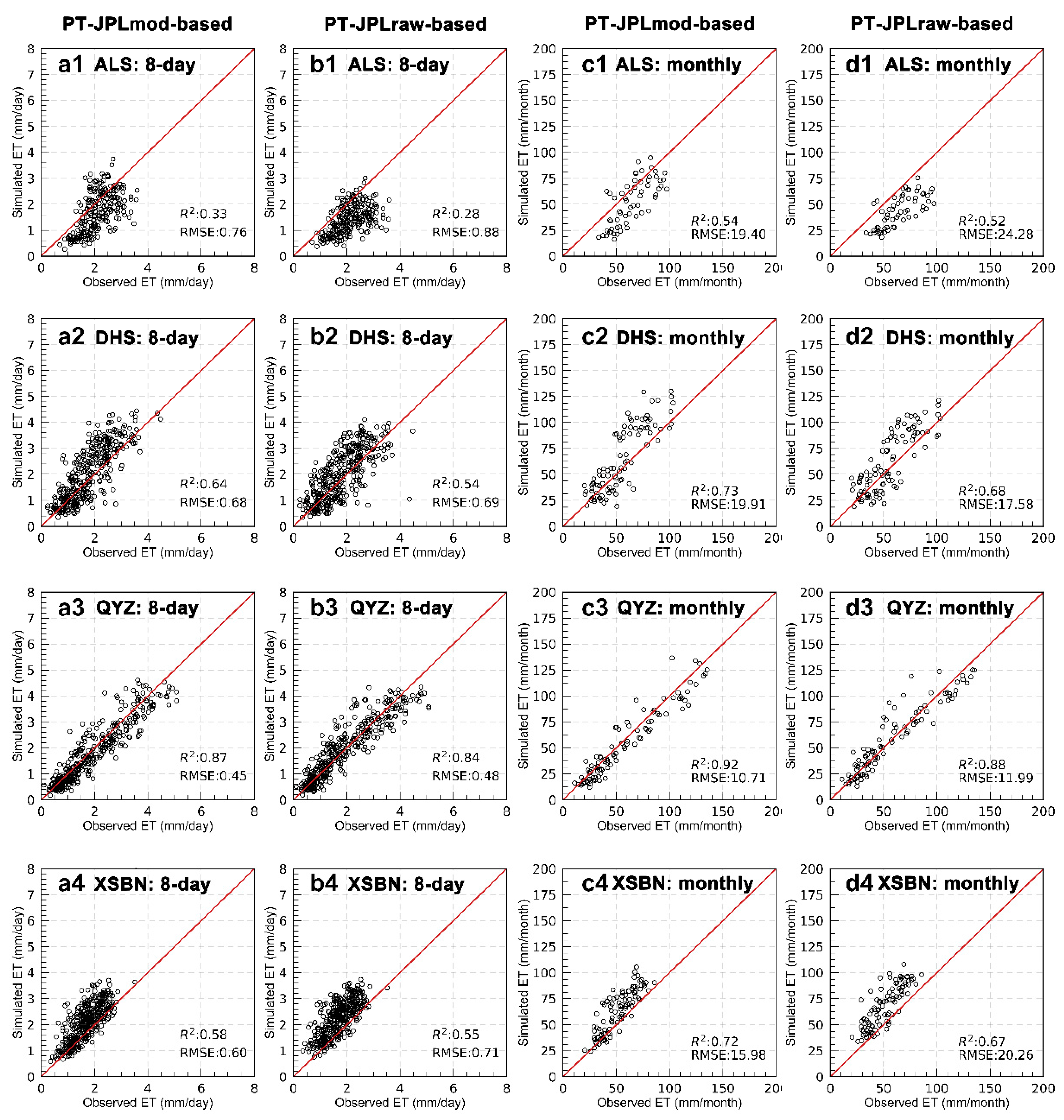
3.1. Model’s Performance

Four flux-site-derived ET data sets (i.e., monthly and 8-day average ET) (Table S2) were used to validate the modified PT-JPL (PT-JPLmod) model in our study (Figure 3 and Figure S3). The performance of the PT-JPLmod model in simulating ET was also compared with that of the original PT-JPL (PT-JPLraw) model. As seen, all the PT-JPL models showed a good performance in simulating the subtropical forest ET (Figure 3). However, compared to the PT-JPLraw model, the PT-JPLmod model improved the accuracy of the ET simulation at the 8-day scale and monthly scale (Figure 3 and Figure S3). For the 8-day scale, the mean of R2 and RMSE for the PT-JPLraw model in simulation of ET at the four flux tower sites was 0.55 and 0.69 mm day−1 (Figure 3(a1–a4) and Figure S3), respectively, while the accuracy of the ET simulations based on the improved PT-JPL model is relatively improved (R2 = 0.61 and RMSE = 0.51 mm day−1) (Figure 3(a1–a4) and Figure S3). A similar enhancement of the accuracy at the monthly scale was also observed (Figure 3(c1–c4) and Figure S3).
We incorporated the PT-JPLmod model into the raw analytical WUE model, and this was used to simulate the annual WUE of the subtropical forests. The observed WUE derived from the flux towers and the published literature (see Tables S2 and S3 and Figure 1) was utilized to validate the simulated WUE in this study. The simulated WUE based on our improved analytical WUE model was highly correlated with the observed WUE (R2 = 0.76 and RMSE = 0.41 gC kg−1 H2O) (Figure 4a). The original PT-JPL model was also coupled to the WUE model to simulate WUE and further compared with our improved WUE model on simulated WUE. The evaluation also demonstrated that the accuracy of our simulated WUE can be improved in terms of R2 and RMSE (Figure 4a,b). To further confirm the simulation accuracy of our model, we calculated the ratio of Ei to ET in the analytical WUE model based on the PML and GLEAM datasets, which were respectively used to simulate annual WUE. The simulated WUE (PML) and WUE (GLEAM) also showed relatively lower R2 (0.69 and 0.67) and higher RMSE (0.46 gC kg−1 H2O and 0.45 gC kg−1 H2O) (Figure 4c,d) than our simulated WUE (R2 = 0.76 and RMSE = 0.41 gC kg−1 H2O) (Figure 4a), suggesting that the simulated WUE can achieve a higher accuracy by using our developed WUE framework. Additionally, these results also indirectly demonstrated that the original PT-JPL model can be improved by incorporating the modified Gash model.

3.2. Spatial Pattern and Temporal Changes in Subtropical Forest WUE

The multi-year (2001–2018) mean WUE of China’s subtropical forests showed spatial heterogeneity (Figure 5a). WUE values greater than 3.0 gC kg−1 H2O were mainly located in the east, while those less than 2.5 gC kg−1 H2O were mainly found in the west (Figure 5a). Spatially, the WUE values between 2.5 and 3 gC kg−1 H2O accounted for the largest proportion (38.72%) of the total area. Different forest types also showed different WUE values in the subtropical region. The mixed forest had the highest WUE (3.65 ± 0.86 gC kg−1 H2O) (mean ± std dev.), followed by the deciduous broad-leaved forest (2.72 ± 0.57 gC kg−1 H2O), evergreen needle-leaved forest (2.63 ± 0.62 gC kg−1 H2O), and evergreen broad-leaved forest (2.61 ± 0.49 gC kg−1 H2O) (Figure 5b). The regional-averaged value of the forest WUE was 2.84 ± 0.75 gC kg−1 H2O.
From 2001 to 2018, a significant increasing trend (0.025 gC kg−1 H2O year−1; p < 0.001) in the WUE of China’s subtropical forests was found (Figure 6a). The WUE of EBF and DBF showed the largest increasing trend, with a growth rate of 0.027 gC kg−1 H2O year−1 (p < 0.001) (Figure 6b,c), compared with the trends in ENF (0.021 gC kg−1 H2O year−1; p < 0.001) and MXF (0.025 gC kg−1 H2O year−1; p < 0.001) (Figure 6d,e). Spatially, the increased WUE accounted for 87.1% (significant increase trends accounted for 63.8%) of the total area (Figure 6f), which was distributed throughout the study area from east to west. Conversely, the declined WUE (12.9%) mostly occurred in the west and northwest (Figure 6f).

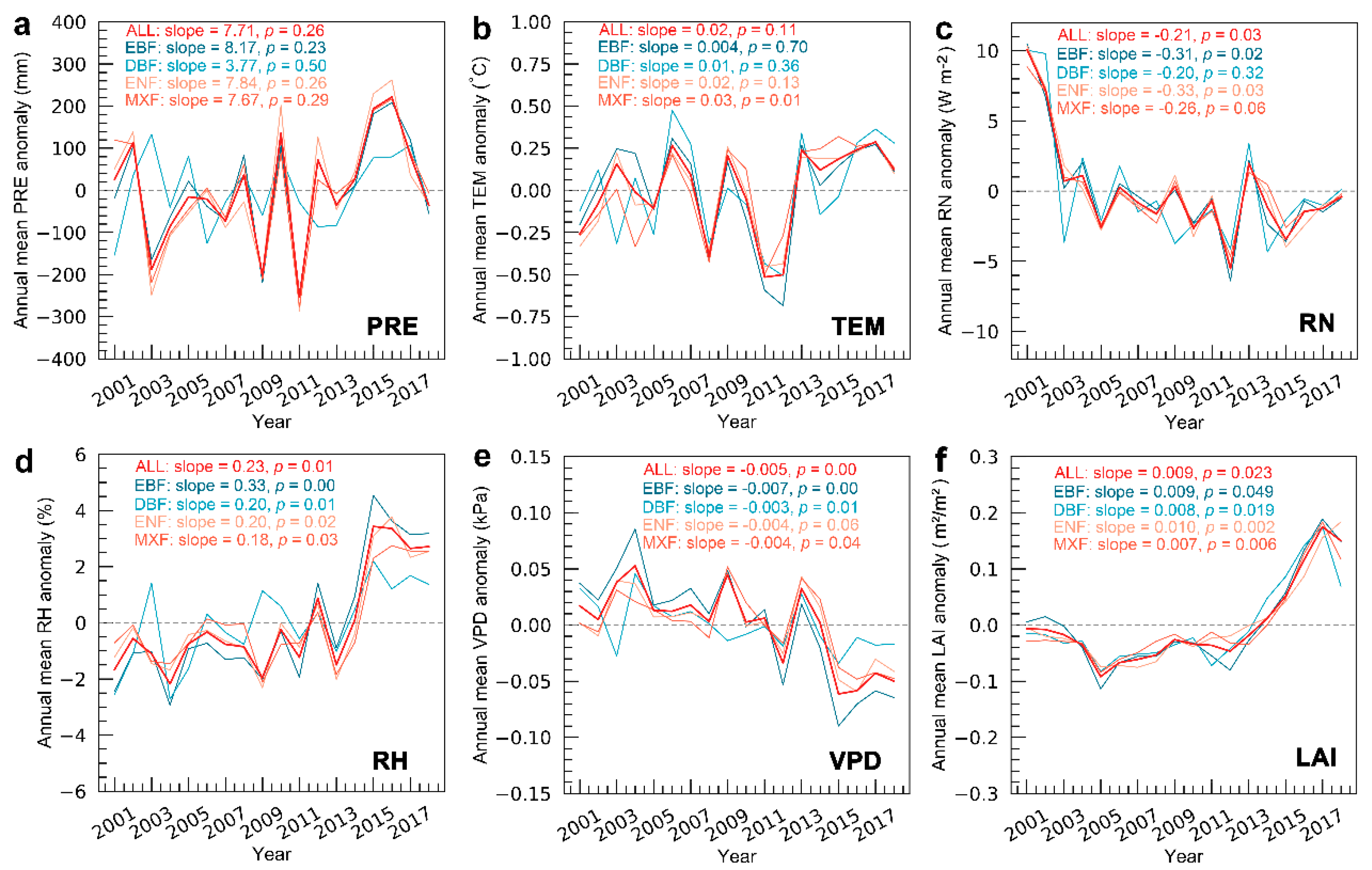
3.3. Variation Characteristics of Climate Variables, LAI, and Atmospheric CO2

The annual variation characteristics of the main climate variables (i.e., PRE, TEM, RN, RH, and VPD) were investigated during 2001–2018 (Figure 7a–e). Generally, the PRE, TEM, and RH showed gradually increasing trends in the entire forest region, with annual change rates of 7.71 mm year−1, 0.02 °C year−1, and 0.23% year−1 (Figure 7a,b,d). The same increasing trends for different forest types were also observed during 2001–2018. Especially, the RH of the entire and different forest regions significantly increased at the rate of 0.23% year−1 (p = 0.01) (ALL), 0.33% year−1 (p = 0.00) (EBF), 0.20% year−1 (p = 0.01) (DBF), 0.20% year−1 (p = 0.02) (ENF), and 0.18% year−1 (p = 0.03) (MXF), respectively (Figure 7d). However, the annual variations in RN and VPD in the entire forest region showed a significant downward trend at a rate of 0.21 W m−2 year−1 (p = 0.03) and 0.005 kPa/year (p = 0.00), respectively (Figure 7c,e).
Annual variations in the vegetation, as indicated by the LAI, presented a significant upward trend during 2001–2018, with a trend of 0.009 m2 m−2 year−1 (p = 0.023) for the entire study area (Figure 7f), as well as a trend of 0.009 m2 m−2 year−1 (p = 0.049) for EBF, 0.008 m2 m−2 year−1 (p = 0.019) for DBF, 0.010 m2 m−2 year−1 (p = 0.002) for ENF, and 0.007 m2 m−2 year−1 (p = 0.006) for MXF, respectively (Figure 7f). We also analyzed the annual changes in the atmospheric CO2 concentration from 2001 to 2018 (Figure S2). The CO2 concentration increased from 371.3 ppm in 2001 to 408.7 ppm in 2018, with a growth rate of 2.14 ppm year−1 (p = 0.00).
The annual variation in the main climatic factors and LAI presented obvious spatial heterogeneity across the study area (Figure 8). The PRE in most areas showed an increasing trend, accounting for 84.9% of the total study area. TEM also presented an upward trend in a large part of the study area (78.0%) and 36.9% of the increased area showed a significant upward trend (36.9%), while a significantly declined TEM was observed in the west (Figure 8b). In terms of the RH, the significant increasing trend accounting for 46.5% of the increasing area was found from the east to west; the trend of the RH in the same area in the west was opposite to that of TEM (Figure 8b,d). Under the combined effects of the TEM and RH, a large part (40.9%) of the VPD significantly declined during the study period, while the areas where VPD increased significantly (23.7%) were mainly scattered in the south, north, and west (Figure 8e). As for RN, it was almost on a downward trend (88.1%) during 2001–2018, especially in the eastern and southern regions, where RN showed a significant decreasing trend (38.0%) (Figure 8c). Spatially, the LAI located in the west and some portions of the east showed a decreasing trend (29.5%). The significant degradation of LAI in the western part of the study area is primarily due to a decrease in temperature in a similar region (Figure 8b). At higher altitudes, where temperatures are already relatively low, further reductions in temperature lead to a decline in vegetation vigour, thus inhibiting vegetation growth and LAI increases. In some areas of the east, the decline in LAI may be a result of urbanization, leading to the conversion from forest to non-forest and reduced solar radiation (Figure 8c). However, the LAI in the subtropical forest area mainly showed an increasing trend (70.5%), of which the significantly increased area accounted for 40.2% (Figure 8f), indicating that the vegetation in this area has recovered significantly during the past 20 years.

3.4. Contributions of Climate Variables, LAI, and Atmospheric CO2 to the Subtropical Forest WUE

3.4.1. Changes in WUE Induced by Different Drivers

The different drivers of trends in δWUE are illustrated in Figure 9 and Table 2. For the subtropical forest region, the PRE, RN, and RH mainly induced the annual δWUE to decrease. Among them, the significant decrease in WUE induced by PRE, RN, and RH accounted for 29.3%, 43.3%, and 32.7% of the total study area, respectively (Figure 9a,c,d). Conversely, the TEM, VPD, LAI, and CO2 mainly caused most portions of WUE to increase. The significant increasing trends in TEM-induced and LAI-induced δWUE were 52.1% and 27.6%. Specifically, the magnitude of δWUE induced by VPD and CO2 was higher than that of other driving factors. The obvious increasing trends in VPD-induced δWUE accounted for 29.1% of the total area, which exceeded 60 × 10−3 gC kg−1 H2O year−1 in partial regions of the west and south (Figure 9e). Trends in CO2-induced δWUE were totally positive in the study area (Figure 9g), and the values were mostly more than 10 × 10−3 gC kg−1 H2O year−1, suggesting the key role of rising CO2 concentration in inducing the growth of the forest WUE.
When considering the entire subtropical forest (i.e., ALL) and different forest types (i.e., EBF, DBF, ENF, and MXF), the trends in VPD-induced and CO2-induced δWUE are the largest (Figure 10). Moreover, the CO2-induced δWUE was larger than VPD-induced δWUE (Figure 10c–e) for DBF, ENF, and MXF, except for EBF (the VPD-induced δWUE: 19.3 × 10⁻³ gC kg−1 H2O year−1 vs. the CO2-induced δWUE: 15.9 × 10⁻³ gC kg−1 H2O year−1) (Figure 10b). Overall, for the entire study area, the CO2-induced δWUE was 16.2 × 10⁻³ gC kg−1 H2O year−1 during 2001–2018, which was close to the VPD -induced δWUE: 15.4 × 10⁻³ gC kg−1 H2O year−1 (Figure 10a), while the trends in δWUE induced by other factors were relatively minor (all within ±4 × 10⁻³ gC kg−1 H2O year−1). We summed up the trends in WUE that were induced by all drivers, and the total trend was 25.3 × 10⁻³ gC kg−1 H2O year−1, which was very close to the real trend (25.0 × 10⁻³ gC kg−1 H2O year−1) of WUE that was driven by all real driving inputs (Figure 6a).

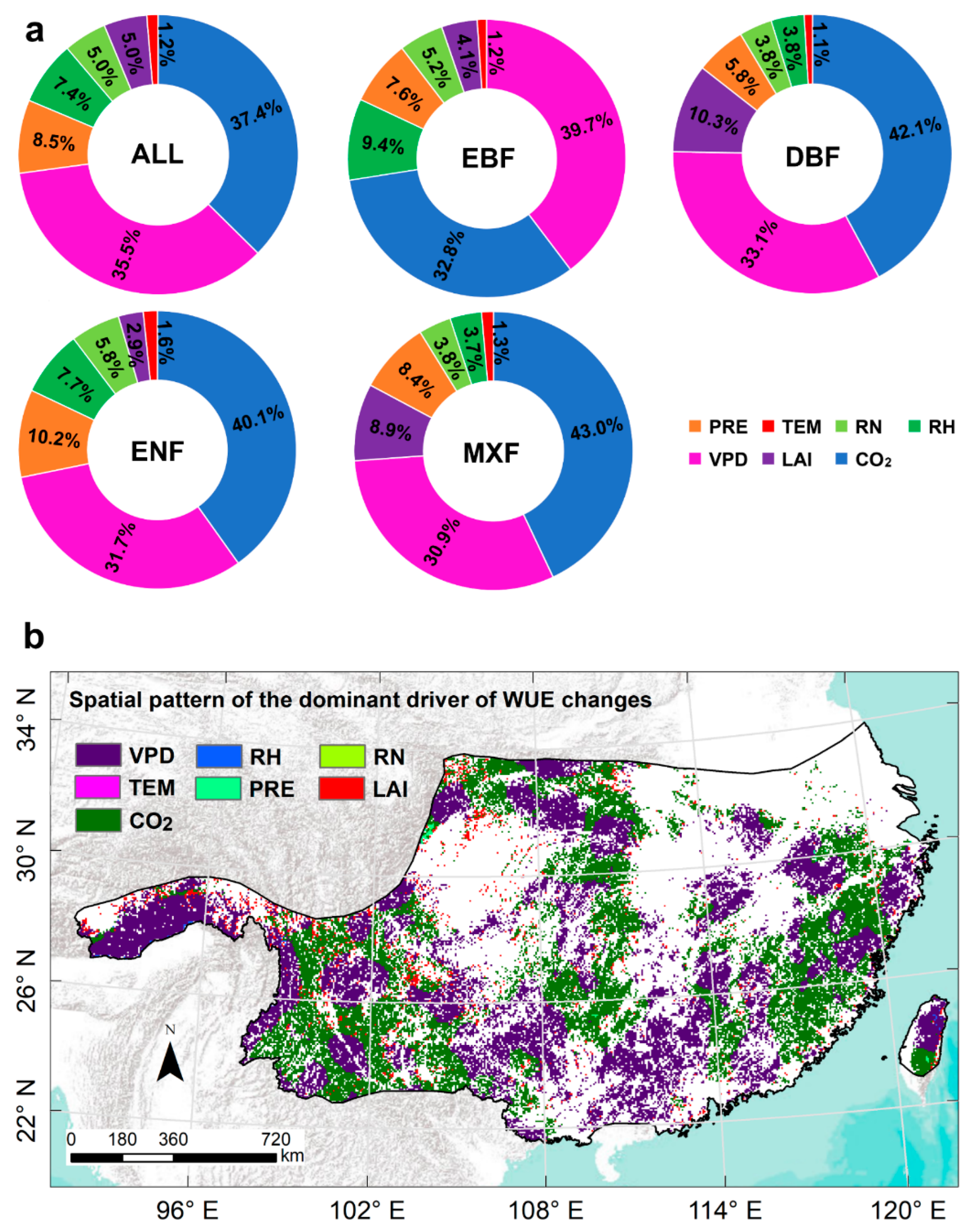
3.4.2. The Dominant Driver of the Subtropical Forest WUE Change Trends

We further calculated the relative contributions of all drivers to changes in forest WUE (Figure 11a). The CO2 was the biggest contributor to DBF, ENF, and MXF, with a β of 41.2%, 40.1%, and 43.0% (Figure 11a). However, VPD is the dominant contributor to controlling the WUE trend, with a β of 39.7% for the EBF (Figure 11a). Regarding different forests, the relative contribution of VPD was 35.5%, which was almost equal to the CO2 contribution (37.4%), indicating that the CO2 concentration and VPD were the most important and dominant drivers of WUE changes in China’s subtropical forests. For other driving factors, the contributions of PRE, RH, RN, LAI, and TEM to the annual trends of forest WUE are 8.5%, 7.4%, 5.0%, 5.0%, and 1.2%, respectively (Figure 11a).
The spatial pattern of the dominant driver of the subtropical forest WUE changes during 2001–2018 is illustrated (Figure 11b). As seen, the CO2 and VPD were staggered in the study area, with almost equal spatial impacts on WUE change trends, and individually accounted for 45.3% and 49.1% of the total study area. Additionally, LAI, as another dominant driver of WUE trends, only accounted for 5.2% of the total subtropical forested area and was mostly scattered in the northwest (Figure 11b).

4. Discussion

4.1. The Effect of Climate Change on Forest WUE Changes

The annual mean CO2 concentration increased by 37.4 ppm during 2001–2018 (Figure S2). Our study suggested that, as the largest contributor, elevated CO2 concentration has a positive impact on subtropical forest WUE (Figure 10), which also was in accordance with much of the previous research [1,6]. Using the driven- and process-based models, Huang et al. [3] reported that the rising CO2 concentration was the largest contributor to the increment of global ecosystem WUE. Some studies [75,76], based on in situ measurements (e.g., tree ring isotope), also witnessed that the forests were very sensitive to increasing CO2 concentration, especially evergreen trees. The impact mechanism of increasing CO2 concentration on WUE changes mainly includes two aspects: direct and indirect effects. Firstly, according to Equation (6) in the analytical WUE model, the CO2 concentration is positively correlated with WUE; thus, the rising CO2 concentration can directly drive an increase in WUE to some extent. As for the indirect effects, the increasing CO2 concentration will not only affect the photosynthesis of vegetation, but also control its stomatal conductance and transpiration processes [1,77,78], thereby affecting WUE. For example, an increase in CO2 concentration leads to a decrease in stomatal conductance and transpiration rate while promoting photosynthetic rate, thus increasing WUE. Some studies showed that the photosynthetic efficiency of vegetation did not increase after the increase in CO2 concentration, and the increase in WUE was caused by the decrease in stomatal conductance and transpiration [79]. Keenan et al. [1], based on flux observations, found that the significant increase in WUE in temperate and boreal forests in the Northern Hemisphere was due to plants’ efforts to maintain a constant ratio (i.e., Ci/Ca) of intercellular CO2 (Ci) to atmospheric CO2 concentration (Ca). As a result, the WUE depends only on atmospheric CO2 concentration, and an increase in CO2 concentration will directly promote the WUE increase. However, it remains unclear to what extent forest WUE is limited by CO2, and the long-term effects of CO2 fertilization on ecosystem WUE need further investigation.
In our study, we found that precipitation showed an upward trend and had a negative impact on forest WUE (Figure 10). This finding is in contrast with previous studies, which focused on water-limited areas with grassland or shrubland ecosystems, such as Central Asia [80], Northern China [8], the Loess Plateau [81], and the Tibetan Plateau [7], and suggested a positive impact of precipitation on WUE. The reason for this is that increases in precipitation in water-limited regions can replenish soil moisture and mitigate the drought stress on vegetation growth, thereby promoting the WUE [8]. However, in humid regions, vegetation growth may not be sensitive to the sufficient water supply. In contrast, more precipitation in water-rich areas could enhance the interception ratio and result in fEi increases. As a result, the increase in precipitation in our study area had a negative effect on forest WUE changes. We also found that the decline in the net radiation had a negative impact on forest WUE (Figure 7c), which may be attributed to the increase in air pollution in China over the past two decades [82]. The reduction in net radiation could cause the Et and Es to decrease, and further result in the reduction in the total ET and WUE.
VPD was regarded as a determining driver of vegetation productivity and water use [83,84]. In this study, we found that VPD, rather than the LAI, was the second largest contributor to forest WUE increase, in agreement with previous studies [85,86]. However, some studies did not observe a similar relationship, which mainly derives from the difference in temporal scales used in different studies [37]. In this study, we observed the temperature, showing an insignificant increasing trend (p > 0.05) (Figure 7b), while the relative humidity showed a significant increasing trend (p < 0.05) (Figure 7d). The increased magnitude of relative humidity offset the negative effect of increased temperature on VPD [37], leading to a significant downward trend of VPD during the study period (Figure 7e). Generally, changes in VPD can control variations in potential evapotranspiration and atmospheric water demand, thereby negatively influencing soil moisture [87]. At the season or annual scale, there also exists a strong and negative coupling between VPD and soil moisture in the forest ecosystems [88]. Moreover, previous studies indicated that the WUE has a positive correlation with soil moisture [89,90] but a negative correlation with VPD [44,84,91]. Therefore, the VPD could influence the WUE via its effect on soil moisture. In our study, we observed a significant decrease in VPD (Figure 7f), which may alleviate the soil water stress of WUE and thus improve the WUE (Figure 10). However, the mechanism of the impacts of VPD on WUE varied over different time scales (e.g., hourly, daily, monthly, seasonal) and is relatively complex; thus, future studies should consider this aspect [37,88]. Importantly, our study, at the annual scale, confirmed that the CO2 concentrations and VPD played a pivotal role in subtropical forest WUE changes (Figure 11), reminding us that more attention should be paid to the long-term impacts of climate change on future forest management.

4.2. The Effect of Vegetation Greening on Forest WUE Changes

Vegetation greening occurred in China over the past few decades and was mainly attributed to several key ecological programs’ implementation [16,19,92]. Recently, the LAI in China has significantly improved, as reported by many previous studies [17,18,93]. In our study, we also found that the LAI of different forests exhibited significant (p < 0.05) enhancement during 2001–2018 (Figure 7f). Many studies have estimated the impacts of LAI on WUE and confirmed its important role in WUE changes [6,37,94,95]. In our study, we proved that the LAI was also a positive driver of subtropical forest WUE changes (Figure 10). Nevertheless, our findings showed that the LAI was not the dominant driver of WUE changes in our study area (Figure 11), which is inconsistent with previous studies based on the original analytical WUE model [6,37]. The reason for this is that these studies only considered the positive effect of the increasing LAI on the WUE via Beer’s Law [44], thus leading to a higher WUE. However, the WUE was also influenced by ET partitioning (e.g., Ei). For example, changes in LAI can also affect the allocation of water (e.g., precipitation). The increased LAI, as in our study area with dense forest coverage, could significantly increase the interception ratio, thereby reducing the WUE [96,97]. Our study used the improved analytical WUE model, which considered the impacts of the precipitation and LAI on Ei and the negative contribution of LAI to WUE, thus offsetting the overestimation of the positive impact of LAI on WUE changes. The results were consistent with the previous study [38], which also reported that increased LAI caused increased Ei and thus weekend the positive impact of vegetation restoration on WUE in the subtropical forests. However, this aspect was generally ignored in previous studies, which may enhance the role of vegetation greening in ecosystem WUE change trends. Therefore, future ecological projects should consider a reasonable vegetation restoration strategy to overcome the negative impact of vegetation restoration on Ei and WUE.

4.3. Model and Uncertainties

The analytical WUE model offers a unique and simple way for mechanistically estimating WUE to some extent, which was adopted in the present study to simulate the WUE and to distinguish the drivers of the forest WUE change trends. We first modified the original analytical WUE model by incorporating the improved PT-JPL model. The coupled analytical WUE model (Figure 2) not only showed higher accuracy in validation by using the measured WUE (Figure 4) but also overcame the shortcomings of the original analytical WUE model that cannot be used to diagnose some other key drivers (e.g., climatic factors) of the WUE change trends [6,37,39]. Therefore, this study improved the original analytical WUE model and further provided a robust and simple framework for estimating the impacts of biotic and abiotic factors on WUE changes. However, human activities, particularly soil and water conservation measures, can influence soil moisture and vegetation site conditions, thereby significantly affecting photosynthesis, transpiration and WUE. The effect of human activities on WUE was not fully considered in this study, mainly due to the limitations of the present model structure. Therefore, soil water conditions could be coupled into our model to quantify the effect of soil moisture on WUE changes in future studies. Moreover, new methods could be developed to quantitatively evaluate the individual impacts of human activities on WUE changes, such as distinguishing between climate-change-induced LAI and human-activity-induced LAI, and using these two LAIs to drive model to quantify the individual impact of climate change or human activities on WUE changes.
However, this study still has some limitations. Due to a lack of reliable and spatially explicit CO2 concentration data, especially in China, we only used annual mean CO2 concentrations from the Mauna Loa Observatory to represent the spatial variability of CO2 concentrations in our study area and drive the WUE model. This may result in spatially overestimations or underestimations of the effect of CO2 fertilization on forest WUE, although it may be reasonable to use spatially homogeneous annual mean CO2 concentrations to estimate large-scale WUE [6,7,37]. In addition, we did not consider the possible interactions and combined effects of these driving factors [98]. For instance, the LAI can be influenced by CO2 fertilization effect and climate. Generally, the increment of CO2 concentrations can enhance the LAI; thus, the influences of CO2 concentrations and LAI on WUE may be biased in this study. The elevated CO2 concentrations can also contribute to regional climate warming, thereby influencing the VPD dynamics, and further impacting the forest WUE. Overall, further studies should adopt more accurate CO2 concentrations to represent their spatial variability and drive the model, and some new quantitative methods should be adopted to isolate the net impact of CO2 on WUE [37]. Additionally, different data sets were used to drive the model, which encountered a mismatch of different datasets in terms of their spatial resolution.

5. Conclusions

In the study, we first improved the PT-JPL model by using the modified Gash model and incorporated it into the analytical WUE model to generate a novel framework. The developed WUE framework was used to estimate the subtropical forest WUE and to distinguish the drivers of annual trends in WUE in different forests during 2001–2018. The crucial questions related to the subtropical forest WUE were addressed as follows.
(1) The entire subtropical forest WUE exhibited a significant (p < 0.001) upward trend at the rate of 0.025 gC kg−1 H2O year−1 from 2001 to 2018. The WUE of EBF and DBF showed the largest increasing trend, with a growth rate of 0.027 gC kg−1 H2O year−1 (p < 0.001). The increased and decreased forest WUE accounted for 87.1% and 12.9% of the total study area, respectively.
(2) The atmospheric CO2 concentration and VPD were the dominant drivers of annual trends in WUE across the whole and different subtropical forests, mainly due to the rising CO2 concentration and decline in VPD.
(3) For the whole subtropical forest, the relative contribution of VPD accounted for 35.5% of the total forest WUE increase, which was almost equal to the contribution of elevated CO2 (37.4%). However, the temperature in the study area contributed little to the changes in forest WUE.
(4) Spatially, the CO2 and VPD as the dominant drivers were staggered in the study area, which had an almost equal spatial impact on forest WUE changes and accounted for 45.3% and 49.1% of the total study area, respectively.
Overall, our study implied that the atmospheric CO2 concentration and VPD, rather than LAI, were the dominant drivers of annual forest WUE trends in the study area, which was inconsistent with many previous studies that emphasized the dominant role of LAI in regulating the WUE changes in China. Our findings reminded us that more attention should be paid to the long-term impact of climate change on future forest management.

Supplementary Materials

The following supporting information can be downloaded at: https://www.mdpi.com/article/10.3390/rs15092441/s1. References [45,59,99,100,101,102,103,104,105,106,107,108,109,110,111] are cited in the Supplementary Materials.

Author Contributions

Conceptualization, data curation, methodology, formal analysis, writing—original draft, writing—review and editing, T.C.; conceptualization, formal analysis, funding acquisition, project administration, writing—review and editing, G.T.; visualization, writing—review and editing, Y.Y.; data curation, methodology, writing—review and editing, Z.X.; data curation, methodology, writing—review and editing, N.J. All authors have read and agreed to the published version of the manuscript.

Funding

This work was jointly supported by the National Natural Science Foundation of China (funder: Guoping Tang; Grant No. 42171025) and the program of the China Scholarships Council (funder: Tao Chen; Grant No. 202106380124).

Data Availability Statement

All datasets used in the present study are available on request from the corresponding author.

Acknowledgments

We thank the following publicly available databases for providing all the data. The flux tower data were sourced from the ChinaFLUX network (http://www.chinaflux.org/enn/index.aspx, accessed on 31 May 2021); the GLASS LAI data was obtained from the University of Maryland (http://www.glass.umd.edu/Download.html, accessed on 15 December 2022); the CMFD was obtained from the National Tibetan Plateau Third Pole Environment Data Center (https://data.tpdc.ac.cn/en/data/8028b944-daaa-4511-8769-965612652c49, accessed on 21 December 2021); the land cover data and the CCI LC user tool were downloaded from the European Space Agency (ESA) (http://maps.elie.ucl.ac.be/CCI/viewer/, accessed on 15 January 2021); the atmospheric CO2 data was obtained from the National Oceanic and Atmospheric Administration’s Earth System Research Laboratories (https://gml.noaa.gov/aftp/data/greenhouse_gases/co2/in-situ/surface/mlo/, accessed on 22 December 2022); the GLEAM ET was provided by the Global Land Evaporation Amsterdam Model (GLEAM v3.2; https://www.gleam.eu/#downloads, accessed on 17 June 2022); the PML_V2 ET data was derived from the National Tibetan Plateau Data Center (https://data.tpdc.ac.cn/allData?searchContent=PML_V2, accessed on 18 September 2022). The MSWEP precipitation data was provided by the GloH2O (http://www.gloh2o.org/mswep/, accessed on 23 December 2022).

Conflicts of Interest

The authors declare no conflict of interest.

References

  1. Keenan, T.F.; Hollinger, D.Y.; Bohrer, G.; Dragoni, D.; Munger, J.W.; Schmid, H.P.; Richardson, A.D. Increase in forest water-use efficiency as atmospheric carbon dioxide concentrations rise. Nature 2013, 499, 324–327. [Google Scholar] [CrossRef] [PubMed]
  2. Lawa, B.E.; Falge, E.; Gu, L.; Baldocchi, D.D.; Bakwin, P.; Berbigier, P.; Davis, K.; Dolman, A.J.; Falk, M.; Fuentes, J.D.; et al. Environmental controls over carbon dioxide and water vapor exchange of terrestrial vegetation. Agric. For. Meteorol. 2002, 113, 97–120. [Google Scholar] [CrossRef]
  3. Huang, M.; Piao, S.; Sun, Y.; Ciais, P.; Cheng, L.; Mao, J.; Poulter, B.; Shi, X.; Zeng, Z.; Wang, Y. Change in terrestrial ecosystem water-use efficiency over the last three decades. Glob. Chang. Biol. 2015, 21, 2366–2378. [Google Scholar] [CrossRef] [PubMed]
  4. Sun, S.; Liu, Y.; Chen, H.; Ju, W.; Xu, C.-Y.; Liu, Y.; Zhou, B.; Zhou, Y.; Zhou, Y.; Yu, M. Causes for the increases in both evapotranspiration and water yield over vegetated mainland China during the last two decades. Agric. For. Meteorol. 2022, 324, 109118. [Google Scholar] [CrossRef]
  5. Guerrieri, R.; Belmecheri, S.; Ollinger, S.V.; Asbjornsen, H.; Jennings, K.; Xiao, J.; Stocker, B.D.; Martin, M.; Hollinger, D.Y.; Bracho-Garrillo, R.; et al. Disentangling the role of photosynthesis and stomatal conductance on rising forest water-use efficiency. Proc. Natl. Acad. Sci. USA 2019, 116, 16909–16914. [Google Scholar] [CrossRef]
  6. Cheng, L.; Zhang, L.; Wang, Y.P.; Canadell, J.G.; Chiew, F.H.S.; Beringer, J.; Li, L.; Miralles, D.G.; Piao, S.; Zhang, Y. Recent increases in terrestrial carbon uptake at little cost to the water cycle. Nat. Commun. 2017, 8, 110. [Google Scholar] [CrossRef]
  7. Ma, N.; Zhang, Y. Contrasting Trends in Water Use Efficiency of the Alpine Grassland in Tibetan Plateau. J. Geophys. Res. Atmos. 2022, 127, e2022JD036919. [Google Scholar] [CrossRef]
  8. Yang, L.; Feng, Q.; Wen, X.; Barzegar, R.; Adamowski, J.F.; Zhu, M.; Yin, Z. Contributions of climate, elevated atmospheric CO2 concentration and land surface changes to variation in water use efficiency in Northwest China. Catena 2022, 213, 106220. [Google Scholar] [CrossRef]
  9. Thornton, P.E.; Law, B.E.; Gholz, H.L.; Clark, K.L.; Falged, E.; Ellsworthe, D.S.; Goldstein, A.H.; Monsong, R.K.; Hollinger, D.; Falk, M.; et al. Modeling and measuring the effects of disturbance history and climate on carbon and water budgets in evergreen needleleaf forests. Agric. For. Meteorol. 2002, 113, 185–222. [Google Scholar] [CrossRef]
  10. Pan, Y.; Birdsey, R.A.; Fang, J.; Houghton, R.; Kauppi, P.E.; Kurz, W.A.; Phillips, O.L.; Shvidenko, A.; Lewis, S.L.; Canadell, J.G. A large and persistent carbon sink in the world’s forests. Science 2011, 333, 988–993. [Google Scholar] [CrossRef]
  11. Mathias, J.M.; Trugman, A.T. Climate change impacts plant carbon balance, increasing mean future carbon use efficiency but decreasing total forest extent at dry range edges. Ecol. Lett. 2022, 25, 498–508. [Google Scholar] [CrossRef] [PubMed]
  12. Zhao, J.; Liu, D.; Zhu, Y.; Peng, H.; Xie, H. A review of forest carbon cycle models on spatiotemporal scales. J. Clean. Prod. 2022, 339, 130692. [Google Scholar] [CrossRef]
  13. Bonan, G.B. Forests and Climate Change: Forcings, Feedbacks, and the Climate Benefits of Forests. Science 2008, 320, 1444–1449. [Google Scholar] [CrossRef] [PubMed]
  14. Fang, J.; Tang, Y.; Son, Y. Why are East Asian ecosystems important for carbon cycle research? Sci. China Life Sci. 2010, 53, 753–756. [Google Scholar] [CrossRef] [PubMed]
  15. Yu, G.; Chen, Z.; Piao, S.; Peng, C.; Ciais, P.; Wang, Q.; Li, X.; Zhu, X. High carbon dioxide uptake by subtropical forest ecosystems in the East Asian monsoon region. Proc. Natl. Acad. Sci. USA 2014, 111, 4910–4915. [Google Scholar] [CrossRef] [PubMed]
  16. Lu, F.; Hu, H.; Sun, W.; Zhu, J.; Liu, G.; Zhou, W.; Zhang, Q.; Shi, P.; Liu, X.; Wu, X. Effects of national ecological restoration projects on carbon sequestration in China from 2001 to 2010. Proc. Natl. Acad. Sci. USA 2018, 115, 4039–4044. [Google Scholar] [CrossRef] [PubMed]
  17. Chen, C.; Park, T.; Wang, X.; Piao, S.; Xu, B.; Chaturvedi, R.K.; Fuchs, R.; Brovkin, V.; Ciais, P.; Fensholt, R.; et al. China and India lead in greening of the world through land-use management. Nat. Sustain. 2019, 2, 122–129. [Google Scholar] [CrossRef] [PubMed]
  18. Chen, J.M.; Ju, W.; Ciais, P.; Viovy, N.; Lu, X. Vegetation structural change since 1981 significantly enhanced the terrestrial carbon sink. Nat. Commun. 2019, 10, 4259. [Google Scholar] [CrossRef]
  19. Tong, X.; Brandt, M.; Yue, Y.; Horion, S.; Wang, K.; Keersmaecker, W.D.; Tian, F.; Schurgers, G.; Xiao, X.; Luo, Y. Increased vegetation growth and carbon stock in China karst via ecological engineering. Nat. Sustain. 2018, 1, 44–50. [Google Scholar] [CrossRef]
  20. Fang, J.; Yu, G.; Liu, L.; Hu, S.; Chapin, F.S. Climate change, human impacts, and carbon sequestration in China. Proc. Natl. Acad. Sci. USA 2018, 115, 4015–4020. [Google Scholar] [CrossRef]
  21. Gao, T.; Wang, H.J.; Zhou, T. Changes of extreme precipitation and nonlinear influence of climate variables over monsoon region in China. Atmos. Res. 2017, 197, 379–389. [Google Scholar] [CrossRef]
  22. Dekker, S.C.; Groenendijk, M.; Booth, B.B.B.; Huntingford, C.; Cox, P.M. Spatial and temporal variations in plant water-use efficiency inferred from tree-ring, eddy covariance and atmospheric observations. Earth Syst. Dyn. 2016, 7, 525–533. [Google Scholar] [CrossRef]
  23. CMA. China Greenhouse Gas Bulletin: The State of Greenhouse Gases in the Atmosphere Based on Chinese and Global Observations before 2017. Available online: http://www.cma.gov.cn/en2014/news/News/201901/P020190122575481732415.pdf (accessed on 21 December 2021).
  24. Sun, S.; Song, Z.; Wu, X.; Wang, T.; Wu, Y.; Du, W.; Che, T.; Huang, C.; Zhang, X.; Ping, B.; et al. Spatio-temporal variations in water use efficiency and its drivers in China over the last three decades. Ecol. Indic. 2018, 94, 292–304. [Google Scholar] [CrossRef]
  25. Sun, Y.; Piao, S.; Huang, M.; Ciais, P.; Zeng, Z.; Cheng, L.; Li, X.; Zhang, X.; Mao, J.; Peng, S.; et al. Global patterns and climate drivers of water-use efficiency in terrestrial ecosystems deduced from satellite-based datasets and carbon cycle models. Glob. Ecol. Biogeogr. 2016, 25, 311–323. [Google Scholar] [CrossRef]
  26. Xue, Y.; Liang, H.; Zhang, B.; He, C. Vegetation restoration dominated the variation of water use efficiency in China. J. Hydrol. 2022, 612, 128257. [Google Scholar] [CrossRef]
  27. Li, G.; Chen, W.; Li, R.; Zhang, X.; Liu, J. Assessing the spatiotemporal dynamics of ecosystem water use efficiency across China and the response to natural and human activities. Ecol. Indic. 2021, 126, 107680. [Google Scholar] [CrossRef]
  28. Xiao, J.; Sun, G.; Chen, J.; Chen, H.; Chen, S.; Dong, G.; Gao, S.; Guo, H.; Guo, J.; Han, S.; et al. Carbon fluxes, evapotranspiration, and water use efficiency of terrestrial ecosystems in China. Agric. For. Meteorol. 2013, 182–183, 76–90. [Google Scholar] [CrossRef]
  29. Kim, D.; Baik, J.; Umair, M.; Choi, M. Water use efficiency in terrestrial ecosystem over East Asia: Effects of climate regimes and land cover types. Sci. Total Environ. 2021, 773, 145519. [Google Scholar] [CrossRef]
  30. Lan, X.; Li, Y.; Shao, R.; Chen, X.; Lin, K.; Cheng, L.; Gao, H.; Liu, Z. Vegetation controls on surface energy partitioning and water budget over China. J. Hydrol. 2021, 600, 125646. [Google Scholar] [CrossRef]
  31. Wang, M.; Ding, Z.; Wu, C.; Song, L.; Ma, M.; Yu, P.; Lu, B.; Tang, X. Divergent responses of ecosystem water-use efficiency to extreme seasonal droughts in Southwest China. Sci. Total Environ. 2021, 760, 143427. [Google Scholar] [CrossRef]
  32. Ding, Z.; Liu, Y.; Wang, L.; Chen, Y.; Yu, P.; Ma, M.; Tang, X. Effects and implications of ecological restoration projects on ecosystem water use efficiency in the karst region of Southwest China. Ecol. Eng. 2021, 170, 106356. [Google Scholar] [CrossRef]
  33. Liu, X.; Feng, X.; Fu, B. Changes in global terrestrial ecosystem water use efficiency are closely related to soil moisture. Sci. Total Environ. 2020, 698, 134165. [Google Scholar] [CrossRef] [PubMed]
  34. Xiao, B.; Bai, X.; Zhao, C.; Tan, Q.; Li, Y.; Luo, G.; Wu, L.; Chen, F.; Li, C.; Ran, C.; et al. Responses of carbon and water use efficiencies to climate and land use changes in China’s karst areas. J. Hydrol. 2023, 617, 128968. [Google Scholar] [CrossRef]
  35. Kang, F.; Li, X.; Du, H.; Mao, F.; Zhou, G.; Xu, Y.; Huang, Z.; Ji, J.; Wang, J. Spatiotemporal Evolution of the Carbon Fluxes from Bamboo Forests and their Response to Climate Change Based on a BEPS Model in China. Remote Sens. 2022, 14, 366. [Google Scholar] [CrossRef]
  36. Xie, S.; Mo, X.; Hu, S.; Liu, S. Contributions of climate change, elevated atmospheric CO2 and human activities to ET and GPP trends in the Three-North Region of China. Agric. For. Meteorol. 2020, 295, 108183. [Google Scholar] [CrossRef]
  37. Zhao, F.; Wu, Y.; Ma, S.; Lei, X.; Liao, W. Increased Water Use Efficiency in China and Its Drivers During 2000–2016. Ecosystems 2022, 25, 1476–1492. [Google Scholar] [CrossRef]
  38. Shao, R.; Shao, W.; Gu, C.; Zhang, B. Increased Interception Induced by Vegetation Restoration Counters Ecosystem Carbon and Water Exchange Efficiency in China. Earth’s Future 2022, 10, e2021EF002464. [Google Scholar] [CrossRef]
  39. Cai, W.; Ullah, S.; Yan, L.; Lin, Y. Remote Sensing of Ecosystem Water Use Efficiency: A Review of Direct and Indirect Estimation Methods. Remote Sens. 2021, 13, 2393. [Google Scholar] [CrossRef]
  40. He, H.; Ge, R.; Ren, X.; Zhang, L.; Chang, Q.; Xu, Q.; Zhou, G.; Xie, Z.; Wang, S.; Wang, H.; et al. Reference carbon cycle dataset for typical Chinese forests via colocated observations and data assimilation. Sci. Data 2021, 8, 42. [Google Scholar] [CrossRef]
  41. He, H.; Wang, S.; Zhang, L.; Wang, J.; Ren, X.; Zhou, L.; Piao, S.; Yan, H.; Ju, W.; Gu, F.; et al. Altered trends in carbon uptake in China’s terrestrial ecosystems under the enhanced summer monsoon and warming hiatus. Natl. Sci. Rev. 2019, 6, 505–514. [Google Scholar] [CrossRef]
  42. Zhang, R.; Zhou, X.; Ouyang, Z.; Avitabile, V.; Qi, J.; Chen, J.; Giannico, V. Estimating aboveground biomass in subtropical forests of China by integrating multisource remote sensing and ground data. Remote Sens. Environ. 2019, 232, 111341. [Google Scholar] [CrossRef]
  43. Wong, S.C.; Cowan, I.R.; Farquhar, G.D. Stomatal conductance correlates with photosynthetic capacity. Nature 1979, 282, 424–426. [Google Scholar] [CrossRef]
  44. Beer, C.; Ciais, P.; Reichstein, M.; Baldocchi, D.; Law, B.E.; Papale, D.; Soussana, J.F.; Ammann, C.; Buchmann, N.; Frank, D.; et al. Temporal and among-site variability of inherent water use efficiency at the ecosystem level. Glob. Biogeochem. Cycles 2009, 23, GB2018. [Google Scholar] [CrossRef]
  45. Fisher, J.B.; Tu, K.P.; Baldocchi, D.D. Global estimates of the land–atmosphere water flux based on monthly AVHRR and ISLSCP-II data, validated at 16 FLUXNET sites. Remote Sens. Environ. 2008, 112, 901–919. [Google Scholar] [CrossRef]
  46. Sawano, S.; Hotta, N.; Tanaka, N.; Tsuboyama, Y.; Suzuki, M. Development of a simple forest evapotranspiration model using a process-oriented model as a reference to parameterize data from a wide range of environmental conditions. Ecol. Model. 2015, 309–310, 93–109. [Google Scholar] [CrossRef]
  47. Miralles, D.G.; Holmes, T.R.H.; De Jeu, R.A.M.; Gash, J.H.; Meesters, A.G.C.A.; Dolman, A.J. Global land-surface evaporation estimated from satellite-based observations. Hydrol. Earth Syst. Sci. 2011, 15, 453–469. [Google Scholar] [CrossRef]
  48. Ma, N.; Zhang, Y. Increasing Tibetan Plateau terrestrial evapotranspiration primarily driven by precipitation. Agric. For. Meteorol. 2022, 317, 108887. [Google Scholar] [CrossRef]
  49. Niu, Z.; He, H.; Zhu, G.; Ren, X.; Zhang, L.; Zhang, K. A spatial-temporal continuous dataset of the transpiration to evapotranspiration ratio in China from 1981–2015. Sci. Data 2020, 7, 369. [Google Scholar] [CrossRef]
  50. Talsma, C.J.; Good, S.P.; Jimenez, C.; Martens, B.; Fisher, J.B.; Miralles, D.G.; McCabe, M.F.; Purdy, A.J. Partitioning of evapotranspiration in remote sensing-based models. Agric. For. Meteorol. 2018, 260–261, 131–143. [Google Scholar] [CrossRef]
  51. Miralles, D.G.; Jiménez, C.; Jung, M.; Michel, D.; Ershadi, A.; McCabe, M.F.; Hirschi, M.; Martens, B.; Dolman, A.J.; Fisher, J.B.; et al. The WACMOS-ET project–Part 2: Evaluation of global terrestrial evaporation data sets. Hydrol. Earth Syst. Sci. 2016, 20, 823–842. [Google Scholar] [CrossRef]
  52. Luo, Z.; Guo, M.; Bai, P.; Li, J. Different Vegetation Information Inputs Significantly Affect the Evapotranspiration Simulations of the PT-JPL Model. Remote Sens. 2022, 14, 2573. [Google Scholar] [CrossRef]
  53. van Dijk, A.I.J.M.; Bruijnzeel, L.A. Modelling rainfall interception by vegetation of variable density using an adapted analytical model. Part 1. Model description. J. Hydrol. 2001, 247, 230–238. [Google Scholar] [CrossRef]
  54. Gash, J.H.C. An analytical model of rainfall interception by forests. Q. J. R. Meteorol. Soc. 1979, 105, 43–55. [Google Scholar] [CrossRef]
  55. Zhang, Y.; Kong, D.; Gan, R.; Chiew, F.H.S.; McVicar, T.R.; Zhang, Q.; Yang, Y. Coupled estimation of 500 m and 8-day resolution global evapotranspiration and gross primary production in 2002–2017. Remote Sens. Environ. 2019, 222, 165–182. [Google Scholar] [CrossRef]
  56. Yu, G.-R.; Wen, X.-F.; Sun, X.-M.; Tanner, B.D.; Lee, X.; Chen, J.-Y. Overview of ChinaFLUX and evaluation of its eddy covariance measurement. Agric. For. Meteorol. 2006, 137, 125–137. [Google Scholar] [CrossRef]
  57. Martens, B.; Miralles, D.G.; Lievens, H.; van der Schalie, R.; de Jeu, R.A.M.; Fernández-Prieto, D.; Beck, H.E.; Dorigo, W.A.; Verhoest, N.E.C. GLEAM v3: Satellite-based land evaporation and root-zone soil moisture. Geosci. Model Dev. 2017, 10, 1903–1925. [Google Scholar] [CrossRef]
  58. Zhang, Y.; Peña-Arancibia, J.L.; McVicar, T.R.; Chiew, F.H.S.; Vaze, J.; Liu, C.; Lu, X.; Zheng, H.; Wang, Y.; Liu, Y.Y.; et al. Multi-decadal trends in global terrestrial evapotranspiration and its components. Sci. Rep. 2016, 6, 19124. [Google Scholar] [CrossRef] [PubMed]
  59. Xiao, Z.; Liang, S.; Wang, J.; Xiang, Y.; Zhao, X.; Song, J. Long-Time-Series Global Land Surface Satellite Leaf Area Index Product Derived from MODIS and AVHRR Surface Reflectance. IEEE Trans. Geosci. Remote Sens. 2016, 54, 5301–5318. [Google Scholar] [CrossRef]
  60. Xie, X.; Li, A.; Jin, H.; Tan, J.; Wang, C.; Lei, G.; Zhang, Z.; Bian, J.; Nan, X. Assessment of five satellite-derived LAI datasets for GPP estimations through ecosystem models. Sci. Total Environ. 2019, 690, 1120–1130. [Google Scholar] [CrossRef]
  61. Liu, Y.; Xiao, J.; Ju, W.; Zhu, G.; Wu, X.; Fan, W.; Li, D.; Zhou, Y. Satellite-derived LAI products exhibit large discrepancies and can lead to substantial uncertainty in simulated carbon and water fluxes. Remote Sens. Environ. 2018, 206, 174–188. [Google Scholar] [CrossRef]
  62. He, J.; Yang, K.; Tang, W.; Lu, H.; Qin, J.; Chen, Y.; Li, X. The first high-resolution meteorological forcing dataset for land process studies over China. Sci. Data 2020, 7, 25. [Google Scholar] [CrossRef]
  63. Huang, J.; Zhang, Y.; Bing, H.; Peng, J.; Dong, F.; Gao, J.; Arhonditsis, G.B. Characterizing the river water quality in China: Recent progress and on-going challenges. Water Res. 2021, 201, 117309. [Google Scholar] [CrossRef] [PubMed]
  64. Wang, B.; Ma, Y.; Su, Z.; Wang, Y.; Ma, W. Quantifying the evaporation amounts of 75 high-elevation large dimictic lakes on the Tibetan Plateau. Sci. Adv. 2020, 6, eaay8558. [Google Scholar] [CrossRef] [PubMed]
  65. Yang, F.; Lu, H.; Yang, K.; He, J.; Wang, W.; Wright, J.S.; Li, C.; Han, M.; Li, Y. Evaluation of multiple forcing data sets for precipitation and shortwave radiation over major land areas of China. Hydrol. Earth Syst. Sci. 2017, 21, 5805–5821. [Google Scholar] [CrossRef]
  66. Beck, H.E.; Wood, E.F.; Pan, M.; Fisher, C.K.; Miralles, D.G.; van Dijk, A.I.J.M.; McVicar, T.R.; Adler, R.F. MSWEP V2 Global 3-Hourly 0.1° Precipitation: Methodology and Quantitative Assessment. Bull. Am. Meteorol. Soc. 2019, 100, 473–500. [Google Scholar] [CrossRef]
  67. Wu, J.; Gao, X.-J. A gridded daily observation dataset over China region and comparison with the other datasets. Chin. J. Geophys. 2013, 56, 1102–1111. [Google Scholar]
  68. Buck, A.L. New Equations for Computing Vapor Pressure and Enhancement Factor. J. Appl. Meteorol. Climatol. 1981, 20, 1527–1532. [Google Scholar] [CrossRef]
  69. Jiang, B.; Liang, S.; Jia, A.; Xu, J.; Zhang, X.; Xiao, Z.; Zhao, X.; Jia, K.; Yao, Y. Validation of the Surface Daytime Net Radiation Product from Version 4.0 GLASS Product Suite. IEEE Geosci. Remote Sens. Lett. 2019, 16, 509–513. [Google Scholar] [CrossRef]
  70. ESA. Land Cover CCI: Product User Guide Version 2.0. 2017. Available online: https://maps.elie.ucl.ac.be/CCI/viewer/download/ESACCI-LC-Ph2-PUGv2_2.0.pdf (accessed on 15 January 2022).
  71. Tagesson, T.; Schurgers, G.; Horion, S.; Ciais, P.; Tian, F.; Brandt, M.; Ahlstrom, A.; Wigneron, J.P.; Ardo, J.; Olin, S.; et al. Recent divergence in the contributions of tropical and boreal forests to the terrestrial carbon sink. Nat. Ecol. Evol. 2020, 4, 202–209. [Google Scholar] [CrossRef]
  72. Peng, J.; Wu, C.; Zhang, X.; Ju, W.; Wang, X.; Lu, L.; Liu, Y. Incorporating water availability into autumn phenological model improved China’s terrestrial gross primary productivity (GPP) simulation. Environ. Res. Lett. 2021, 16, 094012. [Google Scholar] [CrossRef]
  73. Wang, X.; Chen, J.M.; Ju, W.; Zhang, Y. Seasonal Variations in Leaf Maximum Photosynthetic Capacity and Its Dependence on Climate Factors Across Global FLUXNET Sites. J. Geophys. Res. Biogeosci. 2022, 127, e2021JG006709. [Google Scholar] [CrossRef]
  74. Sen, P.K. Estimates of the Regression Coefficient Based on Kendall’s Tau. J. Am. Stat. Assoc. 1968, 63, 1379–1389. [Google Scholar] [CrossRef]
  75. Battipaglia, G.; Saurer, M.; Cherubini, P.; Calfapietra, C.; McCarthy, H.R.; Norby, R.J.; Francesca Cotrufo, M. Elevated CO2 increases tree-level intrinsic water use efficiency: Insights from carbon and oxygen isotope analyses in tree rings across three forest FACE sites. New Phytol. 2013, 197, 544–554. [Google Scholar] [CrossRef] [PubMed]
  76. Soh, W.K.; Yiotis, C.; Murray, M.; Parnell, A.; Wright, I.J.; Spicer, R.A.; Lawson, T.; Caballero, R.; McElwain, J.C. Rising CO2 drives divergence in water use efficiency of evergreen and deciduous plants. Sci. Adv. 2019, 5, eaax7906. [Google Scholar] [CrossRef]
  77. Chen, C.; Riley, W.J.; Prentice, I.C.; Keenan, T.F. CO2 fertilization of terrestrial photosynthesis inferred from site to global scales. Proc. Natl. Acad. Sci. USA 2022, 119, e2115627119. [Google Scholar] [CrossRef] [PubMed]
  78. Gentine, P.; Green, J.K.; Guérin, M.; Humphrey, V.; Seneviratne, S.I.; Zhang, Y.; Zhou, S. Coupling between the terrestrial carbon and water cycles—A review. Environ. Res. Lett. 2019, 14, 083003. [Google Scholar] [CrossRef]
  79. Rogers, H.H.; Runion, G.B.; Krupa, S.V. Plant responses to atmospheric CO2 enrichment with emphasis on roots and the rhizosphere. Environ. Pollut. 1994, 83, 155–189. [Google Scholar] [CrossRef]
  80. Zhang, L.; Xiao, J.; Zheng, Y.; Li, S.; Zhou, Y. Increased carbon uptake and water use efficiency in global semi-arid ecosystems. Environ. Res. Lett. 2020, 15, 034022. [Google Scholar] [CrossRef]
  81. Zhang, T.; Peng, J.; Liang, W.; Yang, Y.; Liu, Y. Spatial-temporal patterns of water use efficiency and climate controls in China’s Loess Plateau during 2000–2010. Sci. Total Environ. 2016, 565, 105–122. [Google Scholar] [CrossRef]
  82. Zhang, Y.; Song, C.; Zhang, K.; Cheng, X.; Band, L.E.; Zhang, Q. Effects of land use/land cover and climate changes on terrestrial net primary productivity in the Yangtze River Basin, China, from 2001 to 2010. J. Geophys. Res. Biogeosci. 2014, 119, 1092–1109. [Google Scholar] [CrossRef]
  83. Yuan, W.; Zheng, Y.; Piao, S.; Ciais, P.; Lombardozzi, D.; Wang, Y.; Ryu, Y.; Chen, G.; Dong, W.; Hu, Z.; et al. Increased atmospheric vapor pressure deficit reduces global vegetation growth. Sci. Adv. 2019, 5, eaax1396. [Google Scholar] [CrossRef]
  84. Zhou, S.; Yu, B.; Huang, Y.; Wang, G. The effect of vapor pressure deficit on water use efficiency at the subdaily time scale. Geophys. Res. Lett. 2014, 41, 5005–5013. [Google Scholar] [CrossRef]
  85. Jiang, S.; Liang, C.; Cui, N.; Zhao, L.; Liu, C.; Feng, Y.; Hu, X.; Gong, D.; Zou, Q. Water use efficiency and its drivers in four typical agroecosystems based on flux tower measurements. Agric. For. Meteorol. 2020, 295, 108200. [Google Scholar] [CrossRef]
  86. Ponton, S.; Flanagan, L.B.; Alstad, K.P.; Johnson, B.G.; Morgenstern, K.A.I.; Kljun, N.; Black, T.A.; Barr, A.G. Comparison of ecosystem water-use efficiency among Douglas-fir forest, aspen forest and grassland using eddy covariance and carbon isotope techniques. Glob. Chang. Biol. 2006, 12, 294–310. [Google Scholar] [CrossRef]
  87. Berg, A.; Sheffield, J. Climate Change and Drought: The Soil Moisture Perspective. Curr. Clim. Chang. Rep. 2018, 4, 180–191. [Google Scholar] [CrossRef]
  88. Nie, C.; Huang, Y.; Zhang, S.; Yang, Y.; Zhou, S.; Lin, C.; Wang, G. Effects of soil water content on forest ecosystem water use efficiency through changes in transpiration/evapotranspiration ratio. Agric. For. Meteorol. 2021, 308–309, 108605. [Google Scholar] [CrossRef]
  89. Zheng, H.; Lin, H.; Zhu, X.-J.; Jin, Z.; Bao, H. Divergent spatial responses of plant and ecosystem water-use efficiency to climate and vegetation gradients in the Chinese Loess Plateau. Glob. Planet. Chang. 2019, 181, 102995. [Google Scholar] [CrossRef]
  90. Reichstein, M.; Tenhunen, J.D.; Roupsard, O.; Ourcival, J.-m.; Rambal, S.; Miglietta, F.; Peressotti, A.; Pecchiari, M.; Tirone, G.; Valentini, R. Severe drought effects on ecosystem CO2 and H2O fluxes at three Mediterranean evergreen sites: Revision of current hypotheses? Glob. Chang. Biol. 2002, 8, 999–1017. [Google Scholar] [CrossRef]
  91. Grossiord, C.; Buckley, T.N.; Cernusak, L.A.; Novick, K.A.; Poulter, B.; Siegwolf, R.T.W.; Sperry, J.S.; McDowell, N.G. Plant responses to rising vapor pressure deficit. New Phytol. 2020, 226, 1550–1566. [Google Scholar] [CrossRef]
  92. Yu, D.Y.; Shi, P.J.; Han, G.Y.; Zhu, W.Q.; Du, S.Q.; Xun, B. Forest ecosystem restoration due to a national conservation plan in China. Ecol. Eng. 2011, 37, 1387–1397. [Google Scholar] [CrossRef]
  93. Chen, Y.; Chen, L.; Cheng, Y.; Ju, W.; Chen, H.Y.H.; Ruan, H. Afforestation promotes the enhancement of forest LAI and NPP in China. For. Ecol. Manag. 2020, 462, 117990. [Google Scholar] [CrossRef]
  94. Li, H.; Wei, M.; Dong, L.; Hu, W.; Xiong, J.; Sun, Y.; Sun, Y.; Yao, S.; Gong, H.; Zhang, Y.; et al. Leaf and ecosystem water use efficiencies differ in their global-scale patterns and drivers. Agric. For. Meteorol. 2022, 319, 108919. [Google Scholar] [CrossRef]
  95. Nandy, S.; Saranya, M.; Srinet, R. Spatio-temporal variability of water use efficiency and its drivers in major forest formations in India. Remote Sens. Environ. 2022, 269, 112791. [Google Scholar] [CrossRef]
  96. Joggi, D.; Hofer, U.; Nosberger, J. Leaf area index, canopy structure and photosynthesis of red clover (Trifolium pratense L.). Plant Cell Environ. 1983, 6, 611–616. [Google Scholar] [CrossRef]
  97. Wang, L.; Good, S.P.; Caylor, K.K. Global synthesis of vegetation control on evapotranspiration partitioning. Geophys. Res. Lett. 2014, 41, 6753–6757. [Google Scholar] [CrossRef]
  98. Razavi, S.; Gupta, H.V. What do we mean by sensitivity analysis? The need for comprehensive characterization of “global” sensitivity in Earth and Environmental systems models. Water Resour. Res. 2015, 51, 3070–3092. [Google Scholar] [CrossRef]
  99. Potter, C.S.; Randerson, J.T.; Field, C.B.; Matson, P.A.; Vitousek, P.M.; Mooney, H.A.; Klooster, S.A. Terrestrial Ecosystem Production—A Process Model-Based on Global Satellite and Surface Data. Glob. Biogeochem. Cycles 1993, 7, 811–841. [Google Scholar] [CrossRef]
  100. Impens, I.; Lemur, R. Extinction of net radiation in different crop canopies. Theor. Appl. Climatol. 1969, 17, 403–412. [Google Scholar] [CrossRef]
  101. June, T.; Evans, J.R.; Farquhar, G.D. A simple new equation for the reversible temperature dependence of photosynthetic electron transport: A study on soybean leaf. Funct. Plant Biol. 2004, 31, 275–283. [Google Scholar] [CrossRef]
  102. Ruimy, A.; Kergoat, L.; Bondeau, A. The Participants of The Potsdam NPP Model Intercomparison. Comparing global models of terrestrial net primary productivity (NPP): Analysis of differences in light absorption and light-use efficiency. Glob. Chang. Biol. 1999, 5, 56–64. [Google Scholar] [CrossRef]
  103. Niu, Z.; He, H.; Zhu, G.; Ren, X.; Zhang, L.; Zhang, K.; Zhu, X. An increasing trend in the ratio of transpiration to total terrestrial evapotranspiration in China from 1982 to 2015 caused by greening and warming. Agric. For. Meteorol. 2019, 279, 107701. [Google Scholar] [CrossRef]
  104. Hipps, L.E. Assessing the interception of photosynthetically active radiation in winter wheat. Agric. Meteorol. 1983, 28, 253–259. [Google Scholar] [CrossRef]
  105. Qi, D.; Fei, X.; Song, Q.; Zhang, Y.; Sha, L.; Liu, Y.; Zhou, W.; Lu, Z.; Fan, Z. A dataset of carbon and water fluxes observation in subtropical evergreen broad-leaved forest in Ailao Shan from 2009 to 2013. China Scientific Data, 6 March 2021. [Google Scholar] [CrossRef]
  106. Wei, Y.; Gao, S.; Zhang, X.; Geng, S.; Zhao, X.; Jiang, Z.; Wang, Y. Source area in-FLUX measurements by FSAM model over the Populus deltoides plantation in Yueyang. Sci. Silvae Sin. 2012, 48, 16–21. [Google Scholar]
  107. Wang, S.; Zhang, Q.; Yue, P.; Wang, J.; Yang, J.; Wang, W.; Ren, X. Characteristics of latent heat flux over Cunninghamia lanceolata plantations in Huitong county. J. Cent. South Univer. For. Technol. 2011, 31, 192–197. [Google Scholar]
  108. Zhao, Z. A Study on Carbon Flux between Chinese Fir Planations and Atmosphere in Subtropical Belts. Ph.D. Thesis, Central South University of Forestry and Technology, Changsha, China, 2011. [Google Scholar]
  109. Chen, Y.; Jiang, H.; Zhou, G.; Shuang, Y.; Chen, J. Estimation of CO2 fluxes and its seasonal variations from the effective management Lei bamboo (Phyllostachys Violascens). Acta Ecol. Sin. 2013, 33, 3434–3444. [Google Scholar] [CrossRef]
  110. Lin, E.; Jiang, H.; Chen, Y. Water vapor flux variation and net radiation for a Phyllostachys violascens stand in Taihuyuan. J. Zhejiang AF Univ. 2013, 30, 313–318. [Google Scholar]
  111. Zhu, X.J.; Yu, G.R.; Wang, Q.F.; Hu, Z.M.; Zheng, H.; Li, S.G.; Hao, Y.B. Spatial variability of water use efficiency in China’s terrestrial ecosystems. Glob. Planet. Chang. 2015, 129, 37–44. [Google Scholar] [CrossRef]
Figure 1. The map shows the location of the study area and the distribution of the flux towers in China’s subtropical forests. The black dots represent that only WUE data are available, while the gray dots provide both ET and WUE data.
Remotesensing 15 02441 g001
Figure 2. The framework of the hybrid analytical WUE model. The detailed description of the Et, Es, and Ei in the flowchart can be found in sections of the method.
Remotesensing 15 02441 g002
Figure 3. Comparison of simulated and observed ET at the four flux tower stations. (a1a4,b1b4) The first two columns compare the simulated ET with the measured ET at the 8-day scale. (c1c4,d1d4) The last two columns compare the simulated ET with the measured ET at a monthly scale. The results in the first (a1a4) and third columns (c1c4) were derived from our PT-JPLmod model, and the results in the second (b1b4) and fourth (d1d4) columns were derived from the PT-JPLraw model. The red line is the 1:1 line.
Remotesensing 15 02441 g003
Figure 4. Validation of annual simulated WUE using observed WUE (n = 32). (a) The simulated WUE was driven by the fEi (i.e., Ei/ET) output from our PT-JPLmod model; (b) The simulated WUE was driven by the fEi output from the PT-JPLraw model; (c) The simulated WUE was driven by the PML products (i.e., Ei/ET); (d) The simulated WUE was driven by the GLEAM products (i.e., Ei/ET). Note that all other parameters and inputs are the same when driving the WUE model.
Remotesensing 15 02441 g004
Figure 5. (a) Spatial pattern of the mean annual (2001–2018) WUE of forests in the China’s subtropical region; (b) Boxplots show the statistical results of the multi-year mean WUE for different forests. The horizontal bar graph shows the proportion of WUE at different levels.
Remotesensing 15 02441 g005
Figure 6. (ae) The interannual variation of WUE in different forests. (f) Spatial distribution of the WUE trends in the subtropical region of China; the insert in figure f denotes the WUE trends are statistically significant with p-value < 0.05.
Remotesensing 15 02441 g006
Figure 7. Temporal variations in the precipitation (PRE) (a), temperature (TEM) (b), net radiation (RN) (c), relative humidity (RH) (d), vapor pressure deficit (VPD) (e), and LAI (f) of the entire area and different forests. The bold red lines denote the average of all forests.
Remotesensing 15 02441 g007
Figure 8. Spatial distribution of trends in precipitation (a), temperature (b), net radiation (c), relative humidity (d), vapor pressure deficit (e), and LAI (f) of the subtropical forests. The black dots in the figure represent pixels with significant changes (p < 0.05).
Remotesensing 15 02441 g008
Figure 9. The spatial distributions of the trends in δWUE caused by (a) PRE, (b) TEM, (c) RN, (d) RH, (e) VPD, (f) LAI, and (g) CO2. The black dots in the figure represent pixels with significant changes (p < 0.05).
Remotesensing 15 02441 g009
Figure 10. Statistical results of the trends in δWUE caused by PRE, TEM, RN, RH, VPD, LAI, and CO2 for (a) the entire forest region (i.e., ALL) and (be) different forest types (i.e., EBF, DBF, ENF, and MXF). The grey bar (i.e., Total) denotes the sum of trends driven by all factors.
Remotesensing 15 02441 g010
Figure 11. (a) The relative contribution of each driving force to trend in annual WUE of the entire and different forests during 2001–2018. (b) Spatial pattern of the dominant driver that caused changes in annual WUE during 2001–2018.
Remotesensing 15 02441 g011
Table 1. Design of the factorial experiments for model simulations. The ○ denotes that the inputs change during 2001–2018; the ● denotes the inputs fixed at the 2001 level.
ExperimentsDrivers
PRETEMRHRNVPDLAICO2
Baseline
S1
S2
S3
S4
S5
S6
S7
Table 2. The statistics show the proportion of different drivers that lead to an increase or decrease in δWUE in the study area.
TrendsIncreaseDecrease
p < 0.05p > 0.05p < 0.05p > 0.05
PRE-induced δWUE0.7%9.2%29.3%60.8%
TEM-induced δWUE52.1%32.8%4.9%10.2%
RN-induced δWUE0.4%5.5%43.3%50.8%
RH-induced δWUE7.7%18.1%32.7%41.5%
VPD-induced δWUE29.1%41.2%7.3%22.4%
LAI-induced δWUE27.6%43.3%5.6%23.5%
CO2-induced δWUE98.8%0.2%0.0%0.0%
Disclaimer/Publisher’s Note: The statements, opinions and data contained in all publications are solely those of the individual author(s) and contributor(s) and not of MDPI and/or the editor(s). MDPI and/or the editor(s) disclaim responsibility for any injury to people or property resulting from any ideas, methods, instructions or products referred to in the content.

