Chlorophyll-Specific Absorption Coefficient of Phytoplankton in World Oceans: Seasonal and Regional Variability

Abstract

This study investigates the seasonal and regional variability in the chlorophyll-specific absorption coefficient of phytoplankton at 443 nm ($a_{\mathit{ph}}^{*}(443)$; unit: m² mg⁻¹) in surface oceans. It is focused on the time series data derived from the satellite products of chlorophyll-a (Chl-a) concentration and the phytoplankton absorption coefficient. Global estimates of $a_{\mathit{ph}}^{*}(443)$ reveal a decreasing gradient from the open ocean toward the coastal environment, with considerable spatial variance. Seasonal variations are prominent over most oceans, resulting in substantial deviations from the climatological means. A sinusoidal model was fitted to the monthly time series data to characterize the annual and semiannual features. The amplitudes and the phases of the monthly data were latitudinally dependent. The occurrence times of the maximum $a_{\mathit{ph}}^{*}(443)$ values were six months out of phase between the northern and southern hemispheres. Satellite observations present a global mean relationship between $a_{\mathit{ph}}^{*}(443)$ and Chl-a comparable with those obtained via in situ measurements. However, the seasonal/regional $a_{\mathit{ph}}^{*}(443)$ and Chl-a relationships can significantly depart from the global mean relationship. We propose a hypothesis that $a_{\mathit{ph}}^{*}(443)$ can be predicted as a function of geolocation and time. Preliminary validations with in situ matchup data confirm that the proposed model is a promising alternative to the traditional approaches requiring Chl-a as the input. The present exploration helps understand the phytoplankton biogeography and facilitates future efforts to improve bio-optical modeling, including estimating the primary production.

1. Introduction

Natural phytoplankton in surface oceans absorb sunlight for photosynthesis and are essential in determining carbon fixation and export [1,2]. Light absorption occurs in the reaction centers containing various photosynthetic pigments. The spectral absorption coefficient of phytoplankton ($a_{\mathit{ph}}(\lambda )$; unit: m⁻¹) varies with the pigment concentration and experiences inter- and intra-species variability due to the pigment packaging effect. Phytoplankton pigment composition and size structure add another source of variability to the spectral absorption coefficient [3]. Understanding phytoplankton absorption, including spectral, temporal, and spatial variability and environmental influences, is essential to solving problems of phytoplankton ecology and primary production in the world ocean [4,5].

The chlorophyll-specific absorption coefficient of phytoplankton (unit: m² mg⁻¹) links the optics and the biology of phytoplankton. Researchers usually describe $a_{\mathit{ph}}^{*}(\lambda )$ as a simplistic nonlinear function of chlorophyll-a (Chl-a) concentration (unit: mg m⁻³) [6,7,8,9], as the latter is frequently amendable in field measurements and satellite observations. Built on the idealized $a_{\mathit{ph}}^{*}(\lambda )$-Chl-a relationship, one can determine Chl-a from $a_{\mathit{ph}}^{*}(\lambda )$ inverted from satellite ocean color spectra or vice versa [10,11,12,13]. In addition, the specific phytoplankton absorption coefficient is an important component of the bio-optical models for the estimation of the primary production, especially when Chl-a is the principal input [14,15]. Another important line of the application resides in constructing the light absorption coefficient from known pigment composition. The spectral absorption coefficients of primary pigments, including chlorophyll-a, chlorophyll-b, chlorophyll-c, photosynthetically active carotenoids, and photoprotective carotenoids, have to be predetermined [16,17]. Inversely, with known $a_{\mathit{ph}}^{*}(\lambda )$, it is feasible to infer various pigment concentrations from $a_{\mathit{ph}}(\lambda )$ via spectral decomposition [3,18]. As a phytoplankton cellular property, the size-specific $a_{\mathit{ph}}^{*}(\lambda )$ spectra are critical for the retrieval of phytoplankton size classes from ocean color observations [19,20,21,22,23,24]. As an example, Uitz et al. [24] calculated the $a_{\mathit{ph}}^{*}(\lambda )$ of microphytoplankton, nanophytoplankton, and picophytoplankton using high-performance liquid chromatography (HPLC) analysis. Brewin et al. [23] inferred class-dependent specific absorption of phytoplankton from the NASA bio-Optical Marine Algorithm Dataset (NOMAD) using a three-population model. These previous efforts achieved great success in their respective domains of application.

The examination of field measurements has lent insights into the variability in the chlorophyll-specific absorption coefficient of phytoplankton in the surface ocean. Considerable evidence has shown that this specific absorption varies regionally and seasonally in response to changes in phytoplankton species, light, and nutrient conditions [9,17,25,26,27,28,29,30,31]. In coastal oceans, for example, seasonal variability in the chlorophyll-specific absorption coefficient of phytoplankton was identified in the Arctic water [28], the Black Sea [26], and the Scotian Shelf [25]. The relationship between absorption and Chl-a reportedly differed significantly concerning seasons and/or regions [9,25,26,27]. In open oceans, the specific absorption also displayed seasonal cycles significantly different from the means [17,30]. Nevertheless, understandably, the existing in situ observations are often sporadic, and the results are restricted to local regions and do not represent all seasons. Synthesizing the field measurements remains difficult, leading to limited information that can be used to model this coefficient’s seasonal variation on a global scale.

The need for the accurate estimation of primary production and ocean color inversion demands a thorough understanding of the seasonal and regional variability in $a_{\mathit{ph}}^{*}(\lambda )$ and the underlying environmental, biological, and optical mechanisms controlling $a_{\mathit{ph}}^{*}(\lambda )$. Satellite observations from the Visible Infrared Imaging Radiometer Suite (VIIRS) on board the Suomi National Polar-orbiting Partnership (SNPP) have generated global $a_{\mathit{ph}}(\lambda )$ and Chl-a data products, which can be used to compute $a_{\mathit{ph}}^{*}(\lambda )$. Such satellite observations offer us a unique opportunity to characterize the temporal and spatial variability in this bio-optical property. Henceforth, in this study, we aim to obtain a global perspective of the variability in the chlorophyll-specific absorption coefficient of phytoplankton at a blue band of 443 nm, $a_{\mathit{ph}}^{*}(443),$ with a focus on its spatial distribution and seasonal variability. A secondary objective is to assess our ability to predict $a_{\mathit{ph}}^{*}(443)$ based on the diagnostic spatial and temporal features identified herein. Aware of uncertainties with satellite ocean color observations, we note that it is not our primary task to answer the uncertainty problems associated with $a_{\mathit{ph}}^{*}(\lambda )$ estimation. In the following, we briefly describe data and methods. We then lay out the primary findings and discuss the association between the specific absorption and Chl-a concentration. Furthermore, we discuss the perspectives and problems with the newly developed method and parameterization for the prediction of Chl-a concentration.

2. Materials and Methods

2.1. Domain of Study

The analyses were conducted based on the ocean color observations of VIIRS onboard SNPP. We selected four-year-long datasets between January 2014 and December 2017 for simplicity. The primary data were Level-3 mapped daily $a_{\mathit{ph}}(\lambda )$ and Chl-a products. As the spatial resolution of satellite images (9 km) was too coarse for most inland aquatic environments, we put our emphasis on open and coastal oceans in the following context. We defined coastal oceans as those within 200 km of coastlines or shallower than 1000 m in depth while referring to the remaining vast open regions as the open ocean. A geographical illustration of open and coastal oceans is given in Figure 1.

2.2. Satellite Ocean Color Data

The VIIRS ocean color data were processed using the NOAA Multi-Sensor Level-1 to Level-2 (MSL12) ocean color data processing system [32,33]. MSL12 followed Gordon and Wang [34] and Wang [35] in performing the atmospheric correction for satellite ocean color retrievals [36]. To determine the aerosol contribution, it estimated the aerosol types with an assumption of the null contribution at the near-infrared (NIR) bands [37] for the majority of natural waters. Whenever the black pixel assumption at the NIR bands failed in turbid coastal/inland environments [38], MSL12 switched to a combination of a NIR band and a shortwave infrared (SWIR) band [35,39]. The resulting ocean color spectra, normalized water-leaving radiance (nL_w(λ)) and remote sensing reflectance (R_rs(λ)), have 6 visible bands (410, 443, 486, 551, 638, and 671 nm) and 2 NIR bands (745 and 862 nm). Validations of nL_w(λ) or R_rs(λ) have been conducted in previous works [40,41,42,43,44,45,46,47].

Chl-a concentration data were derived using the ocean color index (OCI) algorithm [48]. The algorithm divided the global waters into two components dependent on an empirical threshold value. Specifically, when R_rs(443)/R_rs(551) ≤ 2, a 4th-order polynomial function was developed and employed for the retrieval of Chl-a:

$${\log }_{10}{\left[\mathrm{Chl-a}\right]}_{\mathrm{oc}3\mathrm{v}}={\alpha }_0+{\alpha }_1{R}_m+{\alpha }_2{R_m}^2+{\alpha }_3{R_m}^3+{\alpha }_4{R_m}^4,$$

(1)

where R_m = max(log₁₀R₁, log₁₀R₂), with R₁ = R_rs(443)/R_rs(551) and R₂ = R_rs(486)/R_rs(551), and the coefficients from ${\alpha }_0$ to ${\alpha }_4$ were specifically tuned for the VIIRS sensor (hence, the OC3V algorithm). When R_rs(443)/R_rs(551) > 4, the color index (CI) scheme [49] was used,

$${\log }_{10}{\left[\mathrm{Chl-a}\right]}_{\mathrm{CI}}=216.76 \times \mathrm{CI}-0.4093,$$

(2)

where CI = R_rs(551) − 0.526 × R_rs(443) − 0.474 × R_rs(671). For 2 < R_rs(443)/R_rs(551) ≤ 4, Equations (1) and (2) were combined via a linear weighting function, Chl-a = w × [Chl-a]_oc3v + (1 − w) × [Chl-a]_CI, with w = 0.5 × (R_rs(443)/R_rs(551) − 2), to ensure the smooth transition of the retrieved Chl-a across these 2 thresholds.

The water inherent optical properties (IOPs) were derived using the approach of Shi and Wang [50]. This method is a modification of the quasi-analytical algorithm (QAA) [51] and includes R_rs(λ) at both the visible and NIR bands in the formulation to improve the estimated IOPs. Briefly, it starts with a fundamental relationship between R_rs(λ) and IOPs,

$$R_{\mathit{rs}}(\lambda )=g_1[\frac{b_b(\lambda )}{a(\lambda )+b_b(\lambda )}]+g_2{\left[\frac{b_b(\lambda )}{a(\lambda )+b_b(\lambda )}\right]}^2,$$

(3)

where $a(\lambda )$ and $b_b(\lambda )$ refer to the total absorption coefficient and total backscattering coefficient, respectively, while $g_1$ and $g_2$ are model coefficients equal to 0.0949 and 0.0794, respectively [52]. Specific to this approach, Shi and Wang [50] identified the waters with $R_{\mathit{rs}}(745)$ ≥ 0.001565 sr⁻¹ as “turbid” environments, where the pure water absorption coefficients $a_w(\lambda )$ at the NIR bands are significantly higher than those of other constituents, such as phytoplankton, detritus, and colored dissolved organic matter (CDOM). As such, the ratio term in Equation (3) can be approximated as follows:

$$\frac{b_b(\lambda )}{a(\lambda )+b_b(\lambda )}\approx \frac{b_b(\lambda )}{a_w(\lambda )+b_b(\lambda )},$$

(4)

where λ = 745 and 862 nm. Via the substitution of Equation (4) into Equation (3), one can straightforwardly determine $b_b(745)$ and $b_b(862)$ from known R_rs(745) and R_rs(862), respectively, where a_w(745) and a_w(862) are constants. Subsequently, the particulate backscattering coefficients $b_{\mathit{bp}}(745)$ and $b_{\mathit{bp}}(862)$ can be derived reliably and further extended to all other visible bands, assuming an exponential model for b_bp(λ). The substitution of b_bp(λ) into Equation (3) will yield the estimation of $a(\lambda )$. For non-turbid waters (defined herein as $R_{\mathit{rs}}(745)$ < 0.001565 sr⁻¹), the original QAA algorithm [51] was implemented. The procedures to separate $a_{\mathit{ph}}(\lambda )$ from $a(\lambda )$ were adopted from Lee et al. [51]. Uncertainty evaluations of such derived $b_{\mathit{bp}}(\lambda )$ and $a_{\mathit{ph}}(\lambda )$ are available elsewhere [50,53].

Level-3 ocean color products of Chl-a and $a_{\mathit{ph}}(443)$ were created using MSL12 with essentially the same processing procedure as the one for the Sea-viewing Wide-field-of-view Sensor (SeaWiFS) and the Moderate Resolution Imaging Spectroradiometer (MODIS) Level-3 ocean color products [54]. Pixels containing valid Level-2 Chl-a and $a_{\mathit{ph}}(443)$ data were mapped to fixed bins whose spatial elements were approximately 9 × 9 km². It is worth noting that Chl-a and $a_{\mathit{ph}}(443)$ data were derived independently, even though their retrieval algorithms were dependent on the spectral ratios of R_rs(λ). It is justified to use the satellite products for the following exploratory analyses.

2.3. Analyses of $a_{\mathit{ph}}^{*}(443)$ Data

Daily $a_{\mathit{ph}}^{*}(443)$ data were computed from the corresponding Chl-a and $a_{\mathit{ph}}(443)$ products generated from the VIIRS satellite sensor as $a_{\mathit{ph}}^{*}(443)=a_{\mathit{ph}}(443)/\mathrm{Chl}-a$, which has a unit of m² mg⁻¹. The resulting $a_{\mathit{ph}}^{*}(443)$ data have global coverage and a nominal spatial resolution of 9 km. We inspected the $a_{\mathit{ph}}^{*}(443)$ data quality, removed all negative values, and identified extreme values exceeding 0.25 m² mg⁻¹. It is acknowledged that large $a_{\mathit{ph}}^{*}(443)$ values greater than 0.25 m² mg⁻¹ were only occasionally found from the field measurements [25,55] and hereafter have been excluded from further analysis. The remaining daily $a_{\mathit{ph}}^{*}(443)$ data were then averaged (by the median) as monthly data on a pixel-by-pixel basis, thus retaining the original 9 km resolution. Likewise, the annual climatology was calculated as the median of all monthly products over the four years. For simplicity, the time dependency of the chlorophyll-specific absorption coefficient of phytoplankton and other quantities was suppressed in the notations throughout the text.

We derived the monthly residual time series ($∆a_{\mathit{ph}}^{*}(443)$) after subtracting the climatology from the original $a_{\mathit{ph}}^{*}(443)$ monthly time series. We used a sinusoidal model to characterize the time-dependent $∆a_{\mathit{ph}}^{*}(443)$, which consists of two sine functions:

$$∆a_{\mathit{ph}}^{*}(443)=a_0+a_1·\sin (\frac{2\pi }{T_1}t +{\phi }_1)+a_2·\sin (\frac{2\pi }{T_2}t +{\phi }_2),$$

(5)

where $a_0$ is the vertical shift, $a_1$ and $a_2$ are the amplitudes, ${\phi }_1$ and ${\phi }_2$ are the phase shifts, T₁ and T₂ are the periods, and t is the observation time (unit: month). As it is common to observe 12-month and sometimes 6-month cycles in phytoplankton phenology [56,57,58,59], we assumed T₁ and T₂ to be exactly 12 and 6 months, respectively. The fitting parameters $a_0,a_1$, $a_2$, ${\phi }_1$, and ${\phi }_2$ were then determined using nonlinear regression based on the Levenberg–Marquardt (LM) optimization method. The maximum number of iterations was set to 20. Note that Equation (5) can be regarded as a simplified form of the generalized linear regression model. In comparison with other complex forms, the fitted model of Equation (5) is easier to interpret for its fewer/constant model components.

To investigate the dependency of $a_{\mathit{ph}}^{*}(443)$ on Chl-a, we fitted the power law function of Bricaud et al. [6] to the corresponding satellite data, with

$$a_{\mathit{ph}}^{*}(443)=A·{\left[\mathrm{Chl-a}\right]}^{-B},$$

(6)

where A (unit: m² mg⁻¹) and B (unitless) are coefficients to be determined. Chl-a data were restricted to 0.01–20 mg m⁻³ to facilitate comparison. Linear regressions were performed on log10-transformed Chl-a and $a_{\mathit{ph}}^{*}(443)$ data. To put equal weights on the data, we divided them into 100 equally spaced ranges according to log₁₀[Chl-a] and used the corresponding median values for regressions. Accordingly, R² was derived in log10 space as well.

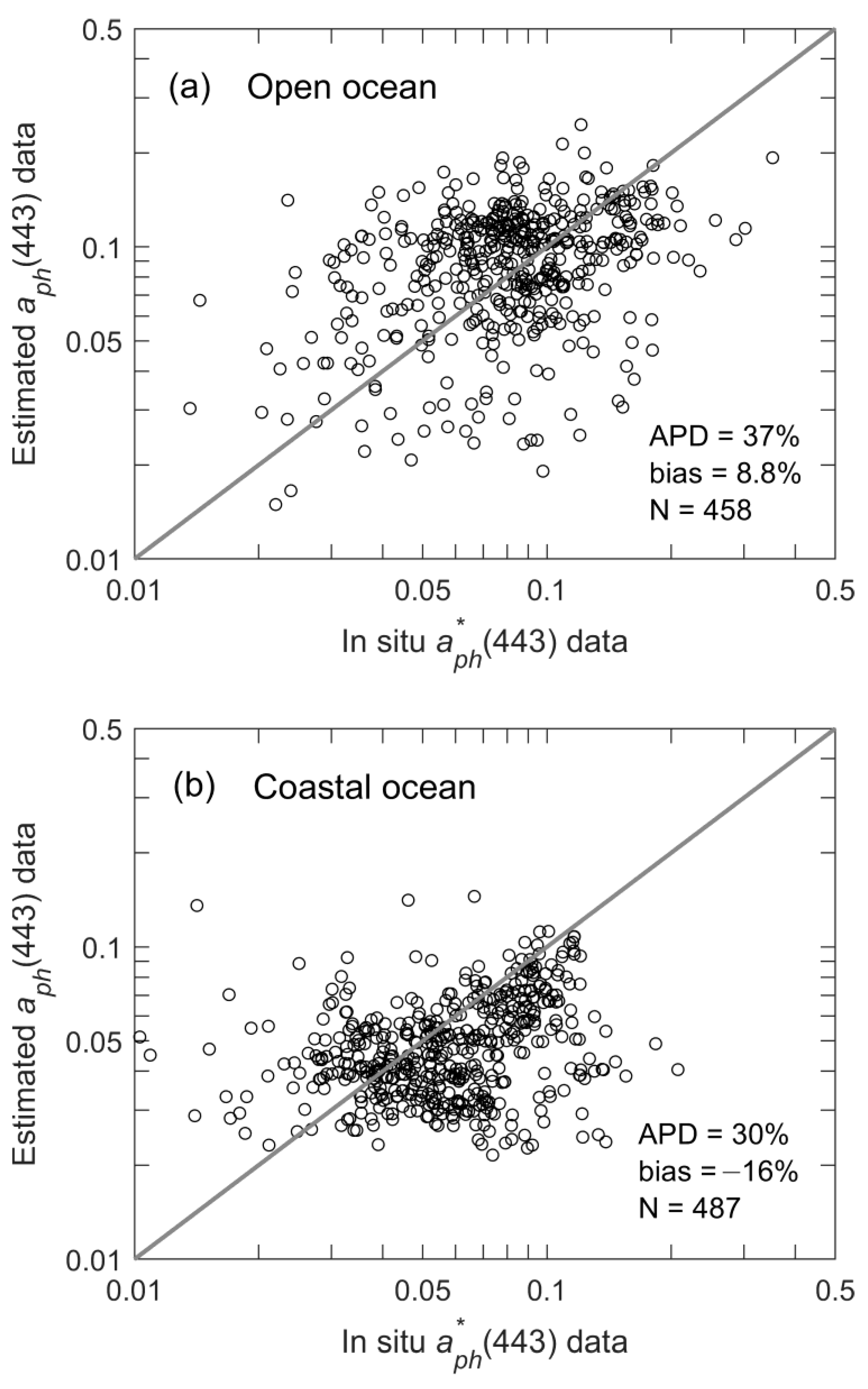
2.4. In Situ Data to Assist Evaluation

We retrieved in situ time series pigment measurements of surface water samples from the Hawaii Ocean Time-series (HOT) Aloha station (22.75°N, 158°W) for model evaluation. The pigment composition data were determined via HPLC. We reconstructed the phytoplankton absorption coefficient spectra from the HPLC pigments and the in vivo pigment absorption spectra following Bidigare et al. [16]. Then, we used the model of Woźniak et al. [60] to correct the light absorption data for the package effect (also see Letelier et al. [17] and Zoffoli et al. [61]). In addition, we accessed and included the Bermuda Atlantic Time Series (BATS) bio-optical data for comparison. According to the BATS program, the phytoplankton pigments were measured using the HPLC approach, and the phytoplankton absorption coefficient was determined using the quantitative filter technique (QFT) [62].

In addition to the above time series data, we also extracted phytoplankton Chl-a concentration and light absorption coefficient measurements from a compiled dataset [63] and the NASA SeaWiFS Bio-optical Archive and Storage System (SeaBASS) [64]. These data were recovered from discrete stations covering a variety of optical water types (Figure 1). The phytoplankton absorption measurement approaches were somewhat diverse but mostly followed the NASA-recommended protocols [65]. The pigment concentration data were generally determined via either HPLC or the fluorometric approach. In total, these two databases yielded 2576 matchups of phytoplankton absorption and pigment concentration data for the validation analysis.

The absolute percentage difference (APD) was derived as

$$\mathrm{APD}=\mathrm{median} \left[\left|\frac{P_i-M_i}{M_i}\right|\right]\times 100\%,$$

(7)

where P and M represent two quantities to be compared, with M being the reference and the subscript i referring to the sequence of data pairs. In analogy, the bias between P and M was evaluated as

$$\mathrm{bias}=\mathrm{median} [P_i-M_i] \times 100\%.$$

(8)

3. Results and Discussion

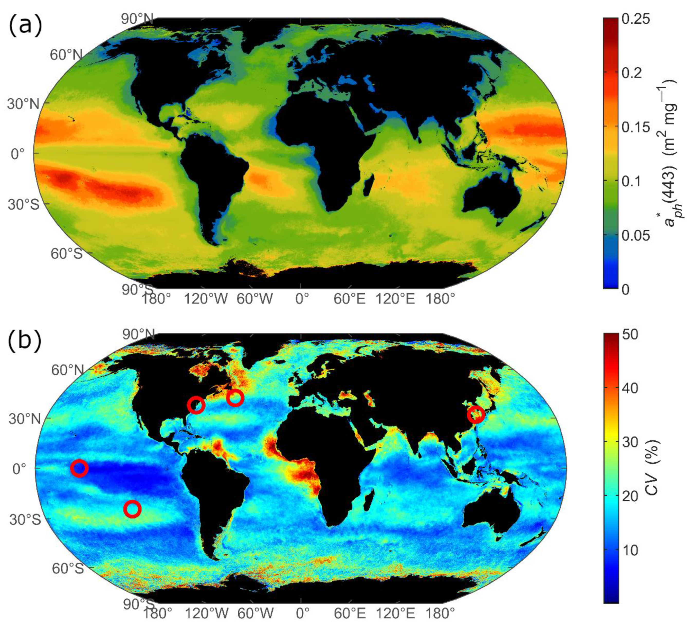
3.1. Spatial Distribution of Multi-Year Averages

The map of 4-year annual climatology describes the spatial feature of the chlorophyll-specific absorption coefficient of phytoplankton at 443 nm in the global ocean (Figure 2a). The median $a_{\mathit{ph}}^{*}(443)$ value for global open oceans is estimated to be 0.103 m² mg⁻¹ (standard deviation (STD) = 0.028 m² mg⁻¹). It is reduced by almost half and equal to 0.062 m² mg⁻¹ (STD = 0.026 m² mg⁻¹) within the coastal domain. The decreasing trend in $a_{\mathit{ph}}^{*}(443)$ from oligotrophic to mesotrophic/eutrophic oceans is opposite to that of Chl-a concentration, which, as is well known, remains the lowest in the central ocean basins and yet is abundant in coastal oceans [66].

Satellite observations revealed considerable spatial variance in $a_{\mathit{ph}}^{*}(443)$, with significant departures from the global median value. To illustrate this problem, we compared a selection of $a_{\mathit{ph}}^{*}(443)$ estimations across the ocean basins (

Table 1. Statistics of the regional mean chlorophyll-specific absorption coefficient of phytoplankton $a_{\mathit{ph}}^{*}(443)$ (unit: m² mg⁻¹) in the open and coastal oceans.

		Satellite Data (2014–2017)					In Situ Data
		Median	Min.	Max.	STD	CV	Range of Variation	Observation Time
Open Ocean	North Atlantic Gyre	0.114	0.090	0.141	0.015	13%	0.13 [72]	—
	South Atlantic Gyre	0.132	0.099	0.159	0.017	13%	—
	North Pacific Gyre	0.147	0.120	0.172	0.021	14%	0.070–0.140 [17]	January–December
	South Pacific Gyre	0.155	0.117	0.189	0.025	16%	0.070–0.100 [71]	October–December
	Indian Ocean Gyre	0.125	0.093	0.161	0.020	16%	—
	Equatorial Pacific	0.115	0.106	0.137	0.007	6%	0.080–0.130 [73]	November
	South China Sea	0.104	0.079	0.125	0.012	12%	—	—
	Gulf of Mexico	0.093	0.073	0.116	0.012	13%	—	—
	Mediterranean Sea	0.062	0.038	0.084	0.011	18%	0.023–0.165 [70]	September–November
Coastal Ocean	Baltic Sea	0.043	0.034	0.097	0.013	30%	0.016–0.124 [74]	March–May, August–October
	Black Sea	0.036	0.022	0.056	0.009	25%	0.030–0.115 [26]	August–September, November–December
	Gulf of Maine	0.048	0.036	0.110	0.016	33%	0.040–0.079 [75]	April, October
	Hudson Bay	0.048	0.031	0.170	0.034	71%	0.019–0.125 [76]	July, September–October
	Long Island Sound	0.035	0.023	0.058	0.010	29%	—	—
	Gulf of Mexico	0.054	0.040	0.079	0.009	17%	0.020–0.150 [77]	April–May, July–August, November
	Yellow Sea	0.045	0.023	0.062	0.010	22%	—	—

). Among them, the highly stratified oligotrophic waters within the subtropical ocean gyres stand out. On average, the South Pacific Gyre has the highest $a_{\mathit{ph}}^{*}(443)$ (~0.155 m² mg⁻¹), which is >35% higher than that of the North Atlantic Gyre and >25% higher than the Indian Ocean Gyre. Note that these gyre waters belong to the optical water type of Class 1 [4] and are known as “the ocean deserts” due to low Chl-a concentrations. The marked variances in $a_{\mathit{ph}}^{*}(443)$ across the subtropical ocean basins can be ascribed to the different pigment compositions and/or cell sizes of the phytoplankton species [67,68], which are further decided by the unique physical forcing and nutrient supply [66,69]. A second data group is representative of the Equatorial Pacific Ocean, South China Sea, Gulf of Mexico, and Mediterranean Sea, where the water types are dominantly Classes 2–3 [4]. Notably low $a_{\mathit{ph}}^{*}(443)$ values have been recorded in the Mediterranean Sea (~40% smaller on average than the other 3), which have been corroborated by the field observations and can be explained by its distinct regional phytoplankton features (pigment concentration, composition, and size) [70,71]. The coastal oceans exhibited considerable regional variances as well, despite the smaller absolute differences because of the relatively small $a_{\mathit{ph}}^{*}(443)$ values. However, due to the temporal variability, it is common for $a_{\mathit{ph}}^{*}(443)$ to experience a two-fold change in the coastal region. In contrast, the variability in $a_{\mathit{ph}}^{*}(443)$ is usually within 50% of the medians. Table 1 presents the medians, minima, maxima, and STDs of the regional data to reflect this problem. A pixel-by-pixel quantification of the temporal variation is shown in Figure 2b, where the coefficient of variation (CV) of $a_{\mathit{ph}}^{*}(443)$ was computed as the ratio of STD to the median specific absorption. It is common for $a_{\mathit{ph}}^{*}(443)$ to undergo variability with CV = 15–30% in open oceans and CV = 20–50% in coastal oceans.

The validation of the satellite-derived $a_{\mathit{ph}}^{*}(443)$ data remains difficult at this moment as it needs simultaneous matchups of in situ Chl-a and $a_{\mathit{ph}}(\lambda )$ measurements from the field campaigns that were conducted beneath the satellite overpass. We instead made a somewhat qualitative comparison of the range of variation between satellite data and existing in situ measurements. Table 1 presents the statistics for a selection of geographical regimes that were relatively easy to delineate from the surrounding environments. First, Morel et al. [72] measured the Prochlorococcus and Synechococcus cultures with a maximum of ~0.13 m² mg⁻¹ in the North Atlantic Gyre, which is close to the mean satellite observations. Letelier et al. [17] reported the maximum $a_{\mathit{ph}}^{*}(443)$ value of ~0.14 m² mg⁻¹ in the northwest of Hawaii, which is equivalent to our estimated median values. A few valuable measurements recovered from the South Pacific Gyre (~0.07–0.1 m² mg⁻¹) [71] approach the lower limits of the satellite observations, perhaps because the field data merely represented the situations occurring in October–December. Field observations from other open and coastal environments are further presented in Table 1, which are hard to compare with the satellite results for the seasonal variability.

3.2. Temporal Variation in Monthly $a_{\mathit{ph}}^{*}(443)$

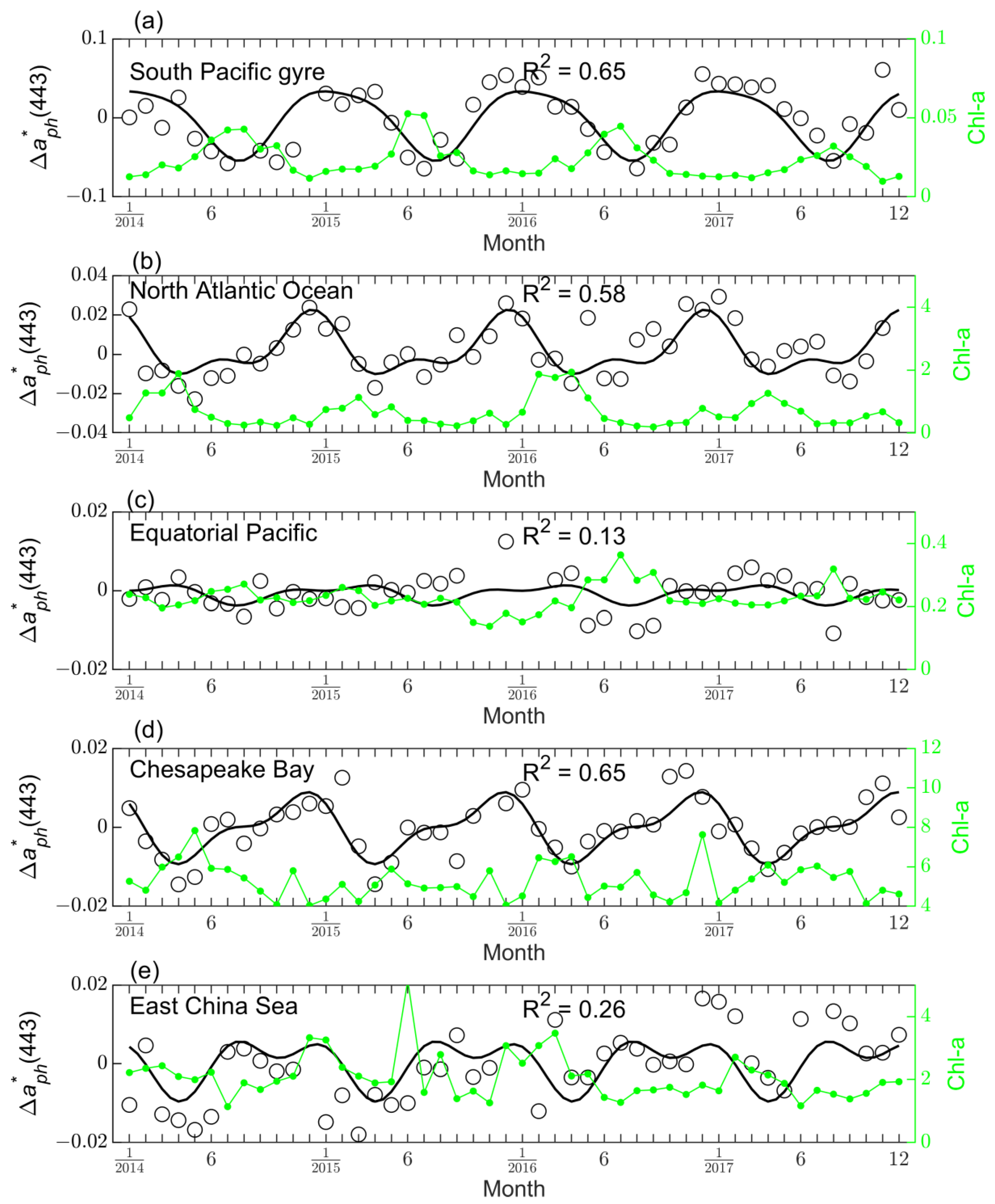
3.2.1. Example Time Series Data

We extracted 5 monthly time series data representative of distinct ocean physical and biogeochemical environments to demonstrate the periodical variations in the chlorophyll-specific absorption coefficient of phytoplankton at 443 nm. In Figure 3, the data points for the residual absorption $∆a_{\mathit{ph}}^{*}(443)$ are denoted as open circles, and the fitted curves are overlaid on top for comparison. The satellite monthly Chl-a data are also superimposed to elucidate its covariation with $a_{\mathit{ph}}^{*}(443)$. The South Pacific Gyre waters appear to have the most intense fluctuations despite having the least Chl-a concentration (Figure 3a). The differences between the maxima and minima are about 0.10 m² mg⁻¹. The annual minima (or maxima) occurred approximately simultaneously with the maxima (or minima) of Chl-a concentration. In the North Atlantic transition zone, the example data exhibit a primary peak during the fall–winter period and a secondary one in summer (Figure 3b). The associated annual minima correspond to the primary Chl-a peaks in springtime. The high coefficient of determination R² values (~0.6) in these 2 examples confirm the satisfactory performance of the sinusoidal model fitting. In the Equatorial Pacific Ocean, however, the specific absorption coefficient experienced weak periodical variations with the smallest amplitudes (Figure 3c) because nearly constant solar irradiation and nutrient supply resulted in relatively stable phytoplankton community structures [69]. The resulting model fit appears to be somewhat redundant in this scenario. Under this circumstance, one may predict this residual term for the specific absorption coefficient to be zero. It is observed that the model characterized the seasonal variability reasonably well in the coastal ocean example in Chesapeake Bay (R² = 0.65, Figure 3d), where minor and major peaks existed in summer and fall/winter, respectively. The example in Figure 3e was from an environment under significant terrestrial nutrient inputs and with a data shortage due to unfavorable atmospheric conditions. The resulting specific absorption data understandably deviated to an increased extent from otherwise more predictable periodic cycles (R² = 0.26).

3.2.2. Goodness of Fit

The model of Equation (5) was fitted to the monthly time series on a pixel-by-pixel basis. In Figure 4a, we use the coefficient of determination R² to quantify the appropriateness of the model fitting. With the prevalence of high R² over the vast oceans, it is evident that satisfactory regressions have been reached (with a mean R² of 0.45). Among others, the subtropical ocean gyres stand out with an average R² value of 0.6. At least half of the coastal oceans have R² values greater than 0.46. Small R² values are most common in the Pacific Ocean, consistent with the findings on the seasonal variability in Chl-a [78]. Small R² values also coincide with regions suffering from missing satellite observations due to clouds and heavy aerosols. Whereas the apparent $∆a_{\mathit{ph}}^{*}(443)$ time series over these waters might have been distorted due to insufficient data coverage, one cannot rule out the possibility that their actual seasonal variations may be close to the fitted sinusoidal patterns. In the vicinity of polar waters, especially beyond ±50° latitudes, many ocean color data are not valid because of unfavorable retrieval conditions, e.g., large solar-zenith angles, large sensor-zenith angles, high sun glint contamination, and cloud coverage [44,79], which are not included in the regressions.

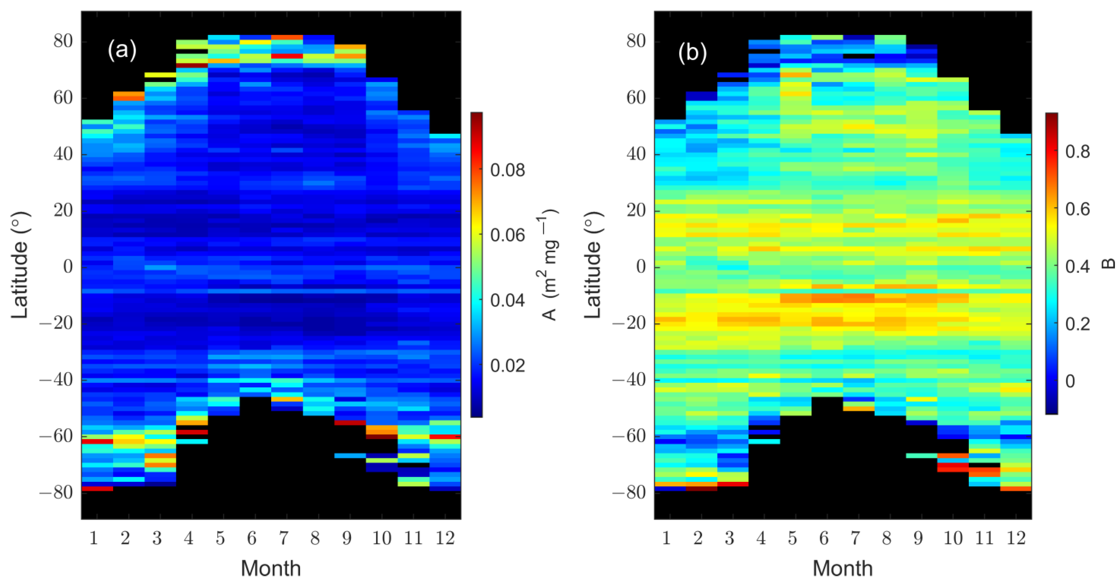
3.2.3. Seasonal Variability

We estimated the occurrence time for the seasonal maximum $a_{\mathit{ph}}^{*}(443)$ (denoted as T_max) from the fitted functions. As in Figure 4b, T_max exhibits a characteristic latitudinal dependence. The times at the corresponding latitudes in the northern and southern hemispheres are out of phase by approximately six months. For example, T_max in the North Pacific Subtropical Gyre occurs in July–September, while it happens in January–March in its southern counterpart (also see Figure 3a). The temperate regions in the North Atlantic witnessed maximum $a_{\mathit{ph}}^{*}(443)$ during November–January, right before the initiation of the spring blooms (also see Figure 3b). Correspondingly, maximum $a_{\mathit{ph}}^{*}(443)$ values occurred in May–July in the sub-Antarctic regions. The discovery of the latitudinal variation in T_max is analogous to the zonal characteristics of the ocean surface Chl-a concentration [57,78]. The latitudinal periodicity supports the fact that phytoplankton phenology is primarily driven by the seasonal cycles of solar radiation incident upon the ocean surface, which affects the intensity and timing of the water column stability and nutrient flux.

The annual and semiannual amplitudes are either positive or negative (Figure 4c,d), a result of the phase shifts in the global time series observations. As expected, the annual cycles are generally much more substantial than the semiannual signals, with ${|a}_1|\gg |a_2|$, suggesting dominance in the seasonal variations. Values of ${|a}_1|$ can be as high as 0.04–0.05 m² mg⁻¹ in the open ocean, especially in the subtropical gyres. For the annual component, the signs of the amplitudes are alternatively changing along the latitudinal direction. For example, negative and positive amplitudes are present in the subtropics of the northern and southern hemispheres (±5°–35° latitude), respectively. Regarding higher latitudes, the amplitudes transitioned to positive and negative values in the temperate of the northern hemisphere and southern hemisphere (±35°–50° latitude), respectively. These primary cycles in the northern and southern hemispheres are essentially 180° (or 6 months) out of phase. In contrast, the amplitude of the semiannual component $a_2$ appears to be approximately symmetric about the equator with opposite signs. The presence of relatively high ${|a}_2|$ values appears to coincide with two phytoplankton blooms often prevailing in monthly time series data, including the North Atlantic Ocean [80], the Arabian Sea [81], and the Equatorial Atlantic Ocean [82].

Cross-correlation analysis of the monthly $a_{\mathit{ph}}^{*}(443)$ and Chl-a time series did not reveal significant lags between the timing of maximum Chl-a and minimum $a_{\mathit{ph}}^{*}(443)$ in global oceans. Note that the dominant pigments varied seasonally and geographically [30]. The intracellular pigments, including Chl-a and the accessory chlorophylls, photosynthetic carotenoids, and photoprotective carotenoids, all absorb light. Thus, it is still possible for the existence of a time lag between Chl-a and $a_{\mathit{ph}}^{*}(443)$ in nature. However, if the time lags were shorter than one month, it would be impossible to detect them from the present monthly data. On the other hand, ocean color algorithms rely mainly on the spectral shapes of the ocean color spectra, which might have suppressed the time lags.

3.3. Dependence of $a_{\mathit{ph}}^{*}(443)$ on Chl-a Concentration

We examined the global relationship between $a_{\mathit{ph}}^{*}(443)$ and Chl-a using satellite-derived climatological data. As shown in Figure 5, the chlorophyll-specific absorption is inversely reliant on Chl-a concentration, reflecting the package effect [6,7]. The log10-transformed $a_{\mathit{ph}}^{*}(443)$ and Chl-a data form a close-to-ideal linear relationship, which can be described sufficiently by the power model (R² = 0.99), $a_{\mathit{ph}}^{*}(443)=0.05672·{\left[\mathrm{Chl-a}\right]}^{-0.3051}$. We compared this global relationship with the model fit made to the NOMAD data and with the original work of Bricaud et al. [6]. Specifically, the regression to the NOMAD data gives rise to a power function with A = 0.0547 m² mg⁻¹, which is almost the same as our global model, and B = 0.2526, slightly smaller than our result. In contrast, the Bricaud et al. [6] model departs from our global model with a smaller coefficient A = 0.0398 m² mg⁻¹, but has a coefficient of B = 0.339 which is very close to our global estimates. Overall, the disparities among these three scenarios are acceptably close to each other, inasmuch as the three datasets represented different geographical and seasonal features.

We further assessed the $a_{\mathit{ph}}^{*}(443)$ and Chl-a relationship with respect to latitudes and seasons based on satellite-derived monthly climatology data. The analyses revealed geographical and seasonal dependences of $a_{\mathit{ph}}^{*}(443)$ on Chl-a, with the model coefficients varying over wide ranges and sometimes deviating significantly from the global mean relationship. As indicated in Figure 6a, for example, moderate A values (<0.04 m² mg⁻¹) are present in the northern subtropical oceans (~15°–40°N) and southern subtropical oceans (~10°–30°S). In the temperate and subarctic regions, large A values are easily spotted that exceed 0.07 m² mg⁻¹. Most B values are limited to 0.2–0.6 over the vast oceans but remain the highest in the subtropics. It is also evident that both A and B coefficients experienced non-negligible seasonal variability. For example, the values of A at 40°N increased by a factor of 1.5 when transitioning from summer to winter. At the same time, the corresponding B values dropped from >0.5 to <0.3. These regional and seasonal variations in the model coefficients echo the field observations occurring in different parts of the world ocean [9,25,27,83,84]. However, comparing the coefficients A and B in Figure 6 with earlier field observations is not straightforward because of differing data ranges and ocean provinces being focused on during respective analyses. The seasonal/regional dependency of the phytoplankton absorption on Chl-a probably arises from the zonal changes in the cell size structure and taxonomic composition of phytoplankton communities (e.g., [68]), which are ultimately decided by the solar radiation upon ocean surfaces.

3.4. Estimation of $a_{\mathit{ph}}^{*}(443)$ as a Function of Geolocation and Time

As a critical element of ocean color applications, $a_{\mathit{ph}}^{*}(\lambda )$ is often modeled as a function of phytoplankton pigment concentrations [6,23,24,85]. As discovered in this study, the seasonal and regional dependence of $a_{\mathit{ph}}^{*}(\lambda )$ on pigment concentrations will complicate the practices relying on global relationships. Can the new seasonal/regional results presented so far be further exploited to fulfill the synoptic prediction of the phytoplankton absorption for global applications? They certainly can. In fact, the paradigm of $a_{\mathit{ph}}^{*}(\lambda )$ time series data presents an alternative for predicting $a_{\mathit{ph}}^{*}(443)$ as the sum of the means and the seasonal residuals,

$$a_{\mathit{ph}}^{*}(443)=\overline{a_{\mathit{ph}}^{*}}(443)+∆a_{\mathit{ph}}^{*}(443),$$

(9)

where $\overline{a_{\mathit{ph}}^{*}}(443)$ refers to long-term climatology and can be adopted from Figure 2. The time-dependent $∆a_{\mathit{ph}}^{*}(443)$ is modeled by Equation (5), with the coefficients $a_1$, $a_2$, ${\phi }_1$, and ${\phi }_2$ ($a_0$ is not essential) determined using the satellite data fitting. Thus, the chlorophyll-specific absorption coefficient of phytoplankton at 443 nm can be approximated as a function of geolocation and time, independent of Chl-a measurements.

We tested this hypothesis with in situ time series measurements collected from Hawaii and Bermuda. As shown in Figure 7, an overall agreement is reached between in situ and estimated $∆a_{\mathit{ph}}^{*}(443)$. The model data pairs differ by an absolute percentage difference APD = 18.2% in Hawaii (and bias > 200%). For the Bermuda data, the estimations have an APD of 15.1% (and bias = 120%). Note that the significant biases are partially ascribed to the small absolute values of $∆a_{\mathit{ph}}^{*}(443)$ relative to their climatology means. Moreover, we cannot dismiss the possibility that in situ data are not free of measurement uncertainties [86]. Nonetheless, the estimated and in situ $∆a_{\mathit{ph}}^{*}(443)$ data are significantly correlated, with R² = 0.92 and R² = 0.69 for Hawaii and Bermuda data, respectively.

Figure 8 compares the model-estimated $a_{\mathit{ph}}^{*}(443)$ with in situ measurements at discrete stations around the global ocean. As far as the open ocean data are concerned, the model yields $a_{\mathit{ph}}^{*}(443)$ with high accuracy, where APD = 37% and bias = 8.8%. For coastal ocean data, the model estimates $a_{\mathit{ph}}^{*}(443)$ with APD = 30% and bias = −16%. Notably, an uncertainty of ~30–40% is acceptably small and is comparable with that of satellite-retrieved Chl-a products in open oceans (~30%) (e.g., [87]). It is also important to emphasize that the model tested here works more appropriately for predicting monthly $a_{\mathit{ph}}^{*}(443)$ and does not sufficiently represent the daily variation in $a_{\mathit{ph}}^{*}(443)$, nor does the model account for diurnal variability in this bio-optical quantity. The in situ data used for this comparison were measured on specific days. These discrepancies can partially explain the scatters seen in the plots. In addition, the measuring and processing procedures of water samples for $a_{\mathit{ph}}(443)$ were different among cruises and investigators, which unavoidably resulted in measurement uncertainties for $a_{\mathit{ph}}(443)$ [86]. Finally, although the model data deviations are small in Figure 8, cautious practices are recommended in light of the ocean’s dynamic nature. For example, ocean phytoplankton can undergo abnormal changes in biomass during an El Niño Southern Oscillation (ENSO) period [88], and the community structure shifts after episodic events [89]. Nonetheless, the above analyses demonstrated an independent procedure for the prediction of the phytoplankton absorption over global oceans, a promising approach for synoptic remote sensing and large-scale ocean modeling.

4. Conclusions

Based on satellite observations, this article has explored the seasonal and regional variability in the chlorophyll-specific absorption coefficient of phytoplankton at 443 nm $a_{\mathit{ph}}^{*}(443)$ in global oceans. The analyses revealed considerable spatial variance in the long-term climatology of the specific absorption across global oceans. Our data also showed substantial seasonal variability in $a_{\mathit{ph}}^{*}(443)$ around the median values. The coefficient of variation can be as high as 100% in coastal oceans and 30% in open oceans. Using a model-fitting approach, we characterized the zonal distribution of the amplitudes in the monthly time series and the occurrence time of the maximum $a_{\mathit{ph}}^{*}(443)$. The seasonal patterns in the open oceans of the northern hemisphere are primarily opposite to those of the southern hemisphere, suggesting a significant latitudinal dependence. We further examined and verified that a simple analytical model, with the model coefficients derived from the regressions of satellite data, can indeed predict the complex seasonal signals of the chlorophyll-specific absorption coefficient of phytoplankton at 443 nm with an absolute percentage error of ~30% on average. It is also pointed out that although the seasonal variations in $a_{\mathit{ph}}^{*}(443)$ are concomitant with corresponding differences in Chl-a, the dependence of $a_{\mathit{ph}}^{*}(443)$ on Chl-a is subjected to seasonal and regional variability. We argue that the analytical model tested in this study can act as an alternative approach for estimating chlorophyll-specific absorption. In particular, this approach is relatively independent and does not demand information on the phytoplankton pigment concentrations.

The present analyses are based on the monthly $a_{\mathit{ph}}^{*}(443)$ data and apply to monthly schemes most appropriately. The resulting model does not sufficiently depict the data at a finer temporal interval, such as the daily data. This problem can be circumvented in the future by adopting gap-free ocean color products in which the data loss associated with the cloudiness and the width of the satellite image swath are compensated [90,91]. Another limitation resides in the single wavelength discussed in the context. The red band of 671 nm is omitted from this study because the current satellite ocean color retrievals at this band are subjected to large uncertainties in open oceans because the absolute values are too small. Future attempts should include $a_{\mathit{ph}}^{*}(\lambda )$ at the red band for a complete perspective of the spectral variability in the chlorophyll-specific absorption coefficient of phytoplankton, particularly over turbid coastal and inland waters.

References

1. Siegel, D.A.; Buesseler, K.O.; Doney, S.C.; Sailley, S.F.; Behrenfeld, M.J.; Boyd, P.W. Global assessment of ocean carbon export by combining satellite observations and food-web models. Global Biogeochem. Cycles 2014, 28, 181–196. [Google Scholar] [CrossRef]
2. Platt, T.; Sathyendranath, S.; Forget, M.-H.; White, G.N., III; Caverhill, C.; Bouman, H.; Devred, E.; Son, S. Operational estimation of primary production at large geographical scales. Remote. Sens. Environ. 2008, 112, 3437–3448. [Google Scholar] [CrossRef]
3. Hoepffner, N.; Sathyendranath, S. Effect of pigment composition on absorption properties of phytoplankton. Mar. Ecol. Prog. Ser. 1991, 73, 11–23. [Google Scholar] [CrossRef]
4. Wei, J.; Wang, M.; Mikelsons, K.; Jiang, L.; Kratzer, S.; Lee, Z.P.; Moore, T.; Sosik, H.M.; Van der Zande, D. Global satellite water classification data products over oceanic, coastal, and inland waters. Remote. Sens. Environ. 2022, 282, 113233. [Google Scholar] [CrossRef]
5. Prieur, L.; Sathyendranath, S. An optical classification of coastal and oceanic waters based on the specific spectral absorption curves of phytoplankton pigments, dissolved organic matter, and other particulate materials. Limnol. Oceanogr. 1981, 26, 671–689. [Google Scholar] [CrossRef]
6. Bricaud, A.; Babin, M.; Morel, A.; Claustre, H. Variability in the chlorophyll-specific absorption coefficients of natural phytoplankton: Analysis and parameterization. J. Geophys. Res. 1995, 100, 13321–13332. [Google Scholar] [CrossRef]
7. Bricaud, A.; Morel, A.; Babin, M.; Allali, K.; Claustre, H. Variations of light absorption by suspended particles with chlorophyll a concentration in oceanic (case 1) waters: Analysis and implications for bio-optical models. J. Geophys. Res. 1998, 103, 31033–31044. [Google Scholar] [CrossRef]
8. Babin, M.; Stramski, D.; Ferrari, G.M.; Claustre, H.; Bricaud, A.; Obolensky, G.; Hoepffner, N. Variations in the light absorption coefficients of phytoplankton, nonalgal particles, and dissolved organic matter in coastal waters around Europe. J. Geophys. Res. 2003, 108, 3211. [Google Scholar] [CrossRef]
9. Cleveland, J.S. Regional models for phytoplankton absorption as a function of chlorophyll a concentration. J. Geophys. Res. 1995, 100, 13333–13344. [Google Scholar] [CrossRef]
10. Werdell, P.J.; Franz, B.A.; Bailey, S.W.; Feldman, G.C.; Boss, E.; Brando, V.E.; Dowell, M.; Hirata, T.; Lavender, S.J.; Lee, Z.P.; et al. Generalized ocean color inversion model for retrieving marine inherent optical properties. Appl. Opt. 2013, 52, 2019–2037. [Google Scholar] [CrossRef] [PubMed]
11. Tilstone, G.H.; Peters, S.W.M.; van der Woerd, H.J.; Eleveld, M.A.; Ruddick, K.; Schönfeld, W.; Krasemann, H.; Martinez-Vicente, V.; Blondeau-Patissier, D.; Röttgers, R.; et al. Variability in specific-absorption properties and their use in a semi-analytical ocean colour algorithm for MERIS in North Sea and Western English Channel Coastal Waters. Remote. Sens. Environ. 2012, 118, 320–338. [Google Scholar] [CrossRef]
12. Zheng, G.; DiGiacomo, P.M. Remote sensing of chlorophyll-a in coastal waters based on the light absorption coefficient of phytoplankton. Remote. Sens. Environ. 2017, 201, 331–341. [Google Scholar] [CrossRef]
13. Carder, K.L.; Chen, F.R.; Lee, Z.P.; Hawes, S.K.; Kamykowski, D. Semianalytic Moderate-resolution Imaging Spectrometer algorithms for chlorophyll-a and absorption with bio-optical domains based on nitrate-depletion temperatures. J. Geophys. Res. 1999, 104, 5403–5421. [Google Scholar] [CrossRef]
14. Morel, A. Light and marine photosynthesis: A spectral model with geochemical and climatological implications. Prog. Oceanogr. 1991, 26, 263–306. [Google Scholar] [CrossRef]
15. Uitz, J.; Claustre, H.; Gentili, B.; Stramski, D. Phytoplankton class-specific primary production in the world's oceans: Seasonal and interannual variability from satellite observations. Global Biogeochem. Cycles 2010, 24, GB3016. [Google Scholar] [CrossRef]
16. Bidigare, R.R.; Ondrusek, M.E.; Morrow, J.H.; Kiefer, D.A. In vivo absorption properties of algal pigments. In Ocean Optics X; Society of Photo Optical: Bellingham, WA, USA, 1990; pp. 290–302. [Google Scholar]
17. Letelier, R.M.; White, A.E.; Bidigare, R.R.; Barone, B.; Church, M.J.; Karl, D.M. Light absorption by phytoplankton in the North Pacific Subtropical Gyre. Limnol. Oceanogr. 2017, 62, 1526–1540. [Google Scholar] [CrossRef]
18. Liu, Y.; Boss, E.; Chase, A.; Xi, H.; Zhang, X.; Röttgers, R.; Pan, Y.; Bracher, A. Retrieval of phytoplankton pigments from underway spectrophotometry in the Fram Strait. Remote. Sens. 2019, 11, 318. [Google Scholar] [CrossRef]
19. Moisan, T.A.; Rufty, K.M.; Moisan, J.R.; Linkswiler, M.A. Satellite observations of phytoplankton functional type spatial distributions, phenology, diversity, and ecotones. Front. Mar. Sci. 2017, 4, 189. [Google Scholar] [CrossRef]
20. Ciotti, A.M.; Bricaud, A. Retrievals of a size parameter for phytoplankton and spectral light absorption by colored detrital matter from water-leaving radiances at SeaWiFS channels in a continental shelf region off Brazil. Limnol. Oceanogr. Methods 2006, 4, 237–253. [Google Scholar] [CrossRef]
21. Roy, S.; Sathyendranath, S.; Bouman, H.; Platt, T. The global distribution of phytoplankton size spectrum and size classes from their light-absorption spectra derived from satellite data. Remote. Sens. Environ. 2013, 139, 185–197. [Google Scholar] [CrossRef]
22. Zhou, W.; Wang, G.; Li, C.; Xu, Z.; Cao, W.; Shen, F. Retrieval of phytoplankton cell size from chlorophyll a specific absorption and scattering spectra of phytoplankton. Appl. Opt. 2017, 56, 8362–8371. [Google Scholar] [CrossRef] [PubMed]
23. Brewin, R.J.W.; Devred, E.; Sathyendranath, S.; Lavender, S.J.; Hardman-Mountford, N.J. Model of phytoplankton absorption based on three size classes. Appl. Opt. 2011, 50, 4535–4549. [Google Scholar] [CrossRef]
24. Uitz, J.; Huot, Y.; Bruyant, F.; Babin, M.; Claustre, H. Relating phytoplankton photophysiological properties to community structure on large scales. Limnol. Oceanogr. 2008, 53, 614–630. [Google Scholar] [CrossRef]
25. Devred, E.; Perry, T.; Massicotte, P. Seasonal and decadal variations in absorption properties of phytoplankton and non-algal particulate matter in three oceanic regimes of the Northwest Atlantic. Front. Mar. Sci. 2022, 9, 932184. [Google Scholar] [CrossRef]
26. Churilova, T.; Suslin, V.; Krivenko, O.; Efimova, T.; Moiseeva, N.; Mukhanov, V.; Smirnova, L. Light absorption by phytoplankton in the upper mixed layer of the Black Sea: Seasonality and parametrization. Front. Mar. Sci. 2017, 4, 90. [Google Scholar] [CrossRef]
27. Mercado, J.M.; Gómez-Jakobsen, F. Seasonal variability in phytoplankton light absorption properties: Implications for the regional parameterization of the chlorophyll a specific absorption coefficients. Cont. Shelf Res. 2022, 232, 104614. [Google Scholar] [CrossRef]
28. Matsuoka, A.; Hill, V.; Huot, Y.; Babin, M.; Bricaud, A. Seasonal variability in the light absorption properties of western Arctic waters: Parameterization of the individual components of absorption for ocean color applications. J. Geophys. Res. Ocean. 2011, 116, C02007. [Google Scholar] [CrossRef]
29. Sasaki, H.; Miyamura, T.; Saitoh, S.-I.; Ishizaka, J. Seasonal variation of absorption by particles and colored dissolved organic matter (CDOM) in Funka Bay, southwestern Hokkaido, Japan. Estuar. Coast. Shelf Sci. 2005, 64, 447–458. [Google Scholar] [CrossRef]
30. Sathyendranath, S.; Stuart, V.; Irwin, B.D.; Maass, H.; Savidge, G.; Gilpin, L.; Platt, T. Seasonal variations in bio-optical properties of phytoplankton in the Arabian Sea. Deep Sea Res. Part II Top. Stud. Oceanogr. 1999, 46, 633–653. [Google Scholar] [CrossRef]
31. Lorenzoni, L.; Hu, C.; Varela, R.; Arias, G.; Guzmán, L.; Muller-Karger, F. Bio-optical characteristics of Cariaco Basin (Caribbean Sea) waters. Cont. Shelf Res. 2011, 31, 582–593. [Google Scholar] [CrossRef]
32. Wang, M.; Liu, X.; Jiang, L.; Son, S. The VIIRS ocean color product algorithm theoretical basis document version 1.0. In NOAA NESDIS STAR Algorithm Theoretical Basis Document (ATBD); NOAA NESDIS Center for Satellite Applications and Research: Silver Spring, MD, USA, 2017; p. 68. [Google Scholar]
33. Wang, M.; Liu, X.; Tan, L.; Jiang, L.; Son, S.; Shi, W.; Rausch, K.; Voss, K.J. Impacts of VIIRS SDR performance on ocean color products. J. Geophys. Res. 2013, 118, 10347–10360. [Google Scholar] [CrossRef]
34. Gordon, H.R.; Wang, M. Retrieval of water-leaving radiance and aerosol optical thickness over the oceans with SeaWiFS: A preliminary algorithm. Appl. Opt. 1994, 33, 443–452. [Google Scholar] [CrossRef] [PubMed]
35. Wang, M. Remote sensing of the ocean contributions from ultraviolet to near-infrared using the shortwave infrared bands: Simulations. Appl. Opt. 2007, 46, 1535–1547. [Google Scholar] [CrossRef]
36. IOCCG. Atmospheric Correction for Remotely-Sensed Ocean Color Products, 10th ed.; International Ocean Color Coordinating Group: Dartmouth, NS, Canada, 2010; p. 78. [Google Scholar]
37. Jiang, L.; Wang, M. Improved near-infrared ocean reflectance correction algorithm for satellite ocean color data processing. Opt. Express 2014, 22, 21657–21678. [Google Scholar] [CrossRef] [PubMed]
38. Shi, W.; Wang, M. Ocean reflectance spectra at the red, near-infrared, and shortwave infrared from highly turbid waters: A study in the Bohai Sea, Yellow Sea, and East China Sea. Limnol. Oceanogr. 2014, 59, 427–444. [Google Scholar] [CrossRef]
39. Wang, M.; Shi, W. The NIR-SWIR combined atmospheric correction approach for MODIS ocean color data processing. Opt. Express 2007, 15, 15722–15733. [Google Scholar] [CrossRef] [PubMed]
40. Wei, J.; Wang, M.; Ondrusek, M.; Gilerson, A.; Goes, J.; Hu, C.; Lee, Z.; Voss, K.J.; Ladner, S.; Lance, V.P.; et al. Satellite ocean color validation. In Field Measurements for Passive Environmental Remote Sensing: Instrumentation, Intensive Campaigns, and Satellite Applications; Nalli, N., Ed.; Elsevier: Cambridge, MA, USA, 2022; pp. 351–374. [Google Scholar]
41. Wei, J.; Yu, X.; Lee, Z.P.; Wang, M.; Jiang, L. Improving low-quality satellite remote sensing reflectance at blue bands over coastal and inland waters. Remote. Sens. Environ. 2020, 250, 112029. [Google Scholar] [CrossRef]
42. Hlaing, S.; Harmel, T.; Gilerson, A.; Foster, R.; Weidemann, A.D.; Arnone, R.; Wang, M.; Ahmed, S. Evaluation of the VIIRS ocean color monitoring performance in coastal regions. Remote. Sens. Environ. 2013, 139, 398–414. [Google Scholar] [CrossRef]
43. Ondrusek, M.; Wei, J.; Wang, M.; Stengel, E.; Kovach, C.; Gilerson, A.; Herrera, E.; Malinowski, M.; Goes, J.I.; Gomes, H.d.R.; et al. Report for dedicated JPSS VIIRS ocean color calibration/validation cruise: Gulf of Mexico in April 2021. In NOAA Technical Report NESDIS 157; NOAA National Environmental Satellite, Data Information, Service: Washington, DC, USA, 2022; p. 51. [Google Scholar]
44. Mikelsons, K.; Wang, M.; Jiang, L. Statistical evaluation of satellite ocean color data retrievals. Remote. Sens. Environ. 2020, 237, 111601. [Google Scholar] [CrossRef]
45. Hu, C.; Barnes, B.B.; Feng, L.; Wang, M.; Jiang, L. On the interplay between ocean color data quality and data quantity: Impacts of quality control flags. IEEE Geosci. Remote. Sens. Lett. 2020, 17, 745–749. [Google Scholar] [CrossRef]
46. Barnes, B.B.; Cannizzaro, J.P.; English, D.C.; Hu, C. Validation of VIIRS and MODIS reflectance data in coastal and oceanic waters: An assessment of methods. Remote. Sens. Environ. 2019, 220, 110–123. [Google Scholar] [CrossRef]
47. Wang, M.; Shi, W.; Watanabe, S. Satellite-measured water properties in high altitude Lake Tahoe. Water Res. 2020, 178, 115839. [Google Scholar] [CrossRef] [PubMed]
48. Wang, M.; Son, S. VIIRS-derived chlorophyll-a using the ocean color index method. Remote. Sens. Environ. 2016, 182, 141–149. [Google Scholar] [CrossRef]
49. Hu, C.; Lee, Z.P.; Franz, B. Chlorophyll a algorithms for oligotrophic oceans: A novel approach based on three-band reflectance difference. J. Geophys. Res. 2012, 117, 2156–2202. [Google Scholar] [CrossRef]
50. Shi, W.; Wang, M. A blended inherent optical property algorithm for global satellite ocean color observations. Limnol. Oceanogr. Methods 2019, 17, 377–394. [Google Scholar] [CrossRef]
51. Lee, Z.P.; Carder, K.L.; Arnone, R. Deriving inherent optical properties from water color: A multi-band quasi-analytical algorithm for optically deep waters. Appl. Opt. 2002, 41, 5755–5772. [Google Scholar] [CrossRef]
52. Gordon, H.R.; Brown, O.B.; Evans, R.H.; Brown, J.W.; Smith, R.C.; Baker, K.S.; Clark, D.K. A semianalytic radiance model of ocean color. J. Geophys. Res. 1988, 93, 10909–10924. [Google Scholar] [CrossRef]
53. IOCCG. Remote Sensing of Inherent Optical Properties: Fundamentals, Tests of Algorithms, and Applications, 5th ed.; International Ocean Color Coordinating Group: Dartmouth, NS, Canada, 2006; p. 126. [Google Scholar]
54. Campbell, J.W.; Blaisdell, J.M.; Darzi, M. Level-3 SeaWiFS Data Products: Spatial and Temporal Binning Algorithms; NASA Goddard Space Flight Center: Greenbelt, MD, USA, 1995; p. 104566. [Google Scholar]
55. Moisan, J.R.; Moisan, T.A.H.; Linkswiler, M.A. An inverse modeling approach to estimating phytoplankton pigment concentrations from phytoplankton absorption spectra. J. Geophys. Res. -Ocean. 2011, 116, C09018. [Google Scholar] [CrossRef]
56. Demarcq, H.; Reygondeau, G.; Alvain, S.; Vantrepotte, V. Monitoring marine phytoplankton seasonality from space. Remote. Sens. Environ. 2012, 117, 211–222. [Google Scholar] [CrossRef]
57. Dandonneau, Y.; Deschamps, P.-Y.; Nicolas, J.-M.; Loisel, H.; Blanchot, J.; Montel, Y.; Thieuleux, F.; Bécu, G. Seasonal and interannual variability of ocean color and composition of phytoplankton communities in the North Atlantic, equatorial Pacific and South Pacific. Deep Sea Res. Part II Top. Stud. Oceanogr. 2004, 51, 303–318. [Google Scholar] [CrossRef]
58. Mao, Z.; Mao, Z.; Jamet, C.; Linderman, M.; Wang, Y.; Chen, X. Seasonal cycles of phytoplankton expressed by sine equations using the daily climatology from satellite-retrieved chlorophyll-a concentration (1997–2019) over global ocean. Remote. Sens. 2020, 12, 2662. [Google Scholar] [CrossRef]
59. Yoder, J.A.; O'Reilly, J.E.; Barnard, A.H.; Moore, T.S.; Ruhsam, C.M. Variability in coastal zone color scanner (CZCS) Chlorophyll imagery of ocean margin waters off the US East Coast. Cont. Shelf Res. 2001, 21, 1191–1218. [Google Scholar] [CrossRef]
60. Woźniak, B.; Dera, J.; Ficek, D.; Majchrowski, R.; Kaczmarek, S.; Ostrowska, M.; Koblentz-Mishke, O.I. Modelling the influence of acclimation on the absorption properties of marine phytoplankton. Oceanologia 1999, 41, 187–210. [Google Scholar]
61. Zoffoli, M.L.; Lee, Z.; Marra, J.F. Regionalization and dynamic parameterization of quantum yield of photosynthesis to improve the ocean primary production estimates from remote sensing. Front. Mar. Sci. 2018, 5, 446. [Google Scholar] [CrossRef]
62. Mitchell, B.G.; Bricaud, A.; Carder, K.L.; Cleveland, J.; Ferrari, G.M.; Gould, R.; Kahru, M.; Kishino, M.; Maske, H.; Moisan, T.; et al. Determination of Spectral Absorption Coefficients of Particles, Dissolved Material, and Phytoplankton for Discrete Water Samples; Goddard Space Flight Center, NASA: Greenbelt, MA, USA, 2000; pp. 125–153. [Google Scholar]
63. Valente, A.; Sathyendranath, S.; Brotas, V.; Groom, S.; Grant, M.; Taberner, M.; Antoine, D.; Arnone, R.; Balch, W.M.; Barker, K.; et al. A compilation of global bio-optical in situ data for ocean-colour satellite applications—Version two. Earth Syst. Sci. Data 2019, 11, 1037–1068. [Google Scholar] [CrossRef]
64. Werdell, J.; Bailey, S.W. The SeaWiFS Bio-Optical Archive and Storage System (SeaBASS): Current Architecture and Implementation; NASA/TM-2002-211617; Goddard Space Flight Center: Greenbelt, MD, USA, 2002. [Google Scholar]
65. Mueller, J.; Fargion, G.; McClain, C.R. Ocean Optics Protocols for Satellite Ocean Color Validation, Revision 4, Volume IV: Inherent Optical Properties: Instruments, Characterizations, Field Measurements and Data Analysis Protocols; NASA: Greenbelt, MD, USA, 2003; p. 76. [Google Scholar]
66. McClain, C.R.; Signorini, S.R.; Christian, J.R. Subtropical gyre variability observed by ocean-color satellites. Deep-Sea Res. Part II 2004, 51, 281–301. [Google Scholar] [CrossRef]
67. Barlow, R.; Stuart, V.; Lutz, V.; Sessions, H.; Sathyendranath, S.; Platt, T.; Kyewalyanga, M.; Clementson, L.; Fukasawa, M.; Watanabe, S.; et al. Seasonal pigment patterns of surface phytoplankton in the subtropical southern hemisphere. Deep Sea Res. Part I Oceanogr. Res. Pap. 2007, 54, 1687–1703. [Google Scholar] [CrossRef]
68. Alvain, S.; Moulin, C.; Dandonneau, Y.; Loisel, H. Seasonal distribution and succession of dominant phytoplankton groups in the global ocean: A satellite view. Glob. Biogeochem Cycles 2008, 22, GB3001. [Google Scholar] [CrossRef]
69. Longhurst, A. Ecological Geography of the Sea; Academic Press: San Diego, CA, USA, 1998; p. 398. [Google Scholar]
70. Organelli, E.; Nuccio, C.; Melillo, C.; Massi, L. Relationships between phytoplankton light absorption, pigment composition and size structure in offshore areas of the Mediterranean Sea. Adv. Oceanogr. Limnol. 2011, 2, 107–123. [Google Scholar] [CrossRef]
71. Bricaud, A.; Babin, M.; Claustre, H.; Ras, J.; Tieche, F. Light absorption properties and absorption budget of Southeast Pacific waters. J. Geophys. Res. 2010, 115, C08009. [Google Scholar] [CrossRef]
72. Morel, A.; Ahn, Y.-H.; Partensky, F.; Vaulot, D.; Claustre, H. Prochlorococcus and Synechococcus: A comparative study of their optical properties in relation to their size and pigmentation. J. Mar. Res. 1993, 51, 617–649. [Google Scholar] [CrossRef]
73. Allali, K.; Bricaud, A.; Claustre, H. Spatial variations in the chlorophyll-specific absorption coefficients of phytoplankton and photosynthetically active pigments in the equatorial Pacific. J. Geophys. Res. 1997, 102, 12413–12423. [Google Scholar] [CrossRef]
74. Meler, J.; Ostrowska, M.; Ficek, D.; Zdun, A. Light absorption by phytoplankton in the southern Baltic and Pomeranian lakes: Mathematical expressions for remote sensing applications. Oceanologia 2017, 59, 195–212. [Google Scholar] [CrossRef]
75. Sauer, M.J.; Roesler, C.S. Unraveling phytoplankton optical variability in the Gulf of Maine during the spring and fall transition period. Cont. Shelf Res. 2013, 61–62, 125–136. [Google Scholar] [CrossRef]
76. Xi, H.; Larouche, P.; Tang, S.; Michel, C. Seasonal variability of light absorption properties and water optical constituents in Hudson Bay, Canada. J. Geophys. Res. 2013, 118, 3087–3102. [Google Scholar] [CrossRef]
77. Nababan, B. Bio-Optical Variability of Surface Waters in the Northeastern Gulf of Mexico; University of South Florida: Tampa, FL, USA, 2005. [Google Scholar]
78. Sapiano, M.R.P.; Brown, C.W.; Schollaert Uz, S.; Vargas, M. Establishing a global climatology of marine phytoplankton phenological characteristics. J. Geophys. Res. 2012, 117, C08026. [Google Scholar] [CrossRef]
79. Mikelsons, K.; Wang, M. Optimal satellite orbit configuration for global ocean color product coverage. Opt. Express 2019, 27, A445–A457. [Google Scholar] [CrossRef]
80. Martinez, E.; Antoine, D.; D'Ortenzio, F.; de Boyer Montégut, C. Phytoplankton spring and fall blooms in the North Atlantic in the 1980s and 2000s. J. Geophys. Res. 2011, 116, C11029. [Google Scholar] [CrossRef]
81. Shi, W.; Wang, M. Phytoplankton biomass dynamics in the Arabian Sea from VIIRS observations. J. Mar. Syst. 2022, 227, 103670. [Google Scholar] [CrossRef]
82. Grodsky, S.A.; Carton, J.A.; McClain, C.R. Variability of upwelling and chlorophyll in the equatorial Atlantic. Geophys. Res. Lett. 2008, 35, L03610. [Google Scholar] [CrossRef]
83. Brunelle, C.B.; Larouche, P.; Gosselin, M. Variability of phytoplankton light absorption in Canadian Arctic seas. J. Geophys. Res. 2012, 117, C00G17. [Google Scholar] [CrossRef]
84. Lutz, V.A.; Sathyendranath, S.; Head, E.J.H. Absorption coefficient of phytoplankton: Regional variations in the North Atlantic. Mar. Ecol. Prog. Ser. 1996, 135, 197–213. [Google Scholar] [CrossRef]
85. Ciotti, A.M.; Marlon, R.L.; Cullen, J.J. Assessment of the relationships between dominant cell size in natural phytoplankton communities and the spectral shape of the absorption coefficient. Limnol. Oceanogr. 2002, 47, 404–417. [Google Scholar] [CrossRef]
86. McKee, D.; Chami, M.; Brown, I.; Calzado, V.S.; Doxaran, D.; Cunningham, A. Role of measurement uncertainties in observed variability in the spectral backscattering ratio: A case study in mineral-rich coastal waters. Appl. Opt. 2009, 48, 4663–4675. [Google Scholar] [CrossRef]
87. Moore, T.S.; Campbell, J.W.; Dowell, M.D. A class-based approach to characterizing and mapping the uncertainty of the MODIS ocean chlorophyll product. Remote. Sens. Environ. 2009, 113, 2424–2430. [Google Scholar] [CrossRef]
88. Behrenfeld, M.J.; O'Malley, R.T.; Siegel, D.A.; McClain, C.R.; Sarmiento, J.L.; Feldman, G.C.; Willigan, A.J.; Falkowski, P.G.; Letelier, R.M.; Boss, E.S. Climate-driven trends in contemporary ocean productivity. Nature 2006, 444, 752–755. [Google Scholar] [CrossRef]
89. Guo, C.; Yu, J.; Ho, T.Y.; Wang, L.; Song, S.; Kong, L.; Liu, H. Dynamics of phytoplankton community structure in the South China Sea in response to the East Asian aerosol input. Biogeosciences 2012, 9, 1519–1536. [Google Scholar] [CrossRef]
90. Liu, X.; Wang, M. Gap Filling of Missing Data for VIIRS Global Ocean Color Products Using the DINEOF Method. IEEE Trans. Geosci. Remote. Sens. 2018, 56, 4464–4476. [Google Scholar] [CrossRef]
91. Liu, X.; Wang, M. Global daily gap-free ocean color products from multi-satellite measurements. Int. J. Appl. Earth Obs. Geoinf. 2022, 108, 102714. [Google Scholar] [CrossRef]
Figure 1. Geographical demarcation of the coastal water (≤200 km from coastlines or depths within 1000 m) and the open ocean/water. We retrieved the global bathymetry data using the ETOPO1 1 arc-minute global relief model (https://www.ngdc.noaa.gov/mgg/global/relief/ETOPO1/data; accessed on 30 April 2023). The sampling locations for historical in situ Chl-a and a ph ( 443 ) measurements were superimposed (denoted by red dots).
Remotesensing 15 02423 g001
Figure 2. (a) Four-year climatology of the chlorophyll-specific absorption coefficient of phytoplankton at 443 nm a ph * ( 443 ) in world oceans and (b) coefficient of variation in monthly a ph * ( 443 ) time series. The open circles in (b) refer to the locations where the monthly time series data were extracted for further analysis in Figure 3.
Remotesensing 15 02423 g002
Figure 3. Examples of the monthly time series for a ph * ( 443 ) (denoted in open circles) and fitted models (denoted in black curves) for the regions of (a) South Pacific Gyre (24.3457°S, 117.0703°W), (b) North Atlantic Ocean (42.0996°N, 48.7793°W), (c) Equatorial Pacific Ocean (0°N, 150°W), (d) Chesapeake Bay (37.72175°N, 76.11854°W), and (e) East China Sea (32.0272°N, 124.5403°E). Sampling locations for (ae) are indicated in Figure 2b. The a ph * ( 443 ) data (unit: m2 mg−1) are scaled according to the ordinates on the left y-axis. The green lines and dots show the corresponding Chl-a data (unit: mg m−3) scaled according to the ordinates on the right y-axis.
Remotesensing 15 02423 g003
Figure 4. Model fitting results for the monthly a ph * ( 443 ) time series (2014–2017) for (a) coefficient of determination R2, (b) occurrence time of the maximum specific absorption Tmax, (c) amplitude a 1 , and (d) amplitude a 2 . Note that some data are missing from the monthly time series because of high solar-zenith angles, sensor-zenith angles, sun glints, and cloudiness. In addition, to reduce bias, we did not perform the fitting for the time series with more than 12 missing data points (out of 48 consecutive months).
Remotesensing 15 02423 g004
Figure 5. Global all-season relationship between the chlorophyll-specific absorption coefficient of phytoplankton at 443 nm a ph * ( 443 ) and Chl-a concentration in the world oceans. The results are based on the 4-year climatological a ph * ( 443 ) and Chl-a data. Chl-a data are restricted to 0.01–20 mg m−3. These data were divided into 100 equally spaced ranges for Chl-a, and then the corresponding median Chl-a and median a ph * ( 443 ) values for each range were obtained for the global relationship. Similarly, the NOMAD data were evenly divided into 100 sections, and the corresponding median values were used for model regression, with a ph * ( 443 ) = 0.0547 · [ Chl-a ] 0.2526 . The model of Bricaud et al. [6] has the form of a ph * ( 443 ) = 0.0398 · [ Chl-a ] 0.339 .
Remotesensing 15 02423 g005
Figure 6. Temporal and spatial variation in the coefficients for (a) A and (b) B of the power model a ph * ( 443 ) = A · [ Chl-a ] B . Monthly climatological a ph * ( 443 ) and Chl-a data were used. They were divided into 100 equally spaced ranges with respect to Chl-a between 0.02 and 20 mg m−3, and then the median Chl-a and median a ph * ( 443 ) values corresponding to each range were used for regression analysis.
Remotesensing 15 02423 g006
Figure 7. Comparison of model-estimated a ph * ( 443 ) monthly time series (unit: m2 mg−1) with the in situ data at the locations of (a) Hawaii (1988–2020) and (b) Bermuda (1994–2013).
Remotesensing 15 02423 g007
Figure 8. Comparison of estimated a ph * ( 443 ) with in situ data (unit: m2 mg−1) retrieved from discrete global stations in (a) open ocean and (b) coastal ocean (recall the station maps in Figure 1). All matchups represent daytime observations only (approximately ±4 h from local 13:30).
Remotesensing 15 02423 g008