Cyanobacteria Index as a Tool for the Satellite Detection of Cyanobacteria Blooms in the Baltic Sea

Abstract

Cyanobacteria blooms in the Baltic Sea have been studied for years due to their toxicity, which negatively affects all biota, along with the influence of these floating colonies on surface fluxes. However, mapping these blooms is still a challenge since their high dynamics, wide coverage, and specific radiometric footprint hinder atmospheric correction and negatively affect the quality of satellite images. In this study, we assessed the use of an alternative approach called the cyanobacteria index (CI), which is based on the reflectance spectral shape and which does not require comprehensive atmospheric correction. We demonstrated a close relationship between the positive CI values, indicating the presence of blooms, and the concentration of phycocyanin, the marker pigment of filamentous cyanobacteria in the Baltic Sea. We proved that the CI index could efficiently identify cyanobacteria-dominated blooms where colonies floated near the surface. Therefore, this index represents a valuable complement to the previous monitoring methods, suitable for extreme bloom events. The analysis of a time series of satellite images obtained between 2002 and 2018 using the CI index revealed the elongation of the bloom season, which may have been a consequence of the water temperature remaining within the cyanobacteria’s tolerance range for a longer time.

1. Introduction

Cyanobacteria blooms have received particular attention because they seriously threaten the inhabitants of the Baltic Sea, affecting marine organisms and humans due to the toxins produced by the three main bloom-forming taxa, Aphanizomenon flos-aquae, Nodularia sp., and Dolichospermum sp. [1], and their large biomass, which raises the overall toxin levels [2]. Additionally, the near-surface accumulations of cyanobacteria, which often form during these blooms, also play an essential role in surface oxygen fluxes and changes in pH [3]. These effects may severely impact biogeochemical cycles and local biochemical conditions and may affect a wide variety of satellite measurements operating in the surface water layers [4], including measurements of the sea surface temperature (SST). Significantly increased SST values in the top layer of the water column during intense blooms have been reported in several studies [5,6].

However, a precise definition of a cyanobacteria bloom has not been established despite years of research [7,8]. The WHO proposed adopting thresholds for chlorophyll a (Chl a) concentrations, with the first alarming level defined at about 10 mg m⁻³, at which significant microcystin levels were observed [9]. Nonetheless, chlorophyll-a-based or chlorophyll-a-fluorescence-based algorithms are not efficient enough when used in relation to complex cyanobacteria-dominated waters [10,11]. Since cyanobacteria are prokaryotes, Chl a is distributed among their photosystems differently compared to eukaryotic organisms [12]. As a result, Chl a fluorescence is less intense during cyanobacteria blooms than it is in blooms dominated by eukaryotes [13,14]. Moreover, cyanobacteria lack chlorophyll b (Chl b) but contain phycobiliproteins, with phycocyanin as a marker pigment of the filamentous cyanobacteria, the monitoring of which has been tested via satellite detection [15,16,17], but their operational monitoring is still based on the more straightforward methods described below.

There are several ongoing initiatives for algae monitoring within the Baltic Sea because long-term cyanobacteria monitoring is crucial for assessing the health risks and the effects of nutrient reduction policies [18]. Firstly, the Alg@line project, conducted by the Finnish Environment Institute (SYKE), regularly provides in situ measurements of water temperature, salinity, the fluorescence of Chl a, phycocyanin, and chromophoric dissolved organic matter (CDOM), collected by ships of opportunity, which are merchant ships equipped with flow-through systems [19]. Secondly, the Swedish Meteorological and Hydrological Institute (SMHI) provides information on the spatial distributions of near-surface and sub-surface algal blooms. However, their bloom-detection satellite algorithms are based on a single red band, supported by measurements of turbidity based on the green spectral region (the remote sensing reflectances (R_rs) around 670 nm and 550 nm). These bands were selected to match the spectral bands of the first satellite sensors to provide the longest time series possible [20]. However, throughout the years, remote sensing has evolved enormously. Since the traditional method of identifying cyanobacteria blooms is based on the use of a single reflectance band and a time restriction to July and August [21], it may be necessary to develop alternative methods, especially to investigate possible changes in bloom timing.

The main limiting factor of reflectance-based methods is the aggregation of colonies near the sea surface. The common shape of water-leaving radiance spectra registered over filamentous cyanobacteria (Figure 1) shows a characteristic local minimum around 680 nm due to intense absorption by Chl a and relatively low fluorescence compared to blooms dominated by eukaryotes [12,13]. A local maximum accompanies it around 709 nm, caused by increased light scattering by colonies. The rapid increase in the water-leaving radiance observed in the near-infrared bands is not considered in most of the atmospheric correction methods that have been developed [22], resulting in negative values occurring where the densest blooms are located, which are often masked out (Figure 1). These negative values caused by atmospheric correction problems are properly identified in the system of flags developed by the NASA Ocean Biology Processing Group (OBPG), but their total extent is critical. Erroneous negative Chl a concentrations, fluorescence line height (FLH) values, or normalized fluorescence line height (NFLH) values can even cover most of the cyanobacteria bloom area (Figure 1). Therefore, the most promising tools for monitoring cyanobacteria blooms are indexes that do not require full atmospheric correction and which are based on mathematical analysis of the reflectance’s spectral shape [23,24,25].

The cyanobacteria index (CI) is such a tool that does not require atmospheric corrections. CI is focused on satellite bands centered around 680 nm, and it is based on the tendency of cyanobacteria to demonstrate weak Chl a fluorescence compared to other phytoplankton [25,26,27,28]. CI was first calibrated for Lake Erie, but it has also been successfully applied to monitor the Caspian Sea [11] and lakes in Florida and Ohio [27]. Since the previous in situ measurements of R_rs spectra in the southern Baltic Sea during cyanobacteria blooms confirmed many similarities to the spectral signatures registered in Lake Erie [16,17], in this study, the use of CI was tested in the waters of the Baltic Sea.

The main aim of this work was to assess the performance of the cyanobacteria index in the waters of the Baltic Sea to fully exploit the new possibilities provided by modern satellite sensors for identifying near-surface cyanobacteria bloom locations. The tool presented here can be easily adjusted to any ocean color sensor registering radiation around 680 nm, and it may be used in the future for the efficient differentiation of cyanobacteria from other phytoplankton groups. Using this method, we analyzed cyanobacteria bloom events in the Baltic Sea based on the timing of the start and end and the overall length of the bloom time range to detect long-term changes.

2. Materials and Methods

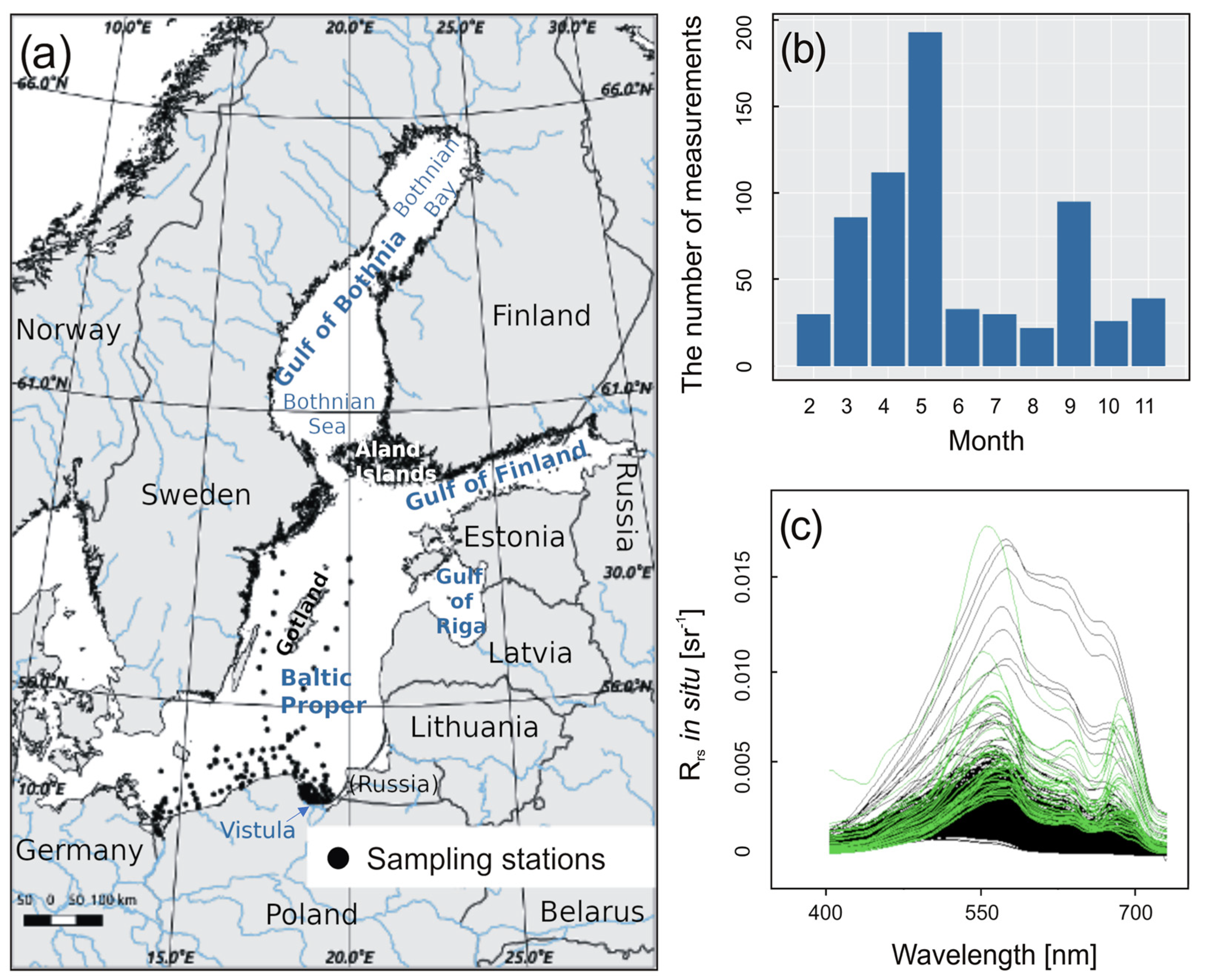
2.1. Study Area

The semi-enclosed location of the Baltic Sea, its intense river runoff, and the relatively low amounts of water it exchanges with the North Sea contribute to its essential ecosystem conditions, with waters that are known to be brackish and which remain under the control of the surrounding lands (Figure 2a). Salinity varies in surface waters from over 20 PSU in the Danish Straits to around 2 PSU in the Bothnian Bay, which fosters the growth of algae taxa that prefer lower salinity. The Baltic Sea’s longitudinal extent of almost 12 degrees, its rugged shoreline, and its position at the mid-latitudes cause additional large seasonal variability and contrasts between its sub-basins [29]. Moreover, the southern regions are more densely populated and cover larger agriculturally used lands, which affect the water properties via river runoff [30]. Of the 28 major rivers that cover 80% of the drainage area, 12 are eutrophic, introducing high nitrogen and phosphorus loads, which generally enter the Baltic Proper or the Gulf of Finland. Most of the remaining rivers discharge in the Bothnian Sea or the Bothnian Bay and provide more silicates [31].

The nutrient resupply process that occurs during winter favors spring blooms, dominated by diatoms and dinoflagellates. After the depletion of nitrogen, diazotrophic cyanobacteria gain a competitive advantage over the other phytoplankton groups, and summer blooms in the Baltic Sea are usually dominated by one of the two main taxa of filamentous cyanobacteria, Aphanizomenon flos-aquae or Nodularia spumigena, often accompanied by Dolichospermum sp. [32]. They thrive until the phosphorus limit is reached [33] unless intense vertical mixing disperses cyanobacteria colonies. The rough sea may cause the temporary disappearance of blooms, which is often the main reason for the difference between the total bloom duration and the effective number of days with bloom observations [34].

2.2. In Situ Measurements

To assess the potential use of the CI in the Baltic Sea, we used a database consisting of 599 data sets collected during cruises onboard the r/v Oceanograf 2 in the years 2012 and 2013, as well as the r/v Oceania and a motorboat, Sonda II, in the years 2016–2018 (Figure 2a). At all stations, the remote sensing reflectance spectra (R_rs) were measured and the water samples were collected for further laboratory analyses of phycocyanin (PC), chlorophyll a (Chl a), and chlorophyll b (Chl b) concentrations to determine the efficiency of the distinction of cyanobacteria from the other phytoplankton groups. Measurements were performed from February until November, omitting December and January due to challenging weather conditions. There was a slightly increased proportion of spring measurements (Figure 2b). However, spring blooms occur in the Baltic Sea around April–May, so a good representation of this part of the year ensures a reliable estimation of efficiency in distinguishing between spring and summer blooms.

Water samples for the estimation of pigment concentrations were collected using Niskin bottles near the surface and passed through Whatman 25 mm GF/F filters under low vacuum (GE Healthcare, Little Chalfont, UK). Filter pads were immediately frozen in liquid nitrogen and transported to the laboratory.

2.2.1. Pigment Concentrations

Chl a and Chl b concentrations were determined using reversed-phase high-performance liquid chromatography (RP-HPLC) according to the method proposed by Stoń and Kosakowska (2002, 2005) [35,36]. PC concentrations were determined on the basis of spectrofluorometric measurements of prepared extracts following the method proposed by Sobiechowska-Sasim et al. (2014) [37].

2.2.2. In Situ Remote Sensing Reflectance

In situ remote sensing reflectance R_rs(λ) spectra were determined using measurements of RAMSES TriOS hyperspectral radiometers (ACC-VIS and MRC) that recorded radiation in 194 spectral bands in the 350 nm–900 nm range with a 3.3 nm step (Figure 2c). The downwelling irradiance above the surface E_s(λ) from the upper sphere was measured using an ACC-VIS radiometer equipped with a cosine collector mounted on the ship’s deck. The upwelling radiation L_u(λ,0⁻) just below the sea surface was recorded using an MRC radiometer mounted on a floating frame and ended with a special tube of 1.6 cm diameter containing the main optical path designed to minimize the self-shading effect [38,39]. Field measurements were collected following the widely accepted NASA protocols, with particular caution taken to avoid ship shadow [40]. R_rs(λ) values were determined as a ratio of the upwelling radiance just above the sea surface L_w(λ), which was derived from the L_u(λ,0⁻) by estimating the propagation of radiation through the water–air interface using the standard 0.543 coefficient, and the E_s(λ) [40,41]. In situ R_rs(λ) spectra were integrated within the satellite bands, taking into account spectral response functions respectively [42].

2.3. Satellite Data

Data from two satellite radiometers, the Ocean and Land Color Instrument (OLCI) and the Moderate-Resolution Imaging Spectroradiometer (MODIS), were used in this study, as those are the most widely used contemporary ocean color sensors and they have been successfully used to derive CI information before [11,26]. To obtain a long homogeneous time series of data to study trends in cyanobacterial blooms in the Baltic Sea, we used MODIS AQUA data registered in 2002–2018. They were downloaded from the NASA Ocean Color portal at Level-0, preprocessed to Level-1, and corrected for the Rayleigh scattering effect using SeaDAS (v. 6.4) software. The final products were MODIS-derived data with a spatial resolution of 1 km, covering the entire Baltic Sea area in the years 2002–2018. However, to minimize adjacent effects and possible bottom reflections, coastal areas shallower than 10 m were excluded from further analyses.

For the comparison between the MODIS and the OLCI sensors (see Section 2.4 and Section 3.1), the OLCI maps (from Sentinel-3A and -3B) registered on 10 May, 14 June, 5 July, 23 July, and 26 August 2018, less than 3 h from the MODIS overpasses, which is a typical time-window for validation purposes [43], were downloaded from the data portal of the European Organisation for the Exploitation of Meteorological Satellites (EUMETSAT, https://data.eumetsat.int/product/EO:EUM:DAT:0409#, accessed on 5 February 2019) at Level-1B and corrected for the Rayleigh scattering effect using SNAP software (v.6.0). Instead of using cloud flags, which are typically produced in the full atmospheric correction process, all pixels from the OLCI maps where the reflectance in the band centered at 940 nm exceeded 0.01 were excluded since even in highly turbid waters or land areas, values in that band were close to zero. Such an approach eliminated land and roughly determined most cloud-contaminated areas sufficiently for the CI index analysis, as shown the example in Figure 3b, and was thus less sensitive to cloud influence than a typical R_rs-based algorithm [44].

2.4. Cyanobacteria Index

CI expresses the relative depth of the local minimum of the reflectance curve caused by the presence of a cyanobacteria bloom (near 680 nm) in relation to the baseline determined by the reflectance measured for wavelengths beyond the valley, and it can be calculated with the following spectral shape (SS) equation:

$$SS\left({\lambda }_0\right)=R\left({\lambda }_0\right)-R\left({\lambda }^{-}\right)-\left\{R\left({\lambda }^{+}\right)-R\left({\lambda }^{-}\right)\right\}\frac{{\lambda }_0-{\lambda }^{-}}{{\lambda }^{+}-{\lambda }^{-}}$$

(1)

where R is reflectance; λ₀ is the central band; and λ⁻ and λ⁺ are the closest bands with shorter and longer wavelengths, respectively, than the central band (λ₀). Considering the differences in the spectral bands between the satellite sensors, the wavelengths used to compute CI were [26,44]:

$$C{I}_{OLCI}=\left(-1\right)\cdot SS\left(681\right)=\left(-1\right)\cdot \left[R_{RC}\left(681\right)-R_{RC}\left(665\right)-\left\{R_{RC}\left(709\right)-R_{RC}\left(665\right)\right\}\frac{681-665}{709-665}\right]$$

(2)

$$C{I}_{MODIS}=\left(-1\right)\cdot SS\left(678\right)=\left(-1\right)\cdot \left[R_{RC}\left(678\right)-R_{RC}\left(667\right)-\left\{R_{RC}\left(748\right)-R_{RC}\left(667\right)\right\}\frac{678-667}{748-667}\right]$$

(3)

where R_RC is the Rayleigh-corrected top-of-atmosphere reflectance.

2.5. Statistical Analyses

The relationship between the MODIS-derived and the OLCI-derived CI values was assessed using the correlation coefficient, the root mean squared error (RMSE), bias, the mean absolute error (MAE), and the mean absolute percentage error (MAPE) [45]. Consequently, we used boxplots that depicted the 1st to 3rd quartiles with a median value in the center and whiskers spanning from −1.5 to +1.5 of the interquartile range (IQR).

Compliance between the data from each of the two satellite sensors was tested using a confusion matrix that determined classification efficiency (the confusionMatrix function implemented in R as part of the caret library v.27.05.2018 [46]). Based on the matrix, Cohen’s kappa value (κ) was determined, which is a common classification assessment metric for evaluating the agreement between two categorical subsets [47]. For the comparison of the sensors presented below (Section 3.1), we adopted cyanobacteria blooms identified in the OLCI images as a reference due to the higher spectral resolution of the OLCI sensor.

3. Results

3.1. CI Comparison for the Two Satellite Sensors

Firstly, the resulting CI_MODIS maps were compared with the CI_OLCI maps since the distribution of the spectral bands varied for the two satellite sensors. Due to computer power constraints, a representative subset was manually selected, consisting of the best cloud-free images acquired within the analyzed blooming season, between June and August, along with evident near-surface bloom images, to obtain a bloom-class area of a statistically robust size. Additionally, a map registered in May was included because at this time of the year, pine pollen grains accumulate on the Baltic Sea surface [48], and these were potentially the largest source of errors. As a result, the images registered on 10 May, 14 June, 5 July, 26 July, and 26 August 2018 were used for comparisons. Images were converted to the same projection and collocated. Based on the matching valid water pixels, the following relationship between CI values acquired from OLCI and MODIS was determined:

CI_OLCI = 0.00058 + 1.83140 · CI_MODIS,

(4)

The bias for the final regression (Equation (4)) was 2·10⁻⁹, and the MAPE was 2.78%. The relationship was used to determine the CI_MODIS value indicating the presence of a bloom. The CI_OLCI threshold was adopted at −0.00001 after Wynne et al. (2010) [44] (not exactly zero due to numerical issues), and the threshold for the CI_MODIS was retrieved from the regression equation (Equation (4)) and estimated at −0.00032. To assess the compatibility between the resulting MODIS and OLCI maps, the results of the bloom area estimations from both sensors were compared using the confusion matrix and κ (

Table 1. Confusion matrix presenting comparisons between cyanobacteria bloom areas derived from OLCI and MODIS data, where class 1 indicates the presence of a bloom and class 0 indicates the absence of a bloom.

		Number of OLCI Pixels
		Class 0 (No Bloom)	Class 1 (Bloom)	Sum
Number of MODIS pixels	Class 0 (no bloom)	1,368,696	22,976	1,391,672
	Class 1 (bloom)	27,113	62,439	89,552
	Total	1,395,809	85,415	κ = 0.70

). The κ metric ranges between zero and one, where zero indicates a lack of agreement, and one indicates identity. Based on 1,481,224 pixels (including only valid sea water pixels), we obtained 96% compliance with a κ value of 0.7.

Additionally, the Rayleigh-corrected reflectance spectra derived from the OLCI (Figure 3a) and MODIS (Figure 3b) sensors were compared in the 600 nm–750 nm range. Several locations during a cyanobacteria bloom on 25 July 2018 were selected manually within the bloom (1–9) and in its vicinity (10–12) (Figure 3c,d). At the stations that appeared bright green in the true color images (1–9), CI index values were positive, with an evident trough for both sensors. At control stations 10–12, the CI index values were negative, including the cloud-covered station 10 in the MODIS AQUA image (Figure 3d), and were classified as non-bloom areas, suggesting lower cell abundances or the presence of cells deeper in the water column.

3.2. Bloom Identification Efficiency

The classification of the presence of cyanobacteria blooms based on the CI calculated at the locations of in situ stations (Figure 2a) was compared to the classifications based on PC and Chl a concentrations. Following the WHO recommendations, stations with Chl a concentrations above 10 mg m⁻³ were identified as areas affected by blooms [9]. The Chl a threshold indicated that 69 stations were locations of blooms, whereas using CI, 25 stations were classified as cyanobacteria bloom areas (Figure 4). At several stations where Chl a exceeded 10 mg m⁻³, PC was lower than 0.1 mg m⁻³. In general, high values of Chl a overlapped a wide range of PC values (Figure 4). CI indicated only stations with relatively high PC values, over 2 mg m⁻³. However, there were two cases where the PC value was higher than 2 mg m⁻³, but CI did not recognize it as a bloom (Figure 4).

One of the two stations with PC values above 10 mg m⁻³, which was not classified as a bloom, was located within the plume of the Vistula River. Vistula plume waters were determined to have a salinity level at least 25% lower than that observed across Gdansk Bay. Nonetheless, the scatterplot of PC versus CI generally showed a clear relationship between PC values and positive CI values that indicated the presence of a bloom (Figure 5a). The correlation coefficient between PC and CI was 0.83 at the stations where PC exceeded 2 mg m⁻³, except for the plume areas. The PC to Chl a ratio was one order of magnitude higher (based on the Mann–Whitney–Wilcoxon test, p < 0.001) within the bloom areas compared to non-bloom areas classified with CI (Figure 5b).

The few stations which were not classified as blooms by CI even though the PC value was higher than 2 mg m⁻³ (Figure 5a) were characterized by a high Chl b to Chl a ratio, suggesting the occurrence of chlorophytes, charophytes, or euglenophytes [49]. Figure 6 shows a clear division into two subsets. One, which was classified as bloom areas, mainly consisted of samples where the Chl b to Chl a ratio remained low, typically below 0.05, whereas within the other class, the Chl b to Chl a ratio reached higher levels, suggesting a varying phytoplankton composition and a dominant taxon other than cyanobacteria (Figure 6).

3.3. Spatial and Temporal Changes of the Cyanobacteria Blooms in the Baltic Sea

The MODIS satellite data from the years 2002–2018 were used to calculate the CI and derive maps of areas covered by cyanobacterial blooms using the threshold mentioned above (in Section 3.1). Finally, for each pixel, the number of days with the presence of cyanobacteria blooms was calculated (Figure 7). The results did not show any long-term change in the maximum bloom area, but the area may have been affected by the presence of cloud. Blooms were somewhat scattered in space, with high year-to-year variability. Only in the northern part of the Baltic proper were cyanobacteria blooms observed almost every year. Blooms persisted for the longest time in the Gulf of Finland, in the summer of 2002. Intense blooms were also noted in 2005, when cyanobacteria thrived at the western coasts of Gotland, and in 2014, when they were focused between the Finnish Coast and the Aland Islands. Until 2018, they were observed there for a notably shorter time. It is worth noting that in the first years, from 2002 to 2004, cyanobacteria blooms did not occur in the Bothnian Sea, whereas since 2005 they have been observed yearly (Figure 7).

Neither the time series of the first day nor of the last day of cyanobacteria blooms showed any significant trends (Figure 8a). Only when we inspected the time between the two, which was called the season of the blooms (after Kahru et al., 2016 [21]), could we see an increasing trend in 2002–2018. This was even more visible when plotting the number of bloom days falling within each month between June and August (Figure 8b). In 2002 and 2003, blooms were observed only in July. After 2004, they lasted until August. Particularly pronounced blooms in August were observed in 2004, 2007, 2012, and 2015. The first year in which a bloom was noted in June was 2005. Early-starting blooms were spotted in 2007, 2009, 2013, and 2016. The longest-lasting, most intense bloom in June was observed in 2009, but after 2007 blooms were observed to have started in June regularly since 2007 and ended in August, demonstrating an evident elongation of the bloom season (Figure 8b). It should be acknowledged that sometimes blooms may disappear in one place but appear in another, so the number of days with the presence of a bloom for the entire Baltic Sea (Figure 8) could be higher than that depicted on the maps (Figure 7).

4. Discussion

Chl-a-based metrics have been widely used in remote sensing to detect phytoplankton blooms. However, recent publications have revealed that in the case of cyanobacteria blooms, estimations based on Chl a may substantially overestimate the sizes of blooms [49]. Due to the specific structure of cyanobacteria cells and their characteristic pigments, the next generation of algorithms has focused on retrieving PC concentrations [17,50], as this is the marker pigment of cyanobacteria [49]. PC values have been shown to correspond better with the abundance of filamentous cyanobacteria, but the performance of algorithms based on the R_rs bands has been hindered by extremely high biomasses observed during blooms concentrated near the sea surface [17], which has resulted in problems with atmospheric correction in the near-infrared region as an indirect effect of a high amount of scattering from the floating colonies [22].

Therefore, the focus of this study was on near-surface aggregations, in which observations across numerous sensors may be affected [4,5,6]. CI was proposed as a complementary method dedicated to extreme bloom events because it does not require full atmospheric correction [26,44], which is still a challenge in the Baltic Sea. It is based on spectral shape analysis, making it less prone to atmospheric correction failures [44]. Additionally, it does not use the band at 620 nm, around the maximum PC absorption level [17], which is specific to cyanobacteria and is promising for their detection [50], but which is missing from the MODIS data. The band at 620 nm was present only in the Medium-Resolution Imaging Spectrometer (MERIS), operating in the years 2002–2012, and the OLCI launched in 2016. Thus, even combining the two data sets would leave a 4-year gap, which is critical in trend analysis.

Our study showed a strong relationship between CI and PC values exceeding 2 mg m⁻³. Although the correlation coefficient between them exceeded 0.8, the number of measurements collected during bloom events was insufficient to develop a reliable model estimating PC, especially considering the good practice of using cross-validation. Thus, our main emphasis was on using the CI as a tool for identifying bloom areas in a dichotomic form that is preferred by the authorities [51]. It was demonstrated that the CI could be successfully applied to detect cyanobacteria-dominated blooms in the Baltic Sea (Figure 5a). CI correctly identified locations where cyanobacteria dominated other phytoplankton communities at a wide range of PC concentrations (Figure 6). The significantly higher PC-to-Chl a ratio within the blooms provided additional evidence of the efficient differentiation achieved using CI (Figure 5b).

One of the main limitations of CI was its insufficient performance in the direct neighborhood of river plumes (Figure 5a). However, in contrast with the methods based on Chl a concentrations, in this case the poor performance was less closely related to sediment loads [52]. River plume areas of the Southern Baltic Sea are highly productive due to the excess nutrients carried by rivers from the land. Therefore, a variety of thriving phytoplankton species that are abundant in Chl a may impact the spectral shape of the reflectance curve and mask the presence of cyanobacteria. Nonetheless, this issue does not decrease the value of the presented method because those are relatively small areas in comparison to the total area of the Baltic Sea. The high κ coefficient observed between bloom areas identified based on MODIS and OLCI data confirms the stability of the method [53]. Even applying strict assessment rules, 0.7 is a satisfactory level that ensures compatibility between both data sets, as well as the repeatability of the results [54].

Apart from algorithms using Chl a, other common algorithms have been developed based on the R_rs values in the red part of the electromagnetic spectrum, relating to the absorption properties of Chl a. Due to its lower penetration depths, the red range is less sensitive to bottom reflection than the green range. It has been a common choice due to the spectral limitations of the first satellite sensors, its similarity to human vision, and the ease of manual inspection using this range. However, algorithms based on the red part of the spectrum have been found to be prone to biases in turbid areas dominated by the strong scattering caused by high loads of suspended sediments [55]. Using one or even two spectral bands makes distinguishing between cyanobacteria and other phytoplankton groups almost impossible. Moreover, such an approach requires additional assumptions considering the typical times of the blooms, usually restricting the analysis period to July–August [55]. The assumption that cyanobacteria blooms occurred only in July and August was valid for years, but recent HELCOM reports proved that we had witnessed a change [56]. Monitoring surveys in 2014 showed that Aphanizomenon flos-aquae was abundant in the Baltic Sea waters already in June [57]. One of the early cyanobacteria bloom events was also confirmed in mid-June of 2021 by the Copernicus service [58]. Using CI enabled us to relax the time restriction but to focus mainly on near-surface accumulations, so the final blooms areas were significantly smaller than the bloom extents reported, e.g., by SMHI [57] and Kahru and Elmgren (2014) [20].

The results based on CI were similar to the independent in situ measurements recorded using the flow-through Ferrybox system along a ferry route from Travemünde (Germany) to Helsinki (Finland) in the summer of 2005 [59]. Keeping in mind the discrepancies between Chl a and PC fluorescence recognized by Groetsch et al. (2014) [59], the PC fluorescence and the bloom’s depth classes were selected for comparison (Figure 9d,e) with the three metrics calculated using MODIS data, including the fluorescence line height (FLH) [10], the floating algae index [60], and the CI values (Figure 9a–c respectively). Even though the FLH may present compromised quality in high-CDOM waters such as the Baltic Sea [61,62], the values should have been positive in the regions of high primary productivity (Figure 9a). Along the transect, FLH values above zero appeared only in a few cases of mixed and stratified blooms (Figure 9e), and around the near-surface cyanobacteria blooms, values were negative (Figure 9a). The FAI index values in the respective areas dropped below zero, but the overall variability probably represented noise (Figure 9b). The FAI index was developed to address a similar problem in atmospheric correction caused by thick scum formations and used short-wave infrared (SWIR) bands [60], but apparently the near-surface cyanobacteria blooms in the Baltic Sea were not pronounced enough to be detected via the FAI index. Only cyanobacteria blooms identified with the CI values corresponded with the near-surface floating cyanobacteria accumulations outlined by Groetsch et al. [59], which indicated that CI could be used to successfully identify the cyanobacteria located in the top layer of the water column in the Baltic Sea (Figure 9c). Since it was effectively used to detect near-surface aggregates, it should be considered an extension of the existing methods for estimating cyanobacteria at lower abundances distributed evenly within water bodies [17]. A combination of both approaches would allow one to obtain a full picture.

Analyses of changes in time and space using satellite data series revealed an increasing trend in terms of the cyanobacteria bloom season length, that is, the time between the first and the last day on which a bloom was observed each year (Figure 8a). Blooms were observed only in July at the beginning of the analyzed period. However, after 2005 they were frequently observed earlier, in June, and in several years they lasted until August (Figure 8b). The nominal number of bloom days did not increase significantly in the years 2002–2018, but the cloud cover might have affected the trend’s significance. The occurrence of prolonged bloom seasons that are not in line with the nominal number of days with blooms imply limiting factors other than temperature. Even though the water temperatures were high enough to foster primary productivity for a longer time every year, other factors could prevent the development of cyanobacteria blooms [21,63,64]. For example, storm waves, intense winds, or cloudiness may cause significant disappearances of blooms [6] and diminish the overall number of days with visible near-surface accumulations, resulting in the absence of increasing trends with regard to bloom area. Unfortunately, the optical sensors used in this study did not allow for a distinction between the lack of information due to the presence of clouds or due to total bloom dispersion caused by strong winds and waves, which may accompany weather conditions that hinder bloom development. Although an increase in the overall length of the vegetative season in the western Baltic Sea was also reported by Wasmund et al. [65], the intensification of the cyanobacteria blooms could not be unequivocally verified. It is possible that there are not one or two driving factors but several, depending on the time scale, since Kahru et al. [56] found that the phosphorus concentration and the extent of hypoxic areas were also significant factors on the inter-annual scale. In contrast, temperature and irradiance appeared critical in relation to year-to-year variability. Another hypothesis considers cyanophages to be a significant factor in regulating cyanobacteria populations [63]. Another possibility is that higher average temperatures created a niche for other types of non-toxic picocyanobacteria to thrive. A recent study by Stoń-Egiert and Ostrowska [33] displayed an increasing trend with regard to zeaxanthin in the Baltic Sea, with zeaxanthin being a common pigment among many cyanobacteria strains, although not in two out of three analyzed here—Nodularia sp. and Dolichospermum sp. [16].

Nonetheless, this study confirmed the northward progression of cyanobacteria and their regular appearance in the Bothnian Sea in the last few years. This finding is consistent with a study by Kahru et al. [20], in which blooms in that area in the 1980s and 1990s were found to be sporadic, and with previous predictions that the Bothnian Sea would become more nitrogen-limited due to inflows of additional phosphorus loads from the Baltic proper [66]. Diazotrophic cyanobacteria thrive in a nitrogen-limited environment, and even in the Baltic proper, and they outcompete other taxa when nitrogen is depleted. The first in situ records of an increasing cyanobacteria biomass in the Bothnian Sea during summer have already been reported to HELCOM [67]. Unfortunately, we were not able to make determinations regarding differences between species using satellite images, but in situ collected data presented elsewhere showed clearly that the biomasses of Aphanizomenon flos-aquae and Dolichospermum sp. had increased in the northern Bothnian Sea [18]. Therefore, further monitoring will be crucial in the coming years, and only by combining in situ and satellite measurements will we be able to provide a complete picture of the changes occurring in the marine environment.

5. Conclusions

Our study showed that the cyanobacteria index was an efficient method to identify cyanobacteria blooms in the Baltic Sea, and proved that it could be used to successfully distinguish cyanobacteria-dominated events from those dominated by any other phytoplankton group. Comparisons with in situ data confirmed that measures taking into account specific cyanobacteria absorption and fluorescence traits, such as the CI, performed better than the most commonly used methods based on the Chl a concentration, fluorescence, or reflectance thresholds. CI was successfully used to identify extreme situations in which cyanobacteria accumulated near the surface and could be used as a complementary method to the algorithms designed previously for detecting lower abundances of cyanobacteria scattered in the water column. Maps of cyanobacteria bloom time-series derived from satellite data using CI showed a significant elongation of the bloom season, defined as the time between the first and the last observation of a bloom. However, the intensification of cyanobacteria blooms was unclear due to cloud-cover restrictions, which is the main concern in the monitoring of cyanobacterial blooms from satellite images with CI, and addressing the problem of persistent cloud cover should be the next step in this area of study.

References

1. Mazur-Marzec, H.; Pliński, M. Do toxic cyanobacteria blooms pose a threat to the Baltic ecosystem? Oceanologia 2009, 51, 293–319. [Google Scholar] [CrossRef] [Green Version]
2. Reinart, A.; Kutser, T. Comparison of different satellite sensors in detecting cyanobacterial bloom events in the Baltic Sea. Remote Sens. Environ. 2006, 102, 74–85. [Google Scholar] [CrossRef]
3. Ploug, H. Cyanobacterial surface blooms formed by Aphanizomenon sp. and Nodularia spumigena in the Baltic Sea: Small-scale fluxes, pH, and oxygen microenvironments. Limnol. Oceanogr. 2008, 53, 914–921. [Google Scholar] [CrossRef] [Green Version]
4. Bresciani, M.; Adamo, M.; de Carolis, G.; Matta, E.; Pasquariello, G.; Vaičiūtė, D.; Giardino, C. Monitoring blooms and surface accumulation of cyanobacteria in the Curonian Lagoon by combining MERIS and ASAR data. Remote Sens. Environ. 2014, 146, 124–135. [Google Scholar] [CrossRef]
5. Kahru, M.; Leppänen, J.-M.; Rud, O. Cyanobacterial blooms cause heating of the sea surface. Mar. Ecol. Prog. Ser. 1993, 101, 1–7. [Google Scholar] [CrossRef]
6. Kanoshina, I.; Lips, U.; Leppänen, J.-M. The influence of weather conditions (temperature and wind) on cyanobacterial bloom development in the Gulf of Finland (Baltic Sea). Harmful Algae 2003, 2, 29–41. [Google Scholar] [CrossRef]
7. Nebaeus, M. Algal water-blooms under ice-cover. Verh. Internat. Verein. Limnol. 1971, 22, 719–724. [Google Scholar] [CrossRef]
8. Steidinger, K.A.; Garccés, E. Importance of Life Cycles in the Ecology of Harmful Microalgae. In Ecology of Harmful Algae; Granéli, E., Turner, J.T., Eds.; Springer: Berlin/Heidelberg, Germany, 2006; ISBN 978-3-540-32210-8. [Google Scholar]
9. Hollister, J.W.; Kreakie, B.J. Associations between chlorophyll a and various microcystin health advisory concentrations. F1000Research 2016, 5, 151. [Google Scholar] [CrossRef] [Green Version]
10. Behrenfeld, M.J.; Westberry, T.K.; Boss, E.S.; O’Malley, R.T.; Siegel, D.A.; Wiggert, J.D.; Franz, B.A.; McClain, C.R.; Feldman, G.C.; Doney, S.C.; et al. Satellite-detected fluorescence reveals global physiology of ocean phytoplankton. Biogeosci. Discuss. 2008, 5, 4235–4270. [Google Scholar] [CrossRef] [Green Version]
11. Naghdi, K.; Moradi, M.; Kabiri, K.; Rahimzadegan, M. The effects of cyanobacterial blooms on MODIS-L2 data products in the southern Caspian Sea. Oceanologia 2018, 60, 367–377. [Google Scholar] [CrossRef]
12. Govindjee, G. Chlorophyll a Fluorescence: A Bit of Basics and History. In Chlorophyll Fluorescence: A Signature of Photosynthesis; Papageorgiou, G.C., Govindjee, G., Eds.; Springer: Dordrecht, The Netherlands, 2004; ISBN 978-1-4020-3218-9. [Google Scholar]
13. Dall’Olmo, G.; Gitelson, A.A. Effect of bio-optical parameter variability and uncertainties in reflectance measurements on the remote estimation of chlorophyll-a concentration in turbid productive waters: Modeling results. Appl. Opt. 2006, 45, 3577–3598. [Google Scholar] [CrossRef] [PubMed] [Green Version]
14. Bailey, S.; Grossman, A. Photoprotection in Cyanobacteria: Regulation of Light Harvesting. Photochem. Photobiol. 2008, 84, 1410–1420. [Google Scholar] [CrossRef] [PubMed]
15. Roy, S.; Llewellyn, C.A.; Egeland, E.S.; Johnsen, G. Phytoplankton Pigments: Characterization, Chemotaxonomy and Applications in Oceanography; Cambridge University Press: Cambridge, UK, 2011; 890p, ISBN 978-1-107-00066-7. [Google Scholar]
16. Wojtasiewicz, B.; Stoń-Egiert, J. Bio-optical characterization of selected cyanobacteria strains present in marine and freshwater ecosystems. J. Appl. Phycol. 2016, 28, 2299–2314. [Google Scholar] [CrossRef] [PubMed] [Green Version]
17. Woźniak, M.; Bradtke, K.; Darecki, M.; Krężel, A. Empirical Model for Phycocyanin Concentration Estimation as an Indicator of Cyanobacterial Bloom in the Optically Complex Coastal Waters of the Baltic Sea. Remote Sens. 2016, 8, 212. [Google Scholar] [CrossRef] [Green Version]
18. Olofsson, M.; Klawonn, I.; Karlson, B. Nitrogen fixation estimates for the Baltic Sea indicate high rates for the previously overlooked Bothnian Sea. Ambio 2021, 50, 203–214. [Google Scholar] [CrossRef] [Green Version]
19. Rantajärvi, E. Alg@line in 2003: 10 Years of Innovative Plankton Monitoring and Research and Operational Information Service in the Baltic Sea; MERI—Report Series of the Finnish Institute of Marine Research; Merentutkimuslaitos: Helsinki, Finland, 2003; p. 48. ISBN 951-53-2507-2. [Google Scholar]
20. Kahru, M.; Elmgren, R. Multidecadal time series of satellite-detected accumulations of cyanobacteria in the Baltic Sea. Biogeosciences 2014, 11, 3619–3633. [Google Scholar] [CrossRef] [Green Version]
21. Kahru, M.; Elmgren, R.; Savchuk, O.P. Changing seasonality of the Baltic Sea. Biogeosciences 2016, 13, 1009–1018. [Google Scholar] [CrossRef] [Green Version]
22. Kutser, T. Passive optical remote sensing of cyanobacteria and other intense phytoplankton blooms in coastal and inland waters. Int. J. Remote Sens. 2009, 30, 4401–4425. [Google Scholar] [CrossRef]
23. Philpot, W.D. The Derivative Ratio Algorithm: Avoiding Atmospheric Effects in Remote Sensing. IEEE Trans. Geosci. Remote Sens. 1991, 29, 350–357. [Google Scholar] [CrossRef]
24. Schowengerdt, R.A. Remote Sensing: Models and Methods for Image Processing; Elsevier: Enschede, The Netherlands, 2006; ISBN 9780080480589. [Google Scholar]
25. Stumpf, R.P.; Werdell, P.J. Adjustment of ocean color sensor calibration through multi-band statistics. Opt. Express 2010, 18, 401–412. [Google Scholar] [CrossRef] [Green Version]
26. Wynne, T.T.; Stumpf, R.P.; Briggs, T.O. Comparing MODIS and MERIS spectral shapes for cyanobacterial bloom detection. Int. J. Remote Sens. 2013, 34, 6668–6678. [Google Scholar] [CrossRef]
27. Stumpf, R.P.; Davis, T.W.; Wynne, T.T.; Graham, J.L.; Loftin, K.A.; Johengen, T.H.; Gossiaux, D.; Palladino, D.; Burtner, A. Challenges for mapping cyanotoxin patterns from remote sensing of cyanobacteria. Harmful Algae 2016, 54, 160–173. [Google Scholar] [CrossRef] [PubMed]
28. Mishra, S.; Stumpf, R.P.; Schaeffer, B.A.; Werdell, J.P.; Loftin, K.A.; Meredith, A. Measurement of Cyanobacterial Bloom Magnitude using Satellite Remote Sensing. Sci. Rep. 2019, 9, 18310. [Google Scholar] [CrossRef] [Green Version]
29. Leppäranta, M.; Myrberg, K. Physical Oceanography of the Baltic Sea; Springer Science & Business Media: Berlin, Germany, 2009; ISBN 978-3-540-79702-9. [Google Scholar]
30. Andrén, E.; Snoeijs-Leijonmalm, P. Why is the Baltic Sea so special to live in? In Biological Oceanography of the Baltic Sea; Snoeijs-Leijonmalm, P., Schubert, H., Radziejewska, T., Eds.; Springer: Dordrecht, The Netherlands, 2017; ISBN 978-94-007-0667-5. [Google Scholar]
31. Pastuszak, M.; Kowalkowski, T.; Kopiński, J.; Doroszewski, A.; Jurga, B.; Buszewski, B. Long-term changes in nitrogen and phosphorus emission into the Vistula and Oder catchments (Poland)—Modeling (MONERIS) studies. Environ. Sci. Pol. Res. 2018, 25, 29734–29751. [Google Scholar] [CrossRef] [PubMed] [Green Version]
32. Mazur-Marzec, H.; Kężel, A.; Kobos, J.; Pliński, M. Toxic Nodularia spumigena blooms in the coastal waters of the Gulf of Gdańsk: A ten-year survey. Oceanologia 2006, 48, 255–273. [Google Scholar]
33. Stoń-Egiert, J.; Ostrowska, M. Long-term changes in phytoplankton pigment contents in the Baltic Sea: Trends and spatial variability during 20 years of investigations. Cont. Shelf Res. 2022, 236, 104666. [Google Scholar] [CrossRef]
34. Paerl, H.W.; Fulton, R.S. Ecology of Harmful Cyanobacteria. In Ecology of Harmful Algae; Granéli, E., Turner, J.T., Eds.; Springer: Berlin/Heidelberg, Germany, 2006; ISBN 978-3-540-32210-8. [Google Scholar]
35. Stoń, J.; Kosakowska, A. Phytoplankton pigments designation–an application of RP-HPLC in qualitative and quantitative analysis. J. Appl. Phycol. 2002, 14, 205–210. [Google Scholar] [CrossRef]
36. Stoń-Egiert, J.; Kosakowska, A. RP-HPLC determination of phytoplankton pigments—Comparison of calibration results for two columns. Mar. Biol. 2005, 147, 251–260. [Google Scholar] [CrossRef]
37. Sobiechowska-Sasim, M.; Stoń-Egiert, J.; Kosakowska, A. Quantitative analysis of extracted phycobilin pigments in cyanobacteria—An assessment of spectrophotometric and spectrofluorometric methods. J. Appl. Phycol. 2014, 26, 2065–2074. [Google Scholar] [CrossRef] [Green Version]
38. Gordon, H.R.; Ding, K. Self-shading of in-water optical instruments. Limnol. Oceanogr. 1992, 37, 491–500. [Google Scholar] [CrossRef]
39. Zibordi, G.; Ferrari, G.M. Instrument self-shading in underwater optical measurements: Experimental data. Appl. Opt. 1995, 34, 2750–2754. [Google Scholar] [CrossRef]
40. Mueller, J.L.; Fargion, G.S.; McClain, C.R. Ocean Optics Protocols for Satellite Ocean Color Sensor Validation—Revision 4, Volume III: Radiometric Measurements and Data Analysis Protocols; NASA Technical Report; NASA/TM-2003-21621/Rev-Vol III; NASA: Greenbelt, MD, USA, 2003.
41. Austin, R.W. Optical aspects of oceanography. In The Remote Sensing of Spectral Radiance from below the Ocean Surface; Jerlov, N.G., Nielsen, E.S., Eds.; Academic Press: New York, NY, USA, 1974; pp. 317–344. [Google Scholar]
42. Pelloquin, C.; Nieke, J. Sentinel-3 OLCI and SLSTR Simulated Spectral Response Functions S3-TN-ESA-PL-316. In Proceedings of the Sentinel-3 OLCI/SLSTR and MERIS/(A)ATSR, 711(2), ESA Communications, Noordwijk, The Netherlands, 15–19 October 2012. [Google Scholar]
43. Bailey, S.W.; Werdell, P.J. A multi-sensor approach for the on-orbit validation of ocean color satellite data products. Remote Sens. Environ. 2006, 102, 12–23. [Google Scholar] [CrossRef]
44. Wynne, T.T.; Stumpf, R.P.; Tomlinson, M.C.; Dyble, J. Characterizing a cyanobacterial bloom in western Lake Erie using satellite imagery and meteorological data. Limnol. Oceanogr. 2010, 55, 2025–2036. [Google Scholar] [CrossRef] [Green Version]
45. Chai, T.; Draxler, R.R. Root mean square error (RMSE) or mean absolute error (MAE)?—Arguments against avoiding RMSE in the literature. Geosci. Model Dev. 2014, 7, 1247–1250. [Google Scholar] [CrossRef] [Green Version]
46. Kuhn, M.; Wing, J.; Weston, S.; Williams, A.; Keefer, C.; Engelhardt, A.; Cooper, T.; Mayer, Z.; Kenkel, B.; R Core Team; et al. Caret: Classification and Regression Training. R package version 6.0-84. 2020. Available online: https://cran.r-project.org/web/packages/caret/index.html (accessed on 17 October 2022).
47. Cohen, J. A coefficient of agreement for nominal scales. Educ. Psychol. Meas. 1960, 20, 37–46. [Google Scholar] [CrossRef]
48. Pawlik, M.; Ficek, D. Pine pollen grains in coastal waters of the Baltic Sea. Oceanol. Hydrobiol. Stud. 2016, 45, 35–41. [Google Scholar] [CrossRef]
49. Schlüter, L.; Lauridsen, T.L.; Krogh, G.; Jørgensen, T. Identification and quantification of phytoplankton groups in lakes using new pigment ratios—A comparison between pigment analysis by HPLC and microscopy. Freshw. Biol. 2006, 51, 1474–1485. [Google Scholar] [CrossRef]
50. Qi, L.; Hu, C.; Duan, H.; Cannizzaro, J.; Ma, R. A novel MERIS algorithm to derive cyanobacterial phycocyanin pigment concentrations in a eutrophic lake: Theoretical basis and practical considerations. Remote Sens. Environ. 2014, 154, 298–317. [Google Scholar] [CrossRef]
51. Attila, S.; Fleming-Lehtinen, V.; Attila, J.; Junttila, S.; Alasalmi, H.; Hällfors, H.; Kervinen, M.; Koponen, S. A novel earth observation based ecological indicator for cyanobacterial blooms. Int. J. Appl. Earth Obs. Geoinf. 2018, 64, 145–155. [Google Scholar] [CrossRef]
52. Gower, J.; King, S. On the importance of a band at 709 nm. In Proceedings of the 2nd MERIS (A)ATSR User Workshop, Frascati, Italy, 22–26 September 2008. [Google Scholar]
53. Landis, J.R.; Koch, G.G. The measurement of observer agreement for categorical data. Biometrics 1977, 33, 159–174. [Google Scholar] [CrossRef] [Green Version]
54. McHugh, M.L. Interrater reliability: The kappa statistic. Biochem. Med. 2012, 22, 276–282. [Google Scholar] [CrossRef]
55. Kahru, M.; Savchuk, O.P.; Elmgren, R. Satellite measurements of cyanobacterial bloom frequency in the Baltic Sea: Interannual and spatial variability. Mar. Ecol. Prog. Ser. 2007, 343, 15–23. [Google Scholar] [CrossRef]
56. Kahru, M.; Elmgren, R.; Kaiser, J.; Wasmund, N.; Savchuk, O. Cyanobacterial Blooms in the Baltic Sea: Correlations with Environmental Factors. Harmful Algae 2020, 92, 101739. [Google Scholar] [CrossRef]
57. Öberg, J. Cyanobacteria blooms in the Baltic Sea. HELCOM Baltic Sea Environment Fact Sheet 2014. Available online: https://helcom.fi/baltic-sea-trends/environment-fact-sheets/eutrophication/cyanobacteria-biomass/ (accessed on 30 December 2021).
58. Copernicus. Early Algal Bloom in the Baltic Sea. Image of the Day Series, EU, Copernicus Senitnel-2 Imagery. 2021. Available online: https://www.copernicus.eu/en/media/image-day-gallery/early-algal-bloom-baltic-sea (accessed on 30 December 2021).
59. Groetsch, P.M.M.; Simis, S.G.H.; Eleveld, M.A.; Peters, S.W.M. Cyanobacterial bloom detection based on coherence between ferrybox observations. J. Mar. Syst. 2014, 140, 50–58. [Google Scholar] [CrossRef] [Green Version]
60. Hu, C. A novel ocean color index to detect floating algae in the global oceans. Remote Sens. Environ. 2009, 113, 2118–2129. [Google Scholar] [CrossRef]
61. Gilerson, A.; Zhou, J.; Hlaing, S.; Ioannou, I.; Gross, B.; Moshary, F.; Ahmed, S. Fluorescence component in the reflectance spectra from coastal waters. II. Performance of retrieval algorithms. Opt. Express 2008, 16, 2446–2460. [Google Scholar] [CrossRef] [PubMed]
62. Kowalczuk, P.; Darecki, M.; Zabłocka, M.; Górecka, I. Validation of empirical and semi-analytical remote sensing algorithms for estimating absorption by Coloured Dissolved Organic Matter in the Baltic Sea from SeaWiFS and MODIS imagery. Oceanologia 2010, 52, 171–196. [Google Scholar] [CrossRef] [Green Version]
63. Yoshida, M.; Yoshida, T.; Kashima, A.; Takashima, Y.; Hosoda, N.; Nagasaki, K.; Hiroishi, S. Ecological Dynamics of the Toxic Bloom-Forming Cyanobacterium Microcystis aeruginosa and Its Cyanophages in Freshwater. Appl. Environ. Microbiol. 2008, 74, 3269–3273. [Google Scholar] [CrossRef] [Green Version]
64. Śliwińska-Wilczewska, S.; Cieszyńska, A.; Konik, M.; Maculewicz, J.; Latała, A. Environmental drivers of bloom-forming cyanobacteria in the Baltic Sea: Effects of salinity, temperature, and irradiance. Estuar. Coast. Shelf Sci. 2019, 219, 139–150. [Google Scholar] [CrossRef]
65. Wasmund, N.; Nausch, G.; Gerth, M.; Busch, S.; Burmeister, C.; Hansen, R.; Sadkowiak, B. Extension of the growing season of phytoplankton in the western Baltic Sea in response to climate change. Mar. Ecol. Prog. Ser. 2019, 622, 1–16. [Google Scholar] [CrossRef] [Green Version]
66. Rolff, C.; Elfwing, T. Increasing nitrogen limitation in the Bothnian Sea, potentially caused by inflow of phosphate-rich water from the Baltic Proper. Ambio 2005, 44, 601–611. [Google Scholar] [CrossRef] [PubMed] [Green Version]
67. Kownacka, J.; Busch, S.; Göbel, J.; Gromisz, S.; Hällfors, H.; Höglander, H.; Huseby, S.; Jaanus, A.; Jakobsen, H.H.; Johansen, M.; et al. Cyanobacteria biomass 1990–2018. HELCOM Baltic Sea Environment Fact Sheets 2018. Available online: https://helcom.fi/baltic-sea-trends/environment-fact-sheets/eutrophication/cyanobacteria-biomass/ (accessed on 2 September 2020).
Figure 1. True color image of the Baltic Sea obtained from the Moderate-Resolution Imaging Spectroradiometer (MODIS) on the satellite AQUA, recorded on 13 July 2002 (a), and the Normalized fluorescence line height (NFLH) index values overlayed with the flags developed by the NASA Ocean Biology Processing Group (OBPG) to exclude suspicious pixels after the default atmospheric correction (b). LAND indicates the terrestrial area; TURBIDW, turbid water, ATMWARN, suspected results of the atmospheric correction; CHLFAIL + CHLWARN, possible chlorophyll-a derivation failure.
Remotesensing 15 01601 g001
Figure 2. Locations of the in situ measurements (a), their distribution through the year (b), and all measured reflectance spectra used in our analyses with the bloom spectra marked in green (c).
Remotesensing 15 01601 g002
Figure 3. Comparison of the spectral shapes of Rayleigh-corrected reflectance for OLCI (a) and MODIS (b) in the 600 nm–750 nm range, observed in an exemplary cyanobacteria bloom image registered on 25 July 2018 at 08:36 a.m. and 11:05 a.m., respectively. The location of the spectra was marked in the true color OLCI (c) and MODIS (d) images, with the blue pins showing non-bloom (10–12) spectra.
Remotesensing 15 01601 g003
Figure 4. Scatterplot of phycocyanin (PC) concentrations (mg m−3) versus chlorophyll a (Chl a) concentrations (mg m−3) with shaded measurements identified as cyanobacteria bloom locations based on the typical chlorophyll a threshold exceeding 10 mg m−3 (marked with texture), and those identified based on CI, derived from in situ measurements, depicted as red dots.
Remotesensing 15 01601 g004
Figure 5. Relationship between phycocyanin (PC) concentrations (mg m−3) and CI values derived from in situ measured RRS (a) and the distribution of the ratio of phycocyanin to chlorophyll-a concentrations at locations identified as bloom and non-bloom areas based on CI (b). The points representing PC values above 2 mg m−3 and not classified as blooms are designated with a red square. Boxes were stretched between the 1st (Q1) and the 3rd (Q3) quartile, with the median value as a central line and whiskers spanning from −1.5 to +1.5 of the interquartile range (IQR).
Remotesensing 15 01601 g005
Figure 6. Relationship between the chlorophyll b to chlorophyll a ratio (–) and phycocyanin concentration (mg m−3) at the stations where the phycocyanin concentration exceeded 2 mg m−3. Those classified as blooms are marked in green and the others are marked in red (red square in Figure 5a).
Remotesensing 15 01601 g006
Figure 7. Maps presenting the percentages of summer days (June–August) each year between 2002–2018 when cyanobacteria blooms were identified in the MODIS (AQUA) images.
Remotesensing 15 01601 g007
Figure 8. Time series of the first and the last days on which a cyanobacteria bloom was observed, with the length of the time period between them and a trend line marked in gray (season length) (a), as well as the number of days when a cyanobacteria bloom was observed each year, with a distinction between the months (b).
Remotesensing 15 01601 g008
Figure 9. A comparison of time series of the fluorescence line height (FLH) values derived from MODIS data (a), the floating algae index (FAI) (b), the CI (c), bloom type, (d) and relative PC values (e) along the route of the ferry from Travemünde to Helsinki, measured in 2005 (panels d–e reprinted from Groetsch et al. [47]).
Remotesensing 15 01601 g009