Multivariate Calibration of the SWAT Model Using Remotely Sensed Datasets

Abstract

Remotely sensed hydrologic variables, in conjunction with streamflow data, have been increasingly used to conduct multivariable calibration of hydrologic model parameters. Here, we calibrated the Soil and Water Assessment Tool (SWAT) model using different combinations of streamflow and remotely sensed hydrologic variables, including Atmosphere–Land Exchange Inverse (ALEXI) Evapotranspiration (ET), Moderate Resolution Imaging Spectroradiometer (MODIS) ET, and Soil MERGE (SMERGE) soil moisture. The results show that adding remotely sensed ET and soil moisture to the traditionally used streamflow for model calibration can impact the number and values of parameters sensitive to hydrologic modeling, but it does not necessarily improve the model performance. However, using remotely sensed ET or soil moisture data alone led to deterioration in model performance as compared with using streamflow only. In addition, we observed large discrepancies between ALEXI or MODIS ET data and the choice between these two datasets for model calibration can have significant implications for the performance of the SWAT model. The use of different combinations of streamflow, ET, and soil moisture data also resulted in noticeable differences in simulated hydrologic processes, such as runoff, percolation, and groundwater discharge. Finally, we compared the performance of SWAT and the SWAT-Carbon (SWAT-C) model under different multivariate calibration setups, and these two models exhibited pronounced differences in their performance in the validation period. Based on these results, we recommend (1) the assessment of various remotely sensed data (when multiple options available) for model calibration before choosing them for complementing the traditionally used streamflow data and (2) that different model structures be considered in the model calibration process to support robust hydrologic modeling.

1. Introduction

The conventional approach to calibrating hydrologic models often involves using streamflow data from hydrologic gauges to obtain the optimum values of model parameters for improved model performance [1,2]. However, relying solely on streamflow data to constrain hydrologic model performances can result in the poor simulation of other hydrologic components such as evapotranspiration and soil moisture. In addition, streamflow data may not be readily available for a study region and time of interest due to the high cost and the discontinuity of hydrologic gauge operation. Due to these limitations, when a hydrologic model is calibrated against streamflow data available at the watershed outlet, the simulated hydrologic processes (e.g., streamflow, soil moisture, and ET) within the watershed can be subject to large uncertainties [3,4].

Remotely sensed data can provide crucial information about the dynamics of the water budget [5,6,7,8]. As such, the hydrologic calibration process can benefit from the inclusion of remotely sensed soil moisture [9] and ET [10,11] data, in addition to traditionally used streamflow measurements, to capture the spatiotemporal distribution of the water budget components [2,12,13], particularly in arid/semi-arid watersheds with regulated water resources systems, where evapotranspiration (ET) and soil moisture content play an important role in determining groundwater recharge and irrigation water requirements [7,14].

Among the numerous agrohydrologic models, the Soil and Water Assessment Tool (SWAT) [15] is a representative model that has been widely used for watershed management and water quality studies in agricultural watersheds. To improve the reliability of the SWAT simulations in both gauged and ungauged watersheds, satellite-based data products that represent land surface dynamics (such as leaf area index) and water budget components (such as ET and soil moisture) have proven to be useful [16,17,18,19,20,21]. Many studies have used remotely sensed data, and ET [1,2,10,22,23] or soil moisture [16,17,19] in particular, in conjunction with streamflow data to constrain the complex land–vegetation–atmosphere interaction in hydrologic models. These efforts aid in model parameter estimation and help improve model performance in capturing the spatial and temporal distribution of the water budget components cycle.

For example, Parajuli et al. [2] used Moderate Resolution Imaging Spectroradiometer (MODIS) ET to evaluate if calibration using remotely sensed ET in combination with streamflow improves the streamflow simulation. Their findings suggested that multivariable calibration using remotely sensed data improved ET estimation, but the improvement in streamflow estimation was negligible. Rajib et al. [22] found that multivariable calibration of streamflow and MODIS ET allows for the optimization of model biophysical parameters that improve the representation of vegetation dynamics and effectively reproduced both water and energy balance components. Lee et al. [10] used Atmosphere–Land Exchange Inverse (ALEXI) ET in conjunction with streamflow and crop yield for multivariable calibration and demonstrated that the use of multiple constraints during model calibration helps reduce the model predictive uncertainty by minimizing the number of acceptable parameter sets.

Similar findings have been reported when the hydrologic models were calibrated using streamflow and soil moisture. For instance, Choudhary and Athira [16] used streamflow and soil moisture together to calibrate the SWAT model. They found that calibration with streamflow data alone resulted in poor simulation of soil moisture and significantly different ET simulation compared to the calibration with streamflow and soil moisture together. They showed that constraining the simulated soil moisture slightly improved the baseflow simulation but the trade-off between surface runoff and soil moisture did not significantly improve the overall streamflow simulation. Rajib et al. [19] found that calibration with streamflow data alone resulted in considerable uncertainty in soil moisture simulation, while inclusion of root zone soil moisture improved soil moisture simulation, reduced model uncertainty range, and significantly improved streamflow simulation.

Nevertheless, many issues exist with multivariable calibration and constraining the SWAT model with remotely sensed data. First, although the remotely sensed ET datasets are validated with measured data, their accuracy is subject to uncertainties in inputs (to algorithms deriving remotely sensed ET), temporal and spatial scaling, and coverage [24,25,26] that may cause hydrologic models to produce less accurate results for other components of the hydrologic cycle (e.g., soil moisture, baseflow, and groundwater discharge). With the continuous advancement in satellite technology and consistent global monitoring, multiple remotely sensed data products for evapotranspiration and soil moisture are becoming widely available [27,28]. Notably, remotely sensed ET products differ from each other in terms of the algorithms used to derive the ET values and their capability to provide accurate estimates of ET in a region of interest. Second, a multivariable calibration approach can lead to complications due to trade-offs among model responses [29,30]. For example, the model parametrization can cause the predicted variable, e.g., streamflow, to be closer to the measured values at the cost of other components of the hydrologic processes such as ET, soil moisture, and groundwater discharge.

In addition, the structure or configuration of a hydrologic model can influence the model’s performance, calibrated parameter values, and response to different inputs [31,32]. Another strategy increasingly adopted in the SWAT modeling community to improve model performance consists of model modification to replace simplified empirical algorithms with physically based modules/algorithms that better represent physical processes such as plant growth [33], soil organic carbon, nitrogen cycling [34,35], and soil moisture content and temperature [36]. For example, Qi et al. [3] and Wang et al. [37] showed that modification of the SWAT model’s biogeochemical and energy balance algorithms can influence the SWAT model-simulated hydrologic budgets and their responses to climate change.

Given the above knowledge gaps identified based on the literature review, we aim to provide insights into the following scientific questions: (1) Does the use of different remotely sensed ET and soil moisture products in addition to streamflow data help improve the performance of a calibrated hydrologic model? (2) Does the choice of different remotely sensed ET products for model calibration influence model performance? (3) Do variations in model structure influence model performance under multivariate calibration? The remote sensing datasets and hydrologic model are both open-access to the community. The results from this study are expected to help the hydrologic modeling community to better understand the strengths and caveats of using remotely sensed datasets, thereby designing more robust strategies for improving hydrologic modeling.

2. Materials and Methods

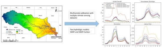
2.1. Study Area

The 6909 km² Little Blue River Watershed (LBRW), located in the Midwest of the USA, spans Nebraska and Kansas (Figure 1). The LBRW is an intensively irrigated agricultural watershed, with agricultural land (69.5%) as the dominant land cover category, followed by pastureland (28.8%) and forest (1.6%). The LBRW is part of the large High Plains Aquifer, where most of the agricultural irrigation is from groundwater. From 1985 to 2015, the annual irrigation water use in the watershed increased from 105 × 10⁶ to 141 × 10⁶ m³ [38]. The watershed receives about 815 mm of rainfall annually with almost 65% of annual rainfall occurring in May–September [39]. The basin is primarily composed of silt loam and silt clay loam soils that have a large water-holding capacity and are relatively impermeable; hence, the groundwater recharge is a small fraction of the annual precipitation [40]. The intensive use of groundwater for irrigation has significantly affected the water quantity in the study area. Moreover, agricultural activities have aggravated the water quality issues in the watershed [41,42]. The hydrologic processes in the LRBW are complex, with substantial surface water and groundwater interaction [42], which is influenced by factors such as surface runoff, infiltration, and evapotranspiration. Given these conditions, water conservation is of utmost importance in the LBRW.

2.2. Hydrologic Models

2.2.1. SWAT Model Description

The SWAT model is a physically based model that simulates hydrologic processes by dividing the watershed into subbasins which are further divided into hydrologic response units (HRU). The HRU represents a unique combination of homogenous land use, soil class, and slope [43]. The surface runoff is simulated using the Natural Resources Conservation Service (NRCS) curve number method, and the flow of water within the soil profile is simulated using a simple tipping bucket approach [43]. This simplified soil moisture model has been widely tested in several studies [44,45]. SWAT simulates the land phase of the hydrologic cycle based on the water balance equation [43]:

$${SW}_t={SW}_o+{\sum }_{i=1}^t(R_{day}-Q_{surf}-E_a-W_{seep}-Q_{gw}),$$

(1)

where SW_t is the soil water content (mm); SW_ο is the initial soil water content (mm); Q_surf is the surface runoff (mm); R_day is the precipitation (mm); E_a is the evapotranspiration (mm); W_seep is the percolation (mm) from the soil profile; Q_gw is the return flow (mm); and t is the time (days).

Evapotranspiration was calculated in SWAT using the Penman–Monteith method. The Penman–Monteith method [46] uses solar radiation, air temperature, relative humidity, and wind speed to estimate the ET.

2.2.2. SWAT-C

To understand the extent to which changes in model structure/configuration can influence multivariate calibration results, we compared the SWAT-Carbon (SWAT-C) model with the SWAT model. SWAT-C employs the CENTURY [47]-based soil organic matter and residue, which are modeled using five different pools [34,35,48,49]. SWAT-C incorporates more detailed biochemical properties and environmental factors to simulate the soil organic matter residue dynamics considering both C and N cycling [35]. In addition, the energy balance algorithms in SWAT-C are based on physically based equations, instead of empirical equations that link air temperature with soil temperature [50]. These changes have resulted in substantial changes in hydrologic modeling as compared with the standard SWAT2012 [3,37,51]. SWAT-C has been successfully evaluated at the field scale [34,35] and watershed scale [3] in the US Midwest. Therefore, here we use both SWAT and SWAT-C to examine the responses of hydrologic modeling to the different strategies of using remotely sensed ET and soil moisture products.

2.3. Model Setup

The SWAT model for LBRW was configured using multiple geospatial datasets (

Table 1. Geospatial and climate data used to set up SWAT model.

Data	Resolution	Source
Weather	0.3° × 0.3°	NARR [59]
Digital Elevation Model (DEM)	90 m × 90 m	Shuttle Radar Topography Mission (SRTM) [60]
Land Use	30 m × 30 m	USDA NASS Cropland Data Layer [52]
MODIS Irrigated Land	250 m × 250 m	Pervez and Brown [53]
Soil Property	1:250,000	STATSGO [61]

and Figure 2). The land use information from the Cropland Data Layer (CDL) 2008 [52] was overlaid with the MODIS irrigated land layer 2007 [53] to generate a land use map with cropland separated into irrigated and dry cropland. Soil data were derived from the State Soil Geographic (STATSGO) dataset. The thresholds of 5% for land use and 10% for soil class were used during the HRU generation. Here, the threshold is applied sequentially to land use and soil class. The land use covering less than 5% of the subbasin is removed and its area is redistributed among the remaining land use in the subbasin. Next, if the area of soil class within a land use is less than 10%, it is removed and redistributed to remaining soil class in that land use [54]. The SWAT model created using this threshold approach had 244 HRUs. This approach facilitated the removal of minor land uses and soil class in each subbasin and thereby obtained more computational efficiency without affecting the model performance. The crop management operations, planting and harvesting, were based on USDA-NASS [55], and fertilizer application was based on Woznicki and Nejadhashemi, [56], Ferguson et al. [57], and Van Liew et al. [58] for corn, soybean, and winter wheat, respectively. The irrigation operation was set up based on Dangol et al. [39]. The SWAT auto-irrigation module was used, with plant water stress based irrigation scheduling to trigger irrigation, which was shown to reasonably capture regional agricultural irrigation amount in the Northern High Plains aquifer. Meteorological data (precipitation, minimum and maximum temperature, relative humidity, wind speed, solar radiation) used to drive the SWAT model were obtained from the North American Regional Reanalysis (NARR) database [59].

2.4. Remotely Sensed Evapotranspiration and Soil Moisture Content Data Products

To evaluate the impact of remotely sensed ET and soil moisture products on the model performance following the multivariable calibration, two ET datasets, MODIS and ALEXI, and a recently developed soil moisture dataset, Soil MERGE (SMERGE), were considered (

Table 2. SWAT calibration input summary.

Data	Resolution	Source
MODIS Evapotranspiration	500 m × 500 m	Running et al. [62]
ALEXI Evapotranspiration	4 km × 4 km	Anderson [63]
SMERGE 40 cm volumetric soil moisture content	0.125° × 0.125°	Crow and Tobin [64]

).

A brief description of these three remotely sensed datasets is provided as follows.

2.4.1. MODIS Evapotranspiration

The MODIS ET is an open-source global dataset widely used in hydrologic modeling because of its good spatiotemporal resolution, well-documented assessment, and validation over North America [65,66,67]. The MODIS ET algorithm is based on the Penman–Monteith equation [46], which considers surface energy partitioning processes and atmospheric drivers of ET. In this study, the monthly ET values were derived for each of the seven subbasins in watershed by spatially aggregating the 8-day total 500 m gridded ET data from MODIS (MOD16A2) for the period of 2001 to 2016. All MODIS pixels within each subbasin were averaged to produce ET average values.

2.4.2. ALEXI Evapotranspiration

The ALEXI model [63] utilizes the two-source land surface algorithm to partition ET into canopy transpiration and soil evaporation components, to compute daily fluxes of ET at the 4 km resolution. The ALEXI ET products have been evaluated and validated against observed data using a Landsat/MODIS-based downscaling algorithm called DisALEXI [68] over a wide range of climatic conditions in North America [69,70]. In this study, daily 4-km gridded ALEXI ET was spatially aggregated into monthly values for each of the seven subbasins for the period of 2001 to 2016.

2.4.3. SMERGE Volumetric Soil Moisture Content

As discussed earlier, the multivariable calibration approach that targets streamflow and ET does not necessarily improve the estimation of other hydrologic processes such as soil moisture content. Soil moisture content has a significant impact on irrigation requirements and crop productivity. However, most multivariable calibration studies with streamflow and ET as target variables do not report the impact on soil moisture content. In this study, we used the SMERGE volumetric soil moisture dataset (0–40 cm) [64,71] to understand the effect of multivariable calibration on the simulation of the soil moisture content. The SMERGE daily soil moisture data are developed by combining the North American Land Data Assimilation System land surface model output with surface satellite retrievals from the Europeans Space Agency Climate Change Initiative. The SMERGE dataset has been validated against the in situ measurements in the conterminous United States [72]. The SMERGE volumetric soil moisture content (m³/m³) is converted into depth units (mm) by multiplying it with soil moisture depth (400 mm) for comparison with the soil moisture estimates from the SWAT model.

2.5. Model Calibration and Evaluation

The SWAT model was run from 1998 to 2016 with three years of warm-up period (1998–2000) [73] calibrated at a monthly time step for the period of 2001–2008, and validated for the period of 2009–2016. The model calibration was performed in two steps [74]: first, the fractional potential heat units for planting and harvest dates for corn and soybean were adjusted to ensure the model-simulated planting and harvest dates aligned with the dates provided by USDA [55]; second, the model was calibrated against different combinations of streamflow and the remotely sensed dataset (ET and soil moisture) simultaneously. Streamflow data for model calibration were obtained for USGS streamgage station 06884025 (Figure 1).

Model sensitivity analysis and calibration were performed using Sequential Uncertainty Fitting algorithm version 2 (SUFI-2) procedure in SWAT-CUP [75] (Figure 3). Model parameters based on the existing literature were selected for sensitivity analysis. Using global sensitivity in SUFI-2, the most sensitive parameters (p-value < 0.1) were selected and adjusted during the calibration process for each calibration setup (

Table 3. Calibrated SWAT model parameters under different calibration setups.

Parameters	Unit	Benchmark (Streamflow Only)	MODIS Only	ALEXI Only	SMERGE Only	Streamflow + MODIS	Streamflow + ALEXI	Streamflow + SMERGE	Streamflow + SMERGE + MODIS	Streamflow + SMERGE + ALEXI
r_CN2	*	−0.004 (−17.49)	0.188 (47.71)	−0.122 (−35.42)	−0.149 (−56.73)	0.0035 (−14.06)	−0.004 (−18.57)	−0.008 (−19.50)	−0.0003 (−16.35)	−0.025 (−20.44)
v_EPCO	*	0.946 (1.68)	0.904 (−3.01)	0.813 (2.26)	0.982 (3.38)	0.773 (1.50)	0.862 (1.72)	0.929 (1.78)	0.816 (1.62)	0.982 (−1.81)
a_GWQMN	mm	−250.75 (−1.58)	−486.25 (1.66)	329.25 (−1.74)	–	373.25 (−1.54)	−58.75 (−1.60)	−210.75 (−1.55)	399.75 (−1.51)	−434.5 (−1.57)
r_SOL_AWC	mmH2O/mm soil	0.137 (−0.81)	−0.047 (−10.82)	0.067 (4.71)	0.282 (60.84)	−0.174 (−2.02)	–	0.129 (1.88)	0.088 (0.93)	0.233 (2.03)
v_FFCB	*	0.441 (0.88)	–	–	–	0.128 (0.80)	0.505 (0.91)	0.243 (0.85)	0.571 (0.77)	0.282 (0.88)
v_SURLAG	days	8.122 (−0.81)	–	–	–	3.863 (0.68)	6.483 (0.67)	–	–	–
v_REVAPMN	mm	100.133 (−0.81)	0.135 (−2.43)	59.384 (3.40)	247.38 (−3.09)	236.63 (−1.14)	–	218.13 (−0.92)	366.38 (−1.25)	174.256 (−0.71)
r_SOL_BD	Mg/m3	−0.290 (−0.92)	0.058 (5.56)	–	0.217 (−3.98)	–	0.105 (−0.92)	−0.004 (−1.07)	–	0.249 (−1.06)
v_ESCO	*	–	0.973 (29.75)	0.931 (2.04)	–	0.948 (2.86)	–	–	0.989 (2.77)	–
v_GW_REVAP	*	0.023 (−0.90)	0.163 (5.24)	0.022 (−4.63)	0.143 (2.56)	–	0.037 (−1.11)	0.029 (−0.77)	–	0.021 (−0.97)
v_SLSOIL	m	–	29.21 (−2.14)	–	–	–	–	–	–	–

Note: r, v, and a represent the relative, replacement, and absolute changes in model parameters, respectively. “–” indicates that the parameter is not sensitive for model configuration and is not included in the model calibration; “*” indicates unitless parameters. The numbers inside the bracket represent the t-stat. The benchmark setup uses streamflow only. The other calibration setups used streamflow plus one or two more remote sensing products.

). The multivariable calibration approach that has been shown to improve the ET calibration while maintaining the streamflow calibration [1] was selected for this study. A total of nine simulations were run using different combinations of observed MODIS ET, ALEXI ET, SMERGE soil moisture, and streamflow data for multivariable calibration including simulations for streamflow only, ET only, and soil moisture only calibration (Table 3).

The Kling–Gupta Efficiency criterion (KGE) [76] is used as the objective function for the multivariable calibration with equal weights assigned to each variable. For multivariable calibration, the aggregated value (KGE’) of KGE is calculated as follows:

$${KGE}^{\mathrm{\prime }}=w_Q\times {KGE}_Q+{\sum }_{\mathrm{j}=1}^n{w}_{ET,j}\times {KGE}_{{ET}_j}+{\sum }_{\mathrm{j}=1}^n{w}_{SM,j}\times {KGE}_{{SM}_j}$$

(2)

$$w_Q+{\sum }_{\mathrm{j}=1}^n{w}_{ET,j}+{\sum }_{\mathrm{j}=1}^n{w}_{SM,j}=1,$$

(3)

where $w_Q=\sum _{\mathrm{j}=1}^n{w}_{ET,j}=\sum _{\mathrm{j}=1}^n{w}_{SM,j}$; subscript Q, ET, and SM indicate streamflow, evapotranspiration, and soil moisture; $w_Q$ is the weight assigned to the objective variable of streamflow; $w_{ET,j}$ and $w_{SM,j}$ are the weights assigned to the objective variable of ET and soil moisture for subbasin j, where equal weights are assigned to each subbasin. This approach accounts for the spatial heterogeneity of ET and soil moisture in the watershed. The KGE for each variable is calculated as follows:

$$KGE=1-\sqrt{{\left(r-1\right)}^2-{\left(\frac{{\sigma }_s}{{\sigma }_o}-1\right)}^2-{\left(\frac{{\mu }_s}{{\mu }_o}-1\right)}^2},$$

(4)

where r is the Pearson correlation coefficient; σ and μ are the standard deviation and mean of the variables, respectively; and the subscripts s and o indicate simulation and observation, respectively. KGE takes into account the variability, bias, and correlation between the observed and simulated values. KGE values range from −∞ to 1, with values closer to 1 indicating better model performance.

In addition, Nash–Sutcliffe efficiency (NSE) [77] and percent bias (PBIAS) are used to further assess the performance of streamflow and ET modeling results. The NSE and PBIAS are calculated as follows:

$$NSE=1-\frac{\sqrt{{\sum }_n^N{\left(Q_0^n-Q_s^n\right)}^2}}{\sqrt{{\sum }_n^N{\left(Q_0^n-\stackrel{-}{Q_o}\right)}^2}}$$

(5)

$$PBIAS=\frac{\sum _n^N\left(Q_0^n-Q_s^n\right)}{\sum _n^N{Q}_0^n}\times 100,$$

(6)

where $Q_0^n$ and $Q_s^n$ are the nth observed and simulated value, respectively; $\stackrel{-}{Q_o}$ is the mean of observations; and N is the total number of time steps. The NSE represents the match between observed and simulated value. The NSE ranges from −∞ to 1, with 1 indicating perfect agreement. PBIAS represents the bias of the model. Positive values of PBIAS indicate underestimation and negative value indicate overestimation by the model. According to Moriasi et al. [75], the model performance is considered to be satisfactory if NSE ≥ 0.5 and PBIAS is within ±25%.

3. Results

3.1. Sensitive Parameters Resulting from Different Multivariable Calibration Setups

The sensitive parameters and the calibrated values for each of the six calibration approaches are listed in Table 3. Sensitivity analysis reveals that eight out of the eleven parameters, in general, are important to all multivariable calibration approaches. SOL_AWC is an important soil property that determines the field capacity of the soil. A higher value of SOL_AWC increases the water-holding capacity of soil resulting in reduced surface runoff, lateral flow, and percolation. GWQMN determines the shallow aquifer discharge to the stream. Lower values of GWQMN increase the baseflow. EPCO controls plant water uptake from soil by modifying the depth distribution of uptake in the soil profile. Higher values of EPCO (when SMERGE is used) allow more of the plant water demand to be met from lower soil layers, increasing the evapotranspiration and reducing the surface runoff, groundwater recharge, and lateral flow. Overall, multivariable calibration tends to increase baseflow and reduce surface runoff, lateral flow, and percolation in SWAT, and to improve the streamflow, ET, and soil moisture simulation.

3.2. Impact of Multi-Variable Model Evaluation on Model Calbiration and Performance

The conventional SWAT model calibration approach that utilizes streamflow to optimize model parameters is considered here as the single-variable or benchmark calibration scenario. Figure 4 shows the SWAT-simulated monthly streamflow and ET for calibration and validation periods when calibrated with different combinations of streamflow, soil moisture, and ET datasets. Model calibration and validation using combinations of multiple calibration variables were also conducted, and their results are summarized in

Table 4. Model calibration (Cal) and validation (Val) results for setups with different combinations of streamflow, ET, and soil moisture.

Calibration Setups	Performance Metrics	NSE		KGE		PBIAS
		Cal	Val	Cal	Val	Cal	Val
Benchmark (Streamflow only)	Streamflow	0.56	0.72	0.78	0.55	4.48	43.31
	ALEXI ET	0.85	0.79	0.88	0.83	0.25	3.03
	Soil moisture	0.05	−0.28	0.69	0.65	7.02	10.96
	Average	0.49	0.41	0.78	0.68	3.92	19.10
ALEXI ET only	Streamflow	0.19	0.44	0.17	0.13	56.07	69.31
	ALEXI ET	0.86	0.81	0.88	0.85	−0.30	1.86
	Soil moisture	0.19	0.22	0.71	0.66	−3.90	−1.37
	Average	0.41	0.49	0.59	0.55	17.29	23.27
SMERGE only	Streamflow	−0.22	0.20	−0.13	−0.11	81.47	86.48
	ALEXI ET	0.85	0.81	0.89	0.86	0.21	1.34
	Soil moisture	0.44	0.37	0.74	0.73	1.71	5.12
	Average	0.36	0.46	0.50	0.49	27.80	30.98
Streamflow + ALEXI ET	Streamflow	0.53	0.75	0.77	0.63	2.82	35.52
	ALEXI ET	0.86	0.81	0.87	0.83	3.57	4.38
	Soil moisture	0.00	0.03	0.63	0.59	−6.71	−5.40
	Average	0.46	0.53	0.76	0.68	−0.11	11.50
Streamflow + SMERGE	Streamflow	0.52	0.72	0.78	0.56	5.22	42.12
	ALEXI ET	0.86	0.80	0.88	0.83	1.48	3.71
	Soil moisture	−0.01	0.12	0.69	0.66	−7.11	−4.48
	Average	0.46	0.55	0.78	0.68	−0.14	13.78
Streamflow + ALEXI ET + SMERGE	Streamflow	0.53	0.71	0.77	0.53	2.32	44.97
	ALEXI ET	0.86	0.80	0.89	0.83	0.49	3.15
	Soil moisture	0.22	0.24	0.71	0.67	−2.91	0.14
	Average	0.54	0.58	0.79	0.68	−0.03	16.09

Note: Benchmark setup represents model calibration with streamflow only. Other setups include streamflow and additional one or two calibration variables. The aggregate performance metrics are the average of the metrics for streamflow, ALEXI ET, MODIS ET, and soil moisture.

. In the following, we present the results from the use of different variables for model calibration.

Benchmark calibration (i.e., streamflow only) resulted in satisfactory performance of streamflow and ET for SWAT in the calibration period (Table 4). The PBIAS values for streamflow were within ±10% in the calibration period but deteriorated significantly to 43.3% in the validation period. This shows that model parameter adjustment for streamflow simulation during calibration did not successfully optimize the model performance for SWAT for the validation period. The NSE and KGE values for ET were >0.8 for SWAT in calibration and validation periods. SWAT-simulated soil moisture produced KGE > 0.5 but did not meet the performance criteria for the NSE value (<0.5) in both calibration and validation periods.

ALEXI ET-only calibration resulted in a modest improvement in ET, while the performance of soil moisture improved significantly at the expense of the performance of streamflow when compared to benchmark simulation in the calibration and validation periods. The NSE value for soil moisture increased from 0.05 to 0.19 and −0.28 to 0.22 during the calibration and validation periods, respectively. However, the model performance for streamflow deteriorated and did not meet the performance criteria for NSE (<0.5) and KGE (<0.5) values in both calibration and validation periods.

Soil moisture-only calibration significantly improved the performance of soil moisture, while the performance of streamflow worsened compared to the benchmark and ALEXI ET only setups in both calibration and validation periods. The performance of ET was similar to that obtained for benchmark simulation in the calibration period with modest improvement in the validation period.

When calibrated with streamflow and ET simultaneously, in general, the SWAT performance metrics for streamflow show negligible differences compared to the benchmark simulation for the calibration period, suggesting that streamflow simulations were not significantly affected by the consideration of the ALEXI ET dataset during calibration. It is worth noting that compared to the benchmark, including ET improved SWAT for simulating soil moisture from −0.28 to 0.03 in terms of NSE, but deteriorated KGE from 0.65 to 0.59 during the validation period. In addition, adding ET helped reduce model bias in simulating streamflow for the validation period (e.g., PBIAS decreased from 43.3% to 35.5%).

When calibrated with streamflow and soil moisture simultaneously, simulated streamflow and soil moisture also show similar results to those obtained for the benchmark simulations for SWAT. Constraining the model with soil moisture in addition to streamflow did not result in improved model performance for streamflow and soil moisture during calibration. However, during the validation period, the NSE value (i.e., 0.12) for SWAT-simulated soil moisture exhibited improvement compared to the benchmark simulation (−0.28). In addition, constraining the model with streamflow and soil moisture did not result in any noticeable improvement in ET simulation for SWAT. Adding soil moisture in the target function did not help reduce the model-simulated bias of streamflow in the validation period.

Simultaneously using streamflow, ET, and soil moisture data for model calibration did not result in significant improvement in the model performance in simulating streamflow, ET, and soil moisture. SWAT did not meet performance criteria for soil moisture in terms of NSE (<0.5) during calibration and validation. Including all three variables helped to attain the highest NSE (0.22) for soil moisture during the calibration, which translated to an NSE of 0.24 during the validation period.

Although adding ET or soil moisture as target variables can improve model performance regarding a specific variable, we found that adding additional target variables (i.e., ET and soil moisture) did not help achieve much improvement to overall model performance as indicated by the average performance metrics when compared with the benchmark simulation. However, using ET or soil moisture data only as the target calibration variable could result in a substantial decrease in model performance. For example, the ALEXI ET-only and SMERGE soil moisture-only calibration setups led to considerably lower KGE values (≤0.55) as compared to other calibration setups that include streamflow (≥ 0.68). This finding highlights the potential challenge in calibrating hydrologic models for ungauged basins where measured streamflow is not available.

It is also worth noting that all model setups were able to provide satisfactory model performance for both streamflow (except for ALEXI ET only and SMERGE only) and ET reasonably well (NSE > 0.5) (Table 4) during calibration and validation periods. However, for soil moisture simulation, none of the calibration setups resulted in satisfactory model performance (in terms of NSE). This finding could be attributed to the challenge of simulating soil moisture dynamics and the potentially large uncertainties associated with remotely sensed soil moisture products.

3.3. Effects of Choice of ET Products on Model-Simulated ET

In addition to ALEXI ET, the MODIS ET products have also been widely used. Figure 4b shows the dramatic difference between the ET estimates from ALEXI and MODIS over the LBRW; MODIS ET estimates were much lower than those of ALEXI. Not surprisingly, the sensitive parameters and their calibrated values are considerably different when using MODSI vs. ALEXI ET. For example, the calibrated a_GWQMN values were 373.25 and −58.75 for the streamflow + MODIS and streamflow + ALEXI setups, respectively. The large difference between MODIS ET and ALEXI ET results in a substantial difference in streamflow estimates when calibrated using ALEXI ET only (Table 4) and MODIS ET only (

Table 5. Model calibration (Cal) and validation (Val) results for setups with MODIS ET as a calibration variable.

Calibration Setups	Performance Metrics	NSE		KGE		PBIAS
		Cal	Val	Cal	Val	Cal	Val
MODIS ET only	Streamflow	−7.60	−3.37	−1.92	−1.46	−213.13	−182.22
	MODIS ET	0.33	0.51	0.62	0.74	−14.45	−2.11
	Soil moisture	0.05	−0.11	0.52	0.43	5.11	6.05
	Average	−2.41	−0.99	−0.26	−0.10	−74.16	−59.43
Streamflow + MODIS ET	Streamflow	0.52	0.75	0.77	0.71	2.39	25.96
	MODIS ET	−0.16	0.38	0.30	0.60	−37.20	−24.08
	Soil moisture	0.05	−0.10	0.58	0.52	5.77	6.91
	Average	0.14	0.34	0.55	0.61	−9.68	2.93
Streamflow + MODIS ET + SMERGE	Streamflow	0.49	0.73	0.75	0.78	3.51	15.97
	MODIS ET	−0.13	0.41	0.30	0.62	−35.46	−22.09
	Soil moisture	−0.05	0.00	0.68	0.62	−7.67	−6.49
	Average	0.10	0.38	0.58	0.67	−13.21	−4.20

), as seen in Figure 4a. SWAT failed to meet the streamflow performance criteria in terms of NSE (<0.5), KGE (<0.5), and |PBIAS| > 50% in both calibration and validation periods when calibrated with ET only. The MODIS ET-only setup considerably overestimated (PBIAS < −180%) the streamflow, while the ALEXI ET-only setup underestimated (PBIAS > 50%) the streamflow during calibration and validation periods.

Compared to the multivariable model calibration using ALEXI ET (Table 4), the multivariable calibration using MODIS ET achieved comparable calibration and validation results for streamflow (Table 5). However, the performance of SWAT in simulating ET substantially decreased when MODIS ET was used. For example, the NSE values for the multivariable calibration setups that include MODIS ET were less than 0 for the calibration period and less than 0.5 for the validation period. There were also large biases in model-simulated ET for the calibration setups with MODIS ET, with absolute PBIAS values larger than 30% in calibration and greater than 20% during validation. This result clearly shows that the choice of remotely sensed ET can have significant impacts on the calibration of SWAT. Therefore, it is critical to evaluate the quality of remotely sensed ET data before their use in model calibration. In addition, this finding highlights the importance of using multivariable calibration to constrain hydrologic model performance when the quality of a remote sensing product is unknown. The overall model performance (averaged performance metrics (Table 5)), in general, increased when more variables are used. For example, the average KGE values increased from −0.10, 0.61, and 0.67 for MODIS-only, Streamflow + MODIS ET, and Streamflow + MODIS ET + SMERGE setups, respectively. The multivariable approach helps minimize the impacts of errors in a single remote sensing product on the overall model performance.

3.4. Variations in Hydrologic Pathways under Different Calibration Schemes

The seasonal values of key hydrologic pathways at the watershed level (Figure 5) were analyzed to evaluate the overall impact of multivariable calibration on the SWAT simulations. Although the performance metrics of SWAT-simulated streamflow are similar for the multivariable calibration setups (Table 4 and Table 5), the results clearly show that the difference in calibration setup meaningfully affected the surface runoff, percolation, lateral flow, and groundwater discharge. The simulated surface runoff among different multivariable calibration setups shows little variance, whereas single variable calibration setups show considerable variability. Spatial distribution of surface runoff for different calibration setups is shown in Figure 6. Surface runoff, in general, is low in the western and southern region and high over the north-central portion of the watershed.

The monthly distribution of SWAT-simulated percolation/groundwater discharge is spread out with varying magnitude. In general, the downstream subbasins are the main contributors to the groundwater discharge, as shown in Figure 7. The SMERGE-only and the MODIS-only setup stands out among the calibration setups as the simulated groundwater discharge to streams is negligible throughout the year. Both MODIS-only and SMERGE-only setups have high GW_REVAP values, i.e., 0.163 and 0.143, respectively, compared to other calibration setups (Table 3). The GW_REVAP controls the water movement from the shallow aquifer to overlying unsaturated soil layers. The high value of GW_REVAP reduces the water level in the shallow aquifer resulting in a corresponding decrease in groundwater discharge. In addition, the MODIS-only setup simulated considerably higher surface runoff and lateral flow. On the other hand, the SMERGE-only setup simulated much lower surface runoff and high lateral flow with increased water holding capacity of soil layers (Table 3). This results in negligible/no groundwater discharge in the MODIS only and SMERGE only setups.

Among the multivariable calibration setups, the streamflow + ALEXI + SMERGE simulated the lowest percolation and groundwater discharge, while the streamflow + MODIS estimated the highest. In addition, the simulated lateral flow, although of negligible magnitude compared with surface runoff and groundwater discharge, showed variation by a factor of two. These differences in simulated hydrologic pathways can have implications for assessing water management effects on groundwater resources in arid and semi-arid regions.

3.5. Influence of Model Structure on Multivariate Model Calibration

We also calibrated the SWAT-C model for the benchmark and three multivariate calibration scenarios (

Table 6. Model calibration (Cal) and validation (Val) results for SWAT-C under setups with different combinations of streamflow, ET, and soil moisture.

Calibration Setups	Performance Metrics	NSE		KGE		PBIAS
		Cal	Val	Cal	Val	Cal	Val
Benchmark (Streamflow only)	Streamflow	0.63	0.72	0.80	0.79	−2.02	18.59
	ALEXI ET	0.84	0.81	0.87	0.83	1.86	7.13
	Soil moisture	0.08	0.11	0.71	0.73	0.41	0.82
	Average	0.52	0.55	0.79	0.78	0.08	8.85
Streamflow + ALEXI ET	Streamflow	0.64	0.71	0.81	0.76	5.45	17.68
	ALEXI ET	0.84	0.81	0.88	0.83	2.28	7.39
	Soil moisture	0.08	0.11	0.71	0.72	−0.43	−0.22
	Average	0.52	0.54	0.80	0.77	2.43	8.28
Streamflow + SMERGE	Streamflow	0.62	0.69	0.80	0.77	7.59	5.49
	ALEXI ET	0.86	0.82	0.87	0.84	2.61	7.61
	Soil moisture	−0.03	−0.05	0.73	0.71	6.25	6.20
	Average	0.48	0.49	0.80	0.77	5.48	6.43
Streamflow + ALEXI ET + SMERGE	Streamflow	0.63	0.69	0.80	0.77	8.31	5.48
	ALEXI ET	0.85	0.82	0.87	0.84	2.74	7.63
	Soil moisture	−0.04	−0.05	0.73	0.72	6.26	6.27
	Average	0.48	0.49	0.80	0.78	5.77	6.46

). In general, the overall performance of SWAT-C, as indicated by the averaged performance metrics, is comparable to that of SWAT for the calibration period (Table 4). For example, the averaged KGE values for SWAT-C range between 0.79 and 0.80 for the calibration periods, which are close to the corresponding range of 0.76–0.79 for SWAT. However, there are substantial differences in terms of the validation results. For the validation period, the averaged KGE values, ranging between 0.77–0.78, are generally consistent with the calibration results for SWAT-C; in comparison, the averaged KGE values for SWAT decreased to 0.68 for the benchmark and three multivariate calibration setups. Furthermore, the averaged PBIAS values for SWAT-C were within ±10% for both calibration and validation periods under the four calibration setups (Table 6). In contrast, SWAT attained larger average PBIAS values, particularly for the validation period, ranging from 11–19% (Table 4).

The performance of SWAT and SWAT-C also differed substantially from each other for individual target variables. For the benchmark calibration, PBIAS values for streamflow were within ±10% in the calibration period but deteriorated to 43.3% for SWAT and to 18.6% for SWAT-C in the validation period. For the three multivariate calibration setups, SWAT-C also achieved much smaller PBIAS as compared with SWAT for streamflow in the validation period (35–45% for SWAT vs. 5–18% for SWAT-C). Despite the large difference between SWAT and SWAT-C in simulating streamflow, their performances in simulating ALEXI ET and soil moisture were similar (Table 3 and Table 5). Both models achieved high correlation and small bias in simulating ALEXI ET but performed poorly in simulating soil moisture.

In addition, we also found that, like SWAT, adding additional target variables did not much improve the performance of SWAT-C as compared to the benchmark calibration that only used streamflow. For example, the average KGE values for SWAT-C ranged between 0.77–0.78 for the validation period under the four calibration setups.

4. Discussion

The use of different combinations of target calibration variables can have pronounced impacts on the sensitive parameters. Although eight out of the eleven parameters (Table 3) are commonly sensitive parameters for different calibration setups, there are noticeable differences between the number and values of sensitive parameters. In general, the calibration setups that included streamflow achieved comparable overall model performance (Table 4), indicating that the calibrated parameter sets were equally good for representing hydrologic processes in the LBRW. Such equifinality in calibrated parameter sets has been broadly discussed in the previous literature [78]. Even though the use of remotely sensed ET and soil moisture helps constrain the model parameters, further information regarding their validity for simulating hydrologic processes, such as runoff, percolation, and groundwater discharge (Figure 5), is required to identify robust models. Without data to evaluate the calibrated SWAT models, the calibrated parameter sets can be used to derive ensemble estimation of the hydrologic processes of interest.

When streamflow is not included in a calibration setup (e.g., ALEXI ET only and SMERGE soil moisture only), the model calibration resulted in poorer model performance compared to those calibration setups with streamflow considered as a target variable (Table 4). This finding shows that using streamflow for hydrologic model calibration is critical. The quality of remotely sensed ET and soil moisture products deserve further examination and improvement to ensure robust model calibration, particularly for ungauged basins.

When multiple remotely sensed products are available, it is critical to evaluate their quality and choose the one that is best suited for model calibration. In our study, we noticed a substantial difference between ALEXI ET and MODIS ET over the LBRW, though both of them have been widely used in hydrologic model calibration. Specifically, we found that the MODIS ET values were substantially lower than ALEXI ET. This is consistent with the findings reported by Zhang et al. [79] and Miralles et al., [80], where the MODIS algorithm was found to systematically underestimate ET in semi-arid regions, while ALEXI tended to overestimate ET in semi-arid region.

The use of MODIS ET for multivariate model calibration substantially decreased the model performance compared to using ALEXI ET (Table 3 and Table 5). In particular, when MODIS ET was the only target variable, streamflow was overestimated by ca. 200%, which is much higher than the ca. 60% overestimation for the ALEXI ET-only calibration setup. This is likely because MODIS ET underestimated ET and led to more runoff generation (Figure 5). Previous studies showed that MODIS ET could be subject to a relative error of 25% at the global scale [81], with potentially even greater errors at the regional scale. These findings highlight the importance of assessing the quality of remotely sensed products before including them in model calibration. When data quality information is not available, it is recommended to use multiple target variables to calibrate hydrologic models to minimize the potential negative impacts of errors in one target variable on the overall performance of the model. As shown in Table 5, the use of streamflow and SMERGE soil moisture could help achieve better model calibration results than using MODIS ET only.

Notably, the SWAT model could not satisfactorily capture the magnitude and dynamics of soil moisture derived from SMERGE products. There are two possible reasons. First, the SWAT model’s bucket-based soil moisture simulation algorithm has been shown to slightly underperform compared to physically based soil water routing approaches [82]. Further improvements to the SWAT soil moisture algorithms to increase its performance hold promise. Second, the quality of the SMERGE soil moisture products may not warrant its direct use for calibrating hydrologic models. The previous assessment showed a noticeable discrepancy between SMERGE and other remote sensing-based soil moisture products and field observations [72]. In addition, it is worth noting that the ET and soil moisture products are derived from remote sensing observations and models. Taking those remote sensing products as observations risks assuming model outputs as ground truth.

The use of different ET datasets in multivariable calibration substantially altered the model hydrologic responses (surface runoff, percolation, lateral flow, and groundwater discharge) (Figure 5). These uncertainties might be reduced by using the blended ET dataset obtained from the data fusion of multiple remotely sensed ET products that compensate for their deficiencies [83], instead of using a single ET product. Finally, model calibration results are dependent on the structure of the model. The multivariate calibration results using SWAT-C shared multiple findings with SWAT, such as the use of remotely sensed ET and soil moisture products. These data do not provide much improvement compared with using streamflow only, and result in poor performance for simulating soil moisture. However, multivariate calibration of SWAT-C also showed different results, particularly in terms of the model performance in the validation period. In general, SWAT-C performance was comparable to SWAT during the calibration period, but much better in the validation period as indicated by the much smaller bias in simulated streamflow. This result shows that the use of multiple target variables in model calibration helps constrain model performance regarding multiple hydrologic processes, but it could not address uncertainties from the model structure. Therefore, multiple structures of the SWAT model or even multiple models should be examined or combined to achieve robust hydrologic modeling.

The findings of this study share bo”h si’Ilarities and differences with other studies that showed improvements in model calibration using remote sensing ET products, such as those conducted by Lee et al. [10,11]. They found that using ET products improved the model performance for ET, whereas we did not find substantial differences in model performance when including ET products in model calibration. The assessment studies by Lee et al. [10,11] were concentrated on the energy-limited watershed situated in the eastern United States. In contrast, our research focuses on a water-limited watershed, which poses different challenges due to varying climate, land cover, soil properties, and management practices. Therefore, multivariable calibration with ET may not necessarily improve model performance for watersheds with varying characteristics. Despite these differences, our research shares some common findings, such as that calibration with remotely sensed data alone resulted in the degradation of model performance for streamflow.

5. Conclusions

The use of measured variables in addition to streamflow is critical for robust hydrologic model calibration. In this study, we evaluated the impact of using different combinations of remotely sensed datasets in the multivariable calibration of SWAT for simulating streamflow, ET, and soil moisture. We found that using remotely sensed data in conjunction with streamflow for model calibration may not necessarily improve the simulation of streamflow, ET, and soil moisture. For example, the use of MODIS ET products can cause deterioration in model performance compared to the benchmark calibration scheme (i.e., streamflow only), while the use of ALEXI ET helps to achieve comparable or even better model performance.

It is worth noting that SWAT can capture well the variability in ET and streamflow but generally fails to reproduce the dynamics of soil moisture derived from the SMERGE dataset. This could be explained by two reasons: (1) the SWAT model’s soil moisture algorithms have been widely discussed as an oversimplified bucket model and cannot adequately represent soil moisture dynamics; and (2) the SMERGE dataset was derived by combining remote sensing-observed surface soil moisture and model simulations, which may be subject to large uncertainties and is not suitable for direct use in model calibration.

Overall, the choice of using remote sensing-based hydrologic variables for model calibration can have substantial influence on model-simulated hydrologic processes, such as surface runoff and groundwater discharge. Although this study showed the potential of using remote sensing-based hydrologic variables to improve the calibration of SWAT for robust representation of hydrologic processes, careful assessment of the quality of the remote sensing datasets is critical for ensuring reliable model performance. The relatively poor performance of SWAT in simulating soil moisture points to the need for future efforts to identify better strategies to improve the use of remotely sensed soil moisture datasets for calibrating hydrologic models. In addition, the difference in model structure can impact the performance of multivariate model calibration, indicating the need for careful model structure assessment to ensure robust model calibration for hydrologic modeling.

References

1. Herman, M.R.; Nejadhashemi, A.P.; Abouali, M.; Hernandez-Suarez, J.S.; Daneshvar, F.; Zhang, Z.; Anderson, M.C.; Sadeghi, A.M.; Hain, C.R.; Sharifi, A. Evaluating the role of evapotranspiration remote sensing data in improving hydrological modeling predictability. J. Hydrol. 2018, 556, 39–49. [Google Scholar] [CrossRef]
2. Parajuli, P.B.; Jayakody, P.; Ouyang, Y. Evaluation of Using Remote Sensing Evapotranspiration Data in SWAT. Water Resour. Manag. 2018, 32, 985–996. [Google Scholar] [CrossRef]
3. Qi, J.; Zhang, X.; Yang, Q.; Srinivasan, R.; Arnold, J.G.; Li, J.; Waldholf, S.T.; Cole, J. SWAT ungauged: Water quality modeling in the Upper Mississippi River Basin. J. Hydrol. 2020, 584, 124601. [Google Scholar] [CrossRef] [PubMed]
4. Zhang, X.; Beeson, P.; Link, R.; Manowitz, D.; Izaurralde, R.C.; Sadeghi, A.; Thomson, A.M.; Sahajpal, R.; Srinivasan, R.; Arnold, J.G. Efficient multi-objective calibration of a computationally intensive hydrologic model with parallel computing software in Python. Environ. Model. Softw. 2013, 46, 208–218. [Google Scholar] [CrossRef]
5. Paul, M.; Rajib, A.; Negahban-Azar, M.; Shirmohammadi, A.; Srivastava, P. Improved agricultural Water management in data-scarce semi-arid watersheds: Value of integrating remotely sensed leaf area index in hydrological modeling. Sci. Total Environ. 2021, 791, 148177. [Google Scholar] [CrossRef]
6. Senay, G.B.; Friedrichs, M.; Singh, R.K.; Velpuri, N.M. Evaluating Landsat 8 evapotranspiration for water use mapping in the Colorado River Basin. Remote Sens. Environ. 2016, 185, 171–185. [Google Scholar] [CrossRef]
7. Sheffield, J.; Wood, E.F.; Pan, M.; Beck, H.; Coccia, G.; Serrat-Capdevila, A.; Verbist, K. Satellite Remote Sensing for Water Resources Management: Potential for Supporting Sustainable Development in Data-Poor Regions. Water Resour. Res. 2018, 54, 9724–9758. [Google Scholar] [CrossRef]
8. Yang, Y.; Yang, Y.; Liu, D.; Nordblom, T.; Wu, B.; Yan, N. Regional Water Balance Based on Remotely Sensed Evapotranspiration and Irrigation: An Assessment of the Haihe Plain, China. Remote Sens. 2014, 6, 2514–2533. [Google Scholar] [CrossRef]
9. Li, Y.; Grimaldi, S.; Pauwels, V.R.N.; Walker, J.P. Hydrologic model calibration using remotely sensed soil moisture and discharge measurements: The impact on predictions at gauged and ungauged locations. J. Hydrol. 2018, 557, 897–909. [Google Scholar] [CrossRef]
10. Lee, S.; Qi, J.; McCarty, G.W.; Anderson, M.; Yang, Y.; Zhang, X.; Moglen, G.E.; Kwak, D.; Kim, H.; Lakshmi, V.; et al. Combined use of crop yield statistics and remotely sensed products for enhanced simulations of evapotranspiration within an agricultural watershed. Agric. Water Manag. 2022, 264, 107503. [Google Scholar] [CrossRef]
11. Lee, S.; Qi, J.; Kim, H.; McCarty, G.W.; Moglen, G.E.; Anderson, M.; Zhang, X.; Du, L. Utility of Remotely Sensed Evapotranspiration Products to Assess an Improved Model Structure. Sustainability 2021, 13, 2375. [Google Scholar] [CrossRef]
12. Bastiaanssen, W.G.M.; Menenti, M.; Feddes, R.A.; Holtslag, A.A.M. A remote sensing surface energy balance algorithm for land (SEBAL). 1. Formulation. J. Hydrol. 1998, 212–213, 198–212. [Google Scholar] [CrossRef]
13. Immerzeel, W.W.; Droogers, P. Calibration of a distributed hydrological model based on satellite evapotranspiration. J. Hydrol. 2008, 349, 411–424. [Google Scholar] [CrossRef]
14. Wu, X.; Zhou, J.; Wang, H.; Li, Y.; Zhong, B. Evaluation of irrigation water use efficiency using remote sensing in the middle reach of the Heihe river, in the semi-arid Northwestern China. Hydrol. Process. 2015, 29, 2243–2257. [Google Scholar] [CrossRef]
15. Arnold, J.G.; Srinivasan, R.; Muttiah, R.S.; Williams, J.R. Large area hydrologic modeling and assessment part I: Model development 1. JAWRA J. Am. Water Resour. Assoc. 1998, 34, 73–89. [Google Scholar] [CrossRef]
16. Choudhary, R.; Athira, P. Effect of root zone soil moisture on the SWAT model simulation of surface and subsurface hydrological fluxes. Environ. Earth Sci. 2021, 80, 620. [Google Scholar] [CrossRef]
17. Kundu, D.; Vervoort, R.W.; van Ogtrop, F.F. The value of remotely sensed surface soil moisture for model calibration using SWAT. Hydrol. Process. 2017, 31, 2764–2780. [Google Scholar] [CrossRef]
18. Myers, D.T.; Ficklin, D.L.; Robeson, S.M. Incorporating rain-on-snow into the SWAT model results in more accurate simulations of hydrologic extremes. J. Hydrol. 2021, 603, 126972. [Google Scholar] [CrossRef]
19. Rajib, M.A.; Merwade, V.; Yu, Z. Multi-objective calibration of a hydrologic model using spatially distributed remotely sensed/in-situ soil moisture. J. Hydrol. 2016, 536, 192–207. [Google Scholar] [CrossRef]
20. Shah, S.; Duan, Z.; Song, X.; Li, R.; Mao, H.; Liu, J.; Ma, T.; Wang, M. Evaluating the added value of multi-variable calibration of SWAT with remotely sensed evapotranspiration data for improving hydrological modeling. J. Hydrol. 2021, 603, 127046. [Google Scholar] [CrossRef]
21. Rajib, A.; Kim, I.L.; Golden, H.E.; Lane, C.R.; Kumar, S.V.; Yu, Z.; Jeyalakshmi, S. Watershed Modeling with Remotely Sensed Big Data: MODIS Leaf Area Index Improves Hydrology and Water Quality Predictions. Remote Sens. 2020, 12, 2148. [Google Scholar] [CrossRef]
22. Rajib, A.; Evenson, G.R.; Golden, H.E.; Lane, C.R. Hydrologic model predictability improves with spatially explicit calibration using remotely sensed evapotranspiration and biophysical parameters. J. Hydrol. 2018, 567, 668–683. [Google Scholar] [CrossRef]
23. Zhang, G.; Su, X.; Ayantobo, O.O.; Feng, K.; Guo, J. Remote-sensing precipitation and temperature evaluation using soil and water assessment tool with multiobjective calibration in the Shiyang River Basin, Northwest China. J. Hydrol. 2020, 590, 125416. [Google Scholar] [CrossRef]
24. Karimi, P.; Bastiaanssen, W.G.M. Spatial evapotranspiration, rainfall and land use data in water accounting—Part 1: Review of the accuracy of the remote sensing data. Hydrol. Earth Syst. Sci. 2015, 19, 507–532. [Google Scholar] [CrossRef]
25. Pan, S.; Pan, N.; Tian, H.; Friedlingstein, P.; Sitch, S.; Shi, H.; Arora, V.K.; Haverd, V.; Jain, A.K.; Kato, E.; et al. Evaluation of global terrestrial evapotranspiration using state-of-the-art approaches in remote sensing, machine learning and land surface modeling. Hydrol. Earth Syst. Sci. 2020, 24, 1485–1509. [Google Scholar] [CrossRef]
26. Velpuri, N.M.; Senay, G.B.; Singh, R.K.; Bohms, S.; Verdin, J.P. A comprehensive evaluation of two MODIS evapotranspiration products over the conterminous United States: Using point and gridded FLUXNET and water balance ET. Remote Sens. Environ. 2013, 139, 35–49. [Google Scholar] [CrossRef]
27. Dembélé, M.; Hrachowitz, M.; Savenije, H.H.G.; Mariéthoz, G.; Schaefli, B. Improving the Predictive Skill of a Distributed Hydrological Model by Calibration on Spatial Patterns With Multiple Satellite Data Sets. Water Resour. Res. 2020, 56, e2019WR026085. [Google Scholar] [CrossRef]
28. López, P.; Sutanudjaja, E.H.; Schellekens, J.; Sterk, G.; Bierkens, M.F.P. Calibration of a large-scale hydrological model using satellite-based soil moisture and evapotranspiration products. Hydrol. Earth Syst. Sci. 2017, 21, 3125–3144. [Google Scholar] [CrossRef]
29. Sirisena, T.A.J.G.; Maskey, S.; Ranasinghe, R. Hydrological Model Calibration with Streamflow and Remote Sensing Based Evapotranspiration Data in a Data Poor Basin. Remote Sens. 2020, 12, 3768. [Google Scholar] [CrossRef]
30. Yapo, P.O.; Gupta, H.V.; Sorooshian, S. Multi-objective global optimization for hydrologic models. J. Hydrol. 1998, 204, 83–97. [Google Scholar] [CrossRef]
31. Zhang, X.; Liang, F.; Yu, B.; Zong, Z. Explicitly integrating parameter, input, and structure uncertainties into Bayesian Neural Networks for probabilistic hydrologic forecasting. J. Hydrol. 2011, 409, 696–709. [Google Scholar] [CrossRef]
32. Zhang, X.; Srinivasan, R.; Bosch, D. Calibration and uncertainty analysis of the SWAT model using Genetic Algorithms and Bayesian Model Averaging. J. Hydrol. 2009, 374, 307–317. [Google Scholar] [CrossRef]
33. Strauch, M.; Volk, M. SWAT plant growth modification for improved modeling of perennial vegetation in the tropics. Ecol. Model. 2013, 269, 98–112. [Google Scholar] [CrossRef]
34. Yang, Q.; Zhang, X. Improving SWAT for simulating water and carbon fluxes of forest ecosystems. Sci. Total Environ. 2016, 569–570, 1478–1488. [Google Scholar] [CrossRef]
35. Zhang, X.; Izaurralde, R.C.; Arnold, J.G.; Williams, J.R.; Srinivasan, R. Modifying the Soil and Water Assessment Tool to simulate cropland carbon flux: Model development and initial evaluation. Sci. Total Environ. 2013, 463–464, 810–822. [Google Scholar] [CrossRef]
36. Qi, J.; Li, S.; Li, Q.; Xing, Z.; Bourque, C.P.-A.; Meng, F.-R. A new soil-temperature module for SWAT application in regions with seasonal snow cover. J. Hydrol. 2016, 538, 863–877. [Google Scholar] [CrossRef]
37. Wang, Q.; Qi, J.; Wu, H.; Zeng, Y.; Shui, W.; Zeng, J.; Zhang, X. Freeze-Thaw cycle representation alters response of watershed hydrology to future climate change. CATENA 2020, 195, 104767. [Google Scholar] [CrossRef]
38. Dieter, C.A.; Maupin, M.A.; Caldwell, R.R.; Harris, M.A.; Ivahnenko, T.I.; Lovelace, J.K.; Barber, N.L.; Linsey, K.S. Estimated Use of Water in the United States in 2015; Circular: Reston, VA, USA, 2018; p. 76. [Google Scholar]
39. Dangol, S.; Zhang, X.; Liang, X.-Z.; Miralles-Wilhelm, F. Agricultural Irrigation Effects on Hydrological Processes in the United States Northern High Plains Aquifer Simulated by the Coupled SWAT-MODFLOW System. Water 2022, 14, 1938. [Google Scholar] [CrossRef]
40. Alley, W.M.; Emery, P.A. Groundwater model of the Blue River basin, Nebraska—Twenty years later. J. Hydrol. 1986, 85, 225–249. [Google Scholar] [CrossRef]
41. Barnes, P.L.; Kalita, P.K. Watershed monitoring to address contamination source issues and remediation of the contaminant impairments. Water Sci. Technol. 2001, 44, 51–56. [Google Scholar] [CrossRef]
42. Helgesen, J.O. Surface-Water-Quality Assessment of the Lower Kansas River Basin, Kansas and Nebraska: Results of Investigations, 1987–1990; U.S. Geological Survey: Kansas, NE, USA, 1996. [Google Scholar]
43. Neitsch, S.L.; Arnold, J.G.; Kiniry, J.R.; Williams, J.R. Soil and Water Assessment Tool Theoretical Documentation Version 2009; Texas Water Resources Institute: College Station, TX, USA, 2011; p. 647. [Google Scholar]
44. Li, M.; Ma, Z.; Du, J. Regional soil moisture simulation for Shaanxi Province using SWAT model validation and trend analysis. Sci. China Earth Sci. 2010, 53, 575–590. [Google Scholar] [CrossRef]
45. Uniyal, B.; Dietrich, J.; Vasilakos, C.; Tzoraki, O. Evaluation of SWAT simulated soil moisture at catchment scale by field measurements and Landsat derived indices. Agric. Water Manag. 2017, 193, 55–70. [Google Scholar] [CrossRef]
46. Monteith, J.L. Evaporation and environment. In Symposia of the Society for Experimental Biology; Cambridge University Press (CUP) Cambridge: Cambridge, UK, 1965; Volume 19, pp. 205–234. [Google Scholar]
47. Parton, W.J.; Ojima, D.S.; Cole, C.V.; Schimel, D.S. A General Model for Soil Organic Matter Dynamics: Sensitivity to Litter Chemistry, Texture and Management. In SSSA Special Publications; Bryant, R.B., Arnold, R.W., Eds.; Soil Science Society of America: Madison, WI, USA, 1994; pp. 147–167. ISBN 978-0-89118-934-3. [Google Scholar]
48. Liang, K.; Qi, J.; Zhang, X.; Deng, J. Replicating measured site-scale soil organic carbon dynamics in the U.S. Corn Belt using the SWAT-C model. Environ. Model. Softw. 2022, 158, 105553. [Google Scholar] [CrossRef]
49. Zhang, X. Simulating eroded soil organic carbon with the SWAT-C model. Environ. Model. Softw. 2018, 102, 39–48. [Google Scholar] [CrossRef]
50. Qi, J.; Lee, S.; Du, X.; Ficklin, D.L.; Wang, Q.; Myers, D.; Singh, D.; Moglen, G.E.; McCarty, G.W.; Zhou, Y.; et al. Coupling terrestrial and aquatic thermal processes for improving stream temperature modeling at the watershed scale. J. Hydrol. 2021, 603, 126983. [Google Scholar] [CrossRef]
51. Wang, Q.; Qi, J.; Qiu, H.; Li, J.; Cole, J.; Waldhoff, S.; Zhang, X. Pronounced Increases in Future Soil Erosion and Sediment Deposition as Influenced by Freeze–Thaw Cycles in the Upper Mississippi River Basin. Environ. Sci. Technol. 2021, 55, 9905–9915. [Google Scholar] [CrossRef]
52. USDA NASS. Cropland Data Layer Published Crop-Specific Data Layer [Online]. USDA-NASS. Washington, DC, USA. 2008. Available online: https://nassgeodata.gmu.edu/CropScape/ (accessed on 28 March 2019).
53. Pervez, M.S.; Brown, J.F. Mapping Irrigated Lands at 250-m Scale by Merging MODIS Data and National Agricultural Statistics. Remote Sens. 2010, 2, 2388–2412. [Google Scholar] [CrossRef]
54. Her, Y.; Frankenberger, J.; Chaubey, I.; Srinivasan, R. Threshold Effects in HRU Definition ofthe Soil and Water Assessment Tool. Trans. ASABE 2015, 58, 367–378. [Google Scholar] [CrossRef]
55. USDA-NASS. Field Crops Usual Planting and Harvesting Dates (October 2010); US Department of Agriculture National Agriculture Statistics Service: Washington, DC, USA, 2010; p. 51. [Google Scholar]
56. Woznicki, S.A.; Nejadhashemi, A.P. Sensitivity Analysis of Best Management Practices Under Climate Change Scenarios1: Sensitivity Analysis of Best Management Practices Under Climate Change Scenarios. JAWRA J. Am. Water Resour. Assoc. 2012, 48, 90–112. [Google Scholar] [CrossRef]
57. Ferguson, R.B.; Shapiro, C.A.; Dobermann, A.R.; Wortmann, C.S. G87–859 Fertilizer Recommendations for Soybean (Revised August 2006); Historical Materials from University of Nebraska-Lincoln Extension; University of Nebraska-Lincoln Extension: Lincoln, NE, USA, 2006. [Google Scholar]
58. Van Liew, M.W.; Feng, S.; Pathak, T.B. Climate change impacts on streamflow, water quality, and best management practices for the Shell and Logan Creek Watersheds in Nebraska, USA. Int. J. Agric. Biol. Eng. 2012, 5, 13–34. [Google Scholar] [CrossRef]
59. Mesinger, F.; DiMego, G.; Kalnay, E.; Mitchell, K.; Shafran, P.C.; Ebisuzaki, W.; Jović, D.; Woollen, J.; Rogers, E.; Berbery, E.H.; et al. North American regional reanalysis. Bull. Am. Meteorol. Soc. 2006, 87, 343–360. [Google Scholar] [CrossRef]
60. Jarvis, A.; Reuter, H.I.; Nelson, A.; Guevara, E. Hole-filled SRTM for the Globe Version 4; CGIAR Consortium for Spatial Information: Washington DC, USA, 2008; Volume 15, pp. 25–54. Available online: http://srtm.csi.cgiar.org (accessed on 28 March 2019).
61. USDA-NRCS1. State Soil Geographic (STATSGO) Database—Data User Guide; U.S. Department of Agriculture, Natural Resources Conservation Service: Washington, DC, USA, 1994. [Google Scholar]
62. Running, S.; Mu, Q.; Zhao, M. MOD16A2GF MODIS/Terra Net Evapotranspiration 8-Day L4 Global 500m SIN Grid V006; NASA EOSDIS Land Processes DAAC: Sioux Falls, SD, USA, 2019. [Google Scholar] [CrossRef]
63. Anderson, M. A Two-Source Time-Integrated Model for Estimating Surface Fluxes Using Thermal Infrared Remote Sensing. Remote Sens. Environ. 1997, 60, 195–216. [Google Scholar] [CrossRef]
64. Crow, W.; Tobin, K. Smerge-Noah-CCI Root Zone Soil Moisture 0–40 cm L4 Daily 0.125 × 0.125 Degree V2.0 2018. Available online: http://srtm.csi.cgiar.org (accessed on 17 October 2017).
65. Lin, P.; Rajib, M.A.; Yang, Z.-L.; Somos-Valenzuela, M.; Merwade, V.; Maidment, D.R.; Wang, Y.; Chen, L. Spatiotemporal Evaluation of Simulated Evapotranspiration and Streamflow over Texas Using the WRF-Hydro-RAPID Modeling Framework. J. Am. Water. Resour. Assoc. 2018, 54, 40–54. [Google Scholar] [CrossRef]
66. Mu, Q.; Zhao, M.; Running, S.W. MODIS global terrestrial evapotranspiration (ET) product (NASA MOD16A2/A3). Algorithm Theor. Basis Doc. Collect. 2013, 5, 600. [Google Scholar]
67. Mu, Q.; Zhao, M.; Running, S.W. Improvements to a MODIS global terrestrial evapotranspiration algorithm. Remote Sens. Environ. 2011, 115, 1781–1800. [Google Scholar] [CrossRef]
68. Norman, J.M.; Anderson, M.C.; Kustas, W.P.; French, A.N.; Mecikalski, J.; Torn, R.; Diak, G.R.; Schmugge, T.J.; Tanner, B.C.W. Remote sensing of surface energy fluxes at 101-m pixel resolutions. Water Resour. Res. 2003, 39, 1221. [Google Scholar] [CrossRef]
69. Anderson, M.C.; Kustas, W.P.; Norman, J.M.; Hain, C.R.; Mecikalski, J.R.; Schultz, L.; González-Dugo, M.P.; Cammalleri, C.; d’Urso, G.; Pimstein, A.; et al. Mapping daily evapotranspiration at field to continental scales using geostationary and polar orbiting satellite imagery. Hydrol. Earth Syst. Sci. 2011, 15, 223–239. [Google Scholar] [CrossRef]
70. Yang, Y.; Anderson, M.C.; Gao, F.; Wardlow, B.; Hain, C.R.; Otkin, J.A.; Alfieri, J.; Yang, Y.; Sun, L.; Dulaney, W. Field-scale mapping of evaporative stress indicators of crop yield: An application over Mead, NE, USA. Remote Sens. Environ. 2018, 210, 387–402. [Google Scholar] [CrossRef]
71. Tobin, K.J.; Torres, R.; Crow, W.T.; Bennett, M.E. Multi-decadal analysis of root-zone soil moisture applying the exponential filter across CONUS. Hydrol. Earth Syst. Sci. 2017, 21, 4403–4417. [Google Scholar] [CrossRef]
72. Tobin, K.J.; Crow, W.T.; Dong, J.; Bennett, M.E. Validation of a New Root-Zone Soil Moisture Product: Soil MERGE. IEEE J. Sel. Top. Appl. Earth Obs. Remote Sens. 2019, 12, 3351–3365. [Google Scholar] [CrossRef]
73. Zhang, X.; Srinivasan, R.; Van Liew, M. Multi-Site Calibration of the SWAT Model for Hydrologic Modeling. Trans. ASABE 2008, 51, 2039–2049. [Google Scholar] [CrossRef]
74. Feng, Q.; Chaubey, I.; Cibin, R.; Engel, B.; Sudheer, K.P.; Volenec, J.; Omani, N. Perennial biomass production from marginal land in the Upper Mississippi River Basin. Land Degrad. Dev. 2018, 29, 1748–1755. [Google Scholar] [CrossRef]
75. Moriasi, D.N.; Arnold, J.G.; Van Liew, M.W.; Bingner, R.L.; Harmel, R.D.; Veith, T.L. Model evaluation guidelines for systematic quantification of accuracy in watershed simulations. Trans. ASABE 2007, 50, 885–900. [Google Scholar] [CrossRef]
76. Gupta, H.V.; Kling, H.; Yilmaz, K.K.; Martinez, G.F. Decomposition of the mean squared error and NSE performance criteria: Implications for improving hydrological modelling. J. Hydrol. 2009, 377, 80–91. [Google Scholar] [CrossRef]
77. Nash, J.E.; Sutcliffe, J.V. River flow forecasting through conceptual models part I—A discussion of principles. J. Hydrol. 1970, 10, 282–290. [Google Scholar] [CrossRef]
78. Beven, K.; Freer, J. Equifinality, data assimilation, and uncertainty estimation in mechanistic modelling of complex environmental systems using the GLUE methodology. J. Hydrol. 2001, 249, 11–29. [Google Scholar] [CrossRef]
79. Zhang, B.; Xia, Y.; Long, B.; Hobbins, M.; Zhao, X.; Hain, C.; Li, Y.; Anderson, M.C. Evaluation and comparison of multiple evapotranspiration data models over the contiguous United States: Implications for the next phase of NLDAS (NLDAS-Testbed) development. Agric. For. Meteorol. 2020, 280, 107810. [Google Scholar] [CrossRef]
80. Miralles, D.G.; Jiménez, C.; Jung, M.; Michel, D.; Ershadi, A.; McCabe, M.F.; Hirschi, M.; Martens, B.; Dolman, A.J.; Fisher, J.B.; et al. The WACMOS-ET project—Part 2: Evaluation of global terrestrial evaporation data sets. Hydrol. Earth Syst. Sci. 2016, 20, 823–842. [Google Scholar] [CrossRef]
81. Faisol, A.; Indarto; Novita, E. Budiyono An evaluation of MODIS global evapotranspiration product (MOD16A2) as terrestrial evapotranspiration in East Java—Indonesia. IOP Conf. Ser. Earth Environ. Sci. 2020, 485, 12002. [Google Scholar] [CrossRef]
82. Qi, J.; Zhang, X.; McCarty, G.W.; Sadeghi, A.M.; Cosh, M.H.; Zeng, X.; Gao, F.; Daughtry, C.S.T.; Huang, C.; Lang, M.W.; et al. Assessing the performance of a physically-based soil moisture module integrated within the Soil and Water Assessment Tool. Environ. Model. Softw. 2018, 109, 329–341. [Google Scholar] [CrossRef]
83. Sun, L.; Anderson, M.C.; Gao, F.; Hain, C.; Alfieri, J.G.; Sharifi, A.; McCarty, G.W.; Yang, Y.; Yang, Y.; Kustas, W.P.; et al. Investigating water use over the C hoptank R iver W atershed using a multisatellite data fusion approach. Water Resour. Res. 2017, 53, 5298–5319. [Google Scholar] [CrossRef]
Figure 1. Location and elevation map for the 6909 km2 Little Blue River Watershed.
Remotesensing 15 02417 g001
Figure 2. Land use, soil property, and slope class map for Little Blue River Watershed.
Remotesensing 15 02417 g002
Figure 3. Flowchart showing the multivariable calibration and validation approach. Each set of variables used for multivariable calibration are shown in calibration inputs.
Remotesensing 15 02417 g003
Figure 4. Comparison of observed and simulated monthly streamflow (a) and evapotranspiration (b) in the Little Blue River Watershed.
Remotesensing 15 02417 g004
Figure 5. SWAT-simulated watershed scale surface runoff, groundwater discharge, percolation, and lateral flow.
Remotesensing 15 02417 g005
Figure 6. Spatial distribution of SWAT-simulated subbasin level mean monthly surface runoff under different calibration setups.
Remotesensing 15 02417 g006
Figure 7. Spatial distribution of SWAT-simulated subbasin level mean monthly groundwater discharge under different calibration setups.
Remotesensing 15 02417 g007