
Can Imaging Spectroscopy Divulge the Process Mechanism of Mineralization? Inferences from the Talc Mineralization, Jahazpur, India

Abstract
:
1. Introduction
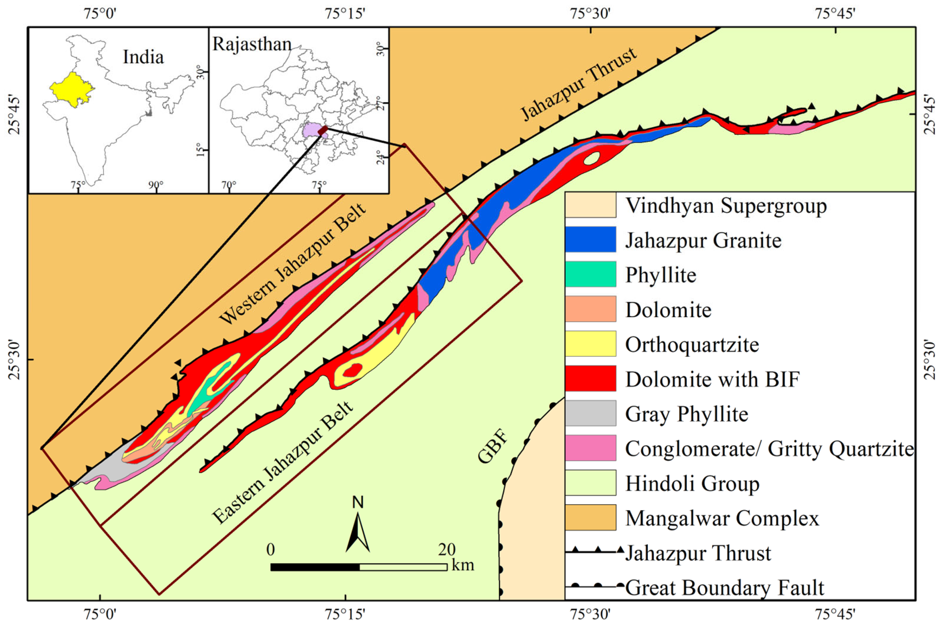
2. Study Area
3. Materials and Methodology
3.1. Materials
3.2. Mineral Mapping
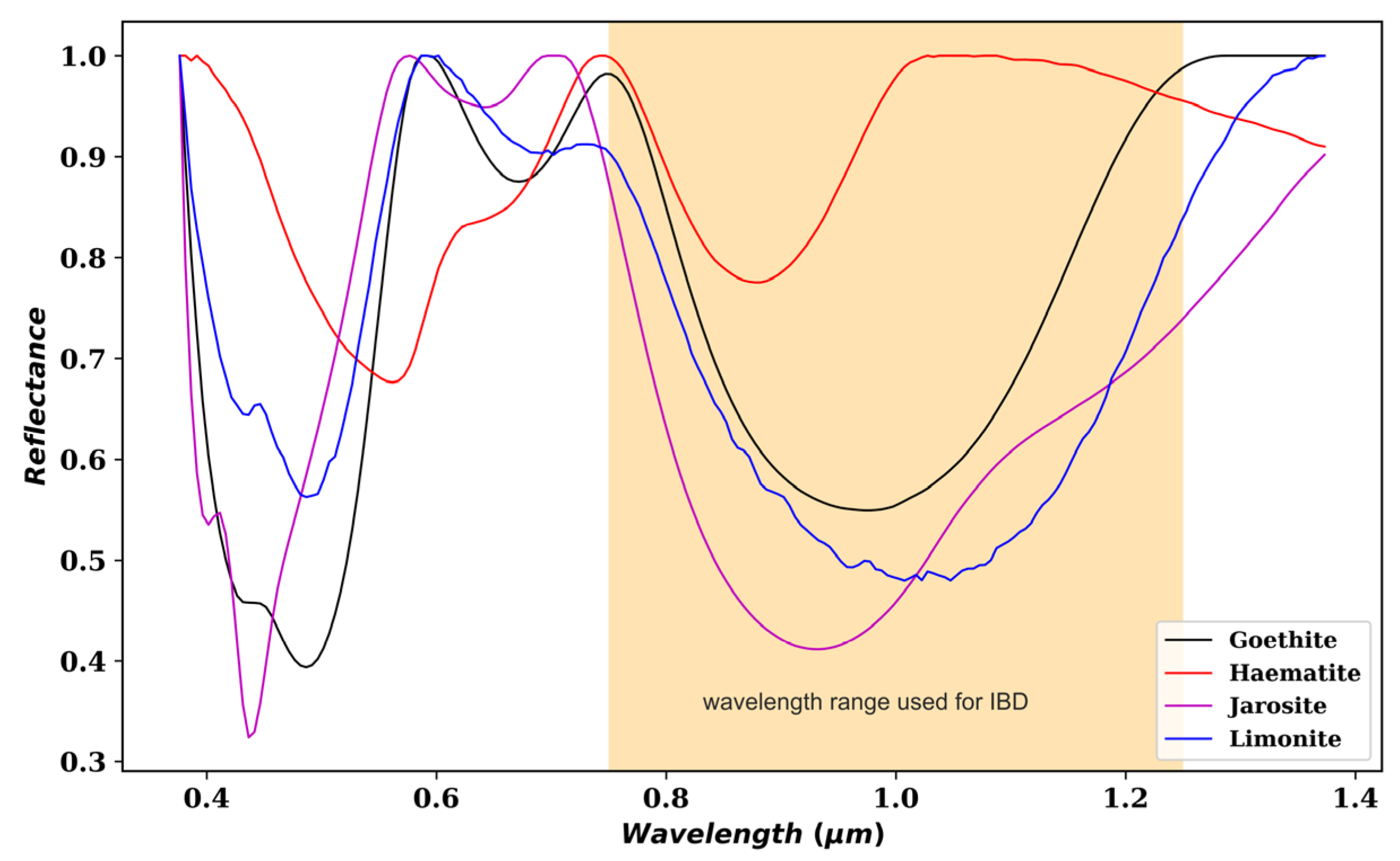
3.3. Integrated Band Depth
3.4. Masking
4. Results
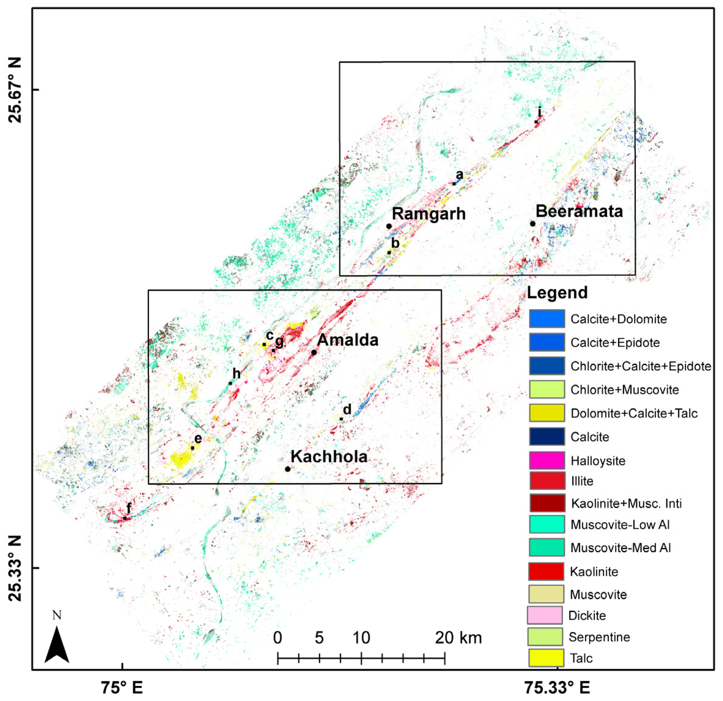
4.1. Mineral Map
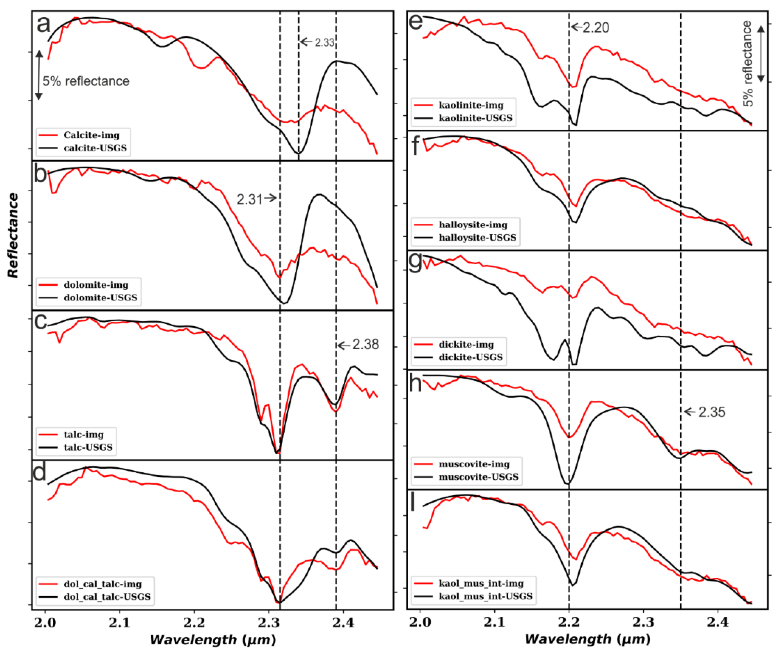
4.2. Validation of Mineral Map
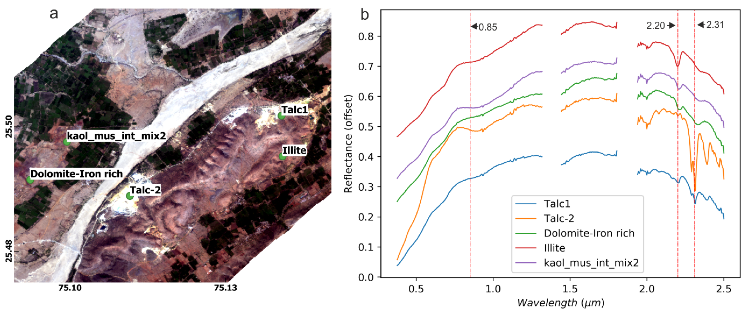
4.3. Spectroscopic Characterization of Mineralized Area
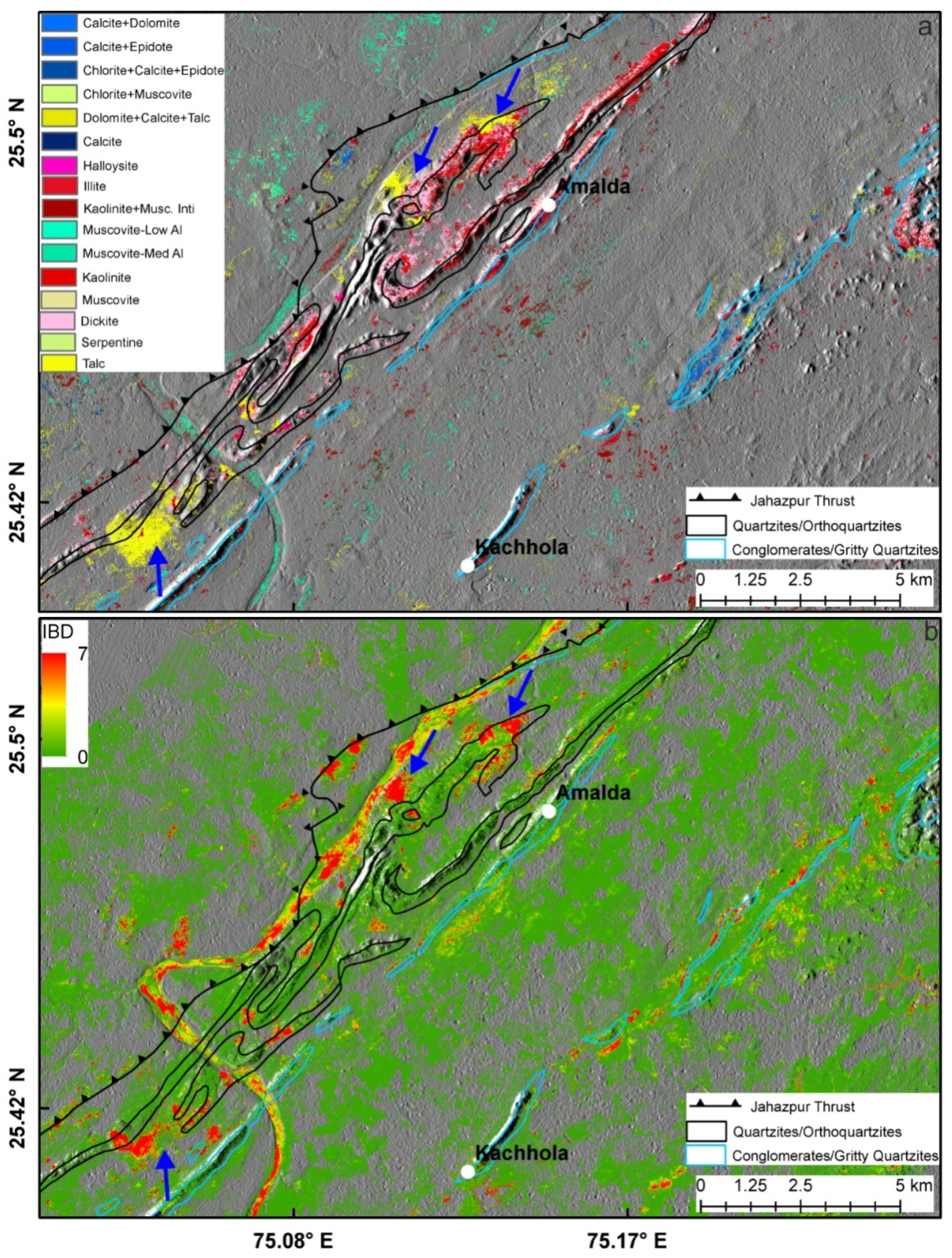
4.4. Geological and Mineralogical Control of Talc Mineralization
4.4.1. Amalda Area
4.4.2. Ramgarh Area
5. Discussion
5.1. Imagining Spectroscopy for Mapping Spectrally Similar Minerals
5.2. Mechanism of Talc Formation
6. Conclusions
Author Contributions
Funding
Data Availability Statement
Acknowledgments
Conflicts of Interest
References
- Ali-Bik, M.W.; Hassan, S.M.; Sadek, M.F. Volcanogenic Talc-Copper Deposits of Darhib-Abu Jurdi Area, Egypt: Petrogenesis and Remote Sensing Characterization. Geol. J. 2020, 55, 5330–5354. [Google Scholar] [CrossRef]
- Abrams, M.; Yamaguchi, Y. Twenty Years of ASTER Contributions to Lithologic Mapping and Mineral Exploration. Remote Sens. 2019, 11, 1394. [Google Scholar] [CrossRef]
- Pour, A.B.; Hashim, M. The Application of ASTER Remote Sensing Data to Porphyry Copper and Epithermal Gold Deposits. Ore Geol. Rev. 2012, 44, 1–9. [Google Scholar] [CrossRef]
- Zhang, X.; Pazner, M.; Duke, N. Lithologic and Mineral Information Extraction for Gold Exploration Using ASTER Data in the South Chocolate Mountains (California). ISPRS J. Photogramm. Remote Sens. 2007, 62, 271–282. [Google Scholar] [CrossRef]
- Bedini, E. Mineral Mapping in the Kap Simpson Complex, Central East Greenland, Using HyMap and ASTER Remote Sensing Data. Adv. Space Res. 2011, 47, 60–73. [Google Scholar] [CrossRef]
- Hewson, R.D.; Cudahy, T.J.; Mizuhiko, S.; Ueda, K.; Mauger, A.J. Seamless Geological Map Generation Using ASTER in the Broken Hill-Curnamona Province of Australia. Remote Sens. Environ. 2005, 99, 159–172. [Google Scholar] [CrossRef]
- Rowan, L.C.; Mars, J.C. Lithologic Mapping in the Mountain Pass, California Area Using Advanced Spaceborne Thermal Emission and Reflection Radiometer (ASTER) Data. Remote Sens. Environ. 2003, 84, 350–366. [Google Scholar] [CrossRef]
- Jain, R.; Bhu, H.; Purohit, R. Mapping of the Silica-Rich Rocks and Serpentinites Using Newly Defined Thermal Indices from Advanced Spaceborne Thermal Emission and Reflection Radiometer Thermal Infrared Data of Udaipur-Rakhabdev Region, Rajasthan, India. J. Appl. Remote Sens. 2022, 16, 034501. [Google Scholar] [CrossRef]
- Jain, R. Presence of Base Metals in the Southern Extension of Zawarmala Dolomite, Udaipur, Rajasthan, India. Curr. Sci. 2021, 121, 962–966. [Google Scholar] [CrossRef]
- Jain, R.; Bhu, H.; Purohit, R. ASTER Remote Sensing Data for Delineation of Base Metal—Bearing Dolomites in South-East of Aravalli Craton, India. Arab. J. Geosci. 2022, 15, 1620. [Google Scholar] [CrossRef]
- Guha, A.; Yamaguchi, Y.; Chatterjee, S.; Rani, K.; Vinod Kumar, K. Emittance Spectroscopy and Broadband Thermal Remote Sensing Applied to Phosphorite and Its Utility in Geoexploration: A Study in the Parts of Rajasthan, India. Remote Sens. 2019, 11, 1003. [Google Scholar] [CrossRef]
- Rajendran, S.; Hersi, O.S.; Al-Harthy, A.; Al-Wardi, M.; El-Ghali, M.A.; Al-Abri, A.H. Capability of Advanced Spaceborne Thermal Emission and Reflection Radiometer (ASTER) on Discrimination of Carbonates and Associated Rocks and Mineral Identification of Eastern Mountain Region (Saih Hatat Window) of Sultanate of Oman. Carbonates Evaporites 2011, 26, 351–364. [Google Scholar] [CrossRef]
- Gabr, S.; Ghulam, A.; Kusky, T. Detecting Areas of High-Potential Gold Mineralization Using ASTER Data. Ore Geol. Rev. 2010, 38, 59–69. [Google Scholar] [CrossRef]
- de Souza Filho, C.R.; Tapia, C.H.; Crósta, A.P.; Xavier, R.P. Infrared Spectroscopy and ASTER Imagery Analysis of Hydrothermal Alteration Zones at the Quellaveco Porphyry-Cooper Deposit, Southern Peru. In Proceedings of the American Society of Photogrammetry and Remote Sensing (ASPRS), Annual Conference—“Technology: Converging at the Top of the World”, Anchorage, AK, USA, 5–9 May 2003; pp. 1–12. [Google Scholar]
- Jain, R.; Bhu, H.; Kumar, H.; Purohit, R. Integration of Multi-Sensor Remote Sensing, Geological and Geochemical Data for Delineation of Pb–Zn Bearing Carbonates of Middle Aravalli Group in Zawar–Dungarpur Belt, NW India. Geocarto Int. 2022, 37, 17165–17199. [Google Scholar] [CrossRef]
- Fereydooni, H.; Mojeddifar, S. A Directed Matched Filtering Algorithm (DMF) for Discriminating Hydrothermal Alteration Zones Using the ASTER Remote Sensing Data. Int. J. Appl. Earth Obs. Geoinf. 2017, 61, 1–13. [Google Scholar] [CrossRef]
- Ramakrishnan, D.; Bharti, R. Hyperspectral Remote Sensing and Geological Applications. Curr. Sci. 2015, 108, 879–891. [Google Scholar]
- Kumar, H.; Rajawat, A.S. Aqueous Alteration Mapping in Rishabdev Ultramafic Complex Using Imaging Spectroscopy. Int. J. Appl. Earth Obs. Geoinf. 2020, 88, 102084. [Google Scholar] [CrossRef]
- Jain, R.; Sharma, R.U. Airborne Hyperspectral Data for Mineral Mapping in Southeastern Rajasthan, India. Int. J. Appl. Earth Obs. Geoinf. 2019, 81, 137–145. [Google Scholar] [CrossRef]
- Jain, R.; Bhu, H.; Purohit, R. Airborne Imaging Spectrometer Dataset for Spectral Characterization and Predictive Mineral Mapping Using Sub-Pixel Based Classifier in Parts of Udaipur, Rajasthan, India. Adv. Space Res. 2022, in press. [Google Scholar] [CrossRef]
- Thompson, D.R.; Braverman, A.; Brodrick, P.G.; Candela, A.; Carmon, N.; Clark, R.N.; Connelly, D.; Green, R.O.; Kokaly, R.F.; Li, L.; et al. Quantifying Uncertainty for Remote Spectroscopy of Surface Composition. Remote Sens. Environ. 2020, 247, 111898. [Google Scholar] [CrossRef]
- Swayze, G.A.; Kokaly, R.F.; Higgins, C.T.; Clinkenbeard, J.P.; Clark, R.N.; Lowers, H.A.; Sutley, S.J. Mapping Potentially Asbestos-Bearing Rocks Using Imaging Spectroscopy. Geology 2009, 37, 763–766. [Google Scholar] [CrossRef]
- Goetz, A.F.H. Three Decades of Hyperspectral Remote Sensing of the Earth: A Personal View. Remote Sens. Environ. 2009, 113, S5–S16. [Google Scholar] [CrossRef]
- Hunt, G.W.; Salisbury, J.R. Visible and Near Infrared Spectra of Minerals and Rocks. I. Silicate Minerals. Mod. Geol. 1970, 1, 283–300. [Google Scholar]
- Guha, A.; Ghosh, U.K.; Sinha, J.; Pour, A.B.; Bhaisal, R.; Chatterjee, S.; Baranval, N.K.; Rani, N.; Vinod Kumar, K.; Rao, P.V.N. Potentials of Airborne Hyperspectral AVIRIS-NG Data in the Exploration of Base Metal Deposit—A Study in the Parts of Bhilwara, Rajasthan. Remote Sens. 2021, 13, 2101. [Google Scholar] [CrossRef]
- Guha, A.; Chatterjee, S.; Oommen, T.; Vinod Kumar, K.; Roy, S.K. Synergistic Use of ASTER, L-Band ALOS PALSAR, and Hyperspectral AVIRIS-NG Data for Exploration of Lode Type Gold Deposit—A Study in Hutti Maski Schist Belt, India. Ore Geol. Rev. 2021, 128, 103818. [Google Scholar] [CrossRef]
- Wan, Y.-q.; Fan, Y.-h.; Jin, M.-s. Application of Hyperspectral Remote Sensing for Supplementary Investigation of Polymetallic Deposits in Huaniushan Ore Region, Northwestern China. Nat. Sci. Rep. 2021, 11, 440. [Google Scholar] [CrossRef]
- Pour, A.B.; Zoheir, B.; Pradhan, B.; Hashim, M. Editorial for the Special Issue: Multispectral and Hyperspectral Remote Sensing Data for Mineral Exploration and Environmental Monitoring of Mined Areas. Remote Sens. 2021, 13, 519. [Google Scholar] [CrossRef]
- Bedini, E.; Chen, J. Application of PRISMA Satellite Hyperspectral Imagery to Mineral Alteration Mapping at Cuprite, Nevada, USA. J. Hyperspectral Remote Sens. 2020, 10, 87–94. [Google Scholar] [CrossRef]
- van Ruitenbeek, F.J.A.; Cudahy, T.; Hale, M.; van der Meer, F.D. Tracing Fluid Pathways in Fossil Hydrothermal Systems with Near-Infrared Spectroscopy. Geology 2005, 33, 597. [Google Scholar] [CrossRef]
- Bedini, E. The Use of Hyperspectral Remote Sensing for Mineral Exploration: A Review. J. Hyperspectral Remote Sens. 2017, 7, 189–211. [Google Scholar] [CrossRef]
- Swayze, G.A.; Smith, K.S.; Clark, R.N.; Sutley, S.J.; Pearson, R.M.; Vance, J.S.; Hageman, P.L.; Briggs, P.H.; Meier, A.L.; Singleton, M.J.; et al. Using Imaging Spectroscopy to Map Acidic Mine Waste. Environ. Sci. Technol. 2000, 34, 47–54. [Google Scholar] [CrossRef]
- Roache, T.J.; Walshe, J.L.; Huntington, J.F.; Quigley, M.A.; Yang, K.; Bil, B.W.; Blake, K.L.; Hyvärinen, T. Epidote—Clinozoisite as a Hyperspectral Tool in Exploration for Archean Gold. Aust. J. Earth Sci. 2011, 58, 813–822. [Google Scholar] [CrossRef]
- Keeling, J.; Mauger, A.; Raven, M. Airborne Hyperspectral Survey and Kimberlite Detection in the Terowie District, South Australia. In Proceedings of the CRC LEME Regional Regolith Symposia, Adelaide, SA, Australia, 10–26 November 2004; pp. 166–170. [Google Scholar]
- Booysen, R.; Lorenz, S.; Thiele, S.T.; Fuchsloch, W.C.; Marais, T.; Nex, P.A.M.; Gloaguen, R. Accurate Hyperspectral Imaging of Mineralised Outcrops: An Example from Lithium-Bearing Pegmatites at Uis, Namibia. Remote Sens. Environ. 2022, 269, 112790. [Google Scholar] [CrossRef]
- Khan, S.D.; Jacobson, S. Remote Sensing and Geochemistry for Detecting Hydrocarbon Microseepages. Geol. Soc. Am. Bull. 2008, 120, 96–105. [Google Scholar] [CrossRef]
- Thompson, D.R.; Thorpe, A.K.; Frankenberg, C.; Green, R.O.; Duren, R.; Guanter, L.; Hollstein, A.; Middleton, E.; Ong, L.; Ungar, S. Space-Based Remote Imaging Spectroscopy of the Aliso Canyon CH4 Superemitter. Geophys. Res. Lett. 2016, 43, 6571–6578. [Google Scholar] [CrossRef]
- Roberts, D.A.; Bradley, E.S.; Cheung, R.; Leifer, I.; Dennison, P.E.; Margolis, J.S. Mapping Methane Emissions from a Marine Geological Seep Source Using Imaging Spectrometry. Remote Sens. Environ. 2010, 114, 592–606. [Google Scholar] [CrossRef]
- Heller Pearlshtien, D.; Pignatti, S.; Greisman-Ran, U.; Ben-Dor, E. PRISMA Sensor Evaluation: A Case Study of Mineral Mapping Performance over Makhtesh Ramon, Israel. Int. J. Remote Sens. 2021, 42, 5882–5914. [Google Scholar] [CrossRef]
- Pignatti, S.; Palombo, A.; Pascucci, S.; Romano, F.; Santini, F.; Simoniello, T.; Umberto, A.; Vincenzo, C.; Acito, N.; Diani, M.; et al. The PRISMA Hyperspectral Mission: Science Activities and Opportunities for Agriculture and Land Monitoring. In Proceedings of the 2013 IEEE International Geoscience and Remote Sensing Symposium—IGARSS, Melbourne, VI, Australia, 21–26 July 2013; IEEE: Piscataway, NJ, USA, 2013; pp. 4558–4561. [Google Scholar]
- Tripathi, P.; Garg, R.D. First Impressions from the PRISMA Hyperspectral Mission. Curr. Sci. 2020, 119, 1267–1281. [Google Scholar] [CrossRef]
- Laukamp, C. Geological Mapping Using Mineral Absorption Feature-Guided Band-Ratios Applied to Prisma Satellite Hyperspectral Level 2D Imagery. In Proceedings of the IGARSS 2022—2022 IEEE International Geoscience and Remote Sensing Symposium, Kuala Lumpur, Malaysia, 17 July 2022; IEEE: Piscataway, NJ, USA, 2013; pp. 5981–5984. [Google Scholar]
- Nieke, J.; Rast, M. Towards the Copernicus Hyperspectral Imaging Mission for the Environment (CHIME). In Proceedings of the IGARSS 2018—2018 IEEE International Geoscience and Remote Sensing Symposium, Valencia, Spain, 22–27 July 2018; IEEE: Piscataway, NJ, USA; pp. 157–159. [Google Scholar]
- Lee, C.M.; Cable, M.L.; Hook, S.J.; Green, R.O.; Ustin, S.L.; Mandl, D.J.; Middleton, E.M. An Introduction to the NASA Hyperspectral InfraRed Imager (HyspIRI) Mission and Preparatory Activities. Remote Sens. Environ. 2015, 167, 6–19. [Google Scholar] [CrossRef]
- GSI. Geology and Mineral Resources of Rajasthan, 3rd ed.; Miscellenous Publication No. 30, Part 12; Geological Survey of India: Jaipur, India, 2011. [Google Scholar]
- Jain, R.; Sharma, R.U. Mapping of Mineral Zones Using the Spectral Feature Fitting Method in Jahazpur Belt, Rajasthan, India. Int. Res. J. Eng. Technol. 2018, 5, 562–567. [Google Scholar]
- Gupta, S.N.; Arora, Y.K.; Mathur, R.K.; Iqballuddin; Prasad, B.; Sahai, T.N.; Sharma, S.B. The Precambrian Geology of the Aravalli Region, Southern Rajasthan & North-Eastern Gujarat. Mem. Geol. Surv. India 1997, 123, 1–262. [Google Scholar]
- Roy, A.B.; Jakhar, S.R. Geology of Rajasthan (Northwest India): Precambrian to Recent; Scientific Publishers: Jodhpur, India, 2002; ISBN 81-7233-304-8. [Google Scholar]
- Sinha-Roy, S.; Malhotra, G.; Mohanty, M. Geology of Rajasthan, 2nd ed.; Geological Society of India: Bangalore, India, 2013. [Google Scholar]
- Tripathi, M.K.; Govil, H. Regolith Mapping and Geochemistry of Hydrothermally Altered, Weathered and Clay Minerals, Western Jahajpur Belt, Bhilwara, India. Geocarto Int. 2020, 37, 879–895. [Google Scholar] [CrossRef]
- Bhadra, B.K.; Pathak, S.; Nanda, D.; Gupta, A.; Srinivasa Rao, S. Spectral Characteristics of Talc and Mineral Abundance Mapping in the Jahazpur Belt of Rajasthan, India Using AVIRIS-NG Data. Int. J. Remote Sens. 2020, 41, 8754–8774. [Google Scholar] [CrossRef]
- Tripathi, M.K.; Govil, H.; Chattoraj, S.L. Identification of Hydrothermal Altered/Weathered and Clay Minerals through Airborne AVIRIS-NG Hyperspectral Data in Jahajpur, India. Heliyon 2020, 6, e03487. [Google Scholar] [CrossRef]
- Sunshine, J.M.; Farnham, T.L.; Feaga, L.M.; Groussin, O.; Merlin, F.; Milliken, R.E.; A’Hearn, M.F. Temporal and Spatial Variability of Lunar Hydration as Observed by the Deep Impact Spacecraft. Science 2009, 326, 565–568. [Google Scholar] [CrossRef]
- Pieters, C.M.; Goswami, J.N.; Clark, R.N.; Annadurai, M.; Boardman, J.; Buratti, B.; Combe, J.-P.; Dyar, M.D.; Green, R.; Head, J.W.; et al. Character and Spatial Distribution of OH/H2O on the Surface of the Moon Seen by M3 on Chandrayaan-1. Science 2009, 326, 568–572. [Google Scholar] [CrossRef] [PubMed]
- Verma, P.K. Deep Continental Structures and Processes in the Aravalli Mountain Range, NW India: Focuson Evolution and Inversion of Regional Faults. News Lett. DST Gov. India 1999, 9, 197–212. [Google Scholar]
- Gupta, S.N.; Arora, Y.K.; Mathur, R.K.; Iqballuddin; Prasad, B.; Sahai, T.N.; Sharma, S.B. Lithostratigraphic Map of Aravalli Region, Southern Rajasthan & Northern Gujarat; Geological Survey: Hyderabad, India, 1980. [Google Scholar]
- Mohanty, M.; Guha, D. Lithotectonostratigraphy of the Dismembered Greenstone Sequence of the Mangalwar Complex around Lawa Sardargarh and Parvali Nareas, Rajsamand District, Rajasthan. In Continental Crust of Northwestern and Central India; Sinha-Roy, S., Gupta, K.R., Eds.; Memoir of Geological Society of India: Jaipur, India, 1995; Volume 31, pp. 141–162. [Google Scholar]
- Reddy, P.R.; Prasad, B.R.; Rao, V.V.; Khare, P.; Rao, G.K.; Murthy, A.S.N.; Sarkar, D.; Raju, S.; Rao, G.S.P.; Sridhar, V. Deep Seismic Reflection Profiling along Nandsi-Kunjer Section of Nagaur-Jhalawar Transect: Preliminary Results. In Continental Crust of Northwestern and Central India; Sinha-Roy, S., Gupta, K.R., Eds.; Memoir of Geological Society of India: Jaipur, India, 1995; pp. 353–372. [Google Scholar]
- Sinha-Roy, S.; Malhotra, G.; Mohanty, M. Geology of Rajasthan; Geological Society of India: Bangalore, India, 1998; ISBN 81-85867-27-5. [Google Scholar]
- Roy, A.B.; Purohit, R. Indian Shield: Precambrian Evolution and Phanerozoic Reconstitution, 1st ed.; Elsevier Inc.: Cambridge, MA, USA, 2018; ISBN 9780128098394. [Google Scholar]
- Pandit, M.K.; Sial, A.N.; Malhotra, G.; Shekhawat, L.S.; Ferreira, V.P. C-, O-Isotope and Whole-Rock Geochemistry of Proterozoic Jahazpur Carbonates, NW Indian Craton. Gondwana Res. 2003, 6, 513–522. [Google Scholar] [CrossRef]
- Sengupta, S.; Basak, K. Mesoproterozoic Orogeny along the Eastern Boundary of Aravalli Craton, Northwestern India: A Structural and Geochronological Study of Hindoli-Jahazpur Group of Rocks. J. Earth Syst. Sci. 2021, 130, 203. [Google Scholar] [CrossRef]
- Thompson, D.R.; Gao, B.C.; Green, R.O.; Roberts, D.A.; Dennison, P.E.; Lundeen, S.R. Atmospheric Correction for Global Mapping Spectroscopy: ATREM Advances for the HyspIRI Preparatory Campaign. Remote Sens. Environ. 2015, 167, 64–77. [Google Scholar] [CrossRef]
- Mishra, M.K.; Gupta, A.; John, J.; Shukla, B.P.; Dennison, P.; Srivastava, S.S.; Kaushik, N.K.; Misra, A.; Dhar, D. Retrieval of Atmospheric Parameters and Data-Processing Algorithms for AVIRIS-NG Indian Campaign Data. Curr. Sci. 2019, 116, 1089–1100. [Google Scholar] [CrossRef]
- Clark, R.N.; Swayze, G.A.; Livo, K.E.; Kokaly, R.F.; Sutley, S.J.; Dalton, J.B.; McDougal, R.R.; Gent, C.A. Imaging Spectroscopy: Earth and Planetary Remote Sensing with the USGS Tetracorder and Expert Systems. J. Geophys. Res. 2003, 108, 5131. [Google Scholar] [CrossRef]
- Kokaly, R.F.; Clark, R.N.; Swayze, G.A.; Livo, K.E.; Hoefen, T.M.; Pearson, N.C.; Wise, R.A.; Benzel, W.M.; Lowers, H.A.; Driscoll, R.L.; et al. USGS Spectral Library, Version 7. U.S. Geological Survey Data Series 1035, U.S. Geological Survey: Reston, VA, USA, 2017. [CrossRef]
- Richter, R. Correction of Atmospheric and Topographic Effects for High Spatial Resolution Satellite Imagery. Int. J. Remote Sens. 1997, 18, 1099–1111. [Google Scholar] [CrossRef]
- Clark, R.N.; Roush, T.L. Reflectance Spectroscopy: Quantitative Analysis Techniques for Remote Sensing Applications. J. Geophys. Res. Solid Earth 1984, 89, 6329–6340. [Google Scholar] [CrossRef]
- Mustard, J.F.; Pieters, C.M.; Isaacson, P.J.; Head, J.W.; Besse, S.; Clark, R.N.; Klima, R.L.; Petro, N.E.; Staid, M.I.; Sunshine, J.M.; et al. Compositional Diversity and Geologic Insights of the Aristarchus Crater from Moon Mineralogy Mapper Data. J. Geophys. Res. 2011, 116, E00G12. [Google Scholar] [CrossRef]
- Nettles, J.W.; Staid, M.; Besse, S.; Boardman, J.; Clark, R.N.; Dhingra, D.; Isaacson, P.; Klima, R.; Kramer, G.; Pieters, C.M.; et al. Optical Maturity Variation in Lunar Spectra as Measured by Moon Mineralogy Mapper Data. J. Geophys. Res. 2011, 116, E00G17. [Google Scholar] [CrossRef]
- Gaffey, S.J. Spectral Reflectance of Carbonate Minerals in the Visible and near Infrared (0.35-2.55 Microns); Calcite, Aragonite, and Dolomite. Am. Mineral. 1986, 71, 151–162. [Google Scholar]
- Petit, S.; Martin, F.; Wiewiora, A.; De Parseval, P.; Decarreau, A. Crystal-Chemistry of Talc: A Near Infrared (NIR) Spectroscopy Study. Am. Mineral. 2004, 89, 319–326. [Google Scholar] [CrossRef]
- Michalski, J.R.; Cuadros, J.; Bishop, J.L.; Darby Dyar, M.; Dekov, V.; Fiore, S. Constraints on the Crystal-Chemistry of Fe/Mg-Rich Smectitic Clays on Mars and Links to Global Alteration Trends. Earth Planet. Sci. Lett. 2015, 427, 215–225. [Google Scholar] [CrossRef]
- Cuadros, J.; Dekov, V.M.; Fiore, S. Crystal Chemistry of the Mixed-Layer Sequence Talc-Talc-Smectite-Smectite from Submarine Hydrothermal Vents. Am. Mineral. 2008, 93, 1338–1348. [Google Scholar] [CrossRef]
- Pineau, M.; Mathian, M.; Baron, F.; Rondeau, B.; Le Deit, L.; Allard, T.; Mangold, N. Estimating Kaolinite Crystallinity Using Near-Infrared Spectroscopy: Implications for Its Geology on Earth and Mars. Am. Mineral. 2022, 107, 1453–1469. [Google Scholar] [CrossRef]
- Holm, N.G.; Oze, C.; Mousis, O.; Waite, J.H.; Guilbert-Lepoutre, A. Serpentinization and the Formation of H2 and CH4 on Celestial Bodies (Planets, Moons, Comets). Astrobiology 2015, 15, 587–600. [Google Scholar] [CrossRef] [PubMed]
- Hecht, L.; Freiberger, R.; Gilg, H.A.; Grundmann, G.; Kostitsyn, Y.A. Rare Earth Element and Isotope (C, O, Sr) Characteristics of Hydrothermal Carbonates: Genetic Implications for Dolomite-Hosted Talc Mineralization at Gopfersgrun (Fichtelgebirge, Germany). Chem. Geol. 1999, 155, 115–130. [Google Scholar] [CrossRef]
- Swayze, G.A.; Clark, R.N.; Goetz, A.F.H.; Livo, K.E.; Breit, G.N.; Kruse, F.A.; Sutley, S.J.; Snee, L.W.; Lowers, H.A.; Post, J.L.; et al. Mapping Advanced Argillic Alteration at Cuprite, Nevada, Using Imaging Spectroscopy. Econ. Geol. 2014, 109, 1179–1221. [Google Scholar] [CrossRef]
- Heylen, R.; Gader, P. Nonlinear Spectral Unmixing With a Linear Mixture of Intimate Mixtures Model. IEEE Geosci. Remote Sens. Lett. 2014, 11, 1195–1199. [Google Scholar] [CrossRef]
- Ducasse, E.; Adeline, K.; Briottet, X.; Hohmann, A.; Bourguignon, A.; Grandjean, G. Montmorillonite Estimation in Clay-Quartz-Calcite Samples from Laboratory SWIR Imaging Spectroscopy: A Comparative Study of Spectral Preprocessings and Unmixing Methods. Remote Sens. 2020, 12, 1723. [Google Scholar] [CrossRef]
- Wang, D.; Shi, Z.; Cui, X. Robust Sparse Unmixing for Hyperspectral Imagery. IEEE Trans. Geosci. Remote Sens. 2018, 56, 1348–1359. [Google Scholar] [CrossRef]
- El-Sharkawy, M.F. Talc Mineralization of Ultramafic Affinity in the Eastern Desert of Egypt. Miner. Depos. 2000, 35, 346–363. [Google Scholar] [CrossRef]
- Joshi, P.; Pant, P.D.; Upadhyaya, R.C. Petrography and Geochemistry of Magnesite and Talc Deposits of Jhiroli, Kumaun Lesser Himalaya. In Magmatism, Tectonism And Mineralization; Kumar, S., Ed.; Macmillan Publishers India Ltd.: New Delhi, India, 2009. [Google Scholar]
- Winter, J.D. An Introduction to Igneous and Metamorphic Petrology, 1st ed.; Pearson College Div: Prentice Hall Upper Saddle River, NJ, USA, 2001. [Google Scholar]
- Dey, B.; Das, K.; Dasgupta, N.; Bose, S.; Hidaka, H.; Ghatak, H. Zircon U-Pb (SHRIMP) Ages of the Jahazpur Granite and Mangalwar Gneiss from the Deoli-Jahazpur Sector, Rajasthan, NW India: A Preliminary Reappraisal of Stratigraphic Correlation and Implications to Crustal Growth. In Geological Evolution of the Precambrian Indian Shield. Society of Earth Scientists Series; Mondal, M.E.A., Ed.; Springer: Cham, Switzerland, 2019; pp. 39–56. [Google Scholar]
- Klein, C.; Ladeira, E.A. Geochemistry and Petrology of Some Proterozoic Banded Iron-Formations of the Quadrilatero Ferrifero, Minas Gerais, Brazil. Econ. Geol. 2000, 95, 405–427. [Google Scholar] [CrossRef]
- Bau, M.; Möller, P. Rare Earth Element Systematics of the Chemically Precipitated Component in Early Precambrian Iron Formations and the Evolution of the Terrestrial Atmosphere-Hydrosphere-Lithosphere System. Geochim. Cosmochim. Acta 1993, 57, 2239–2249. [Google Scholar] [CrossRef]
- Shin, D.; Lee, I. The Fluid Evolution Related to Talc Mineralization in the Hwanggangri Area, South Korea. Resour. Geol. 2002, 52, 273–278. [Google Scholar] [CrossRef]
- Anderson, D.L.; Mogk, D.W.; Childs, J.F. Petrogenesis and Timing of Talc Formation in the Ruby Range, Southwestern Montana. Econ. Geol. 1990, 85, 585–600. [Google Scholar] [CrossRef]


Disclaimer/Publisher’s Note: The statements, opinions and data contained in all publications are solely those of the individual author(s) and contributor(s) and not of MDPI and/or the editor(s). MDPI and/or the editor(s) disclaim responsibility for any injury to people or property resulting from any ideas, methods, instructions or products referred to in the content. |
© 2023 by the authors. Licensee MDPI, Basel, Switzerland. This article is an open access article distributed under the terms and conditions of the Creative Commons Attribution (CC BY) license (https://creativecommons.org/licenses/by/4.0/).
Share and Cite
Kumar, H.; Ramakrishnan, D.; Jain, R.; Govil, H. Can Imaging Spectroscopy Divulge the Process Mechanism of Mineralization? Inferences from the Talc Mineralization, Jahazpur, India. Remote Sens. 2023, 15, 2394. https://doi.org/10.3390/rs15092394
Kumar H, Ramakrishnan D, Jain R, Govil H. Can Imaging Spectroscopy Divulge the Process Mechanism of Mineralization? Inferences from the Talc Mineralization, Jahazpur, India. Remote Sensing. 2023; 15(9):2394. https://doi.org/10.3390/rs15092394
Chicago/Turabian StyleKumar, Hrishikesh, Desikan Ramakrishnan, Ronak Jain, and Himanshu Govil. 2023. "Can Imaging Spectroscopy Divulge the Process Mechanism of Mineralization? Inferences from the Talc Mineralization, Jahazpur, India" Remote Sensing 15, no. 9: 2394. https://doi.org/10.3390/rs15092394