Article

Evaluating the Performance of PRISMA Shortwave Infrared Imaging Sensor for Mapping Hydrothermally Altered and Weathered Minerals Using the Machine Learning Paradigm

1
Department of Computer Applications, National Institute of Technology Raipur, Raipur 492010, India
2
Department of Applied Geology, National Institute of Technology Raipur, Raipur 492010, India
3
Department of Geology, University of Delhi, New Delhi 110007, India
4
Remote Sensing Laboratory, Institute of Environment and Sustainable Development, Banaras Hindu University, Varanasi 221005, India
*
Author to whom correspondence should be addressed.
Remote Sens. 2023, 15(12), 3133; https://doi.org/10.3390/rs15123133
Submission received: 1 May 2023 / Revised: 8 June 2023 / Accepted: 8 June 2023 / Published: 15 June 2023
(This article belongs to the Special Issue The Use of Hyperspectral Remote Sensing Data in Mineral Exploration)

Abstract

:
Satellite images provide consistent and frequent information that can be used to estimate mineral resources over a large spatial extent. Advances in spaceborne hyperspectral remote sensing (HRS) and machine learning can help to support various remote-sensing-based applications, including mineral exploration. Leveraging these advances, the present study evaluates recently launched PRISMA spaceborne satellite images to map hydrothermally altered and weathered minerals using various machine-learning-based classification algorithms. The study was performed for the town of Jahazpur in Rajasthan, India (75°06′23.17″E, 25°25′23.37″N). The distribution map for minerals such as kaolinite, talc, and montmorillonite was generated using the spectral angle mapper technique. The resultant mineral distribution map was verified through an intensive field validation survey on surface exposures of the minerals. Furthermore, the obtained pixels of the end-members were used to develop the machine-learning-based classification models. Measures such as accuracy, kappa coefficient, F1 score, precision, recall, and ROC curve were employed to evaluate the performance of developed models. The results show that the stochastic gradient descent and artificial-neural-network-based multilayer perceptron classifiers were more accurate than other algorithms. Results confirm that the PRISMA dataset has enormous potential for mineral mapping in mountainous regions utilizing a machine-learning-based classification framework.

Graphical Abstract

1. Introduction

Hyperspectral remote sensing (HRS) has the unique capability of concurrently acquiring the image and spectral information of the target objects. The acquired images comprise hundreds of contiguous and narrow-bandwidth spectral image bands in the VNIR-SWIR range. Therefore, they are widely used to obtain quantitative information in various fields such as agriculture, forestry, oceanology, lithology, environmental studies, defense applications, and urban planning [1]. Mineral prospectivity mapping (MPM) is essential for further exploration and natural resource management. Each mineral resource depicts a specific spectral characteristic based on its chemical bonding and physical features in the spectral range of 0.4–2.5 µm [2]. The pixels of hyperspectral images (HSI) correspond to a spectral vector of reflectance values in this specific wavelength region, making it possible to derive spectral characteristics of the mineral objects of the representative image pixel. Multispectral remote sensing captures reflected energy in broader and a limited number of spectral bands [3]. As a result, different minerals may have similar spectral characteristics when observed with the conventional multispectral images (MSI). Therefore, emerging HRS with contiguous and rich spectral features better characterizes mineral resources than multispectral remote sensing.
HRS technology is still in the developing stage despite various technological advancements. Various hyperspectral sensors inundated mineral exploration applications recently, and can be categorized as follows: 1. Airborne hyperspectral sensors (e.g., airborne visible/infrared imaging spectrometer-next generation (AVIRIS-NG)); 2. Spaceborne hyperspectral sensors (e.g., Hyperion); 3. Hyperspectral sensors mounted on unmanned aerial vehicles (e.g., BaySpec OCI-D2000); 4. Handheld spectral sensors (e.g., analytical spectral devices) [4]. Spaceborne HRS makes the technology more available to the research community. The Hyperion spaceborne hyperspectral remote sensor was launched in November 2000 and decommissioned in 2017 [5]. It collected ground data in 224 spectral bands with 30 m spatial resolution and 7.5 m swath width. Despite its short operating lifespan, it paved the way for technological advances in spaceborne hyperspectral sensors. The PRISMA spaceborne hyperspectral sensor is developed by the Italian Space Agency i.e., ASI. It was launched on 22 March 2019, into a sun-synchronous orbit with a 29-day relook period [6]. It facilitates imageries with an improved signal-to-noise ratio (SNR) than the Hyperion hyperspectral remote sensor. It is basically a satellite-based earth observation mission aimed at delivering spectroscopic imageries to foster novel methods and applications for managing and analyzing natural resources. Section 3 provides observational details of the PRISMA dataset.
In real geographic scenarios, minerals with similar spectral properties can be mixed. In such scenarios, the spectral absorption region of minerals overlaps with each other, and spectra become highly correlated. Due to light scattering effects, the same type of mineral may pose different spectral signatures. The correlation among the spectra, light scattering effects, substantial number of spectral features, a limited collection of ground samples, and the complex spectral pattern of surface mineral objects hinders the performance of traditional identification and classification algorithms.
Machine learning algorithms (MLAs) can effectively address these limitations in a complex and high-dimensional hyperspectral-image-based mineral exploration. Machine learning algorithms (MLAs) can adequately capture (during training) the spectral patterns from a specific dataset for future predictions [7]. MLAs are data analysis techniques that improvise based on past learning instead of following explicit instructions. The MLAs can be divided into unsupervised, semi-supervised, and supervised. Supervised learning algorithms are provided with an effective set of labelled inputs, and aim to make a general hypothesis for predictions about unseen inputs. In the case of semi-supervised algorithms, a set of partially labeled input samples are provided to make the hypothesis for future predictions. In contrast, unsupervised algorithms can reveal hidden patterns in the data during training without requiring any labeled sample to make a general hypothesis for predictions about unseen inputs. Compared to other algorithms, supervised algorithms are more accurate [8].
The objective of mineral perspectivity mapping (MPM) using supervised MLAs is to parameterize the relationship between the pairs of class labels and corresponding spectral data to estimate mineral perspectivity in underexplored areas of similar geoscience data [9]. Over the years, various supervised MLAs have been introduced for MPM, such as the support vector machine (SVM), k-nearest neighbor (k-NN), extreme gradient boosting (XGBoost), extreme learning machine (ELM), decision tree (DT), random forest (RF), artificial neural network (ANN), etc. [10].
Data-driven approaches of MLAs have benefited the successful exploration of minerals in various studies. ML techniques of SVM and RF were applied to evaluate the sorting of porphyry deposits and skarn orebody using AisaFENIX hyperspectral sensor data [11]. The classification techniques of SVM, RF, and linear discriminant analysis (LDA); spectral transformation techniques of PCA and ICA; and the technique of joint mutual information maximization (JMIM) for selecting the informative bands were used for gold-bearing lithological mapping using AVIRIS-NG and ASTER datasets [12]. Various feature extraction-based spectral dimension reduction techniques were used for drone-borne mineral exploration [13]. Fuzzy inference system (FIS), RF, and SVM classification techniques were applied to MSI datasets for mapping various lithological units over the Ajmer and Pali districts of Rajasthan, India [14]. An ensemble learning-based method was proposed for lithological mapping in Rajasthan, India, using Hyperion HSI, ASTER, and Landsat 8 MSI [15].
Delineation and identification of mineral ores from the ground-captured HSI of a tin–tungsten mine in Spain was performed using LDA, RF, and SVM classification techniques [16]. Gold, copper, and iron concentrations were estimated using machine learning, neural network-based models, and the hyperspectral dataset [17]. SVM and ANN-based classification models were used for lithological mapping, using MSI datasets of Landsat 8, ASTER, and Sentinel-2 over the southeast of Iran [18]. Object-based image analysis methods and ML algorithms such as SVM, naïve bayes (NB), k-NN, and RF were coupled to classify lithological units over south-west Iran using various MSI datasets [19]. Sparse-PCA technique, kernel ELM, and kernel K-means clustering methods were used for mineral identification based on long-wave infrared data acquired through ground-based spectroscopy [20]. The swarm intelligence-based optimization algorithms and ML algorithms, namely multilayer perceptron, adaptive boosting (AdaBoost), and SVM, were employed for mineral mapping using remote sensing, geochemical, and geological datasets in Qinghai province [21]. A semi-supervised self-learning-based method was evaluated for lithological mapping using Hyperion HSI [22]. These successful applications of MLAs for MPM have made them the most crucial paradigm.
In summary, the majority of current mineral-mapping studies make use of MSI datasets or ground-based spectroscopy. Only a few studies rely on the Hyperion hyperspectral dataset, which suffers from the issues of low SNR and stripping. Moreover, with rapid technological developments, the PRISMA spaceborne remote sensor has become an advanced and prominent data resource provider to the research community for mineral mapping. The potential of the PRISMA sensor is still not widely exploited for mineral exploration.
In this study, the potential of the PRISMA SWIR sensor is evaluated for prospectivity mapping of various hydrothermally altered and weathered minerals, namely talc, kaolinite, and montmorillonite using MLAs over the town of Jahazpur in Rajasthan, India. To the best of our knowledge, this is the first study which utilizes MLAs to map the mentioned minerals over the Indian region. The study constitutes four major steps—first, the generation of a mineral distribution map using the spectral angle mapper (SAM) technique; second, field-based validation of the generated map; third, the generation of predictive models based on MLAs; fourth, evaluation of the classification models and map generation.

2. Description of the Study Area

The study area is in the Jahazpur town of southeastern Rajasthan, India (Figure 1). The Jahazpur lithology belt linearly spans over the NE–SW direction. The belt is divided into eastern and western parts. The Great Boundary Fault binds the eastern boundary of the belt, whereas the ductile shear zone binds the western boundary of the belt [23]. The western boundary is cracked with a 30-degree dip to the NW direction. The width of the Jahazpur belt is 1–3 km and extends around 70–90 km [24]. The Jahazpur belt comprises the Bhilwara supergroup, which includes four groups of rocks: the Hindoli group, Jahazpur group, Jahazpur Granite, and Mangalwar complex. The main lithologic units of the Jahazpur group include dolomite, quartzite, phyllites, schist, and conglomerates. The main altered/weathered minerals found in the study area include talc, soapstone, kaolinite, and kaosmec. Due to the surface exposure of numerous altered minerals and the lack of vegetation, the Jahazpur belt is an ideal location for MPM [2,25].

3. Description of Dataset

PRISMA is an Earth observation satellite that was launched by the ASI on 22 March 2019 and has an operational lifespan of 5 years [6]. It belongs to the small size (830 kg) satellite category. The instruments onboard consist of a hyperspectral imager and a medium-resolution panchromatic imager. The PRISMA hyperspectral sensor (the name of the sensor is identical to the name of the satellite mission) uses prisms to capture the dispersion of incoming energy with the “Pushbroom” image scanning technique. The captured hyperspectral images consist of 239 bands in the range of visible/near-infrared (VNIR) to shortwave infrared region (SWIR), with 66 bands of VNIR region and 173 bands of SWIR region. Nine bands are captured in the overlapping wavelength region of VNIR and SWIR. The spatial coverage of these images is 30 km × 30 km with a 30 m spatial resolution. The spectral separation among the spectral bands is smaller than 12 nm. The panchromatic imagery is provided at a 5 m spatial resolution. This study utilizes a level 2C (geolocated at surface reflectance) dataset captured on 10 June 2021, obtained from the eoPortal of ASI. Table 1 depicts the specifications of the dataset. The absorption features of the minerals and rocks are depicted in SWIR region (1.0–2.5 mm) of the electromagnetic spectrum (due to electronic transition and vibrational changes), therefore these bands of the dataset were used for the experimentation.

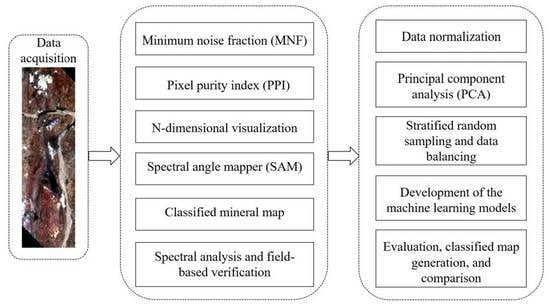
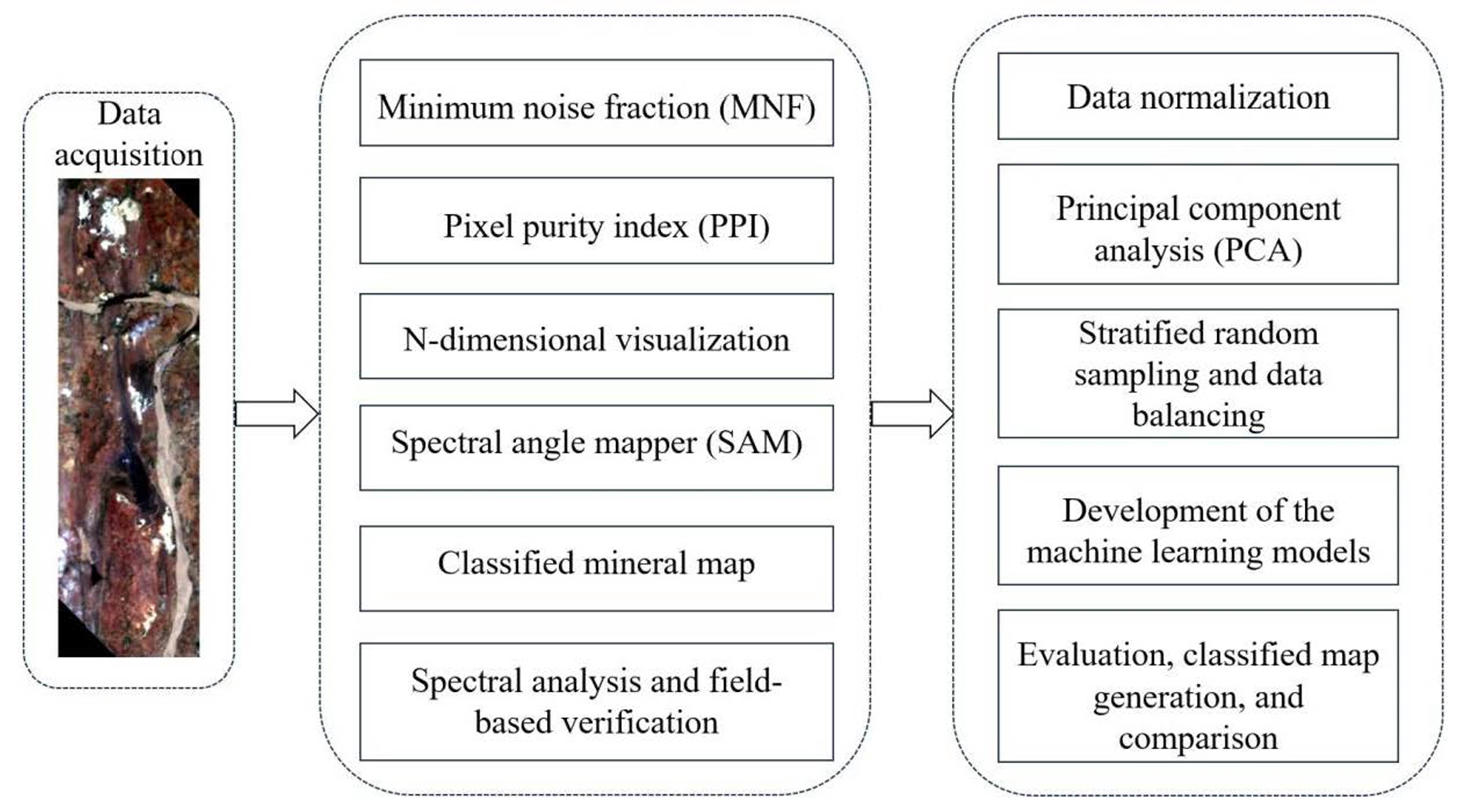
4. Materials and Methods

The workflow in Figure 2 depicts the steps followed to MPM. The supervised MLAs require training and test pixels, which are obtained through a ground-verified reference mineral distribution map. Therefore, initially SAM, minimum noise fraction (MNF) [27], pixel purity index (PPI) [28], and N-dimensional visualization [29] techniques were used to generate the reference mineral distribution map. In the next step, the generated mineral distribution map was extensively validated with field verification. In the third stage, ML-based predictive models were developed. In the fourth stage, the performance of the developed models was verified using various evaluation measures, and classified mineral maps were generated.

4.1. Generation of the Reference Mineral Distribution Map

The techniques of SAM, MNF, PPI, and N-Dimensional visualization have been used to prepare the reference map, which was verified during the extensive field-survey. The MNF technique maximizes separability between mineral classes and minimizes noise in the captured image. Pure pixels in images were identified and extracted using PPI and N-dimensional visualization techniques, which were used to generate the mineral map. Figure 3 shows the classified reference map with the corresponding RGB image of the scene. In the classified image, red, green, and yellow pixels represent the existence of kaolinite, talc, and montmorillonite mineral, respectively. In the end, the prepared dataset contained 120 pixels of kaolinite, 383 pixels of talc, 35 pixels of montmorillonite minerals; and 173 spectral features or bands.

4.2. Field-Based Verification

To validate the obtained map, a field-survey has been performed in the marked area of the RGB PRISMA image. Five significant surface exposures of altered/weathered mineral mines have been identified in the study area—the Gheoriya talc mine, adjacent to the Gheoriya talc mine, the Ampura kaolinite mine, the Madhopur talc mine, and the Abhaipur mine (marked as A, B, C, D, E, respectively, in Figure 3).

4.3. Development of ML-Based Predictive Models

4.3.1. Data Normalization

The normalization techniques are used to rescale the values in the dataset to a standard range so as to allow equal contribution of all features presented by the data for the learning algorithms. There are various techniques for data normalization, such as min-max normalization, log scaling, decimal scaling, Z-score normalization, etc. In this study, the Z-score normalization technique has been used to rescale the spectral features of the pixels, which is represented as Equation (1) [30].
X = X X ¯ SD
where  X  denotes the spectral feature vector, and  X ¯  and  SD  are the mean and standard deviation of  X , respectively. The value  X = 0  indicates a spectral feature similar to the mean value, and  | X | = ± n  indicates n SD units distant (above or below) spectral feature from the mean.

4.3.2. Principal Component Analysis

To reduce the spectral dimension, the feature extraction technique of PCA has been used. The technique finds orthogonal projections of the dataset to construct an uncorrelated set of principal components (PCs). In the case of HSI, if  H R n × d  represents the spectral reflectance matrix of  n  pixels of each  d  dimension, then the vector  [ x i 1 , x i 2 , , x i d ]  corresponds to the  i t h  pixel. The PCA technique can be performed on spectral reflectance matrix  H  (Equation (2)) to reduce the dimension  d  of these  n  pixels [31].
H ( n × d ) = [ x 11 x 1 j x 1 d x i 1 x i j x i d x n 1 x n j x n d ]
The covariance matrix  C ( d × d )  obtained from matrix  H  is decomposed to obtain eigenvalues and eigenvectors as in Equation (3).
C ( d × d ) = E λ E T
where  λ  denotes the matrix of the eigenvalues and  E  represents the matrix of the eigenvectors. The variance concerning PCs is determined by the eigenvalues; therefore, the eigenvectors  E  are arranged based on the values of  λ . Furthermore, the projected matrix is obtained using Equation (4).
Z ( n × d ) = H ( n × d ) E ( d × d )
The initial columns of projected matrix  Z  contain PCs which pose maximal variance and minimal correlation.

4.3.3. Development and Evaluation of ML-Based Mapping Models

Machine learning (ML) facilitates dynamic modeling capable of learning hidden patterns associated with provided data (training data) to produce predictions about unseen data without being explicitly programmed. Since these techniques provide automated predictions for unseen datasets, they are prevalent in remote-sensing-based research domains [10]. To classify the selected minerals, the present study employs various supervised ML-based algorithms, namely SVM, DT, tree bagging, RF, extremely randomized trees (ET), ANN, KNN, Gaussian process classification (GPC), Ada Boost, gradient boosting classifier (GBC), extreme gradient boosting (XGBoost), light gradient boosting machine (LGBM), category boosting (CATBoost), histogram gradient boosting (HGB), stochastic gradient descent (SGD), Gaussian naïve bayes (GNB), LDA, and quadratic discriminant analysis (QDA).
The SVM classifier uses statistical theory to find a separating hyperplane or decision boundary to classify the samples [32]. It was initially developed for binary classification, but later multiclass classification was performed through its repeated applications. The multiclass classification with the SVM classifier can be performed with either a ‘one-vs-one’ or ‘one-vs-rest’ strategy [33].
DT uses decision statements to construct the tree, such that the nodes represent decision rules, branches represent outcomes of decision rules, and the leaf nodes represent class labels [34]. The DT can be constructed with iterative dichotomizer 3 (ID3), C 4.5, and classification and regression tree (CART) algorithms. The bagging classifier constructs multiple learners based on the bootstrapping of samples (with all features) and combines them through aggregation. The bootstrap samples are generated through random selection with a replacement strategy. The RF model constructs multiple DTs and combines the predictions through majority voting to obtain the final predictions [35]. It uses two basic principles during the training process: random feature subset selection and bootstrap aggregation (bagging) [36]. Similar to the RF model, the ET classifier is also an ensemble-based approach that constructs multiple DTs and makes the predictions through combination [37]. It has two key differences from RF: first, instead of bootstrap samples, it uses the entire dataset to train each DT. Second, it is based on random splits of features rather than best splits.
ANN attempts to imitate the workings of the human brain. Similar to the human brain, it consists of a collection of connected artificial neurons or nodes in various layers [38]. Activation function, topology, inputs, and connection weights are the most prevalent factors that define ANN. The KNN classifier assumes the distance measure of the selected sample to the available samples, and classifies it to the category of k-nearest-neighbor samples [39]. The most common measures include Manhattan distance (city block), Euclidean distance (Frobenius), and Minkowsky distance. GPC assumes a two-stage classification model to estimate class probabilities [40]. It requires specifying a kernel function or nuisance function to measure the covariance of the data. Then, the link function computes the class membership probabilities.
Ada Boost classifier is an iterative ensemble model based on a boosting technique that constructs a robust classifier by improving the classification performance of a weak learner in the previous iteration through increasing weights of misclassified samples [41]. GBC is also based on a boosting technique, but instead of re-weighting the samples, it fits the learner to the residual error of the previous iteration determined using the gradient descent technique [42]. XGBoost [43], LGBM [44], CATBoost [45], and HGB are the variants of GBC, which are designed for larger datasets and distributed computing. XGBoost poses a regularization ability to avoid overfitting. LGBM requires lower memory for execution and is faster than GBC. It is based on the leaf-growing strategy; therefore, it efficiently prevents overfitting. The algorithm introduces two techniques into traditional GBC: “gradient-based one-side sampling (GOSS)” and “exclusive feature bundling (EFB)”. CATBoost can efficiently deal with categorical features with minimum information loss during training. It uses the concept of ordered boosting to overcome the target leakage issue in GBC. HGB constructs a histogram of feature values through division of continuous variables into bins, and uses those bins instead of feature values for splitting. Therefore, it reduces searching time for optimal splits.
The SGD classifier uses an iterative stochastic gradient descent method for computing loss functions and penalties during classification [46]. GNB is a probabilistic classification technique that applies the “Bayes theorem”. It assumes feature independence and equal contribution toward probability estimates for belongingness to a specific class [47]. Discriminant analysis, i.e., LDA and QDA, are probability-based classification techniques that aim to separate the feature space through the minimization of within-class variance and maximization of between-class variance [48,49]. According to their names, LDA generates linear decision boundaries, whereas QDA generates quadratic decision boundaries. The difference among them is that first, the LDA is used for linear classification, whereas QDA is used for non-linear classification as it generates quadratic decision boundaries. Second, LDA computes a single covariance matrix for all classes, whereas QDA computes multiple covariance matrices for each class; thus, it is computationally expensive and flexible compared to LDA. Third, LDA works better with smaller datasets, while QDA works better with larger datasets.
Figure 4 shows the development and evaluation process of ML-based classification models. The labeled dataset is required during the learning phase of supervised classifiers; therefore, the initial seventeen principal components and the SAM-classified mineral distribution map were used to create the spectral dataset and develop the predictive models. For splitting the pixels of the prepared dataset into training and test sets, the stratified random sampling (SRS) technique was adopted. The SRS involves dividing the sample pixels into strata or subgroups based on the relevant characteristic such as class labels. The samples are drawn randomly from each stratum according to the defined proportions.
Furthermore, the synthetic minority oversampling technique (SMOTE) was performed over the training set to eliminate its imbalance [50]. The SMOTE technique synthesizes new samples from the minority class samples. The SMOTE technique works in the following way: initially, a minority class sample is chosen. Then, its k-nearest samples are found, and one of them is selected randomly for computation. The difference between the selected sample and its randomly selected neighborhood is evaluated. The obtained difference is multiplied by a random number and added to the minority sample under consideration to obtain a synthetic sample. This approach forces it to create a convex combination of the minority class sample and its k-nearest neighbor sample. Finally, the hyperparameters of the models were tuned to train the models using pixels of the training set. In the evaluation phase, pixels of the test set were used.

5. Performance Measures

To evaluate the performance of the developed classification models, various measures have been used, such as the average accuracy (AA), overall accuracy (OA), recall, precision, F1-score, kappa coefficient (k), and receiver operating characteristic (ROC) curve. Average accuracy corresponds to the average accuracy for each mineral class, i.e., the average of the ratio of numbers of accurately classified pixels to the total pixels of a mineral class. Overall accuracy corresponds to the ratio between accurately classified pixels and the number of pixels in the dataset. The recall value demonstrates the classifier’s capacity to make accurate predictions for positive classes. The precision value reflects the ability of a classifier to make positive predictions among all positive predictions. The harmonic mean of recall and precision is the F1-score. The kappa coefficient is the measure of agreement between different predictions. Its value ranges between 0–1. The ROC curve facilitates the visualization of the diagnostic capability of the classifier at different thresholds of true positive rate (TPR) and false positive rate (FPR). The AUC (area under the ROC curve) score indicates the capability of the classifier to distinguish between different class samples. A higher AUC score indicates better performance. The mathematical equations for these measures are listed in Table 2. In these equations, the terms  t p i t n i f p i , and  f n i  represent true positive, true negative, false positive, and false negative, respectively; and  c  represent mineral class. The present mineral classification is a three-class classification problem; therefore, for computing these terms, the pixels belonging to a specific mineral class are considered as positive, and the rest as negative.

6. Results and Discussion

This section explores the results obtained during the study, spectral analysis, and predictive capabilities of the ML techniques.

6.1. Spectral Absorption Characteristics of the Minerals

As mentioned in Section 4.2, to validate the generated SAM based mineral distribution map, an extensive field survey has been performed. In the study area, five main surface exposures of the altered/weathered minerals have been observed. Figure 5a (marked as A in Figure 3) depicts the exposure of talc mineral observed at the Gheoriya mining area, and the spectral absorption region was found at 2.315 µm in the corresponding spectral signature, which meets the absorption characteristic of the mineral. Figure 5b (marked as B in Figure 3) depicts the area adjacent to the Gheoriya mining location. The spectral plot of the image and USGS spectra also confirms the dominance of a mixture of Montmorillonite minerals in this location. The spectral absorption region was found at 2.205 µm in the corresponding spectral signature, which meets the absorption characteristic of the mineral. Figure 5c (marked as C in Figure 3) depicts the surface exposure of kaolinite mineral at the Ampura mining area and its spectral plot. The spectral plot between the image and USGS spectra confirms a doublet of absorption feature at 2.165 µm and 2.205 µm, which meets the absorption characteristic of the mineral. Similarly, Figure 5d,e (marked as D and E in Figure 3) depicts the surface exposures of talc minerals at the Madhopur and Abhaipur areas, and their corresponding spectral absorption region at 2.315 µm. The spectral plot for this area also confirms the occurrence of this mineral.

6.2. Dimensionality Reduction

As mentioned in Section 4.3.1, the ‘Z-normalization’ technique has been adopted to normalize the prepared spectral dataset. The correlation matrix plot corresponding to the normalized dataset of 171 spectral features is represented in Figure 6a. It can be observed from the plot that the correlation coefficient between the spectral features ranges between −0.3713 to 1. Furthermore, the spectral features 40–50, 84–100, and 166–171 are less correlated to other features, while the rest are highly correlated. The high correlation among the spectral features and the large dimensionality results in complex and costlier model formulation. Therefore, to retain significant information, the feature reduction technique of PCA has been employed. It is evident from the variance plot in Figure 6b that the initial 17 principal components retain 95% of the total variance; therefore, these are employed for classification model development. Figure 7 shows the 3D scatter plot for the first three principal components. It is evident that the ‘Talc’ mineral shows liner separation, while the other two minerals depict non-linear separation. Therefore, linear and non-linear methods of ML classification algorithms were employed in the study.

6.3. Balancing of the Training Dataset

The distribution of the pixels is depicted in Table 3. These pixels are distributed into training and test sets using a stratified random sampling approach. To investigate the sensitivity of the ML models in terms of split size, the split ratio of 30:70, 50:50, and 70:30 have been tested in the study. An imbalanced training set can result in biased classification results. Therefore, the oversampling technique of ‘SMOTE’ has been applied to the training set.

6.4. Hyper-Parameter Optimization of the Classification Models

There are two types of parameters associated with the ML models: ‘model parameters’ and ‘hyper-parameters’. The ‘model parameters’ are configured during the training phase, whereas hyper-parameters are pre-configured manually before the training phase. Furthermore, the appropriate selection of hyperparameters is imperative for the optimal performance of the model. The present study uses a grid search with a five-fold cross-validation technique to optimize the hyperparameters of the models. In this technique, the candidate parameter values are exhaustively generated and evaluated from all the combination of specified ranges. The important parameters of different MLAs which are optimized using this technique are represented in Table 4.

6.5. Comparison of Classification Models

This subsection describes the evaluated outcomes of the classification algorithms for different split ratios. The five-fold cross-validation technique was used to train the classification models, and the evaluation of the developed models was performed using the test dataset.

6.5.1. Results Obtained with the 30:70 Split

Table 5 illustrates the evaluated performance measures using the confusion matrix in Figure A2 of Appendix A and the measures listed in Table 2. It can be observed from Table 5 that for the 30:70 split ratio of the dataset, the SGD classifier outperformed all the classifiers and achieved the scores of OA—99.2%, AA—97.87%, K—0.9819, F1-score—98.14%, and Recall—97.87%. In terms of OA, AA, K, F1-score, and Recall measures, QDA performed lowest among all, with scores of 89.92%, 62.44%, 0.7436, and 62.82%, respectively. However, in terms of precision score, GPC achieved the lowest score of 83.10%. The classified maps are shown in Figure A1 of Appendix A. The SGT classifier is very much closer to the reference mineral distribution map (Figure 3). If compared in terms of individual class accuracies (Table 6) for ‘Montmorillonite’ mineral, the GBC and LGBM classifiers achieved the highest accuracy. The QDA classifier misclassified significant instances of pixels belonging to ‘Montmorillonite’ with the lowest accuracy of 4%. For the ‘Talc’ mineral, all the classifiers achieved higher accuracies except for the HGB classifier, which achieved 97% accuracy. Due to the smaller number of reference pixels belonging to the ‘Kaolinite’ mineral, all the models were underfitted and depict less accuracy. Among all the classifiers, the SGD classifier achieved the highest accuracy of 98% for the ‘Kaolinite’ mineral. For ‘Kaolinite’, DT is the most diminutive performer with an accuracy score of 68%. It can be observed from the ROC curves in Figure A3 of Appendix A that LDA, GNB, SGD, LGBM, XGB, HGB, and ET show the highest mean AUC score of 1, while QDA and DT were worst performers in terms of AUC score, which achieved scores of 0.84 and 0.87, respectively.

6.5.2. Results Obtained with the 50:50 Split

Table 7 illustrates the evaluated results using the confusion matrix (Figure A5 of Appendix B). It can be observed from the listed results that for the 50:50 split of the dataset, the ANN-based MLP classifier and SGD classifier outperformed all the classifiers and achieved a score of 100% for all the measures. The AdaBoost classifier is the lowest performer in terms of all the measures. The classified maps are represented in Figure A4 of Appendix B. In terms of accuracies for each class (Table 8), k-NN, AdaBoost, GBC, XGB, LGBM, SGD, and MLP are the most accurate in predictions of ‘Montmorillonite’ occurrences. In contrast, QDA is the worst performer in predicting this mineral, with an accuracy score of 22%. All the classifiers achieved higher accuracies for the ‘Talc’ mineral due to a larger number of reference pixels. For ‘Kaolinite’, RF, ET, SGD, and MLP achieved the highest accuracy, while AdaBoost encountered failures in predicting the mineral. It can be observed from the ROC curves in Figure A6 of Appendix B that MLP, LDA, GNB, SGD, HGB, CATBoost, LGBM, XGB, GBC, GPC, k-NN, ET, RF, Bagging Classifier, and SVM achieved the highest mean AUC score of 1, while QDA, AdaBoost, and DT were the worst performers in terms of AUC score, and achieved scores of 0.87, 0.94, and 0.97, respectively.

6.5.3. Results Obtained with the 70:30 Split

Table 9 illustrates the evaluated performance measures using the confusion matrix in Figure A8 of Appendix C and the measures listed in Table 2. It can be observed from Table 2 that for the 70:30 split of the dataset, the MLP classifier outperformed all the classifiers and achieved a score of 100% concerning all the measures. As in the 50:50 split, the AdaBoost classifier is the lowest performer in all the measures. The classified maps are represented in Figure A7 of Appendix C. In terms of each class accuracy (Table 10), SVM, k-NN, GPC, AdaBoost, GBC, XGB, LGBM, HGB, and MLP are the most accurate in predictions of ‘Montmorillonite’ occurrences. However, as with the 50:50 split, QDA is the worst performer in predicting this mineral, with an accuracy score of 36%. As with the previous splits for the ‘Talc’ mineral, all the classifiers achieved higher accuracies. For ‘Kaolinite’, ET, SGD, and MLP achieved the highest accuracy, while AdaBoost encountered failures in predicting the mineral. It can be observed from the ROC curves in Figure A9 of Appendix C that MLP, LDA, GNB, SGD, HGB, CATBoost, LGBM, XGB, GBC, GPC, ET, RF, Bagging Classifier, and SVM achieved the highest mean AUC score of 1, while QDA, AdaBoost, and DT were the worst performers in terms of AUC score, and achieved scores of 0.98, 0.94, and 0.94, respectively.
Overall, the results from the experiments infer that the SGD classifier outperformed for the smaller and moderate training set (30:70 and 50:50 split ratio), while the MLP classifier outperformed for the moderate and larger training set (50:50 and 70:30 split ratio). All the classifiers achieved higher classification scores for the ‘Talc’ mineral due to the large number of samples. The QDA and AdaBoost classifiers were the least performers amongst all due to small sample size.

7. Conclusions

This study explored and evaluated the ability of the PRISMA SWIR sensor to map hydrothermally altered and weathered minerals using various machine learning algorithms. The significant findings of the proposed study are as follows.
  • The low SNR of the PRISMA dataset does not seem to affect its ability to classify the altered minerals using ML techniques.
  • The spectral information associated with the SWIR bands of the PRISMA dataset is sufficient to discriminate the selected minerals.
  • The stochastic gradient descent and artificial-neural-network-based multilayer perceptron algorithms are the most efficient ML techniques for the classification of specified mineral using the PRISMA dataset.
  • The linear feature transformation technique of PCA can efficiently derive crucial information to map the selected minerals.
The results confirm the machine-learning-based mineral classification attempt using the PRISMA hyperspectral image as a promising approach. The study can be extended to investigate the novel techniques for this new hyperspectral sensor; for instance, feature extraction, band selection, object-based classification, target detection, and pan-sharpening techniques.

Author Contributions

Methodology, investigation, software, writing—original draft preparation, N.A.; conceptualization, formal analysis, supervision, writing—review and editing, H.G., M.G. and P.K.S.; validation, resources, G.M. All authors have read and agreed to the published version of the manuscript.

Funding

This research received no external funding.

Data Availability Statement

Not applicable.

Conflicts of Interest

The authors declare no conflict of interest.

Appendix A. Results Obtained with 30:70 Spit Ratio

Figure A1. Classified images generated by (a) SVM (b) DT (c) Bagging Classifier (d) RF (e) ET (f) KNN (g) GPC (h) Ada Boost (i) GBC (j) XGB (k) LGBM (l) Cat Boost (m) HGB (n) SGD (o) GNB (p) LDA (q) QDA (r) MLP Classifier.
Remotesensing 15 03133 g0a1
Figure A2. Confusion matrix for classified pixels using (a) SVM (b) DT (c) Bagging Classifier (d) RF (e) ET (f) KNN (g) GPC (h) Ada Boost (i) GBC (j) XGB (k) LGBM (l) Cat Boost (m) HGB (n) SGD (o) GNB (p) LDA (q) QDA (r) MLP Classifier.
Remotesensing 15 03133 g0a2
Figure A3. ROC curves generated by (a) SVM (b) DT (c) Bagging Classifier (d) RF (e) ET (f) KNN (g) GPC (h) Ada Boost (i) GBC (j) XGB (k) LGBM (l) Cat Boost (m) HGB (n) SGD (o) GNB (p) LDA (q) QDA (r) MLP Classifier.
Remotesensing 15 03133 g0a3aRemotesensing 15 03133 g0a3bRemotesensing 15 03133 g0a3c

Appendix B. Results Obtained with 50:50 Spit Ratio

Figure A4. Classified images generated by (a) SVM (b) DT (c) Bagging Classifier (d) RF (e) ET (f) KNN (g) GPC (h) Ada Boost (i) GBC (j) XGB (k) LGBM (l) Cat Boost (m) HGB (n) SGD (o) GNB (p) LDA (q) QDA (r) MLP Classifier.
Remotesensing 15 03133 g0a4
Figure A5. Confusion matrix for classified pixels using (a) SVM (b) DT (c) Bagging Classifier (d) RF (e) ET (f) KNN (g) GPC (h) Ada Boost (i) GBC (j) XGB (k) LGBM (l) Cat Boost (m) HGB (n) SGD (o) GNB (p) LDA (q) QDA (r) MLP Classifier.
Remotesensing 15 03133 g0a5
Figure A6. ROC curves generated by (a) SVM (b) DT (c) Bagging Classifier (d) RF (e) ET (f) KNN (g) GPC (h) Ada Boost (i) GBC (j) XGB (k) LGBM (l) Cat Boost (m) HGB (n) SGD (o) GNB (p) LDA (q) QDA (r) MLP Classifier.
Remotesensing 15 03133 g0a6aRemotesensing 15 03133 g0a6bRemotesensing 15 03133 g0a6c

Appendix C. Results Obtained with 70:30 Spit Ratio

Figure A7. Classified images generated by (a) SVM (b) DT (c) Bagging Classifier (d) RF (e) ET (f) KNN (g) GPC (h) Ada Boost (i) GBC (j) XGB (k) LGBM (l) Cat Boost (m) HGB (n) SGD (o) GNB (p) LDA (q) QDA (r) MLP Classifier.
Remotesensing 15 03133 g0a7
Figure A8. Confusion matrix for classified pixels using (a) SVM (b) DT (c) Bagging Classifier (d) RF (e) ET (f) KNN (g) GPC (h) Ada Boost (i) GBC (j) XGB (k) LGBM (l) Cat Boost (m) HGB (n) SGD (o) GNB (p) LDA (q) QDA (r) MLP Classifier.
Remotesensing 15 03133 g0a8
Figure A9. ROC curves generated by (a) SVM (b) DT (c) Bagging Classifier (d) RF (e) ET (f) KNN (g) GPC (h) Ada Boost (i) GBC (j) XGB (k) LGBM (l) Cat Boost (m) HGB (n) SGD (o) GNB (p) LDA (q) QDA (r) MLP Classifier.
Remotesensing 15 03133 g0a9aRemotesensing 15 03133 g0a9bRemotesensing 15 03133 g0a9c

References

  1. Ghamisi, P.; Plaza, J.; Chen, Y.; Li, J.; Plaza, A.J. Advanced Spectral Classifiers for Hyperspectral Images: A Review. IEEE Geosci. Remote Sens. Mag. 2017, 5, 8–32. [Google Scholar] [CrossRef] [Green Version]
  2. Mishra, G.; Govil, H.; Srivastava, P.K. Identification of Malachite and Alteration Minerals Using Airborne AVIRIS-NG Hyperspectral Data. Quat. Sci. Adv. 2021, 4, 100036. [Google Scholar] [CrossRef]
  3. Abdelsalam, M.G.; Stern, R.J.; Berhane, W.G. Mapping Gossans in Arid Regions with Landsat TM and SIR-C Images: The Beddaho Alteration Zone in Northern Eritrea. J. Afr. Earth Sci. 2000, 30, 903–916. [Google Scholar] [CrossRef]
  4. Qian, S.-E. Hyperspectral Satellites, Evolution, and Development History. IEEE J. Sel. Top. Appl. Earth Obs. Remote Sens. 2021, 14, 7032–7056. [Google Scholar] [CrossRef]
  5. Cogliati, S.; Sarti, F.; Chiarantini, L.; Cosi, M.; Lorusso, R.; Lopinto, E.; Miglietta, F.; Genesio, L.; Guanter, L.; Damm, A.; et al. The PRISMA Imaging Spectroscopy Mission: Overview and First Performance Analysis. Remote Sens. Environ. 2021, 262, 112499. [Google Scholar] [CrossRef]
  6. Loizzo, R.; Daraio, M.; Guarini, R.; Longo, F.; Lorusso, R.; Dini, L.; Lopinto, E. Prisma Mission Status and Perspective. In Proceedings of the IGARSS 2019—2019 IEEE International Geoscience and Remote Sensing Symposium, Yokohama, Japan, 28 July–2 August; pp. 4503–4506.
  7. Zuo, R. Machine Learning of Mineralization-Related Geochemical Anomalies: A Review of Potential Methods. Nat. Resour. Res. 2017, 26, 457–464. [Google Scholar] [CrossRef]
  8. Ghamisi, P.; Yokoya, N.; Li, J.; Liao, W.; Liu, S.; Plaza, J.; Rasti, B.; Plaza, A. Advances in Hyperspectral Image and Signal Processing: A Comprehensive Overview of the State of the Art. IEEE Geosci. Remote Sens. Mag. 2017, 5, 37–78. [Google Scholar] [CrossRef] [Green Version]
  9. McCoy, J.T.; Auret, L. Machine Learning Applications in Minerals Processing: A Review. Miner. Eng. 2019, 132, 95–109. [Google Scholar] [CrossRef]
  10. Maxwell, A.E.; Warner, T.A.; Fang, F. Implementation of Machine-Learning Classification in Remote Sensing: An Applied Review. Int. J. Remote Sens. 2018, 39, 2784–2817. [Google Scholar] [CrossRef] [Green Version]
  11. Tuşa, L.; Kern, M.; Khodadadzadeh, M.; Blannin, R.; Gloaguen, R.; Gutzmer, J. Evaluating the Performance of Hyperspectral Short-Wave Infrared Sensors for the Pre-Sorting of Complex Ores Using Machine Learning Methods. Miner. Eng. 2020, 146, 106150. [Google Scholar] [CrossRef]
  12. Kumar, C.; Chatterjee, S.; Oommen, T.; Guha, A. Automated Lithological Mapping by Integrating Spectral Enhancement Techniques and Machine Learning Algorithms Using AVIRIS-NG Hyperspectral Data in Gold-Bearing Granite-Greenstone Rocks in Hutti, India. Int. J. Appl. Earth Obs. Geoinf. 2020, 86, 102006. [Google Scholar] [CrossRef]
  13. Lorenz, S.; Ghamisi, P.; Kirsch, M.; Jackisch, R.; Rasti, B.; Gloaguen, R. Feature Extraction for Hyperspectral Mineral Domain Mapping: A Test of Conventional and Innovative Methods. Remote Sens. Environ. 2021, 252, 112129. [Google Scholar] [CrossRef]
  14. Parakh, K.; Thakur, S.; Chudasama, B.; Tirodkar, S.; Porwal, A.; Bhattacharya, A. Machine Learning and Spectral Techniques for Lithological Classification. In Proceedings of the Multispectral, Hyperspectral, and Ultraspectral Remote Sensing Technology, Techniques and Applications VI, New Delhi, India, 4–7 April 2016; SPIE: Bellingham, WA, USA, 2016; Volume 9880, pp. 456–467. [Google Scholar]
  15. Pal, M.; Rasmussen, T.; Porwal, A. Optimized Lithological Mapping from Multispectral and Hyperspectral Remote Sensing Images Using Fused Multi-Classifiers. Remote Sens. 2020, 12, 177. [Google Scholar] [CrossRef] [Green Version]
  16. Lobo, A.; Garcia, E.; Barroso, G.; Martí, D.; Fernandez-Turiel, J.-L.; Ibáñez-Insa, J. Machine Learning for Mineral Identification and Ore Estimation from Hyperspectral Imagery in Tin–Tungsten Deposits: Simulation under Indoor Conditions. Remote Sens. 2021, 13, 3258. [Google Scholar] [CrossRef]
  17. Eichstaedt, H.; Ho, C.Y.J.; Kutzke, A.; Kahnt, R. Performance Measurements of Machine Learning and Different Neural Network Designs for Prediction of Geochemical Properties Based on Hyperspectral Core Scans. Aust. J. Earth Sci. 2022, 69, 733–741. [Google Scholar] [CrossRef]
  18. Shirmard, H.; Farahbakhsh, E.; Heidari, E.; Beiranvand Pour, A.; Pradhan, B.; Müller, D.; Chandra, R. A Comparative Study of Convolutional Neural Networks and Conventional Machine Learning Models for Lithological Mapping Using Remote Sensing Data. Remote Sens. 2022, 14, 819. [Google Scholar] [CrossRef]
  19. Shayeganpour, S.; Tangestani, M.H.; Gorsevski, P.V. Machine Learning and Multi-Sensor Data Fusion for Mapping Lithology: A Case Study of Kowli-Kosh Area, SW Iran. Adv. Space Res. 2021, 68, 3992–4015. [Google Scholar] [CrossRef]
  20. Yousefi, B.; Sojasi, S.; Castanedo, C.I.; Maldague, X.P.V.; Beaudoin, G.; Chamberland, M. Comparison Assessment of Low Rank Sparse-PCA Based-Clustering/Classification for Automatic Mineral Identification in Long Wave Infrared Hyperspectral Imagery. Infrared Phys. Technol. 2018, 93, 103–111. [Google Scholar] [CrossRef]
  21. Lin, N.; Chen, Y.; Liu, H.; Liu, H. A Comparative Study of Machine Learning Models with Hyperparameter Optimization Algorithm for Mapping Mineral Prospectivity. Minerals 2021, 11, 159. [Google Scholar] [CrossRef]
  22. Guo, X.; Li, P.; Li, J. Lithological Mapping Using EO-1 Hyperion Hyperspectral Data and Semisupervised Self-Learning Method. J. Appl. Remote Sens. 2021, 15, 032209. [Google Scholar] [CrossRef]
  23. Malhotra, G.; Pandit, M.K. Geology and Mineralization of the Jahazpur Belt, Southeastern Rajasthan. In Crustal Evolution and Metallogeny in the Northwestern Indian Shield: A Festschrift for Asoke Mookherjee; Alpha Science International: Oxford, UK, 2000; pp. 115–125. [Google Scholar]
  24. Roy, A.B.; Jakhar, S.R. Geology of Rajasthan (Northwest India): Precambrian to Recent; Scientific Publishers: Jodhpur, India, 2002; ISBN 978-81-7233-304-1. [Google Scholar]
  25. Tripathi, M.K.; Govil, H. Regolith Mapping and Geochemistry of Hydrothermally Altered, Weathered and Clay Minerals, Western Jahajpur Belt, Bhilwara, India. Geocarto International. 2022, 37, 879–895. [Google Scholar] [CrossRef]
  26. Pandit, M.K.; Sial, A.N.; Malhotra, G.; Shekhawat, L.S.; Ferreira, V.P. C-, O- Isotope and Whole-Rock Geochemistry of Proterozoic Jahazpur Carbonates, NW Indian Craton. Gondwana Res. 2003, 6, 513–522. [Google Scholar] [CrossRef]
  27. Green, A.A.; Berman, M.; Switzer, P.; Craig, M.D. A Transformation for Ordering Multispectral Data in Terms of Image Quality with Implications for Noise Removal. IEEE Trans. Geosci. Remote Sens. 1988, 26, 65–74. [Google Scholar] [CrossRef] [Green Version]
  28. Boardmann, J.; Kruse, F.A.; Green, R.O. Mapping Target Signatures via Partial Unmixing of AVIRIS Data. In Proceedings of the Summaries of the 5th Annual JPL Airborne Geoscience Workshop, Pasadena, CA, USA, 23–26 January 1995; Volume 1, pp. 95–101. [Google Scholar]
  29. Kruse, F.A.; Richardson, L.L.; Ambrosia, V.G. Techniques Developed for Geologic Analysis of Hyperspectral Data Applied to Near-Shore Hyperspectral Ocean Data. In Proceedings of the Fourth International Conference on Remote Sensing for Marine and Coastal Environments: Environmental Research Institute of Michigan (ERIM), Orlando, FL, USA, 17–19 March 1997. [Google Scholar]
  30. Singh, D.; Singh, B. Investigating the Impact of Data Normalization on Classification Performance. Appl. Soft Comput. 2020, 97, 105524. [Google Scholar] [CrossRef]
  31. Hotelling, H. Analysis of a Complex of Statistical Variables into Principal Components. J. Educ. Psychol. 1933, 24, 417–441. [Google Scholar] [CrossRef]
  32. Cortes, C.; Vapnik, V. Support Vector Machine. Mach. Learn. 1995, 20, 273–297. [Google Scholar] [CrossRef]
  33. Wang, Z.; Xue, X. Multi-Class Support Vector Machine. In Support Vector Machines Applications; Springer International Publishing: Cham, Switzerland, 2014; pp. 23–48. [Google Scholar]
  34. Quinlan, J.R. Simplifying Decision Trees. Int. J. Hum. Comput. Stud. 1999, 51, 497–510. [Google Scholar] [CrossRef] [Green Version]
  35. Breiman, L. Random Forests. Mach. Learn. 2001, 45, 5–32. [Google Scholar] [CrossRef] [Green Version]
  36. Liaw, A.; Wiener, M. Classification and Regression by RandomForest. R News 2002, 2, 18–22. [Google Scholar]
  37. Geurts, P.; Ernst, D.; Wehenkel, L. Extremely Randomized Trees. Mach. Learn. 2006, 63, 3–42. [Google Scholar] [CrossRef] [Green Version]
  38. Hykin, S. Neural Networks: A Comprehensive Foundation; Printice-Hall: Upper Saddle River, NJ, USA, 1999; pp. 120–134. [Google Scholar]
  39. Fix, E.; Hodges, J.L. Discriminatory Analysis. Nonparametric Discrimination: Consistency Properties. Int. Stat. Rev. Rev. Int. Stat. 1989, 57, 238. [Google Scholar] [CrossRef]
  40. Rasmussen, C.E. Gaussian Processes in Machine Learning; Springer: Berlin/Heidelberg, Germany, 2004; Volume 3176. [Google Scholar]
  41. Freund, Y.; Schapire, R.E. A Decision-Theoretic Generalization of on-Line Learning and an Application to Boosting. Lect. Notes Comput. Sci. Subser. Lect. Notes Artif. Intell. Lect. Notes Bioinforma. 1995, 904, 23–37. [Google Scholar] [CrossRef] [Green Version]
  42. Friedman, J.H. Greedy Function Approximation: A Gradient Boosting Machine. Ann. Stat. 2001, 29, 1189–1232. [Google Scholar] [CrossRef]
  43. Chen, T.; Guestrin, C. XGBoost: A Scalable Tree Boosting System. In Proceedings of the ACM SIGKDD International Conference on Knowledge Discovery and Data Mining, New York, NY, USA, 13–17 August 2016; pp. 785–794. [Google Scholar]
  44. Ke, G.; Meng, Q.; Finley, T.; Wang, T.; Chen, W.; Ma, W.; Ye, Q.; Liu, T.Y. LightGBM: A Highly Efficient Gradient Boosting Decision Tree. Adv. Neural Inf. Process. Syst. 2017, 30, 3147–3155. [Google Scholar]
  45. Prokhorenkova, L.; Gusev, G.; Vorobev, A.; Dorogush, A.V.; Gulin, A. Catboost: Unbiased Boosting with Categorical Features. Adv. Neural Inf. Process. Syst. 2018, 31, 6638–6648. [Google Scholar]
  46. Zhang, T. Solving Large Scale Linear Prediction Problems Using Stochastic Gradient Descent Algorithms. In Proceedings of the Twenty-First International Conference on Machine Learning, ICML 2004, New York, NY, USA, 4–8 July 2004; pp. 919–926. [Google Scholar]
  47. Murphy, K.P. Naive Bayes Classifiers. Univ. Br. Columbia 2006, 18, 1–8. [Google Scholar]
  48. Balakrishnama, S.; Ganapathiraju, A. Linear Discriminant Analysis—A Brief Tutorial. Compute 1998, 18, 1–8. [Google Scholar]
  49. Srivastava, S.; Gupta, M.R.; Frigyik, B.A. Bayesian Quadratic Discriminant Analysis. J. Mach. Learn. Res. 2007, 8, 1277–1305. [Google Scholar]
  50. Chawla, N.V.; Bowyer, K.W.; Hall, L.O.; Kegelmeyer, W.P. SMOTE: Synthetic Minority over-Sampling Technique. J. Artif. Intell. Res. 2002, 16, 321–357. [Google Scholar] [CrossRef]
Figure 1. Location map and lithological distribution of the study area [26].
Remotesensing 15 03133 g001
Figure 2. Flowgraph of the process.
Remotesensing 15 03133 g002
Figure 3. (a) PRISMA RGB imagery and (b) SAM classified mineral distribution map, where red, green, and yellow pixels represent the existence of kaolinite, talc, and montmorillonite, respectively.
Remotesensing 15 03133 g003
Figure 4. Development and evaluation of ML-based classification model.
Remotesensing 15 03133 g004
Figure 5. Field exposure of different minerals and their corresponding comparative spectral curves between image and USGS spectra, (a) shows absorption feature of talc at 2.315 µm with representative field image of talc surface exposure from Gheoriya, (b) represents absorption feature of montmorillonite at 2.205 µm from montmorillonite surface exposure adjacent to Gheoriya mining area, (c) shows doublet of absorption feature at 2.165 and 2.205 µm for kaolinite mineral from Ampura mine, (d,e) represents absorption feature for talc mineral at 2.315 µm from Abhaipur and Madhopur mining areas respectively.
Remotesensing 15 03133 g005aRemotesensing 15 03133 g005b
Figure 6. (a) Correlation coefficient matrix plot and (b) PCA variance plot.
Remotesensing 15 03133 g006
Figure 7. 3D scatter plot for the mineral distribution among the initial three PCs.
Remotesensing 15 03133 g007
Table 1. Specification of PRISMA dataset [5].
Orbit Altitude615 kmSpectral RangeVNIR—0.400–1.01 µm (66 bands)
SWIR—0.92–2.5 µm (173 bands)
PAN—0.4–0.7 µm
Swath Width30 kmSpectral Resolution≤12 nm
Field of View (FOV)2.77°Radiometric Resolution12 bits
Spatial ResolutionHyperspectral—30 m
Panchromatic—5 m
Signal-to-Noise Ratio (SNR)VNIR—>200:1
SWIR—>100:1
PAN—>240:1
Pixel SizeHyperspectral—30 µm × 30 µm
PAN—6.5 µm × 6.5 µm
Lifetime5 years
Table 2. Mathematical equation for the performance measures.
Measure Equation
Average Accuracy   1 c i = 1 c t p i + t n i t p i + t n i + f p i + f n i
Recall (TPR)   1 c i = 1 c t p i t p i + f n i
Precision   1 c i = 1 c t p i t p i + f p i
F1-score   2   ×   Precision   ×   Recall Precision   +   Recall
Kappa Coefficient   1 c i = 1 c 2 × ( t p i × t n i f p i + f n i ) ( t p i + f p i ) × ( t n i + f p i ) + ( t p i + f n i ) × ( t n i + f n i )
Table 3. Distribution of the pixels.
Class—IdMineral ClassTotal Pixels
1Montmorillonite 35
2Talc383
3Kaolinite and Kaosmec120
Table 4. Optimized parameters of the MLAs.
S. No.MLA NameOptimized Hyper ParametersRange
1SVMRegularization parameter or ‘C’[10−1–103]
‘kernel’[‘linear’, ‘poly’, ‘rbf’]
Kernel coefficient or ‘gamma’[10−3–1]
2DT‘criterion’[‘gini’, ‘entropy’]
‘max_depth’[1–10]
‘min_samples_split’[1–5]
‘max_features’[‘auto’, ‘sqrt’, ‘log2’]
3Bagging Classifier‘n_estimators’[1–30]
‘max_samples’[1–5]
4RF‘n_estimators’[1–30]
‘criterion’[‘gini’, ‘entropy’]
‘max_depth’[1–10]
‘min_samples_split’[1–5]
5ET‘n_estimators’[1–30]
‘criterion’[‘gini’, ‘entropy’]
‘max_depth’[1–10]
‘min_samples_split’[1–50]
6k-NN‘n_neighbors’[1–30]
7GPC ‘multi_class’[‘one_vs_rest’, ‘one_vs_one’]
8AdaBoost ‘n_estimators’[1–30]
9GBC‘n_estimators’ [1–30]
‘learning_rate’[0.01, 0.1, 1, 10]
10XGB‘max_depth’[1–10]
‘min_samples_split’ [1–50]
11LGBM ‘n_estimators’[1–30]
12Cat Boost‘max_depth’[1–10]
‘n_estimators’[1–30]
13HGB‘max_depth’[1–10]
14SGD‘penalty’[‘l2’, ‘l1’, ‘elasticnet’, None]
‘alpha’[0.0001, 0.001, 0.01, 0.1, 1, 10, 100, 1000]
15GNB‘var_smoothing’[1 × 10⁻⁶, 1 × 10⁻⁷, 1 × 10⁻⁸, 1 × 10⁻⁹, 1 × 10⁻¹⁰, 1 × 10⁻¹¹]
16LDA‘solver’[‘svd’, ‘lsqr’, ‘eigen’]
17QDA‘reg_param’[0–1]
18MLP‘hidden_layer_sizes’[(5,1), (5,2), (5,3), (10,1), (10,2), (10,3)]
‘activation’[‘tanh’, ‘relu’]
‘learning_rate’[‘constant’, ’adaptive’]
Table 5. Classification results achieved by different MLAs on the PRISMA dataset over test samples for 30:70 split.
MLA NameOAAAKF1-ScorePrecisionRecallAUC Score
1SVM0.96020.90850.91080.88440.86850.90850.99
2DT0.90720.82250.77950.81440.83830.82250.87
3Bagging Classifier0.91510.83440.79780.83480.85720.83440.97
4RF0.95230.89660.88830.91240.93060.89660.99
5ET0.96550.93900.92080.92310.91740.93901.00
6k-NN0.93630.87430.85710.84430.83480.87430.94
7GPC 0.93370.86100.85080.84310.83100.86100.95
8AdaBoost 0.94160.87680.86960.85270.83620.87680.99
9GBC0.93900.91690.86560.84810.84030.91690.98
10XGB 0.96290.93780.91660.90010.88310.93781.00
11LGBM 0.97350.96030.94040.92330.90480.96031.00
12Cat Boost 0.93630.87670.85040.86790.87930.87670.99
13HGB0.94160.92790.87190.88020.85060.92791.00
14SGD 0.99200.97870.98190.98010.98140.97871.00
15GNB0.94690.85510.87280.88930.93250.85511.00
16LDA0.95490.92320.89910.87580.86180.92321.00
17QDA0.89920.62440.74360.62820.92950.62440.84
18MLP 0.96020.90450.90970.90450.90450.90450.99
Table 6. Class accuracies achieved by different MLAs on the PRISMA dataset for test pixels (30:70 split ratio).
MLA NameMontmorilloniteTalcKaolinite
1SVM0.840.990.89
2DT0.800.990.68
3Bagging Classifier0.800.990.71
4RF0.840.990.86
5ET0.961.000.86
6k-NN0.800.980.85
7GPC 0.760.980.85
8AdaBoost 0.800.990.85
9GBC1.000.990.76
10XGB 0.961.000.86
11LGBM 1.001.000.88
12Cat Boost 0.881.000.75
13HGB0.960.970.86
14SGD 0.961.000.98
15GNB0.721.000.85
16LDA0.961.000.81
17QDA0.041.000.83
18MLP 0.800.990.93
Table 7. Classification results achieved by different MLAs on the PRISMA dataset over test samples for 50:50 split.
MLA NameOAAAKF1-ScorePrecisionRecallAUC Score
1SVM0.99260.97590.98320.97590.97590.97591.00
2DT0.97400.94810.94150.92280.90700.94810.97
3Bagging Classifier0.95910.92440.90710.92060.91740.92441.00
4RF0.99630.98150.99160.98770.99450.98151.00
5ET0.99260.96300.98310.97490.98920.96301.00
6k-NN0.97030.97080.93410.92980.90490.97081.00
7GPC 0.98510.96480.96640.95360.94430.96481.00
8AdaBoost 0.77320.66490.52350.45790.40950.66490.94
9GBC0.99630.99440.99160.98820.98250.99441.00
10XGB 0.98140.97220.95820.94490.92750.97221.00
11LGBM 0.98510.97780.96650.95520.93940.97781.00
12Cat Boost 0.98880.97040.97460.97220.97410.97041.00
13HGB0.98140.95930.95810.94300.93070.95931.00
14SGD 1.00001.00001.00001.00001.00001.00001.00
15GNB0.96650.88520.92110.92520.98080.88521.00
16LDA0.98140.95930.95810.94300.93070.95931.00
17QDA0.94050.72960.85990.75000.93840.72960.87
18MLP 1.00001.00001.00001.00001.00001.00001.00
Table 8. Class accuracies achieved by different MLAs on the PRISMA dataset for test pixels (50:50 split ratio).
MLA NameMontmorilloniteTalcKaolinite
1SVM0.941.000.98
2DT0.941.000.90
3Bagging Classifier0.890.980.90
4RF0.941.001.00
5ET0.891.001.00
6k-NN1.000.980.93
7GPC 0.941.000.95
8AdaBoost 1.000.990.00
9GBC1.001.000.98
10XGB 1.001.000.92
11LGBM 1.001.000.93
12Cat Boost 0.941.000.97
13HGB0.941.000.93
14SGD 1.001.001.00
15GNB0.721.000.93
16LDA0.941.000.93
17QDA0.221.000.97
18MLP 1.001.001.00
Table 9. Classification results achieved by different MLAs on the PRISMA dataset over test samples for the 70:30 split.
MLA NameOAAAKF1-ScorePrecisionRecallAUC Score
1SVM0.99380.99070.98610.98080.97220.99071.00
2DT0.96910.89690.92990.91240.93370.89690.94
3Bagging Classifier0.98150.95120.95820.94240.93490.95121.00
4RF0.98770.96040.97210.96040.96040.96041.00
5ET0.98770.93940.97200.95770.98250.93941.00
6k-NN0.96300.95720.91770.91430.89290.95720.99
7GPC 0.97530.96300.94360.94970.94300.96301.00
8AdaBoost 0.77160.66380.52060.45690.40840.66380.94
9GBC0.98770.98150.97220.96270.94870.98151.00
10XGB 0.97530.96300.94460.92910.91110.96301.00
11LGBM 0.99380.99070.98610.98080.97220.99071.00
12Cat Boost 0.97530.94190.94390.93600.93180.94191.00
13HGB0.99380.99070.98610.98080.97220.99071.00
14SGD 0.99380.96970.98600.97960.99100.96971.00
15GNB0.98150.93010.95730.95450.98500.93011.00
16LDA0.98770.96040.97210.96040.96040.96041.00
17QDA0.94440.76940.86970.80510.94150.76940.98
18MLP 1.00001.00001.00001.00001.00001.00001.00
Table 10. Class accuracies achieved by different MLAs on the PRISMA dataset for test pixels (70:30 split ratio).
MLA NameMontmorilloniteTalcKaolinite
1SVM1.001.000.97
2DT0.730.990.97
3Bagging Classifier0.911.000.94
4RF0.911.000.97
5ET0.821.001.00
6k-NN1.000.980.89
7GPC 1.001.000.89
8AdaBoost 1.000.990.00
9GBC1.001.000.94
10XGB 1.001.000.89
11LGBM 1.001.000.97
12Cat Boost 0.911.000.92
13HGB1.001.000.97
14SGD 0.911.001.00
15GNB0.821.000.97
16LDA0.911.000.97
17QDA0.361.000.94
18MLP 1.001.001.00
Disclaimer/Publisher’s Note: The statements, opinions and data contained in all publications are solely those of the individual author(s) and contributor(s) and not of MDPI and/or the editor(s). MDPI and/or the editor(s) disclaim responsibility for any injury to people or property resulting from any ideas, methods, instructions or products referred to in the content.

