
An Integrated Framework for Spatiotemporally Merging Multi-Sources Precipitation Based on F-SVD and ConvLSTM


Abstract
:
1. Introduction
2. Study Area and Materials
2.1. Study Area
2.2. Data
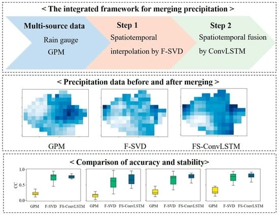
3. Methodology
3.1. F-SVD
- (1)
- The historical precipitation information from m surrounding gauges and n past moments needs to be prepared for the interpolation at the target point at a certain moment.
- (2)
- The precipitation data from the surrounding gauges and the target point from adjacent moments can form a spatiotemporal data matrix with dimensions of (m + 1) ×n, where the rows represent time and columns represent space.
- (3)
- If any precipitation values in the matrix representing the historical precipitation of the target point are unknown, traditional interpolation methods such as IDW should be used to calculate these values until only one null value representing the precipitation to be estimated remains.
- (4)
- The F-SVD method is utilized to decompose the matrix into a temporal feature matrix X and a spatial feature matrix Y. The stochastic gradient descent algorithm is used for optimization.
- (5)
- Then, the two optimal feature matrices are multiplied to reconstruct a matrix P, the element at the m + 1 row and n column in the reconstructed matrix represents the estimated precipitation, which is calculated as follows:
3.2. ConvLSTM
3.3. The Spatiotemporal Fusion Model
- (1)
- Download GPM satellite observation data with a spatial resolution of 0.1° and a temporal resolution of 0.5 h. Process the data to obtain precipitation data with a time interval of 1 h.
- (2)
- Collect and organize the rain gauge observation data of the study watershed and interpolate them into 0.1° × 0.1° spatial grid point data using the F-SVD method.
- (3)
- Construct input sample sets based on GPM and interpolation results of F-SVD, normalize the data, and use the data from 2006 to 2014 as the training set and the data from 2014 to 2018 as the testing set.
- (4)
- Train the model at 15 rain gauges with precipitation observations as the true value and mean squared error as the loss function to minimize the training loss.
- (5)
- Apply the trained model to each grid point within the study watershed for precipitation fusion.
3.4. Evaluation Indicators
4. Results
4.1. Quality Assessment of GPM
4.2. Accuracy Evaluation of Different Models
4.2.1. Accuracy Evaluation at Rain Gauges
4.2.2. Uncertainty Analysis
4.3. Model Performance in Typical Rainfall Events
4.3.1. Comparison of Temporal Variation Processes
4.3.2. Comparison of the Spatial Distribution
5. Discussion
6. Conclusions
- (1)
- The proposed FS-ConvLSTM framework outperforms the comparative models (IDW, F-SVD, and LSTM) in terms of precipitation variation process description and rainfall capture capability, reducing the RSME and FAR of the original GPM data by 63.6% and 63.1%, respectively, and increasing the CC and POD by 165% and 22.9%, respectively.
- (2)
- The merged data not only improve the accuracy of the precipitation but also reduce the uncertainty in precipitation estimation. As the intensity of precipitation increases, the precipitation capture ability substantially improves, and the estimation more closely matches the measured data in terms of total rainfall.
- (3)
- Due to the powerful feature extraction capability of ConvLSTM, the merged precipitation data combines the advantages of GPM and ground interpolation data with the continuous spatial distribution data and values close to the actual one, and the spatial aggregation of both data is reflected in the fusion.
Author Contributions
Funding
Data Availability Statement
Conflicts of Interest
References
- Hinge, G.; Hamouda, M.A.; Long, D.; Mohamed, M.M. Hydrologic utility of satellite precipitation products in flood prediction: A meta-data analysis and lessons learnt. J. Hydrol. 2022, 612, 128103. [Google Scholar] [CrossRef]
- Estébanez-Camarena, M.; Taormina, R.; van de Giesen, N.; ten Veldhuis, M.-C. The Potential of Deep Learning for Satellite Rainfall Detection over Data-Scarce Regions, the West African Savanna. Remote Sens. 2023, 15, 1922. [Google Scholar] [CrossRef]
- Song, J.-H.; Her, Y.; Kang, M.-S. Estimating Reservoir Inflow and Outflow From Water Level Observations Using Expert Knowledge: Dealing With an Ill-Posed Water Balance Equation in Reservoir Management. Water Resour. Res. 2022, 58, e2020WR028183. [Google Scholar] [CrossRef]
- Talchabhadel, R.; Shah, S.; Aryal, B. Evaluation of the Spatiotemporal Distribution of Precipitation Using 28 Precipitation Indices and 4 IMERG Datasets over Nepal. Remote Sens. 2022, 14, 5954. [Google Scholar] [CrossRef]
- Ramanathan, A.; Versini, P.A.; Schertzer, D.; Perrin, R.; Sindt, L.; Tchiguirinskaia, I. Stochastic simulation of reference rainfall scenarios for hydrological applications using a universal multi-fractal approach. Hydrol. Earth Syst. Sci. 2022, 26, 6477–6491. [Google Scholar] [CrossRef]
- Gofa, F.; Flocas, H.; Louka, P.; Samos, I. A Coherent Approach to Evaluating Precipitation Forecasts over Complex Terrain. Atmosphere 2022, 13, 1164. [Google Scholar] [CrossRef]
- Gyasi-Agyei, Y. A framework for comparing two rainfields based on spatial structure: A case of radar against selected satellite precipitation products over southeast Queensland, Australia. J. Hydrol. 2022, 613, 128356. [Google Scholar] [CrossRef]
- Sreeparvathy, V.; Srinivas, V.V. A Bayesian Fuzzy Clustering Approach for Design of Precipitation Gauge Network Using Merged Remote Sensing and Ground-Based Precipitation Products. Water Resour. Res. 2022, 58, e2021WR030612. [Google Scholar] [CrossRef]
- Noor, R.; Arshad, A.; Shafeeque, M.; Liu, J.; Baig, A.; Ali, S.; Maqsood, A.; Pham, Q.B.; Dilawar, A.; Khan, S.N.; et al. Combining APHRODITE Rain Gauges-Based Precipitation with Downscaled-TRMM Data to Translate High-Resolution Precipitation Estimates in the Indus Basin. Remote Sens. 2023, 15, 318. [Google Scholar] [CrossRef]
- Iqbal, Z.; Shahid, S.; Ahmed, K.; Wang, X.; Ismail, T.; Gabriel, H.F. Bias correction method of high-resolution satellite-based precipitation product for Peninsular Malaysia. Theor. Appl. Clim. 2022, 148, 1429–1446. [Google Scholar] [CrossRef]
- Varouchakis, E.A.; Kamińska-Chuchmała, A.; Kowalik, G.; Spanoudaki, K.; Graña, M. Combining Geostatistics and Remote Sensing Data to Improve Spatiotemporal Analysis of Precipitation. Sensors 2021, 21, 3132. [Google Scholar] [CrossRef]
- Papacharalampous, G.; Tyralis, H.; Doulamis, A.; Doulamis, N. Comparison of Tree-Based Ensemble Algorithms for Merging Satellite and Earth-Observed Precipitation Data at the Daily Time Scale. Hydrology 2023, 10, 50. [Google Scholar] [CrossRef]
- Chen, S.; Li, Q.; Zhong, W.; Wang, R.; Chen, D.; Pan, S. Improved Monitoring and Assessment of Meteorological Drought Based on Multi-Source Fused Precipitation Data. Int. J. Environ. Res. Public Health 2022, 19, 1542. [Google Scholar] [CrossRef]
- Yumnam, K.; Kumar Guntu, R.; Rathinasamy, M.; Agarwal, A. Quantile-based Bayesian Model Averaging approach towards merging of precipitation products. J. Hydrol. 2022, 604, 127206. [Google Scholar] [CrossRef]
- Shao, Y.; Fu, A.; Zhao, J.; Xu, J.; Wu, J. Improving quantitative precipitation estimates by radar-rain gauge merging and an integration algorithm in the Yishu River catchment, China. Theor. Appl. Clim. 2021, 144, 611–623. [Google Scholar] [CrossRef]
- Pan, Y.; Yuan, Q.; Ma, J.; Wang, L. Improved Daily Spatial Precipitation Estimation by Merging Multi-Source Precipitation Data Based on the Geographically Weighted Regression Method: A Case Study of Taihu Lake Basin, China. Int. J. Environ. Res. Public Health 2022, 19, 13866. [Google Scholar] [CrossRef]
- Duan, Z.; Ren, Y.; Liu, X.; Lei, H.; Hua, X.; Shu, X.; Zhou, L. A comprehensive comparison of data fusion approaches to multi-source precipitation observations: A case study in Sichuan province, China. Environ. Monit. Assess. 2022, 194, 422. [Google Scholar] [CrossRef]
- Lei, H.; Zhao, H.; Ao, T. A two-step merging strategy for incorporating multi-source precipitation products and gauge observations using machine learning classification and regression over China. Hydrol. Earth Syst. Sci. 2022, 26, 2969–2995. [Google Scholar] [CrossRef]
- Zhang, J.; Xu, J.; Dai, X.; Ruan, H.; Liu, X.; Jing, W. Multi-Source Precipitation Data Merging for Heavy Rainfall Events Based on Cokriging and Machine Learning Methods. Remote Sens. 2022, 14, 1750. [Google Scholar] [CrossRef]
- Zhang, Z.; Wang, D.; Qiu, J.; Zhu, J.; Wang, T. Machine Learning Approaches for Improving Near-Real-Time IMERG Rainfall Estimates by Integrating Cloud Properties from NOAA CDR PATMOS-x. J. Hydrometeorol. 2021, 22, 2767–2781. [Google Scholar] [CrossRef]
- Shen, J.; Liu, P.; Xia, J.; Zhao, Y.; Dong, Y. Merging Multisatellite and Gauge Precipitation Based on Geographically Weighted Regression and Long Short-Term Memory Network. Remote Sens. 2022, 14, 3939. [Google Scholar] [CrossRef]
- Wu, H.; Yang, Q.; Liu, J.; Wang, G. A spatiotemporal deep fusion model for merging satellite and gauge precipitation in China. J. Hydrol. 2020, 584, 124664. [Google Scholar] [CrossRef]
- Shi, X.; Chen, Z.; Wang, H.; Yeung, D.-Y.; Wong, W.-K.; Woo, W.-C. Convolutional LSTM network: A machine learning approach for precipitation nowcasting. Adv. Neural Inf. Process. Syst. 2015, 28, 802–810. [Google Scholar]
- Chen, H.; Sheng, S.; Xu, C.-Y.; Li, Z.; Zhang, W.; Wang, S.; Guo, S. A spatiotemporal estimation method for hourly rainfall based on F-SVD in the recommender system. Environ. Modell. Softw. 2021, 144, 105148. [Google Scholar] [CrossRef]
- Durrani, A.u.R.; Minallah, N.; Aziz, N.; Frnda, J.; Khan, W.; Nedoma, J. Effect of hyper-parameters on the performance of ConvLSTM based deep neural network in crop classification. PLoS ONE 2023, 18, e0275653. [Google Scholar] [CrossRef]
- Hu, W.S.; Li, H.C.; Pan, L.; Li, W.; Tao, R.; Du, Q. Spatial–Spectral Feature Extraction via Deep ConvLSTM Neural Networks for Hyperspectral Image Classification. IEEE Trans. Geosci. Remote Sens. 2020, 58, 4237–4250. [Google Scholar] [CrossRef]
- Dizaji, M.S.; Mao, Z.; Haile, M. A hybrid-attention-ConvLSTM-based deep learning architecture to extract modal frequencies from limited data using transfer learning. Mech. Syst. Signal Process. 2023, 187, 109949. [Google Scholar] [CrossRef]
- Zhang, W.; Ge, F.; Cui, C.; Yang, Y.; Zhou, F.; Wu, N. Design and Implementation of LSTM Accelerator Based on FPGA. In Proceedings of the 2020 IEEE 20th International Conference on Communication Technology (ICCT), Nanning, China, 28–31 October 2020; pp. 1675–1679. [Google Scholar]
- De Medrano, R.; Aznarte, J.L. On the inclusion of spatial information for spatio-temporal neural networks. Neural Comput. Appl. 2021, 33, 14723–14740. [Google Scholar] [CrossRef]
- Li, Y.; Chai, S.; Wang, G.; Zhang, X.; Qiu, J. Quantifying the Uncertainty in Long-Term Traffic Prediction Based on PI-ConvLSTM Network. IEEE Trans. Intell. Transp. Syst. 2022, 23, 20429–20441. [Google Scholar] [CrossRef]
- Eide, S.S.; Riegler, M.A.; Hammer, H.L.; Bremnes, J.B. Deep Tower Networks for Efficient Temperature Forecasting from Multiple Data Sources. Sensors 2022, 22, 2802. [Google Scholar] [CrossRef]
- Zhang, X.; Zhou, Y.n.; Luo, J. Deep learning for processing and analysis of remote sensing big data: A technical review. Big Earth Data 2022, 6, 527–560. [Google Scholar] [CrossRef]


| Type | Light | Moderate | Heavy | Torrential |
|---|---|---|---|---|
| Maximum 12 h rainfall (mm) | <5 | 5~15 | 15~30 | >30 |
| Number of events | 6 | 157 | 160 | 102 |
| Number of events in the training stage | 4 | 102 | 112 | 79 |
| Number of events in the testing stage | 2 | 52 | 48 | 23 |
| Rain Gauge Observation | Satellite Product | |
|---|---|---|
| Yes | No | |
| Yes | TP | FN |
| No | FP | TN |
| Period | Data | BIAS | RSME | CC | RATIO | POD | FAR | TS | MAR |
|---|---|---|---|---|---|---|---|---|---|
| Training stage | GPM | 1.029 | 3.874 | 0.295 | 2.029 | 0.524 | 0.496 | 0.346 | 0.476 |
| IDW | −0.036 | 1.998 | 0.489 | 0.964 | 0.552 | 0.326 | 0.436 | 0.448 | |
| F-SVD | −0.027 | 1.481 | 0.753 | 0.973 | 0.634 | 0.186 | 0.554 | 0.366 | |
| LSTM | −0.049 | 2.070 | 0.393 | 0.951 | 0.507 | 0.455 | 0.356 | 0.493 | |
| FS-ConvLSTM | 0.208 | 1.410 | 0.782 | 1.208 | 0.644 | 0.183 | 0.563 | 0.356 | |
| Testing stage | GPM | 1.088 | 3.656 | 0.290 | 2.088 | 0.519 | 0.533 | 0.326 | 0.481 |
| IDW | −0.022 | 1.957 | 0.437 | 0.978 | 0.508 | 0.370 | 0.391 | 0.492 | |
| F-SVD | −0.024 | 1.487 | 0.714 | 0.976 | 0.602 | 0.221 | 0.514 | 0.398 | |
| LSTM | 0.020 | 2.007 | 0.330 | 1.020 | 0.482 | 0.499 | 0.326 | 0.518 | |
| FS-ConvLSTM | 0.256 | 1.404 | 0.754 | 1.256 | 0.612 | 0.219 | 0.522 | 0.388 |
| Type | Data | BIAS | RSME | CC | RATIO | POD | FAR | TS | MAR |
|---|---|---|---|---|---|---|---|---|---|
| Small rain | GPM | 2.829 | 1.461 | 0.251 | 3.829 | 0.423 | 0.704 | 0.211 | 0.577 |
| IDW | −0.053 | 0.378 | 0.483 | 0.947 | 0.088 | 0.226 | 0.085 | 0.912 | |
| F-SVD | −0.016 | 0.278 | 0.751 | 0.984 | 0.215 | 0.078 | 0.210 | 0.785 | |
| LSTM | 1.509 | 0.651 | 0.207 | 2.509 | 0.383 | 0.687 | 0.208 | 0.617 | |
| FS-ConvLSTM | 0.764 | 0.333 | 0.753 | 1.764 | 0.157 | 0.044 | 0.156 | 0.843 | |
| Moderate rain | GPM | 0.970 | 2.317 | 0.151 | 1.970 | 0.381 | 0.629 | 0.232 | 0.619 |
| IDW | −0.020 | 1.469 | 0.247 | 0.980 | 0.332 | 0.470 | 0.256 | 0.668 | |
| F-SVD | −0.011 | 1.102 | 0.649 | 0.989 | 0.463 | 0.277 | 0.394 | 0.537 | |
| LSTM | 0.323 | 1.447 | 0.214 | 1.323 | 0.329 | 0.595 | 0.222 | 0.671 | |
| FS-ConvLSTM | 0.463 | 1.018 | 0.724 | 1.463 | 0.464 | 0.262 | 0.398 | 0.536 | |
| Heavy rain | GPM | 1.176 | 3.641 | 0.273 | 2.176 | 0.557 | 0.515 | 0.350 | 0.443 |
| IDW | −0.021 | 1.949 | 0.409 | 0.979 | 0.544 | 0.350 | 0.420 | 0.456 | |
| F-SVD | −0.023 | 1.535 | 0.674 | 0.977 | 0.618 | 0.212 | 0.530 | 0.382 | |
| LSTM | 0.260 | 1.983 | 0.306 | 1.260 | 0.517 | 0.485 | 0.348 | 0.483 | |
| FS-ConvLSTM | 0.263 | 1.456 | 0.718 | 1.263 | 0.634 | 0.208 | 0.543 | 0.366 | |
| Torrential rain | GPM | 1.063 | 4.903 | 0.314 | 2.063 | 0.594 | 0.475 | 0.386 | 0.406 |
| IDW | −0.024 | 2.477 | 0.485 | 0.976 | 0.623 | 0.334 | 0.475 | 0.377 | |
| F-SVD | −0.027 | 1.846 | 0.748 | 0.973 | 0.708 | 0.209 | 0.602 | 0.292 | |
| LSTM | −0.161 | 2.594 | 0.364 | 0.839 | 0.571 | 0.445 | 0.391 | 0.429 | |
| FS-ConvLSTM | 0.153 | 1.753 | 0.778 | 1.153 | 0.722 | 0.197 | 0.608 | 0.278 |
Disclaimer/Publisher’s Note: The statements, opinions and data contained in all publications are solely those of the individual author(s) and contributor(s) and not of MDPI and/or the editor(s). MDPI and/or the editor(s) disclaim responsibility for any injury to people or property resulting from any ideas, methods, instructions or products referred to in the content. |
© 2023 by the authors. Licensee MDPI, Basel, Switzerland. This article is an open access article distributed under the terms and conditions of the Creative Commons Attribution (CC BY) license (https://creativecommons.org/licenses/by/4.0/).
Share and Cite
Sheng, S.; Chen, H.; Lin, K.; Zhou, N.; Tian, B.; Xu, C.-Y. An Integrated Framework for Spatiotemporally Merging Multi-Sources Precipitation Based on F-SVD and ConvLSTM. Remote Sens. 2023, 15, 3135. https://doi.org/10.3390/rs15123135
Sheng S, Chen H, Lin K, Zhou N, Tian B, Xu C-Y. An Integrated Framework for Spatiotemporally Merging Multi-Sources Precipitation Based on F-SVD and ConvLSTM. Remote Sensing. 2023; 15(12):3135. https://doi.org/10.3390/rs15123135
Chicago/Turabian StyleSheng, Sheng, Hua Chen, Kangling Lin, Nie Zhou, Bingru Tian, and Chong-Yu Xu. 2023. "An Integrated Framework for Spatiotemporally Merging Multi-Sources Precipitation Based on F-SVD and ConvLSTM" Remote Sensing 15, no. 12: 3135. https://doi.org/10.3390/rs15123135