
Relationships between Landscape Patterns and Hydrological Processes in the Subtropical Monsoon Climate Zone of Southeastern China

 , ,
, ,
Abstract
:1. Introduction
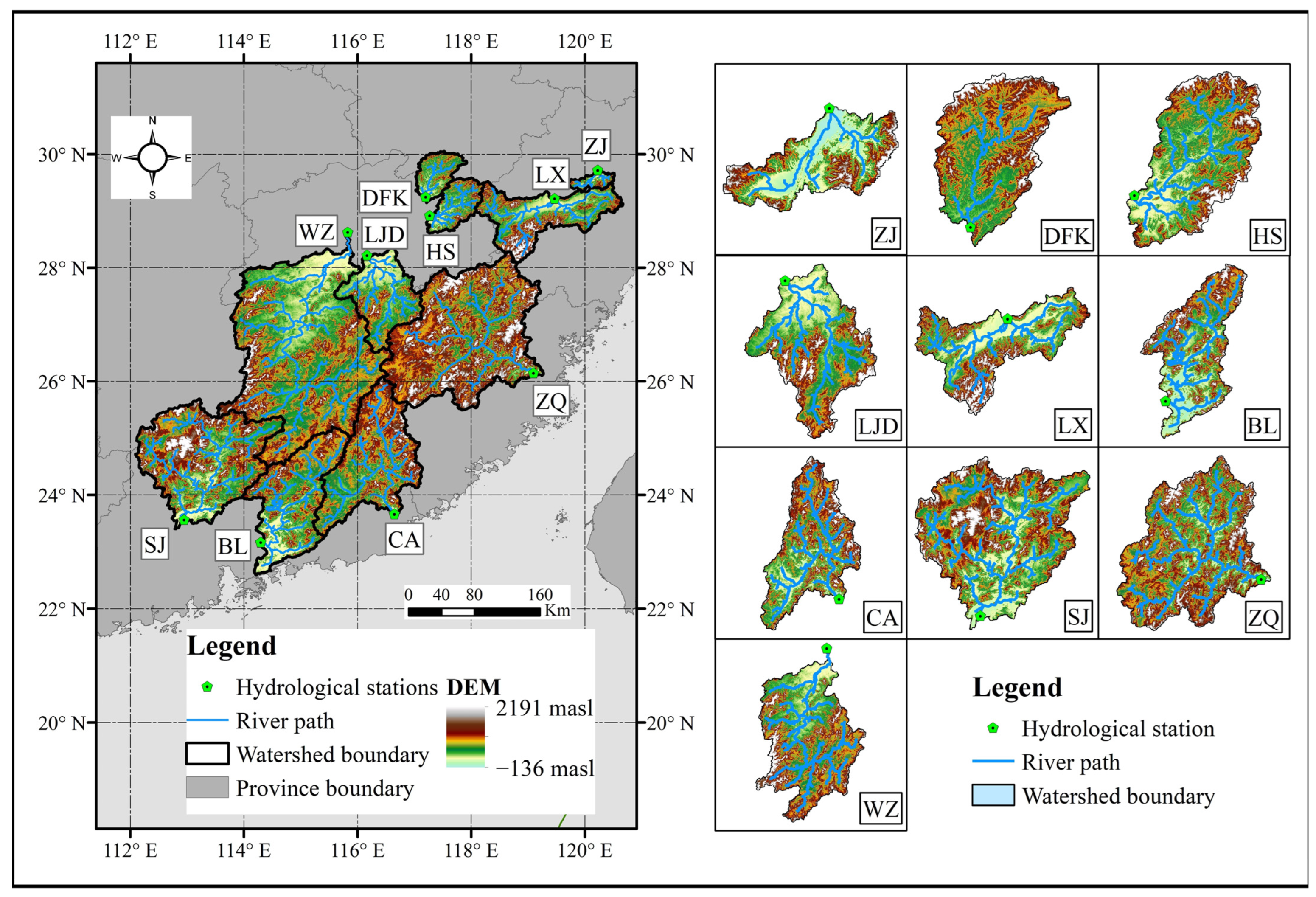
2. Study Area
3. Data and Methods
3.1. Data Description
3.2. LMs Selection
3.3. Hydrological Indices
3.4. Analysis Methods
- (1)
- The origin series and are: ; . The and series are the landscape series and hydrological indices, respectively; n is the series number, which corresponds to the year.
- (2)
- The clip correlation series for and were established. For the lag time of years, the and series are and , respectively. The value of ranges from 0 to 4, and it represents lag times of 0–4 years.
- (3)
- The correlation coefficient () between and was calculated, and the result was the lag correlation between and with a lag time of years. The highest value of with a significance of 0.05 was regarded as the lag time between and .
4. Results
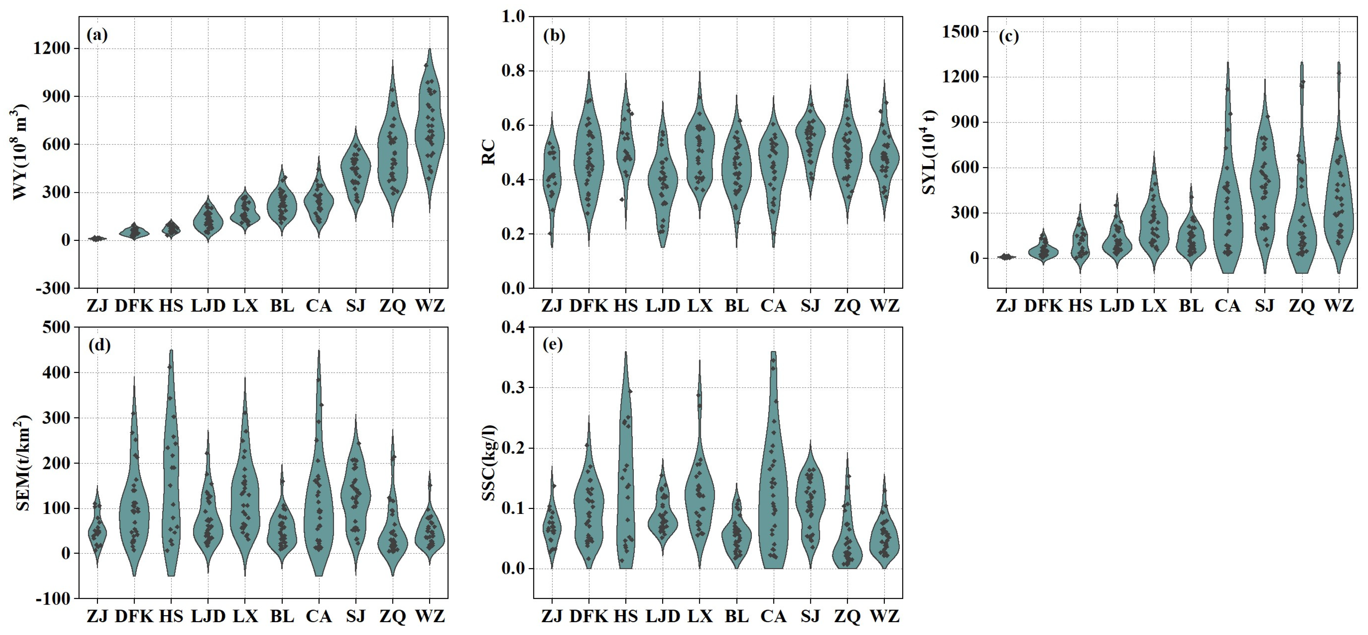
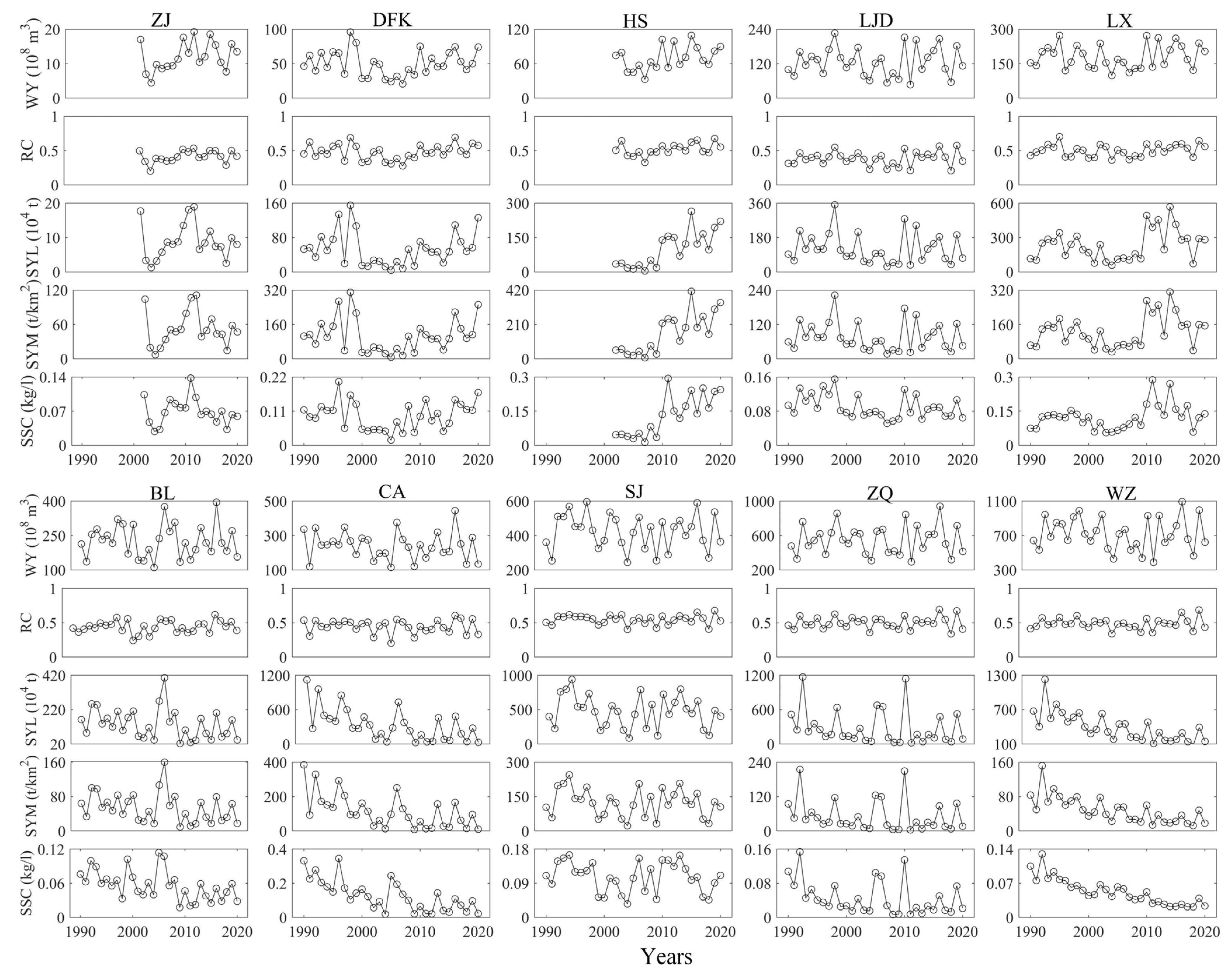
4.1. Variations in SY, RC, SYL, SEM, and SSC
4.2. Temporal Variations in LPs in the Chosen Watersheds
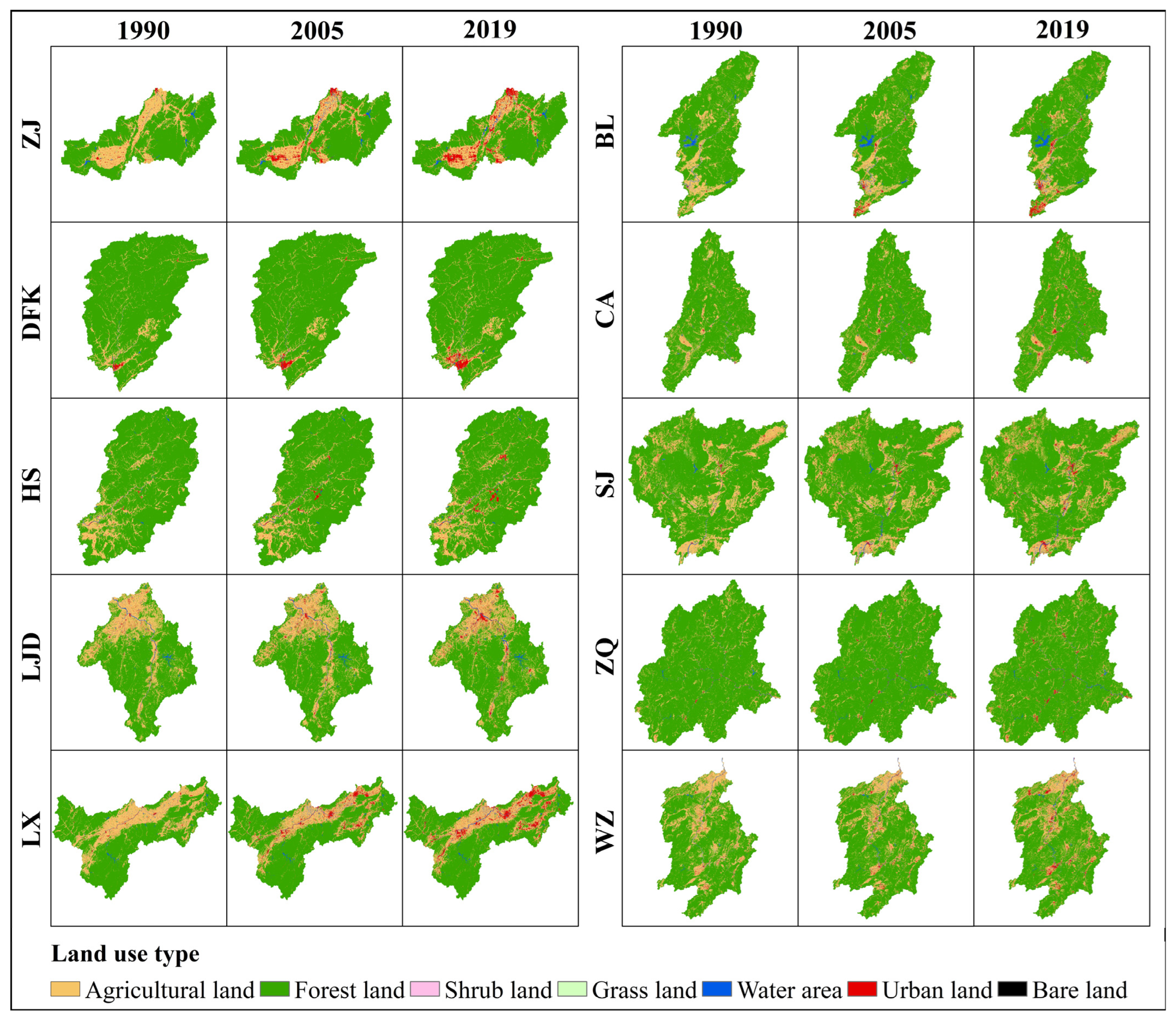
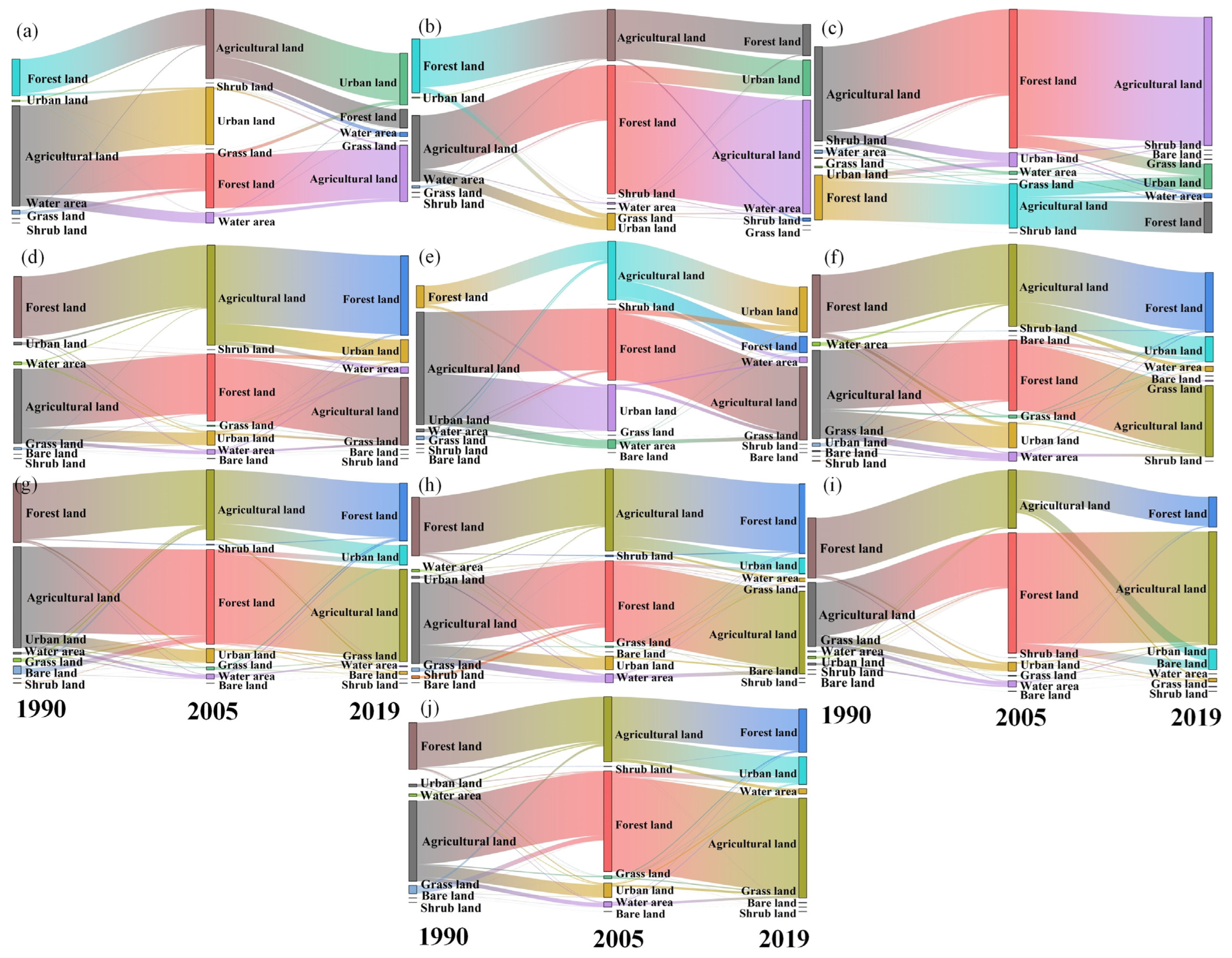
4.2.1. Land Use Changes from 1990 to 2019
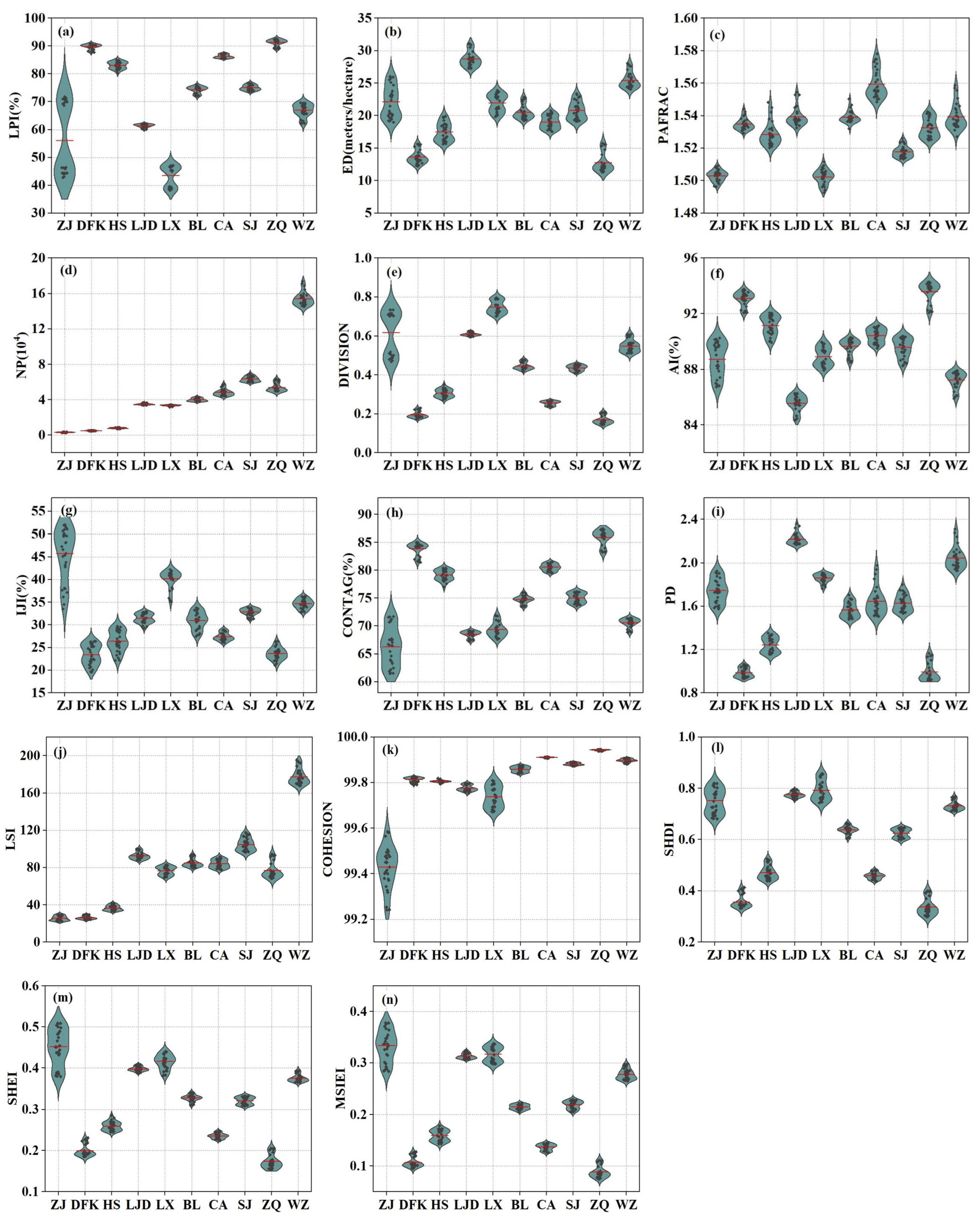
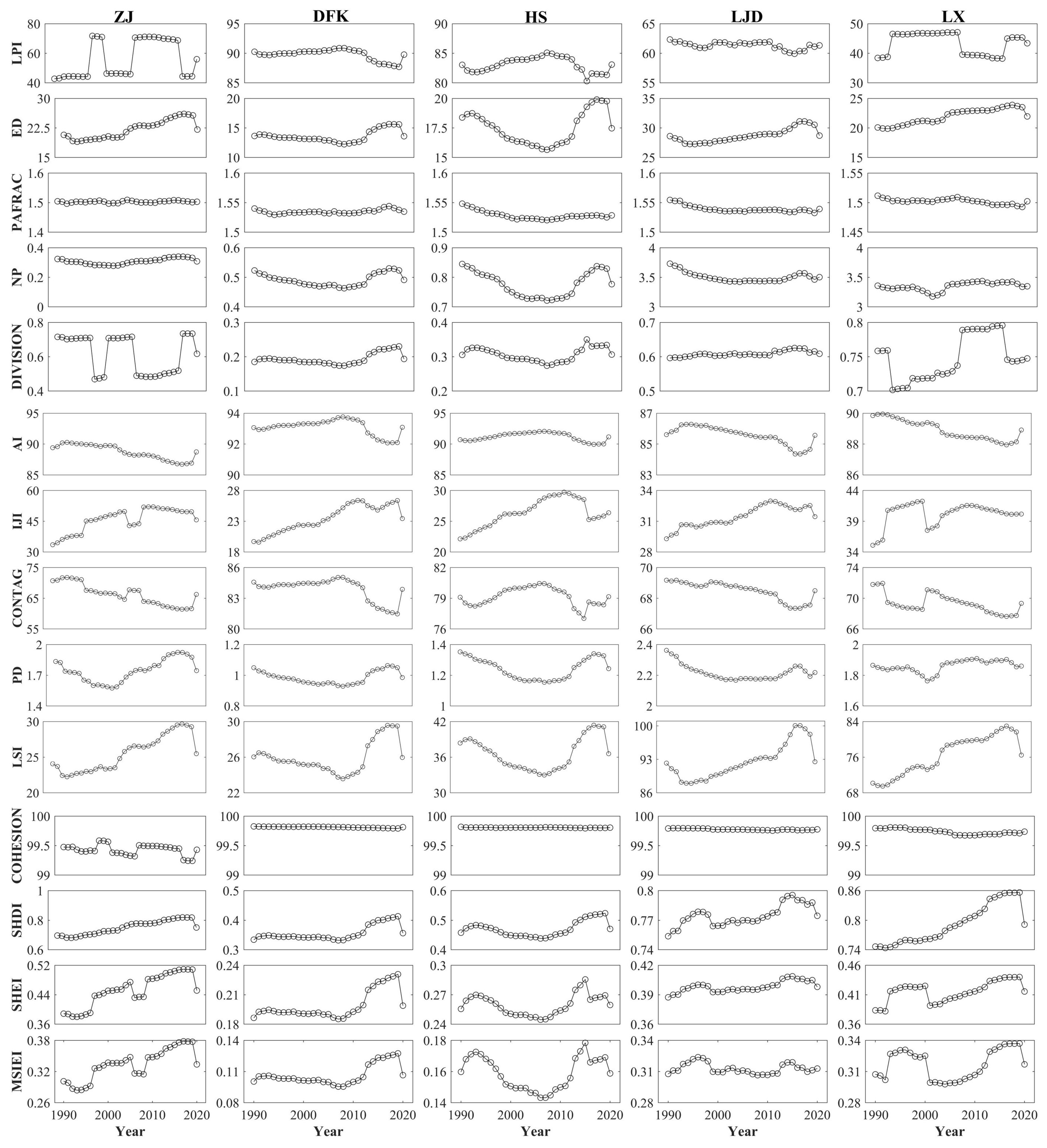
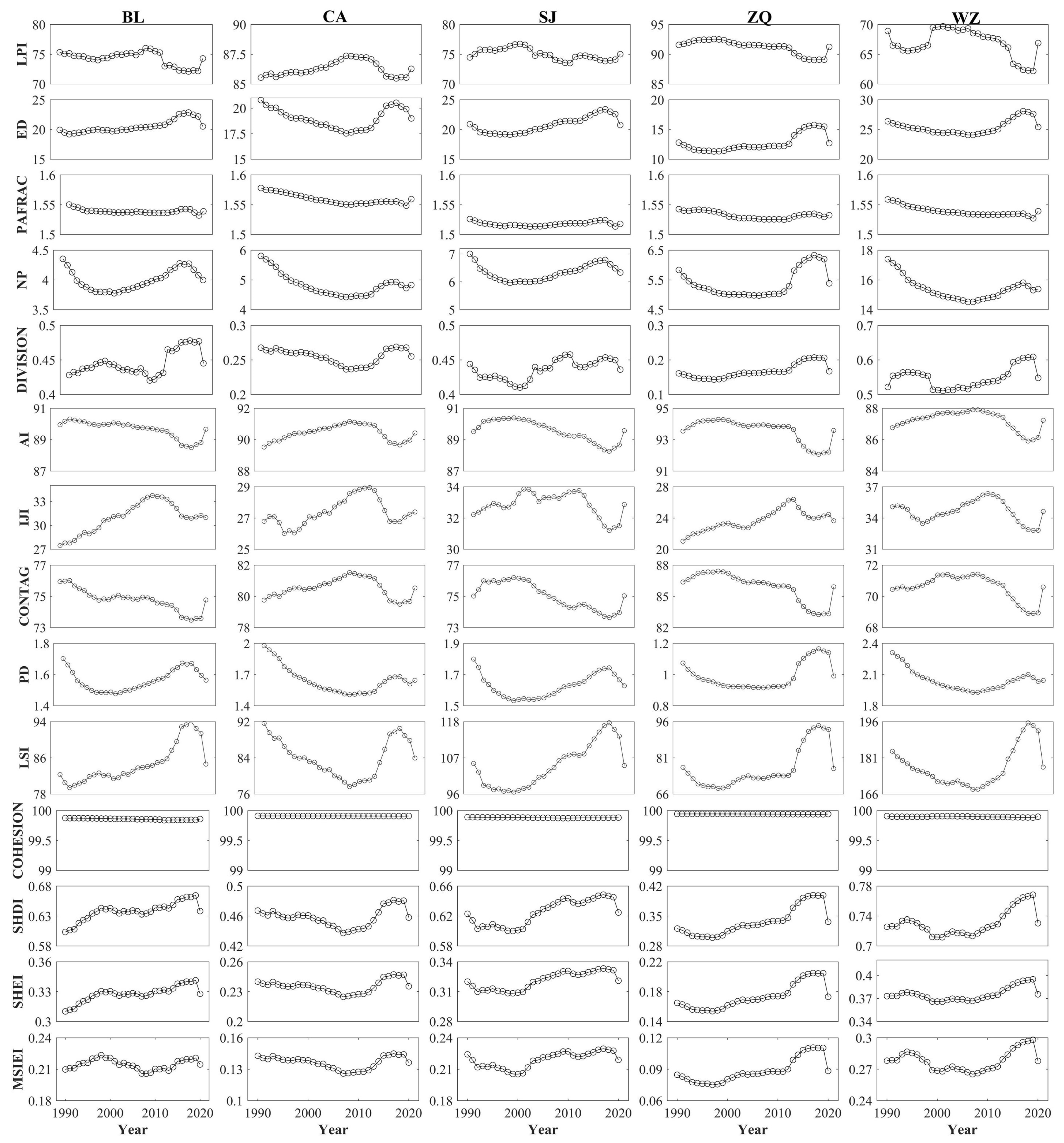
4.2.2. LM Changes from 1990 to 2019
4.3. Relationships between Hydrological Indices and LPs
5. Discussion
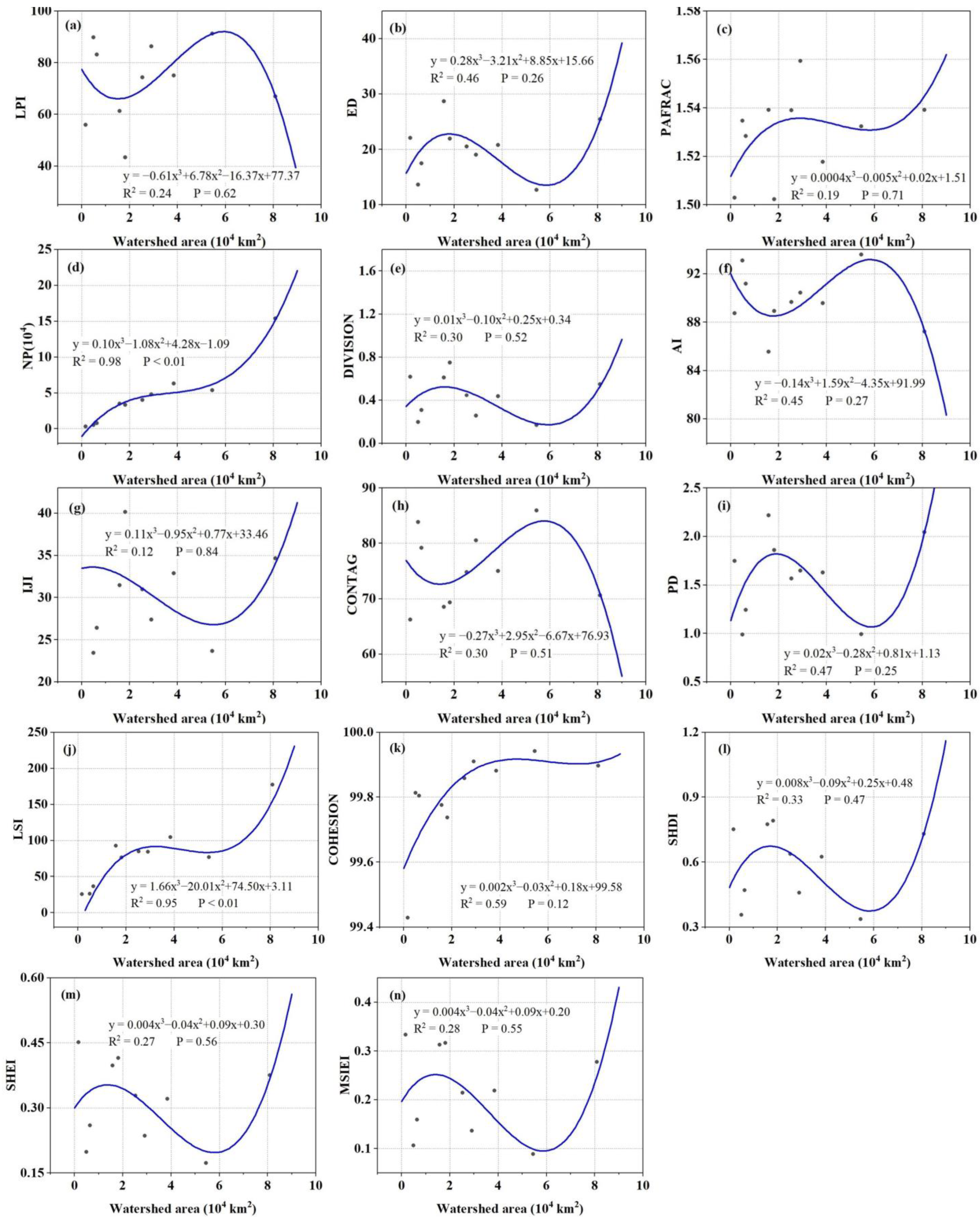
5.1. Correlations between LMs and Watershed Size
5.2. Effects of Various LMs on Hydrological Processes
5.3. Recommendations for LM Selection in Future Relevant Studies
5.4. Implications, Limitations, and Prospects
6. Conclusions
- (1)
- From 1990 to 2019, the change trends of WY and RC were not significant for any watersheds, and SEM and SSC decreased in all watersheds except for ZJ, HS, and LX. The main land use conversions were forest land–agricultural land, agricultural land–urban land, and agricultural land–forest land, and urban land expanded drastically in all watersheds. In addition, most LMs changed significantly (p < 0.05) for most watersheds, which demonstrates that LPs characteristics changed significantly.
- (2)
- For most watersheds (≥7), WY was negatively correlated with LPI, AI, CONTAG, and COHESION and positively correlated with ED, PAFRAC, DIVISION, LSI, SHDI, SHEI, and MSIEI; RC was negatively correlated with LPI, CONTAG, and COHESION and positively correlated with PAFRAC, DIVISION, SHDI, SHEI, and MSIEI; SEM was negatively correlated with LPI and IJI; SEM and SSC were positively correlated with PAFRAC, NP, PD, COHESION, and MSIEI. In addition, the effects of several LMs (IJI, SHDI, and SHEI) on WY, RC, and SEM had scale effects.
- (3)
- In the subtropical monsoon climate zone, runoff increases when a watershed is dominated by a small patch of landscape. In addition, landscape fragmentation and diversity also increase runoff. Proper landscape fragmentation and physical connectivity would benefit soil erosion and river and reservoir siltation prevention.
Author Contributions
Funding
Data Availability Statement
Conflicts of Interest
Glossary
| Abbreviation | Full name | Abbreviation | Full name |
| LP(s) | Landscape pattern(s) | LMs | Landscape metrics |
| WY | Water yields | RC | Runoff coefficient |
| SEM | Soil erosion modulus | SSC | Suspended sediment concentration |
| SYL | Sediment yields load | p | Significance level |
| NDCA | Number of disjunct core areas | PD | Patch density |
| LSI | Landscape shape index | SHDI | Shannon’s diversity index |
| DIVISION | Landscape division index | LPI | Largest patch index |
| COHESION | Patch cohesion index | MSIEI | Modified Simpson’s evenness index |
| AI | Aggregation index | ED | Edge density |
| PLAND | Percentage of landscape | SWAT | Soil and Water Assessment Tool |
| InVEST | Integrated Valuation of Ecosystem Services and Trade-offs | WaTEM/SEDEM | Water and Tillage Erosion Model and Sediment Delivery Model |
| RUSLE | Revised Universal Soil Loss Equation | IUH | Instantaneous Unit Hydrograph |
| HRUs | Hydrological response units | ZJ | Zhuji |
| DFK | Dufengkeng | HS | Hushan |
| LJD | Lijiadu | LX | Lanxi |
| BL | Boluo | CA | Chaoan |
| SJ | Shijiao | ZQ | Zhuqi |
| WZ | Waizhou | masl | Meters above the sea level |
| DA | Drainage area | AE | Average elevation |
| PRE | Precipitation | PAFRAC | Perimeter area fractal dimension |
| NP | Number of patches | IJI | Interspersion and Juxtaposition index |
| CONTAG | Contiguity index | SHEI | Shannon’s evenness index |
| R | Correlation coefficient |
Appendix A

| Categories | Metrics | Definition | Relevant Literature |
|---|---|---|---|
| Edge area | LPI | The ratio of the largest patch to the total landscape area. Unit (%) | [25,31,35,38,50,51] |
| ED | The length of the edges per unit area. Unit (Meters/hectare) | [25,38,50,51] | |
| Shape | PAFRAC | An index of patch shape complexity across a wide range of spatial scales. | [25,27,31,35,39,51] |
| Aggregation | NP | Extent of subdivision or fragmentation of the landscape pattern. | [31,35,38] |
| DIVISION | Reflects the degree of fragmentation of the landscape. Unit (Proportion) | [17,35,36] | |
| AI | Connectivity between patches of landscape types. Unit (%) | [25,31,38,50] | |
| IJI | The observed interspersion over the maximum possible interspersion for the given number of patch types. Unit (%) | [27,31,39,51] | |
| CONTAG | An index measuring the extent to which patch types are aggregated or clumped. Unit (%) | [25,31,33,35,38,50,51] | |
| PD | The number of patches within 1 km2. Unit (Number per 100 hectares) | [25,31,35,38,50,51] | |
| LSI | This index reflects the complexity of the boundaries of all patches within the region. | [31,35,50,51] | |
| COHESION | Measures the physical connectedness of the corresponding patch type. | [25,27,35,38,39,50,51] | |
| Diversity | SHDI | The number of different patch types and the proportional area distribution among patch types. | [25,33,35,38,50,51] |
| SHEI | The proportional abundance of each patch type. | [25,27,33,38,39] | |
| MSIEI | MSIEI equals minus the logarithm of the sum, across all patch types, of the proportional abundance of each patch type squared, which is then divided by the logarithm of the number of patch types. | [25,33] |


References
- Rasool, R.; Fayaz, A.; ul Shafiq, M.; Singh, H.; Ahmed, P. Land use land cover change in Kashmir Himalaya: Linking remote sensing with an indicator based DPSIR approach. Ecol. Indic. 2021, 125, 107447. [Google Scholar] [CrossRef]
- Terêncio, D.; Varandas, S.; Fonseca, A.; Cortes, R.; Fernandes, L.; Pacheco, F.; Monteiro, S.; Martinho, J.; Cabral, J.; Santos, J. Integrating ecosystem services into sustainable landscape management: A collaborative approach. Sci. Total Environ. 2021, 794, 148538. [Google Scholar] [CrossRef] [PubMed]
- Nafi′Shehab, Z.; Jamil, N.R.; Aris, A.Z.; Shafie, N.S. Spatial variation impact of landscape patterns and land use on water quality across an urbanized watershed in Bentong, Malaysia. Ecol. Indic. 2021, 122, 107254. [Google Scholar] [CrossRef]
- Devátý, J.; Dostál, T.; Hösl, R.; Krása, J.; Strauss, P. Effects of historical land use and land pattern changes on soil erosion–Case studies from Lower Austria and Central Bohemia. Land Use Policy 2019, 82, 674–685. [Google Scholar] [CrossRef]
- Sahin, V.; Hall, M.J. The effects of afforestation and deforestation on water yields. J. Hydrol. 1996, 178, 293–309. [Google Scholar] [CrossRef]
- Costa, M.H.; Botta, A.; Cardille, J.A. Effects of large-scale changes in land cover on the discharge of the Tocantins River, Southeastern Amazonia. J. Hydrol. 2003, 283, 206–217. [Google Scholar] [CrossRef]
- Kalantari, Z.; Lyon, S.W.; Folkeson, L.; French, H.K.; Stolte, J.; Jansson, P.E.; Sassner, M. Quantifying the hydrological impact of simulated changes in land use on peak discharge in a small catchment. Sci. Total Environ. 2014, 466–467, 741–754. [Google Scholar] [CrossRef]
- Wang, Z.P.; Tian, J.C.; Feng, K.P. Response of runoff towards land use changes in the Yellow River Basin in Ningxia, China. PLoS ONE 2022, 17, e0265931. [Google Scholar] [CrossRef]
- Wei, C.; Dong, X.; Yu, D.; Liu, J.; Reta, G.; Zhao, W.; Kuriqi, A.; Su, B. An alternative to the Grain for Green Program for soil and water conservation in the upper Huaihe River basin, China. J. Hydrol. Reg. Stud. 2022, 43, 101180. [Google Scholar] [CrossRef]
- Molinero-Parejo, R.; Aguilera-Benavente, F.; Gómez-Delgado, M.; Shurupov, N. Combining a land parcel cellular automata (LP-CA) model with participatory approaches in the simulation of disruptive future scenarios of urban land use change. Comput. Environ. Urban Syst. 2023, 99, 101895. [Google Scholar] [CrossRef]
- Liang, X.; Liu, X.; Li, X.; Chen, Y.; Tian, H.; Yao, Y. Delineating multi-scenario urban growth boundaries with a CA-based FLUS model and morphological method. Landsc. Urban Plan. 2018, 177, 47–63. [Google Scholar] [CrossRef]
- Xu, G.; Cheng, Y.; Zhao, C.; Mao, J.; Li, Z.; Jia, L.; Zhang, Y.; Wang, B. Effects of driving factors at multi-spatial scales on seasonal runoff and sediment changes. Catena 2023, 222, 106867. [Google Scholar] [CrossRef]
- Smetanova, A.; Follain, S.; David, M.; Ciampalini, R.; Raclot, D.; Crabit, A.; Le Bissonnais, Y. Landscaping compromises for land degradation neutrality: The case of soil erosion in a Mediterranean agricultural landscape. J. Environ. Manag. 2019, 235, 282–292. [Google Scholar] [CrossRef] [PubMed]
- Lacher, I.L.; Ahmadisharaf, E.; Fergus, C.; Akre, T.; Mcshea, W.J.; Benham, B.L.; Kline, K.S. Scale-dependent impacts of urban and agricultural land use on nutrients, sediment, and runoff. Sci. Total Environ. 2019, 652, 611–622. [Google Scholar] [CrossRef] [PubMed]
- Gonzales-Inca, C.A.; Kalliola, R.; Kirkkala, T.; Lepisto, A. Multiscale Landscape Pattern Affecting on Stream Water Quality in Agricultural Watershed, SW Finland. Water Resour. Manag. 2015, 29, 1669–1682. [Google Scholar] [CrossRef]
- McGarigal, K. FRAGSTATS: Spatial Pattern Analysis Program for Quantifying Landscape Structure; US Department of Agriculture, Forest Service, Pacific Northwest Research Station: La Grande, OR, USA, 1995; Volume 351.
- Bin, L.L.; Xu, K.; Xu, X.Y.; Lian, J.J.; Ma, C. Development of a landscape indicator to evaluate the effect of landscape pattern on surface runoff in the Haihe River Basin. J. Hydrol. 2018, 566, 546–557. [Google Scholar] [CrossRef]
- Shi, P.; Qin, Y.-L.; Li, P.; Li, Z.-B.; Cui, L.-Z. Development of a landscape index to link landscape pattern to runoff and sediment. J. Mt. Sci. 2022, 19, 2905–2919. [Google Scholar] [CrossRef]
- Wang, X.; Liu, X.; Wang, L.; Yang, J.; Wan, X.; Liang, T. A holistic assessment of spatiotemporal variation, driving factors, and risks influencing river water quality in the northeastern Qinghai-Tibet Plateau. Sci. Total Environ. 2022, 851, 157942. [Google Scholar] [CrossRef]
- Stets, E.G.; Sprague, L.A.; Oelsner, G.P.; Johnson, H.M.; Murphy, J.C.; Ryberg, K.; Vecchia, A.V.; Zuellig, R.E.; Falcone, J.A.; Riskin, M.L. Landscape drivers of dynamic change in water quality of US rivers. Environ. Sci Technol. 2020, 54, 4336–4343. [Google Scholar] [CrossRef]
- Liu, Y.; Shen, Y.; Cheng, C.; Yuan, W.; Gao, H.; Guo, P. Analysis of the influence paths of land use and landscape pattern on organic matter decomposition in river ecosystems: Focusing on microbial groups. Sci. Total Environ. 2022, 817, 153381. [Google Scholar] [CrossRef]
- Kumar, G.; Baweja, P.; Gandhi, P.B. Impact of Anthropogenic Activities on Soil Patterns and Diversity. In Structure and Functions of Pedosphere; Springer: Berlin/Heidelberg, Germany, 2022; pp. 319–337. [Google Scholar]
- Sadeghi, S.H.; Moradi Dashtpagerdi, M.; Moradi Rekabdarkoolai, H.; Schoorl, J.M. Sensitivity analysis of relationships between hydrograph components and landscapes metrics extracted from digital elevation models with different spatial resolutions. Ecol. Indic. 2021, 121, 107025. [Google Scholar] [CrossRef]
- Zhao, X.; Huang, G. Exploring the impact of landscape changes on runoff under climate change and urban development: Implications for landscape ecological engineering in the Yangmei River Basin. Ecol. Eng. 2022, 184, 106794. [Google Scholar] [CrossRef]
- Zhang, S.; Fan, W.; Li, Y.; Yi, Y. The influence of changes in land use and landscape patterns on soil erosion in a watershed. Sci. Total Environ. 2017, 574, 34–45. [Google Scholar] [CrossRef] [PubMed]
- Brini, I.; Alexakis, D.D.; Kalaitzidis, C. Linking Soil Erosion Modeling to Landscape Patterns and Geomorphometry: An Application in Crete, Greece. Appl. Sci. 2021, 11, 5684. [Google Scholar] [CrossRef]
- Zhou, Z.X.; Li, J. The correlation analysis on the landscape pattern index and hydrological processes in the Yanhe watershed, China. J. Hydrol. 2015, 524, 417–426. [Google Scholar] [CrossRef]
- Li, J.; Zhou, Y.; Li, Q.; Yi, S.; Peng, L. Exploring the Effects of Land Use Changes on the Landscape Pattern and Soil Erosion of Western Hubei Province from 2000 to 2020. Int. J. Environ. Res. Pub. Health 2022, 19, 1571. [Google Scholar] [CrossRef]
- Aghsaei, H.; Dinan, N.M.; Moridi, A.; Asadolahi, Z.; Delavar, M.; Fohrer, N.; Wagner, P.D. Effects of dynamic land use/land cover change on water resources and sediment yield in the Anzali wetland catchment, Gilan, Iran. Sci. Total Environ. 2020, 712, 136449. [Google Scholar] [CrossRef]
- Yohannes, H.; Soromessa, T.; Argaw, M.; Dewan, A. Impact of landscape pattern changes on hydrological ecosystem services in the Beressa watershed of the Blue Nile Basin in Ethiopia. Sci. Total Environ. 2021, 793, 148559. [Google Scholar] [CrossRef]
- Chen, C.; Zhao, G.; Zhang, Y.; Bai, Y.; Tian, P.; Mu, X.; Tian, X. Linkages between soil erosion and long-term changes of landscape pattern in a small watershed on the Chinese Loess Plateau. Catena 2023, 220, 106659. [Google Scholar] [CrossRef]
- Wei, C.; Dong, X.; Ma, Y.; Gou, J.; Li, L.; Bo, H.; Yu, D.; Su, B. Applicability comparison of various precipitation products of long-term hydrological simulations and their impact on parameter sensitivity. J. Hydrol. 2023, 618, 129187. [Google Scholar] [CrossRef]
- Ouyang, W.; Skidmore, A.K.; Hao, F.; Wang, T. Soil erosion dynamics response to landscape pattern. Sci. Total Environ. 2010, 408, 1358–1366. [Google Scholar] [CrossRef] [PubMed]
- Xiao, R.; Cao, W.; Liu, Y.; Lu, B. The impacts of landscape patterns spatio-temporal changes on land surface temperature from a multi-scale perspective: A case study of the Yangtze River Delta. Sci. Total Environ. 2022, 821, 153381. [Google Scholar] [CrossRef] [PubMed]
- Yang, Y.Y.; Li, Z.B.; Li, P.; Ren, Z.P.; Gao, H.D.; Wang, T.; Xu, G.C.; Yu, K.X.; Shi, P.; Tang, S.S. Variations in runoff and sediment in watersheds in loess regions with different geomorphologies and their response to landscape patterns. Environ. Earth Sci. 2017, 76, 517. [Google Scholar] [CrossRef]
- Zhang, Y.; Bi, Z.L.; Zhang, X.; Yu, Y. Influence of Landscape Pattern Changes on Runoff and Sediment in the Dali River Watershed on the Loess Plateau of China. Land 2019, 8, 180. [Google Scholar] [CrossRef]
- Gao, F.; He, B.; Xue, S.S.; Li, Y.Z. Impact of landscape pattern change on runoff processes in catchment area of the Ulungur River Basin. Water Supply 2020, 20, 1046–1058. [Google Scholar] [CrossRef]
- Wei, C.; Zhang, Z.; Wang, Z.; Cao, L.; Wei, Y.; Zhang, X.; Zhao, R.; Xiao, L.; Wu, Q. Response of Variation of Water and Sediment to Landscape Pattern in the Dapoling Watershed. Sustainability 2022, 14, 678. [Google Scholar] [CrossRef]
- Li, J.; Zhou, Z.X. Coupled analysis on landscape pattern and hydrological processes in Yanhe watershed of China. Sci. Total Environ. 2015, 505, 927–938. [Google Scholar] [CrossRef]
- Chiang, L.-C.; Wang, Y.-C.; Chen, Y.-K.; Liao, C.-J. Quantification of land use/land cover impacts on stream water quality across Taiwan. J. Clean Prod. 2021, 318, 128443. [Google Scholar] [CrossRef]
- Ke, Q.; Zhang, K. Patterns of runoff and erosion on bare slopes in different climate zones. Catena 2021, 198, 105069. [Google Scholar] [CrossRef]
- Zhu, X.; Li, T.; Tian, Z.; Qu, L.; Liang, Y. Building pedotransfer functions for estimating soil erodibility in southeastern China. Ecol. Indic. 2022, 145, 109720. [Google Scholar] [CrossRef]
- Wei, C.; Dong, X.; Yu, D.; Zhang, T.; Zhao, W.; Ma, Y.; Su, B. Spatio-temporal variations of rainfall erosivity, correlation of climatic indices and influence on human activities in the Huaihe River Basin, China. Catena 2022, 217, 106486. [Google Scholar] [CrossRef]
- Yang, J.; Huang, X. The 30 m annual land cover dataset and its dynamics in China from 1990 to 2019. Earth Syst. Sci. Data 2021, 13, 3907–3925. [Google Scholar] [CrossRef]
- Liang, L.; Yu, L.; Wang, Z. Identifying the dominant impact factors and their contributions to heatwave events over mainland China. Sci. Total Environ. 2022, 848, 157527. [Google Scholar] [CrossRef] [PubMed]
- Wang, L.; Han, X.; Zhang, Y.; Zhang, Q.; Wan, X.; Liang, T.; Song, H.; Bolan, N.; Shaheen, S.M.; White, J.R. Impacts of land uses on spatio-temporal variations of seasonal water quality in a regulated river basin, Huai River, China. Sci. Total Environ. 2023, 857, 159584. [Google Scholar] [CrossRef]
- Lisha, Q.; Qiuan, Z.; Chaofan, Z.; Jiang, Z. Monthly Precipitation Data Set with 1 km Resolution in China from 1960 to 2020[DS/OL]. Science Data Bank: Beijing, China, 2022; Available online: https://cstr.cn/31253.11.sciencedb.01607.CSTR:31253.11.sciencedb.01607 (accessed on 25 December 2022).
- Xu, S.; Li, S.-L.; Zhong, J.; Li, C. Spatial scale effects of the variable relationships between landscape pattern and water quality: Example from an agricultural karst river basin, Southwestern China. Agric. Ecosyst. Environ. 2020, 300, 106999. [Google Scholar] [CrossRef]
- Han, Y.; Wang, J.-l.; Li, P. Influences of landscape pattern evolution on regional crop water requirements in regions of large-scale agricultural operations. J. Clean Prod. 2021, 327, 129499. [Google Scholar] [CrossRef]
- Jinying, X.; Yang, B.; Hailin, Y.; Xiaowei, W.; Zhifei, M.; Hongwei, Z. Water quality assessment and the influence of landscape metrics at multiple scales in Poyang Lake basin. Ecol. Indic. 2022, 141, 109096. [Google Scholar] [CrossRef]
- Shi, Z.H.; Ai, L.; Li, X.; Huang, X.D.; Wu, G.L.; Liao, W. Partial least-squares regression for linking land-cover patterns to soil erosion and sediment yield in watersheds. J. Hydrol. 2013, 498, 165–176. [Google Scholar] [CrossRef]
- Machado, R.E.; Cardoso, T.O.; Mortene, M.H. Determination of runoff coefficient (C) in catchments based on analysis of precipitation and flow events. Int. Soil Water Conserv. Res. 2022, 10, 208–216. [Google Scholar] [CrossRef]
- Romano, G.; Abdelwahab, O.M.; Gentile, F. Modeling land use changes and their impact on sediment load in a Mediterranean watershed. Catena 2018, 163, 342–353. [Google Scholar] [CrossRef]
- Wu, L.; Yao, W.W.; Ma, X.Y. Using the comprehensive governance degree to calibrate a piecewise sediment delivery ratio algorithm for dynamic sediment predictions: A case study in an ecological restoration watershed of northwest China. J. Hydrol. 2018, 564, 888–899. [Google Scholar] [CrossRef]
- Wang, J.; Shi, B.; Zhao, E.; Yuan, Q.; Chen, X. The long-term spatial and temporal variations of sediment loads and their causes of the Yellow River Basin. Catena 2022, 209, 105850. [Google Scholar] [CrossRef]
- Weisberg, S. Applied Linear Regression; John Wiley & Sons: Hoboken, NJ, USA, 2005; Volume 528. [Google Scholar]
- Parhizkar, M.; Shabanpour, M.; Lucas-Borja, M.E.; Zema, D.A. Variability of rill detachment capacity with sediment size, water depth and soil slope in forest soils: A flume experiment. J. Hydrol. 2021, 601, 126625. [Google Scholar] [CrossRef]
- Dall′Agnol, R.; Sahoo, P.K.; Salomao, G.N.; de Araujo, A.D.M.; da Silva, M.S.; Powell, M.A.; Ferreira, J.; Ramos, S.J.; Martins, G.C.; da Costa, M.F.; et al. Soil-sediment linkage and trace element contamination in forested/deforested areas of the Itacaiunas River Watershed, Brazil: To what extent land-use change plays a role? Sci. Total Environ. 2022, 828, 154327. [Google Scholar] [CrossRef] [PubMed]
- Tiku, M. Tables of the power of the F-test. J. Am. Stat. Assoc. 1967, 62, 525–539. [Google Scholar] [CrossRef]
- Meals, D.W.; Dressing, S.A.; Davenport, T.E. Lag Time in Water Quality Response to Best Management Practices: A Review. J. Environ. Qual. 2010, 39, 85–96. [Google Scholar] [CrossRef]
- Li, Y.; Li, Y.R.; Fang, B.; Wang, Q.Y.; Chen, Z.F. Impacts of ecological programs on land use and ecosystem services since the 1980s: A case-study of a typical catchment on the Loess Plateau, China. Land Degrad. Dev. 2022, 33, 3271–3282. [Google Scholar] [CrossRef]
- Fenicia, F.; McDonnell, J.J. Modeling streamflow variability at the regional scale: (1) perceptual model development through signature analysis. J. Hydrol. 2022, 605, 127287. [Google Scholar] [CrossRef]
- Schilling, K.E.; Wolter, C.F. A GIS-based groundwater travel time model to evaluate stream nitrate concentration reductions from land use change. Environ. Geol. 2007, 53, 433–443. [Google Scholar] [CrossRef]
- Barlow, K.M.; Weeks, A.; Christy, B. Modelling the response in streamflow to increased forestry plantations. In Proceedings of the 20th International Congress on Modelling and Simulation (MODSIM), Adelaide, Australia, 1–6 December 2013; pp. 538–544. [Google Scholar]
- He, D.; Chen, Z.; Zhou, J.; Yang, T.; Lu, L. The Heterogeneous Impact of High-Speed Railway on Urban Expansion in China. Remote Sens. 2021, 13, 4914. [Google Scholar] [CrossRef]
- Mostafa, E.; Li, X.; Sadek, M.; Dossou, J.F. Monitoring and Forecasting of Urban Expansion Using Machine Learning-Based Techniques and Remotely Sensed Data: A Case Study of Gharbia Governorate, Egypt. Remote Sens. 2021, 13, 4498. [Google Scholar] [CrossRef]
- Sarkodie, S.A.; Owusu, P.A. Global land-use intensity and anthropogenic emissions exhibit symbiotic and explosive behavior. Iscience 2022, 25, 104741. [Google Scholar] [CrossRef] [PubMed]
- Shi, P.; Zhang, Y.; Ren, Z.; Yu, Y.; Li, P.; Gong, J. Land-use changes and check dams reducing runoff and sediment yield on the Loess Plateau of China. Sci. Total Environ. 2019, 664, 984–994. [Google Scholar] [CrossRef] [PubMed]
- Dong, H.; Song, Y.; Chen, L.; Liu, H.; Fu, X.; Xie, M. Soil erosion and human activities over the last 60 years revealed by magnetism, particle size and minerals of check dams sediments on the Chinese Loess Plateau. Environ. Earth Sci. 2022, 81, 162. [Google Scholar] [CrossRef]
- Fan, J.; Xu, Y.; Ge, H.; Yang, W. Vegetation growth variation in relation to topography in Horqin Sandy Land. Ecol. Indic. 2020, 113, 106215. [Google Scholar] [CrossRef]
- Zhang, Z.D.; Chen, S.J.; Wan, L.W.; Cao, J.; Zhang, Q.; Yang, C.X. The effects of landscape pattern evolution on runoff and sediment based on SWAT model. Environ. Earth Sci. 2021, 80, 2. [Google Scholar] [CrossRef]
- Deng, Y.; Wu, S.; Ke, J.; Zhu, A. Effects of meteorological factors and groundwater depths on plant sap flow velocities in karst critical zone. Sci. Total Environ. 2021, 781, 146764. [Google Scholar] [CrossRef]
- Yang, M.; Li, X.Z.; Hu, Y.M.; He, X.Y. Assessing effects of landscape pattern on sediment yield using sediment delivery distributed model and a landscape indicator. Ecol. Indic. 2012, 22, 38–52. [Google Scholar] [CrossRef]
- Ma, B.; Wu, C.; Ding, F.; Zhou, Z. Predicting basin water quality using source-sink landscape distribution metrics in the Danjiangkou Reservoir of China. Ecol. Indic. 2021, 127, 107697. [Google Scholar] [CrossRef]
- Ouyang, W.; Wu, Y.; Hao, Z.; Zhang, Q.; Bu, Q.; Gao, X. Combined impacts of land use and soil property changes on soil erosion in a mollisol area under long-term agricultural development. Sci. Total Environ. 2018, 613, 798–809. [Google Scholar] [CrossRef]
- de Carvalho, D.F.; Macedo, P.M.S.; Pinto, M.F.; de Almeida, W.S.; Schultz, N. Soil loss and runoff obtained with customized precipitation patterns simulated by InfiAsper. Int. Soil Water Conserv. Res. 2022, 10, 407–413. [Google Scholar] [CrossRef]
- Pijl, A.; Reuter, L.E.; Quarella, E.; Vogel, T.A.; Tarolli, P. GIS-based soil erosion modelling under various steep-slope vineyard practices. Catena 2020, 193, 104604. [Google Scholar] [CrossRef]
- Zhu, X.; Liang, Y.; Tian, Z.; Wang, X. Analysis of scale-specific factors controlling soil erodibility in southeastern China using multivariate empirical mode decomposition. Catena 2021, 199, 105131. [Google Scholar] [CrossRef]
- Wallace, M.; Mickovski, S.B.; Griffin, I. An innovative framework for selecting sustainable options to reduce the risk of soil erosion and environmental pollution incidents on road construction sites. In Proceedings of the XVII ECSMGE-2019: Geotechnical Engineering Foundation of the Future, Reykjavik, Iceland, 1–6 September 2019; The Icelandic Geotechnical Society: Reykjavik, Iceland, 2019. [Google Scholar]
- Zhang, Y.F.; Wang, N.; Tang, C.J.; Zhang, S.Q.; Song, Y.J.; Liao, K.T.; Nie, X.F. A New Indicator to Better Represent the Impact of Landscape Pattern Change on Basin Soil Erosion and Sediment Yield in the Upper Reach of Ganjiang, China. Land 2021, 10, 990. [Google Scholar] [CrossRef]
- Rufí-Salís, M.; Petit-Boix, A.; Villalba, G.; Sanjuan-Delmás, D.; Parada, F.; Ercilla-Montserrat, M.; Arcas-Pilz, V.; Munoz-Liesa, J.; Rieradevall, J.; Gabarrell, X. Recirculating water and nutrients in urban agriculture: An opportunity towards environmental sustainability and water use efficiency? J. Clean Prod. 2020, 261, 121213. [Google Scholar] [CrossRef]
- Trang, T.T.; Bush, S.R.; van Leeuwen, J. Enhancing institutional capacity in a centralized state: The case of industrial water use efficiency in Vietnam. J. Ind. Ecol. 2022, 27, 210–222. [Google Scholar] [CrossRef]


| Stations | DA (km2) | AE (m) | PRE (mm) | WY (108 m3) | RC | SYL (104 t) | SEM (t/km2) | SSC (mg/L) |
|---|---|---|---|---|---|---|---|---|
| ZJ | 1700 | 232 | 1686 | 12.17 | 0.41 | 8.90 | 52.38 | 0.07 |
| DFK | 5000 | 243 | 2054 | 50.44 | 0.48 | 52.97 | 105.94 | 0.09 |
| HS | 6400 | 255 | 2162 | 71.01 | 0.52 | 104.16 | 162.75 | 0.13 |
| LJD | 15,800 | 222 | 2003 | 124.99 | 0.39 | 120.76 | 76.43 | 0.09 |
| LX | 18,200 | 352 | 1942 | 180.89 | 0.50 | 232.69 | 127.85 | 0.12 |
| BL | 25,300 | 288 | 2006 | 222.21 | 0.44 | 131.96 | 52.16 | 0.05 |
| CA | 29,100 | 397 | 1825 | 235.32 | 0.45 | 321.79 | 110.58 | 0.12 |
| SJ | 38,400 | 384 | 1994 | 416.69 | 0.55 | 463.70 | 120.75 | 0.11 |
| ZQ | 54,500 | 533 | 1982 | 544.55 | 0.50 | 278.93 | 51.18 | 0.04 |
| WZ | 80,900 | 300 | 1812 | 713.52 | 0.49 | 382.66 | 47.30 | 0.05 |
| Indices | ZJ | DFK | HS | LJD | LX | BL | CA | SJ | ZQ | WZ |
|---|---|---|---|---|---|---|---|---|---|---|
| WY | 0.25 | −0.003 | 1.53 | 0.16 | 0.64 | −0.12 | −1.22 | −1.00 | 0.75 | −1.13 |
| RC | 0.0048 | 0.0012 | 0.0064 | 0.0008 | 0.0016 | 0.0013 | −0.0009 | −0.0001 | 0.0008 | 0.0004 |
| SYL | 0.04 | −0.02 | 10.90 ** | −1.19 | 4.43 | −3.04 | −19.01 ** | −4.72 | −7.63 | −19.76 ** |
| SEM | 0.23 | −0.04 | 17.03 ** | −0.75 | 2.43 | −1.20 | −6.53 ** | −1.23 | −1.40 | −2.44 ** |
| SSC | −0.0005 | 0.0002 | 0.0128 ** | −0.0011 * | 0.0019 | −0.0015 ** | −0.0073 ** | −0.0008 | −0.0016 * | −0.0026 ** |
| Metrics | ZJ | DFK | HS | LJD | LX | BL | CA | SJ | ZQ | WZ |
|---|---|---|---|---|---|---|---|---|---|---|
| LPI | 0.62 * | −0.06 ** | −0.01 | −0.04 * | −0.09 | −0.08 ** | 0.02 | −0.07 ** | −0.11 ** | −0.11 * |
| ED | 0.26 ** | 0.05 * | 0.03 | 0.12 ** | 0.15 ** | 0.11 ** | −0.01 | 0.14 ** | 0.13 ** | 0.06 * |
| PAFRAC | 0.0001 | 0.0002 ** | −0.0005 ** | −0.0005 ** | −0.0004 ** | −0.0002 ** | −0.0009 ** | 0.00005 | −0.0004 ** | −0.0008 ** |
| NP | 0.0013 ** | 0.0004 | −0.0006 | −0.0045 ** | 0.0045 ** | 0.0072 | −0.0264 ** | 0.0108 | 0.0263 ** | −0.0436 ** |
| DIVISION | −0.0043 | 0.0010 ** | 0.0002 | 0.0007 ** | 0.0021 ** | 0.0013 ** | −0.0003 | 0.0011 ** | 0.020 ** | 0.0014 * |
| AI | −0.129 ** | −0.025 * | −0.015 | −0.058 ** | −0.074 ** | −0.054 ** | 0.007 | −0.068 ** | −0.065 ** | −0.029 * |
| IJI | 0.55 ** | 0.24 ** | 0.18 ** | 0.11 ** | 0.08 * | 0.16 ** | 0.05 * | −0.03 | 0.12 ** | −0.02 |
| CONTAG | −0.376 ** | −0.082 ** | −0.14 | −0.063 ** | −0.097 ** | −0.073 ** | −0.001 | −0.087 ** | −0.137 ** | −0.049 ** |
| PD | 0.008 ** | 0.001 | −0.001 | −0.003 ** | 0.002 ** | 0.003 | −0.009 ** | 0.003 | 0.005 ** | −0.006 ** |
| LSI | 0.27 ** | 0.09 * | 0.06 | 0.36 ** | 0.50 ** | 0.44 ** | −0.06 | 0.67 ** | 0.76 ** | 0.39 * |
| COHESION | −0.0034 | −0.0011 ** | −0.0003 ** | −0.0013 ** | −0.0045 ** | −0.0013 ** | −0.0001 ** | −0.0005 ** | −0.0003 ** | −0.0005 ** |
| SHDI | 0.005 ** | 0.002 ** | 0.001 * | 0.001 ** | 0.004 ** | 0.002 ** | 0.001 | 0.002 ** | 0.003 ** | 0.001 ** |
| SHEI | 0.005 ** | 0.001 ** | 0.001 | 0.001 ** | 0.001 ** | 0.001 ** | 0.001 | 0.001 ** | 0.002 ** | 0.001 ** |
| MSIEI | 0.0031 ** | 0.0006 ** | 0 | −0.0001 | 0.0005 | 0 | −0.0001 | 0.0006 ** | 0.0011 ** | 0.0003 |
| Hydrological Indices | LMs | ZJ | DFK | HS | LJD | LX | BL | CA | SJ | ZQ | WZ |
|---|---|---|---|---|---|---|---|---|---|---|---|
| WY | LPI | 0.57 1 | −0.28 0 | −0.46 0 | −0.29 1 | −0.46 3 | −0.22 1 | −0.21 0 | 0.28 1 | −0.08 0 | −0.40 4 |
| ED | 0.48 1 | 0.27 0 | 0.39 0 | −0.03 1 | 0.14 4 | 0.13 0 | 0.25 2 | −0.13 1 | 0.10 0 | 0.29 2 | |
| PAFRAC | −0.12 2 | 0.12 0 | 0.50 0 | 0.16 3 | −0.33 1 | 0.21 2 | 0.24 2 | 0.34 4 | 0.19 2 | 0.26 2 | |
| NP | 0.53 1 | 0.33 1 | 0.33 0 | 0.16 2 | 0.37 4 | 0.20 3 | 0.27 2 | 0.30 4 | 0.19 2 | 0.35 2 | |
| DIVISION | −0.56 1 | 0.28 0 | 0.46 0 | 0.16 1 | 0.36 3 | 0.22 1 | 0.21 0 | −0.28 1 | 0.08 0 | 0.39 4 | |
| AI | −0.48 1 | −0.27 0 | −0.39 0 | 0.03 1 | −0.14 4 | −0.13 0 | −0.25 2 | 0.13 1 | −0.10 0 | −0.29 2 | |
| IJI | 0.47 1 | −0.11 0 | 0.60 4 | 0.08 4 | 0.11 0 | −0.17 2 | −0.26 0 | −0.26 3 | 0.14 4 | −0.35 0 | |
| CONTAG | −0.47 1 | −0.23 0 | −0.53 1 | −0.12 0 | −0.24 0 | −0.12 0 | −0.22 2 | 0.18 1 | −0.09 0 | −0.31 4 | |
| PD | 0.53 1 | 0.33 1 | 0.33 0 | 0.16 2 | 0.37 4 | 0.20 3 | 0.27 2 | 0.30 4 | 0.19 2 | 0.35 2 | |
| LSI | 0.48 1 | 0.27 0 | 0.39 0 | −0.03 1 | 0.14 4 | 0.13 0 | 0.25 2 | −0.13 1 | 0.10 0 | 0.29 2 | |
| COHESION | 0.59 3 | −0.16 4 | −0.51 0 | 0.16 2 | −0.21 4 | −0.08 4 | −0.09 4 | 0.30 2 | −0.11 3 | −0.33 4 | |
| SHDI | 0.50 1 | 0.20 0 | 0.41 0 | 0.26 1 | 0.17 4 | −0.16 3 | 0.18 0 | −0.21 1 | 0.08 0 | 0.32 4 | |
| SHEI | 0.46 1 | 0.20 0 | 0.54 1 | 0.26 1 | 0.27 0 | −0.16 3 | 0.18 0 | −0.21 1 | 0.08 0 | 0.32 4 | |
| MSIEI | 0.34 0 | 0.25 0 | 0.48 0 | 0.32 1 | 0.34 0 | −0.13 3 | 0.21 0 | −0.23 1 | 0.08 1 | 0.30 2 | |
| RC | LPI | 0.58 1 | −0.44 0 | −0.55 0 | −0.28 0 | −0.52 3 | −0.34 1 | −0.27 2 | 0.19 1 | −0.18 0 | −0.41 1 |
| ED | 0.45 1 | 0.43 0 | 0.50 0 | 0.11 3 | 0.18 4 | 0.30 0 | 0.30 2 | 0.13 4 | 0.19 0 | 0.39 2 | |
| PAFRAC | −0.17 3 | 0.28 0 | 0.53 1 | −0.12 0 | −0.33 0 | 0.14 2 | 0.21 2 | 0.37 4 | 0.14 2 | 0.16 2 | |
| NP | 0.49 1 | 0.44 1 | 0.48 2 | 0.17 2 | 0.33 4 | 0.27 3 | 0.25 2 | 0.31 4 | 0.25 2 | 0.31 2 | |
| DIVISION | −0.57 1 | 0.44 0 | 0.55 0 | 0.22 0 | 0.41 3 | 0.34 1 | 0.27 2 | −0.19 1 | 0.18 0 | 0.41 1 | |
| AI | −0.45 1 | −0.43 0 | −0.50 0 | −0.11 3 | −0.18 4 | −0.30 0 | −0.30 2 | −0.13 4 | −0.19 0 | −0.39 2 | |
| IJI | 0.48 1 | 0.18 4 | 0.63 4 | 0.13 4 | −0.19 3 | −0.09 2 | −0.28 0 | −0.25 3 | 0.18 4 | −0.42 0 | |
| CONTAG | −0.46 1 | −0.40 0 | −0.57 1 | −0.19 0 | −0.22 0 | −0.28 0 | −0.29 2 | 0.09 1 | −0.18 0 | −0.40 3 | |
| PD | 0.49 1 | 0.44 1 | 0.48 2 | 0.18 2 | 0.33 4 | 0.27 3 | 0.25 2 | 0.31 4 | 0.25 2 | 0.31 2 | |
| LSI | 0.45 1 | 0.43 0 | 0.50 0 | 0.11 3 | 0.18 4 | 0.30 0 | 0.30 2 | 0.13 4 | 0.19 0 | 0.39 2 | |
| COHESION | 0.59 3 | −0.34 4 | −0.54 0 | 0.12 1 | −0.24 4 | −0.19 1 | −0.17 4 | 0.222 | −0.18 3 | −0.37 4 | |
| SHDI | 0.47 1 | 0.38 0 | 0.51 0 | 0.28 0 | 0.24 4 | 0.25 0 | 0.28 2 | −0.11 1 | 0.18 0 | 0.40 3 | |
| SHEI | 0.45 1 | 0.38 0 | 0.58 1 | 0.28 0 | 0.27 0 | 0.24 0 | 0.28 2 | −0.11 1 | 0.18 0 | 0.40 3 | |
| MSIEI | 0.33 1 | 0.42 0 | 0.56 1 | 0.28 0 | 0.35 0 | 0.18 0 | 0.27 2 | −0.13 1 | 0.18 1 | 0.39 2 |
| Hydrological Indices | LMs | ZJ | DFK | HS | LJD | LX | BL | CA | SJ | ZQ | WZ |
|---|---|---|---|---|---|---|---|---|---|---|---|
| SEM | LPI | 0.62 1 | −0.30 2 | −0.72 0 | −0.18 1 | −0.63 3 | 0.16 0 | −0.44 3 | −0.35 3 | 0.13 0 | −0.21 4 |
| ED | 0.24 1 | 0.27 3 | 0.69 0 | −0.15 0 | 0.34 4 | −0.25 0 | 0.42 2 | −0.17 0 | −0.12 0 | 0.35 4 | |
| PAFRAC | −0.33 0 | −0.10 2 | 0.76 0 | 0.29 2 | −0.46 0 | 0.30 2 | 0.63 0 | 0.34 3 | 0.17 2 | 0.82 2 | |
| NP | 0.30 1 | 0.41 3 | 0.66 0 | 0.27 2 | 0.59 4 | −0.16 0 | 0.58 0 | 0.32 3 | 0.13 2 | 0.71 2 | |
| DIVISION | −0.63 1 | 0.30 2 | 0.72 0 | −0.13 2 | 0.59 3 | −0.17 0 | 0.44 3 | 0.34 3 | −0.13 0 | 0.20 4 | |
| AI | −0.24 1 | −0.27 3 | −0.69 0 | 0.15 0 | −0.34 4 | 0.25 0 | −0.42 2 | 0.17 0 | 0.12 0 | −0.35 4 | |
| IJI | −0.75 4 | −0.16 3 | 0.76 4 | −0.16 2 | 0.33 0 | −0.36 2 | −0.45 2 | 0.12 1 | −0.29 2 | −0.30 4 | |
| CONTAG | 0.64 4 | −0.23 2 | −0.76 0 | 0.07 2 | −0.44 0 | 0.30 2 | −0.38 3 | 0.18 0 | 0.14 0 | 0.21 0 | |
| PD | 0.30 1 | 0.41 3 | 0.66 0 | 0.27 2 | 0.59 4 | −0.16 0 | 0.58 0 | 0.32 3 | 0.13 2 | 0.71 2 | |
| LSI | 0.24 1 | 0.27 3 | 0.69 0 | −0.15 0 | 0.34 4 | −0.25 0 | 0.42 2 | −0.17 0 | −0.12 0 | 0.35 4 | |
| COHESION | 0.53 1 | −0.09 1 | −0.73 0 | 0.28 2 | −0.48 4 | 0.33 2 | 0.47 0 | 0.21 2 | 0.14 0 | 0.35 2 | |
| SHDI | 0.27 1 | 0.20 2 | 0.72 0 | 0.14 1 | 0.36 0 | −0.31 2 | 0.31 3 | −0.18 0 | −0.14 0 | −0.24 0 | |
| SHEI | −0.69 4 | 0.20 2 | 0.77 0 | 0.14 1 | 0.47 0 | −0.31 2 | 0.31 3 | −0.18 0 | −0.14 0 | −0.24 0 | |
| MSIEI | −0.74 4 | 0.26 2 | 0.75 0 | 0.35 1 | 0.42 0 | 0.15 4 | 0.41 3 | 0.25 3 | −0.25 0 | 0.25 4 | |
| SSC | LPI | 0.52 1 | −0.34 2 | −0.65 0 | 0.18 2 | −0.58 2 | 0.30 0 | −0.50 3 | −0.45 3 | 0.21 0 | 0.23 0 |
| ED | −0.37 4 | 0.34 3 | 0.68 0 | −0.35 0 | 0.34 4 | −0.44 0 | 0.48 4 | −0.15 0 | −0.17 0 | 0.26 4 | |
| PAFRAC | −0.49 0 | 0.16 0 | 0.78 0 | 0.54 2 | −0.41 0 | 0.35 2 | 0.70 0 | 0.27 3 | 0.26 0 | 0.89 2 | |
| NP | −0.41 4 | 0.45 3 | 0.66 0 | 0.51 4 | 0.61 3 | −0.22 0 | 0.62 0 | 0.26 3 | 0.12 2 | 0.74 4 | |
| DIVISION | −0.53 1 | 0.34 2 | 0.65 0 | −0.34 2 | 0.55 2 | −0.32 0 | 0.50 3 | 0.44 3 | −0.21 0 | −0.23 0 | |
| AI | 0.37 4 | −0.34 3 | −0.68 0 | 0.35 0 | −0.34 4 | 0.44 0 | −0.48 4 | 0.15 0 | 0.17 0 | −0.27 4 | |
| IJI | −0.71 4 | −0.09 3 | 0.73 4 | −0.36 2 | 0.39 0 | −0.49 2 | −0.51 2 | 0.19 1 | −0.38 2 | −0.36 4 | |
| CONTAG | 0.73 4 | −0.30 3 | −0.70 0 | 0.24 2 | −0.46 0 | 0.46 0 | −0.45 4 | −0.16 4 | 0.22 0 | 0.33 0 | |
| PD | −0.41 4 | 0.45 3 | 0.66 0 | 0.51 4 | 0.61 3 | −0.22 0 | 0.62 0 | 0.26 3 | 0.12 2 | 0.74 4 | |
| LSI | −0.37 4 | 0.34 3 | 0.68 0 | −0.35 0 | 0.34 4 | −0.44 0 | 0.48 4 | −0.15 0 | −0.17 0 | 0.26 4 | |
| COHESION | 0.53 0 | −0.20 1 | −0.66 0 | 0.46 0 | −0.47 4 | 0.49 0 | 0.59 0 | 0.15 0 | 0.26 0 | 0.49 2 | |
| SHDI | −0.36 4 | 0.28 3 | 0.72 0 | −0.20 4 | 0.37 0 | −0.44 0 | 0.38 4 | 0.19 4 | −0.23 0 | −0.37 0 | |
| SHEI | −0.75 4 | 0.28 3 | 0.70 0 | −0.20 4 | 0.47 0 | −0.44 0 | 0.38 4 | 0.19 4 | −0.23 0 | −0.37 0 | |
| MSIEI | −0.74 4 | 0.32 3 | 0.70 0 | 0.43 0 | 0.38 0 | 0.32 4 | 0.47 3 | 0.33 3 | −0.35 0 | −0.15 0 |
Disclaimer/Publisher’s Note: The statements, opinions and data contained in all publications are solely those of the individual author(s) and contributor(s) and not of MDPI and/or the editor(s). MDPI and/or the editor(s) disclaim responsibility for any injury to people or property resulting from any ideas, methods, instructions or products referred to in the content. |
© 2023 by the authors. Licensee MDPI, Basel, Switzerland. This article is an open access article distributed under the terms and conditions of the Creative Commons Attribution (CC BY) license (https://creativecommons.org/licenses/by/4.0/).
Share and Cite
Wei, C.; Dong, X.; Ma, Y.; Leng, M.; Zhao, W.; Zhang, C.; Yu, D.; Su, B. Relationships between Landscape Patterns and Hydrological Processes in the Subtropical Monsoon Climate Zone of Southeastern China. Remote Sens. 2023, 15, 2290. https://doi.org/10.3390/rs15092290
Wei C, Dong X, Ma Y, Leng M, Zhao W, Zhang C, Yu D, Su B. Relationships between Landscape Patterns and Hydrological Processes in the Subtropical Monsoon Climate Zone of Southeastern China. Remote Sensing. 2023; 15(9):2290. https://doi.org/10.3390/rs15092290
Chicago/Turabian StyleWei, Chong, Xiaohua Dong, Yaoming Ma, Menghui Leng, Wenyi Zhao, Chengyan Zhang, Dan Yu, and Bob Su. 2023. "Relationships between Landscape Patterns and Hydrological Processes in the Subtropical Monsoon Climate Zone of Southeastern China" Remote Sensing 15, no. 9: 2290. https://doi.org/10.3390/rs15092290