1. Introduction
The Tibetan Plateau, located in the interior of the Asian continent, is the highest plateau in the world. It has a total area of about 2.5 × 10
6 km
2 and an average elevation >4000 m (about 600 hPa) with a variety of landforms. The climate of the Tibetan Plateau is controlled by cold high-pressure systems (anticyclones) in winter, whereas in summer, the main controls are thermal depressions (cyclones) in the lower atmosphere and the South Asian high at upper levels [
1]. The thermodynamic and dynamic effects of the atmosphere over and around the Tibetan Plateau affect the local atmospheric circulation and also propagate outward via Rossby waves [
2]. This region, therefore, has a significant impact on the climate of Asia and the wider world [
3,
4].
There has been much research over a long period of time on the dynamic fields of the atmosphere over the Tibetan Plateau. The huge Tibetan Plateau has a significant blocking effect [
5]. Mid-latitude westerly winds encounter the plateau while moving eastward. Part of the airflow is forced to lift over the plateau, whereas the other part is deflected into two branches to the north and south, both of which continue to move eastward along the edges of the plateau. The flows around the plateau have more significant effects and change with the season [
6]. The northern branch is generally stronger than the southern branch [
7].
The two airflows pass through different areas and lead to different types of weather. The northern branch generates an anticyclonic circulation north of the plateau, leading to cold advection on the northeast side [
8]. Variations in the intensity of the flow affect temperatures in its eastern and southern regions—for example, in Northeast China and the Jianghuai region (downstream along the Yangtze River) to the east of the Tibetan Plateau [
9,
10]. The northern branch also influences the intensity of precipitation on the southeastern side of the plateau in South China [
11]. By contrast, the southern branch bends cyclonically on the south side of the plateau, forming a semi-permanent low-pressure trough (the south trough), which splits the subtropical high in this region [
8] and forms southwesterly warm advection to the southeast of the plateau. This branch affects the outbreak and persistence of the South Asian summer monsoon, in addition to the spatial and temporal distribution of precipitation in Eastern China [
12,
13,
14,
15,
16]. There has not been enough attention paid to how the dynamic effects of the atmosphere over and around the Tibetan Plateau influence the strength of advection in the northern and southern branches, further affecting the climate on the eastern side.
The cold northern branch and the warm southern branch converge on the eastern side of the plateau, resulting in different climatic phenomena at different times of the year. In spring and summer, the northern and southern branches flowing around the plateau converge in the downstream areas of the Yangtze River (in Jianghuai region), affecting the local distribution of temperature and rainfall [
7,
17,
18,
19]. In winter, guided by the anticyclone circulation formed by thermal action over the Tibetan Plateau, the northern airflow merges with cold air from the north and moves southward. Where it is blocked by the terrain of the Yunnan–Guizhou Plateau, and it meets the southwesterly warm air brought by the southern branch to form a quasi-stationary front (the Kunming quasi-stationary front) between Kunming and Guiyang. The weather varies on the two sides of the front. It is relatively wet with rain or sometimes snow on the cold northern side (e.g., in Guizhou, Sichuan and Chongqing). The warm southern side in Yunnan and other regions is controlled by a warm air mass, with sunshine and little rainfall. If the cold air flow is stronger, then the quasi-stationary front moves southward, leading to more rain in Yunnan [
20,
21]. There have been few studies of the mechanisms by which the dynamic effects of the atmosphere over and around the Tibetan Plateau influence the position of the intersection between warm and cold advection.
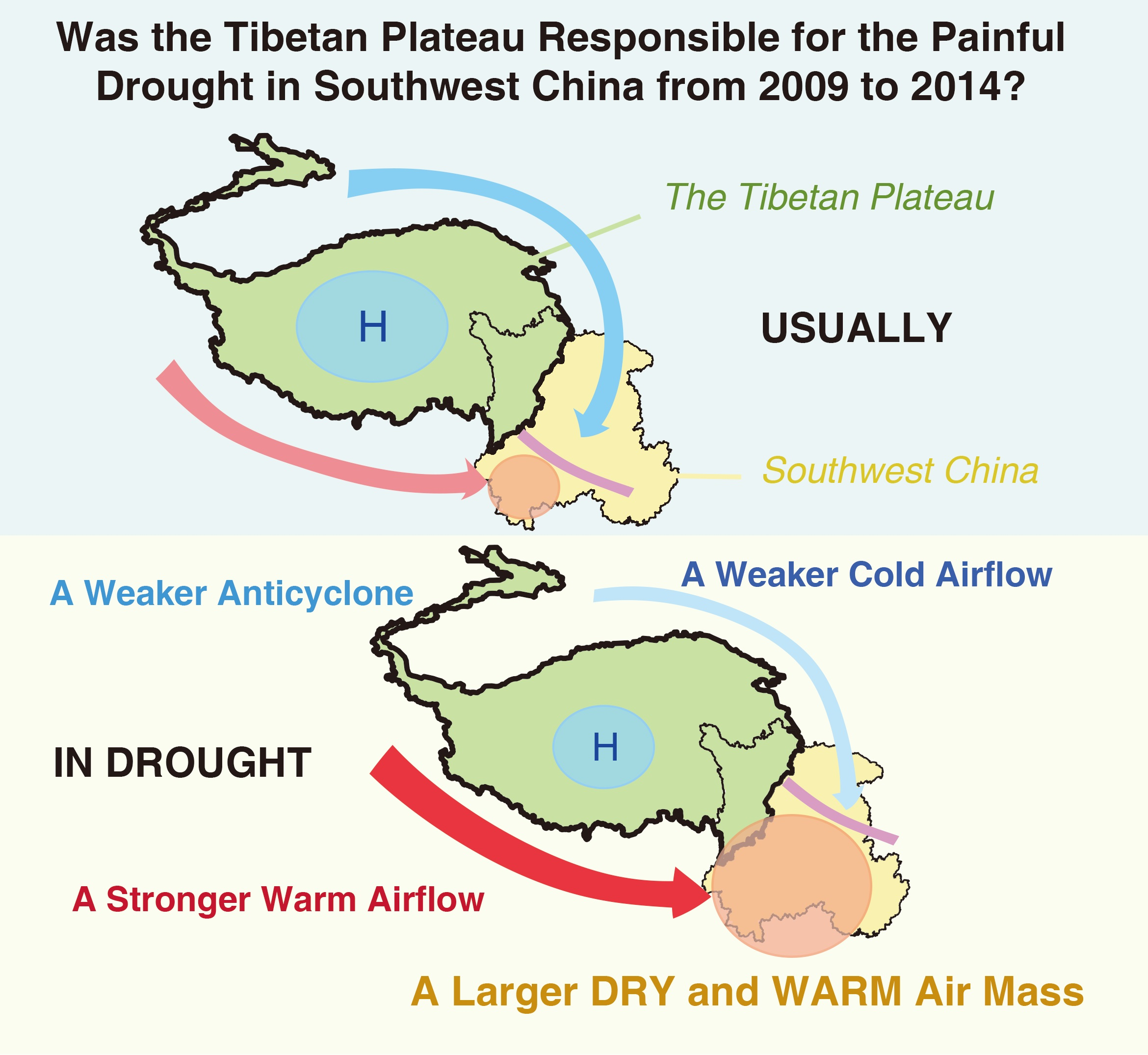
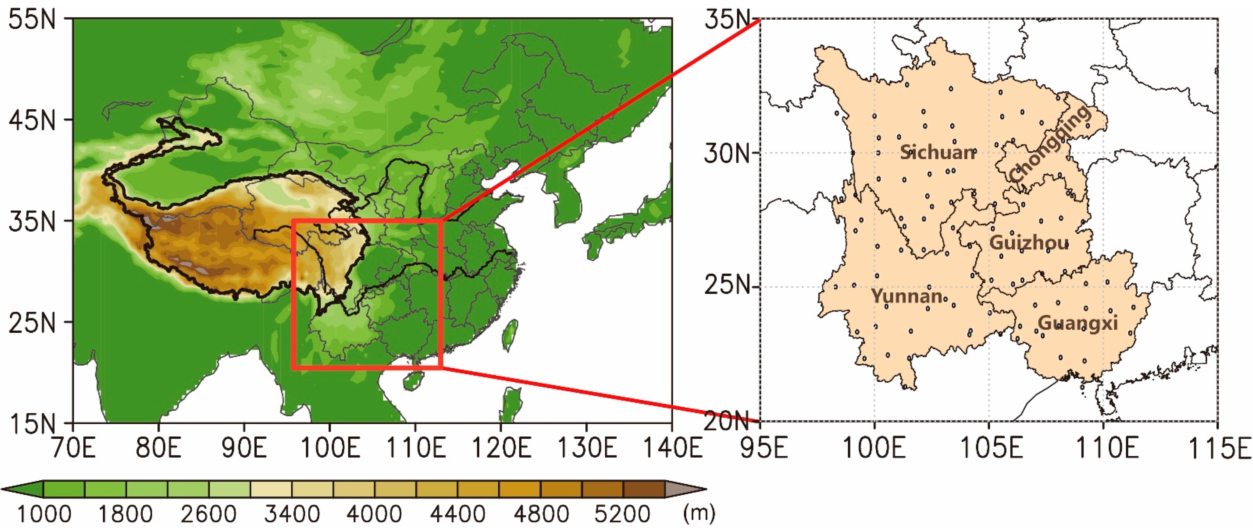
Winter rainfall in Southwest China is primarily generated by the quasi-stationary front in this region and should therefore be affected by the westerly flow around the Tibetan Plateau. Southwest China suffered severe droughts in winter and spring for five consecutive years from 2009 to 2014 (compared to the average of the same seasons in 1960–2019) (
Figure 1). There has been a variety of research about drought using different metrics or indexes. For example, Aksoy et al. [
22] raised a methodology related to the standardized precipitation index (SPI) to develop critical drought intensity–duration–frequency (IDF) curves; Huang et al. [
23] used SPI and Standardized Runoff Index (SRI), as well as Copula functions, to study the temporal and spatial evolution of meteorological drought and hydrological drought in the Jinghe River Basin by driving SWAT model. Here, we adopted the Percentage of Precipitation Anomaly, complying with the Chinese official document GBT20481-2017 [
24], to characterize this drought event in Southwest China by its spatial and temporal distributions, as well as its severity. In autumn 2009, precipitation was more than 50% lower than the average in central and eastern Yunnan, western Guizhou, northwestern Guangxi and the southern margin of Chongqing. Some areas in central Yunnan had a >80% reduction in precipitation, reaching the level of extreme drought (regions in the darkest red). The drought worsened during the winter of 2009. Almost the whole of Yunnan, southwest Guizhou and a major part of Sichuan experienced moderate-to-severe drought, and large areas of Yunnan and southwest Sichuan were affected by severe drought. This drought caused water shortages for 25 million people in the winter of 2009 and the following spring, resulting in 660 × 104 ha of crop failure in Yunnan, Guizhou, Guangxi and Sichuan provinces and >40 billion yuan of direct economic losses [
25,
26,
27]. In 2011, a severe drought in this region affected 39.52 million people, with 11.882 million people suffering shortages of freshwater and total economic losses of 21.8 billion yuan. The drought in Southwest China in 2013–2014 was rated as one of the top ten weather and climate events in China [
25,
26,
27].
Anomalous precipitation in Southwest China is closely related to the position of the confluence between warm and cold advection. However, it is unclear whether the circulation over the Tibetan Plateau during this period of extreme drought was different from the average field, so there would be unusual changes in the westerly flow around the Tibetan Plateau, leading to abnormal rainfall in Southwest China.
The work reported here is based on a statistical analysis of the dynamic fields over the Tibetan Plateau and precipitation in Southwest China from 1960 to 2019. It focuses on the continuous drought event in Southwest China from 2009 to 2014 and explores the mechanisms by which the dynamic fields over the Tibetan Plateau affected the precipitation anomaly in Southwest China. A regression model is proposed for the dynamic fields over the plateau and precipitation in Southwest China. The results of this study will contribute to the prediction of precipitation in Southwest China and encourage further research about how the flow around the Tibetan Plateau affects the climate on its eastern side.
2. Data and Methods
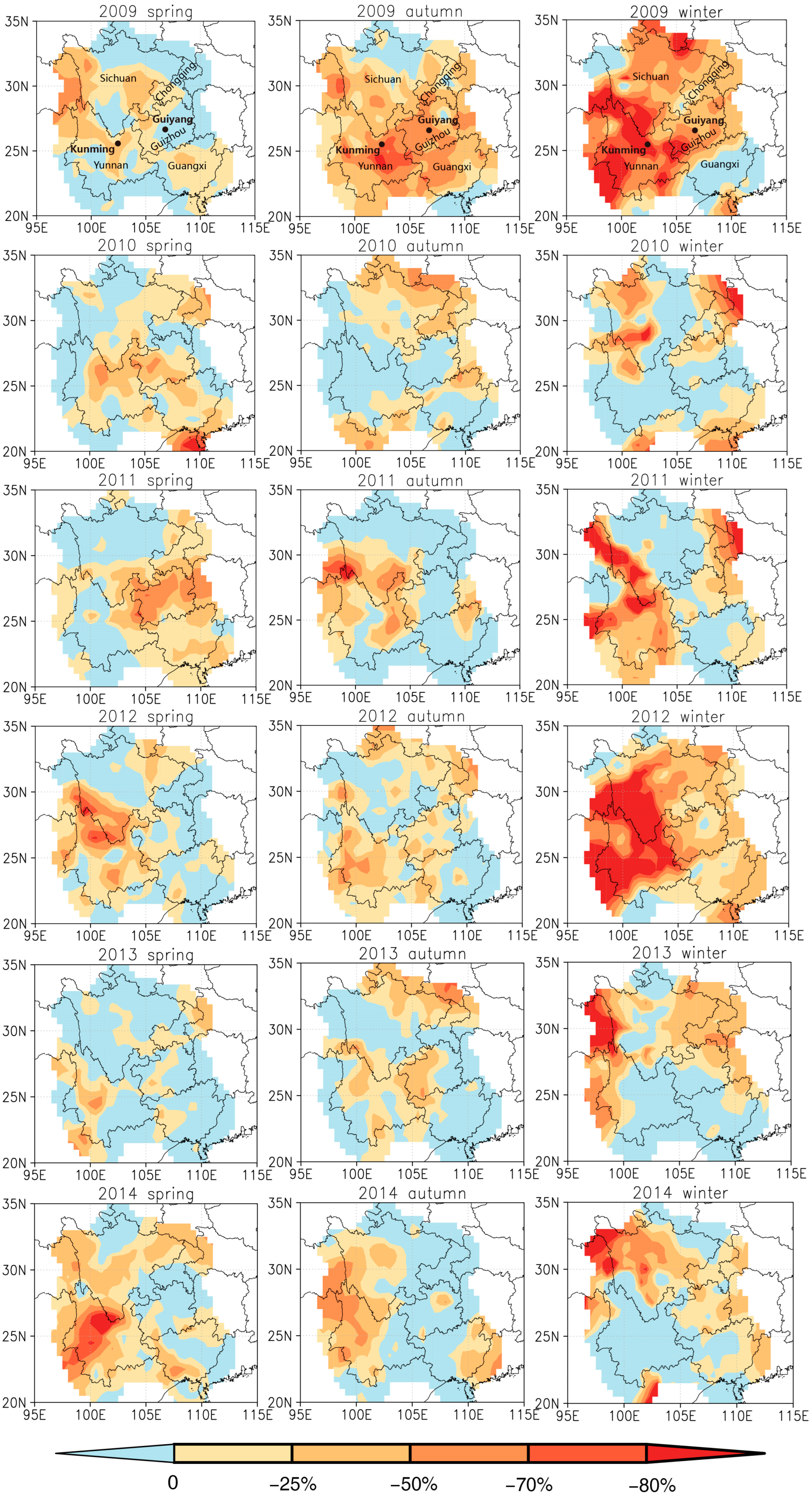
The data and methods used in the paper and the results are shown in
Figure 2. Two kinds of data were used in the paper. The first was the reanalysis data (including dynamic elements such as relative divergence, relative vorticity and horizontal and vertical wind velocity) from the Japanese 55-year Reanalysis (JRA-55), which was used to analyze the dynamical characteristics of the atmosphere over and around the Tibetan Plateau. The other was a precipitation observation from meteorological stations in Southwest China, which was used to introduce the drought event that happened in 2009–2014. In
Section 3 and
Section 4, to study the relation between the Tibetan Plateau and the severe drought in Southwest China, these two kinds of data were connected using statistical methods, such as empirical orthogonal function (EOF) and regression.
2.1. Data
It was found that the Japanese Reanalysis and the European Centre for Medium-Range Weather Forecasts (ECMWF) ReAnalysis (–ERA) datasets can better describe surface air temperatures and vertical wind velocity in China. In addition, the Japanese 55-year Reanalysis (JRA-55) is the most stable dataset over China [
28,
29]. Therefore, the dynamic field data of the Tibetan Plateau used in this paper was taken from the JRA-55 reanalysis data set, and the time range was 1960.1–2020.2. The latitude and longitude range of the Tibetan Plateau is 25°N–46°N, 75°E–105°E (see
Figure 3), the spatial resolution of which was 1.25° × 1.25°. The meteorological elements we used included relative divergence, relative vorticity, vertical velocity and wind speed. For the isobaric surface, 600 hPa, 500 hPa, 400 hPa, 300 hPa, 200 hPa and 100 hPa were selected. As the mean altitude of the Tibetan Plateau is over 3000 m (about 700 hPa), selections begin at 600 hPa to avoid any effects from the boundary layer.
In order to ensure the reliability of the data, the ERA-5 dataset with higher accuracy 0.25° × 0.25° was also analyzed with the same method and compared with the JRA-55 data, and it was found that the distribution of elements was similar. Therefore, the JRA-55 dataset was considered reliable.
The precipitation data of Southwest China used in this was from ‘Dataset of monthly climate data from Chinese surface stations’ (
http://101.200.76.197:93/data/cdcdetail/dataCode/SURF_CLI_CHN_MUL_MON.html, accessed on 1 February 2021). The data is quality controlled as the true rate of each meteorological element item data is generally more than 99%, and the accuracy rate of data is close to 100%. The observation data in the files of the monthly surface report from the national station from 1951 till now were repeatedly tested and controlled for quality, during which the incorrect records were corrected, and missing data were supplemented, which significantly improved the data quality. In addition, the quality controls and verifications for meteorological indices from 1951 till now were carried out during the production of the dataset, and the suspicious and incorrect values were generally checked and corrected manually. Finally, all meteorological indices were marked with quality control codes.
In this paper, Southwest China refers to Yunnan, Sichuan, Guangxi, Guizhou provinces and Chongqing Municipality (see
Figure 3). Only national stations established before 1960 with data records were counted, which yielded a total of 104 stations.
2.2. Methods
Empirical Orthogonal Function (EOF) is a method of analyzing the structural features of matrices and extracting the characteristic quantities of major data. It was first introduced into meteorological and climate research in 1956 by Lorenz [
30]. This method has been widely extended and applied in geosciences, including meteorology, climate and other subjects.
The basic principle of EOF decomposition is to decompose the meteorological element field with m observation space points and n time series points. The anomalous values x
ij corresponding to space point i and time point j in the field can be regarded as a linear combination of m spatial function v
ik and temporal function y
ki (k = 1, 2, …, p), expressed as:
It can also be written as matrix form: X = VY.
X is m × n spatial–temporal data matrix. The element Xij is the anomaly value. V is the spatial function matrix. Y is the temporal function matrix. V and Y are orthogonal.
Decomposition method: XXT = VYYTVT = VΛVT. Λ is the diagonal matrix composed of the eigenvalues of XXT matrix. V is the spatial matrix composed of eigenvectors, where each column corresponds to an eigenvector of an eigenvalue.
It can be inferred that YYT = Λ.
Therefore, the spatial function matrix V can be obtained by finding the eigenvectors of XXT matrix, while the temporal function Y can be obtained by Y = VTX.
The spatial functions can generalize the spatial distribution characteristics of variables to a certain extent, and the time functions consist of linear combinations of variables, which means rotating the original coordinate system to create a new coordinate system, in order to make the variance as large as possible. The time coefficient is also called the principal component. If the variance contribution of several principal components accounts for the main part of the total variance of all variables in the original field, these principal components can be used to approximately show the main information of the original factor field. Therefore, the analysis of the temporal variation of the meteorological element anomaly field in this paper can be simplified to the analysis of the characteristics of the principal component of the meteorological element anomaly field changing with time, so as to analyze and explain the physical characteristics of the element field.
In this work, the eigenvectors show the spatial distribution characteristics of the elements in the modes, and the time coefficients represent the change in the eigenvectors with time. To consider this fact, the product of an eigenvector and its corresponding time coefficient is generally taken [
31]. To determine whether the first spatial eigenvector has a physical meaning, we used the rule suggested by North et al. [
32] to test the results.
where
ej is the error range of the eigenvalue
λj and
N = 60 is the sample size. When the adjacent eigenvalues satisfied
λj −
λj + 1 ≥
ej, we considered that the EOFs corresponding to these two eigenvalues were significant.
Regression analysis is a common meteorological statistical analysis method, which is based on the existing elements of the meteorological data for statistical analysis and model fitting, aimed at looking for a statistical relationship between variables and the development of a regression model. By using this model, the future value of the elements can be evaluated [
31]. Only linear regression is considered in this paper.
The unary regression analysis includes a predicting factor and a predictor variable, and mainly constructs the statistical relationship between them.
The general unary linear regression equation can be written as:
, where
is the estimated value of the predictor variable. It is easy to deduce that, for all
, if the total deviation between
and
(the observed values) is the minimum, this equation can be considered to best represent the dispersion pattern of all measured points. To ensure that the deviation will not affect the results, the variance is generally taken to represent the deviation level between the observed value and the forecast value. The sum of the variances between all observed values
and the regression forecast value
is denoted as:
According to the extremum principle, it is required that:
The regression coefficient can be determined:
Multiple linear regression is similar to the unary.
3. Results
3.1. Dynamic Anomaly on the Tibetan Plateau in 2009–2014
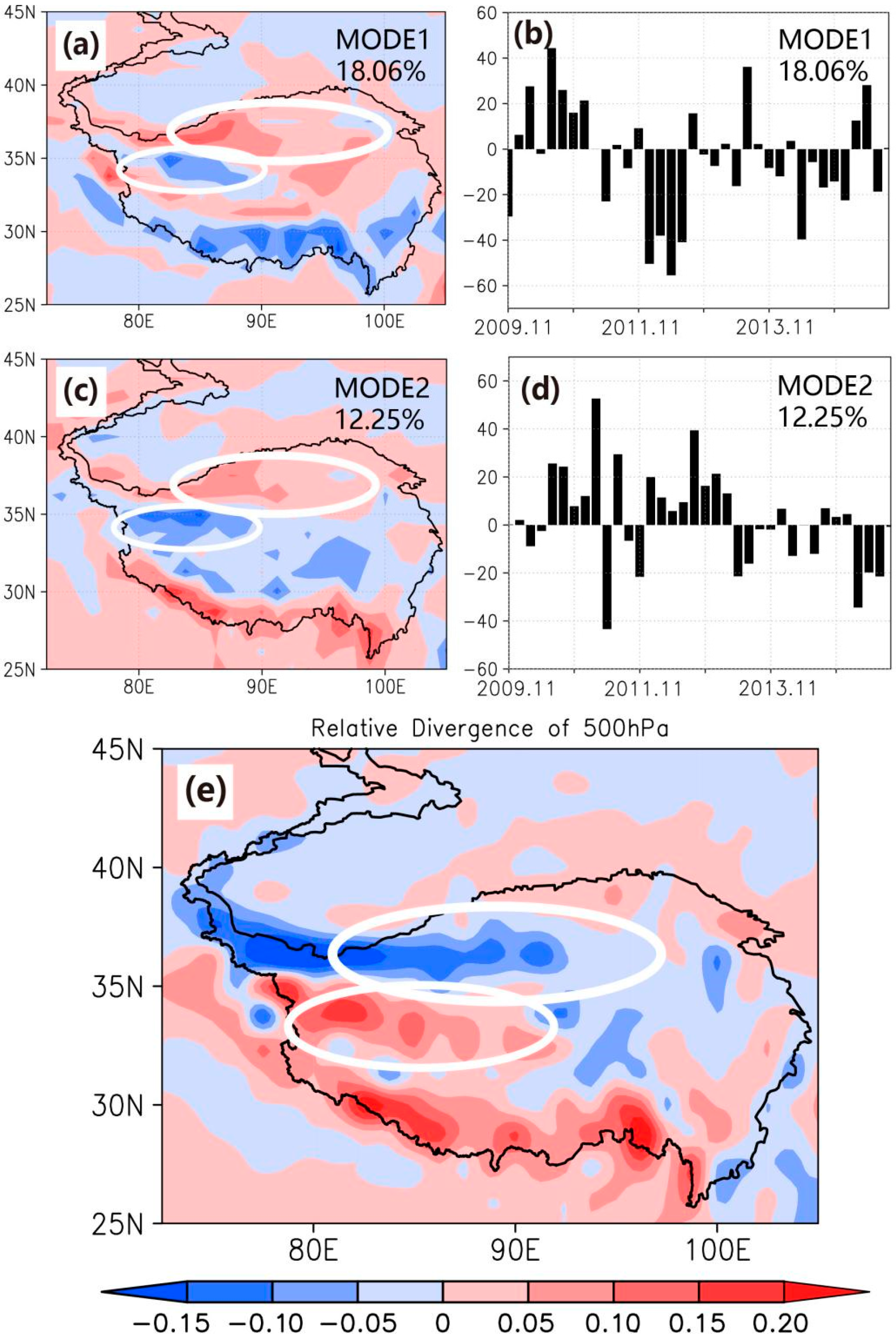
Figure 4 shows the EOFs of the anomaly field and the mean field of the relative divergence at 500 hPa over the Tibetan Plateau from November to next April 2009–2014.
It can be found that there was little difference in the explained variances of the first two modes, which can both be regarded as relatively significant modes. Compared with the mean field (
Figure 4e), it can be seen that the divergence anomaly in the first mode was almost completely opposite to the average divergence, that is, there were negative anomalies in the Himalayan Mountains (on the south) and the central plateau, and positive anomalies in the southern Tibetan Valley (on the north of the Himalayan Mountains), the north and the mid-eastern part of the plateau (
Figure 4a). The time coefficients indicated that this feature was more obvious from the winter of 2009 to the spring of 2010, and the opposite feature was found for the period of the 2011 winter to 2012 spring (
Figure 4b). In the second mode, there was a positive anomaly in the Himalayan mountains, a negative anomaly in the main region of the plateau, and a positive anomaly in the northern part (
Figure 4c). With the time coefficients also taken into consideration, this feature was obvious in the spring and winter of 2010, and in the winter of 2011 to the winter of 2012 (
Figure 4d). In general, in 2009 and 2012, when the drought was severe, divergence anomalies of the main part of the plateau (including the central plateau and the northern mountains) were obviously opposite to the mean field (white circles in
Figure 4). In other words, in the period of severe drought in Southwest China, the relative divergence field of 500 hPa over the Tibetan Plateau tended to weaken, no matter whether it was convergence or divergence.
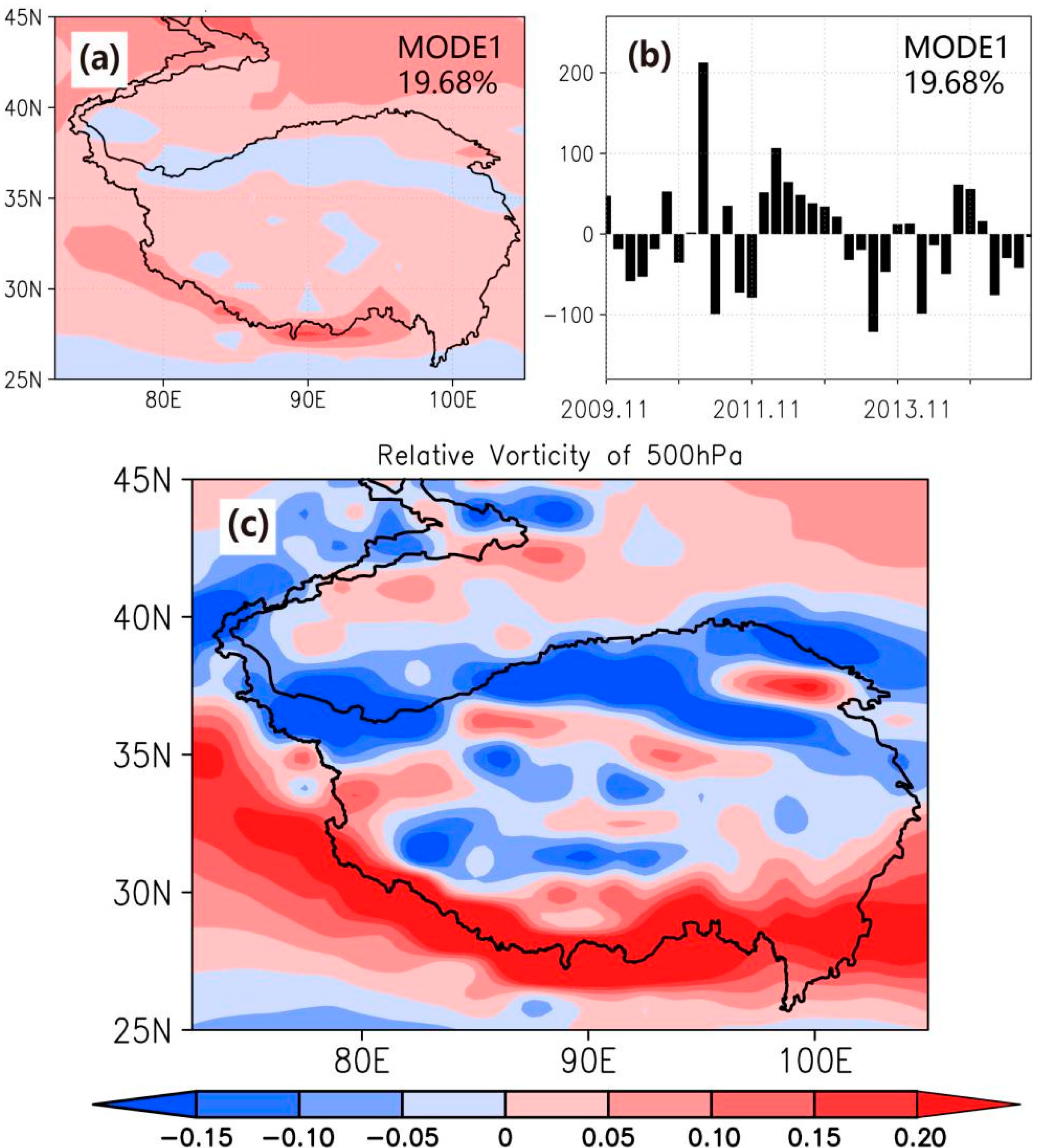
The EOF of the anomaly field and the mean field of the relative vorticity at 500 hPa over the Tibetan Plateau from November to next April 2009–2014 were shown in
Figure 5. The first two modes have passed the North Test [
32].
It can be seen that the plateau vorticity anomaly at 500 hPa was mainly positive, with the positive vorticity strengthening and the negative vorticity weakening, which was contrary to the large-area negative vorticity in the mean field (
Figure 5c). In other words, the relative vorticity field near the plateau surface also tended to weaken in the winter season.
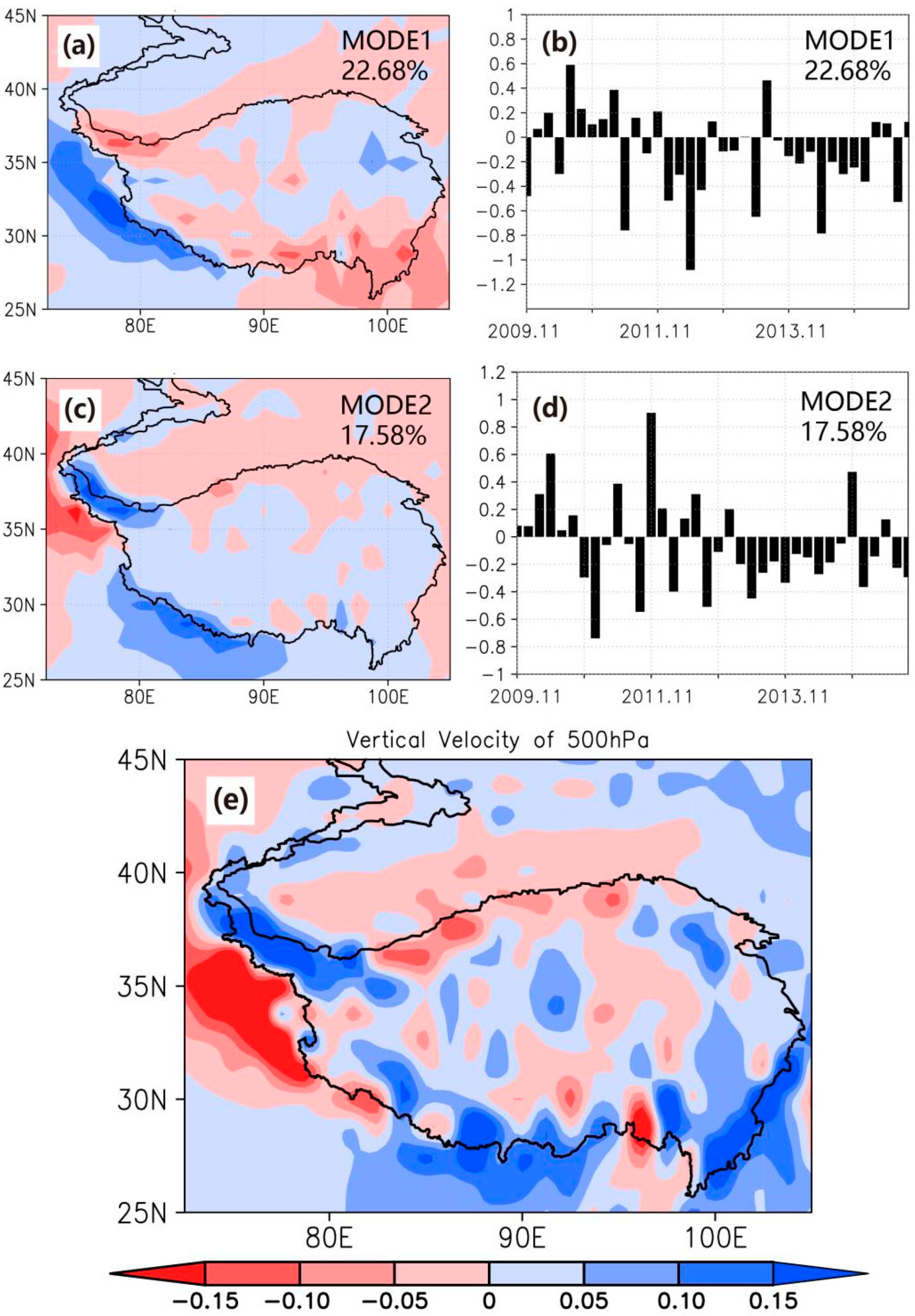
Finally, the EOF of the anomaly field and the mean field of the vertical wind component velocity at 500 hPa over the Tibetan Plateau from November to next April 2009–2014 was shown in
Figure 6.
The main vertical movement over the Tibetan Plateau in winter was the downdraft caused by both thermal and dynamic action, which can also be reflected in the mean field (
Figure 6e). The first and the second EOF mode, both with significant explained variances (22.68% and 17.58%, respectively), showed that the main region of the Tibetan Plateau was negative anomalous with dominant negative time coefficients, that is, during the drought in Southwest China, the downdraft over the Tibetan Plateau had an abnormal tendency to be weaker than the average state.
3.2. The Flow of Westerly Wind and the Intersection of Cold and Warm Air
As mentioned above, Southwest China is alternatively controlled by winter and summer monsoons, and the distribution of precipitation is uneven among the seasons. The rainy season is formed under the influence of the summer monsoon system, and the dry season is formed under the influence of the winter monsoon system [
33]. Until now, it has been generally believed that the main precipitation system in winter in Southwest China is the Kunming quasi-stationary front (in the southwest) and the South China quasi-stationary front (in the southeast). The South China quasi-stationary front is located in the east of Southwest China and only affects part of Guangxi. In winter, the westerlies are blocked by the Tibetan Plateau, which they bypass. The northern branch forms a ridge of high pressure, which merges with the cold air from the north and moves southward under the influence of the anticyclone formed by the thermal effect over the Tibetan Plateau. Then, it is blocked again by the Yunnan–Guizhou Plateau. The southern branch bypasses the Tibetan Plateau to form the south trough near the Bay of Bengal, and merges with the warm current towards the north. The cold and dry continental air flowing along the Northern Slope of Yunnan–Guizhou Plateau intersects with the warm air between Kunming and Guiyang, forming the Kunming quasi-stationary front. The weather on two sides of the front is quite different: on the cold air (northeast) side of the Kunming quasi-stationary front, Guizhou, Sichuan, Chongqing and other places are wet with rain (or snow) from time to time, while Yunnan and other areas on the warm (southwest) side are controlled by the warm air mass, hence are sunny with less rain. Once the cold air is strong and the quasi-stationary front moves westward and southward crossing over the mountains, there may be more rainy days in winter in Yunnan [
20,
21].
During the drought events in Southwest China from 2009 to 2014, the convergence of the dynamic field in the upper level and the divergence in the lower level of the Tibetan Plateau both weakened, the absolute value of relative vorticity in the lower level was smaller, and the downdraft was also weaker. It can be concluded that during the drought in Southwest China, the high-pressure anticyclone formed by the thermal effect over the Tibetan Plateau tended to diminish.
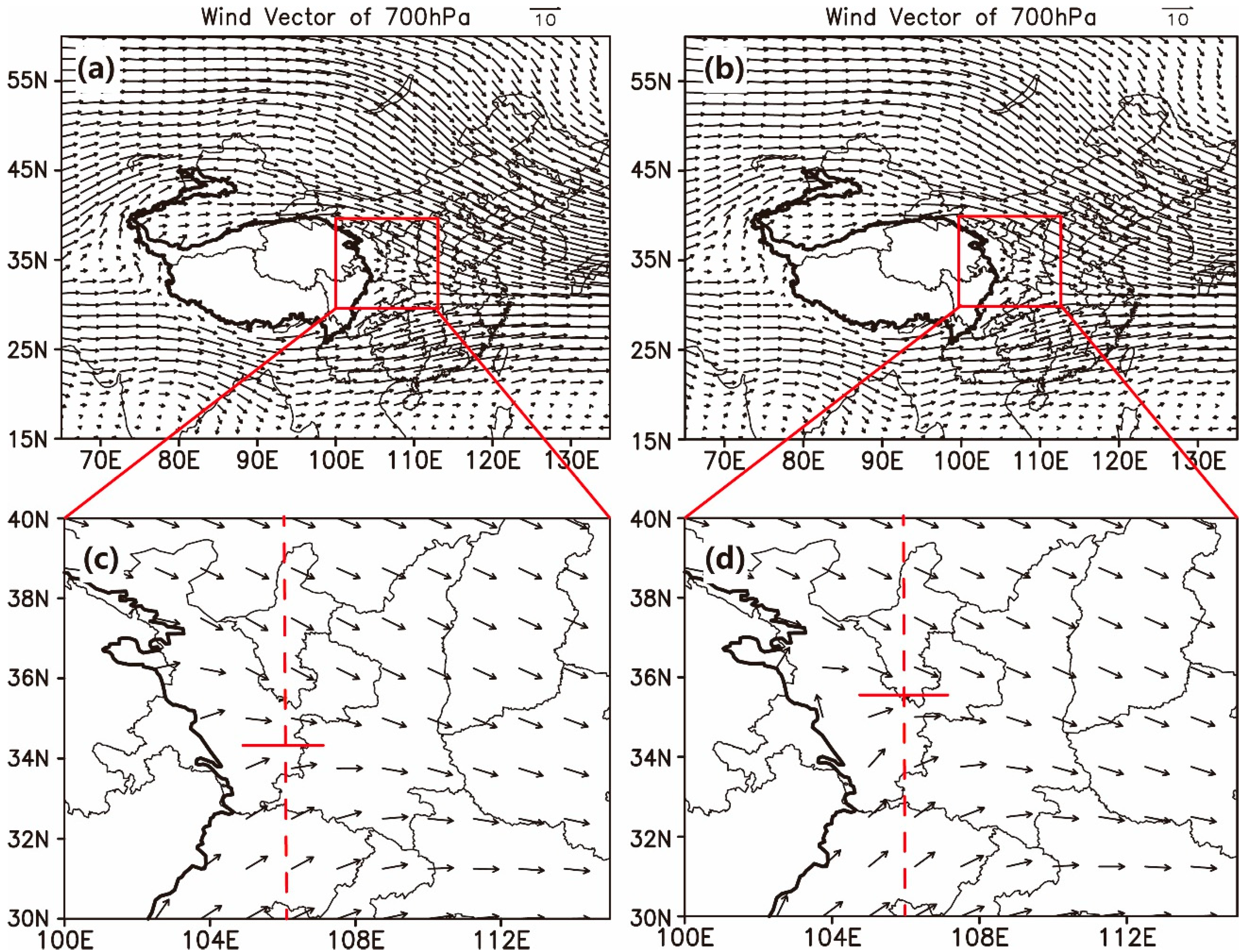
When the clockwise circulation of the anticyclone slowed down, the intensity of the northern and southern air flows formed by the westerlies meeting the plateau terrain would also change. The flow on the northeast towards the south weakened, while the flow on the southeast towards the north strengthened. By comparing the mean wind field of the dry season of 2009–2014 with that of 1960–2019 (
Figure 7), it can be found that at about 106°E at 700 hPa (red dotted lines), at the mean field of 1960–2019 (a) and (c), the latitude where the northward and southward branch airflow met on the east side of the Tibetan Plateau was lower than 35°N. However, under the mean state during the drought event in Southwest China (b) and (d), the intersection of northward and southward branch airflows exceeded 35°N, which was about 1° north of that in the average state.
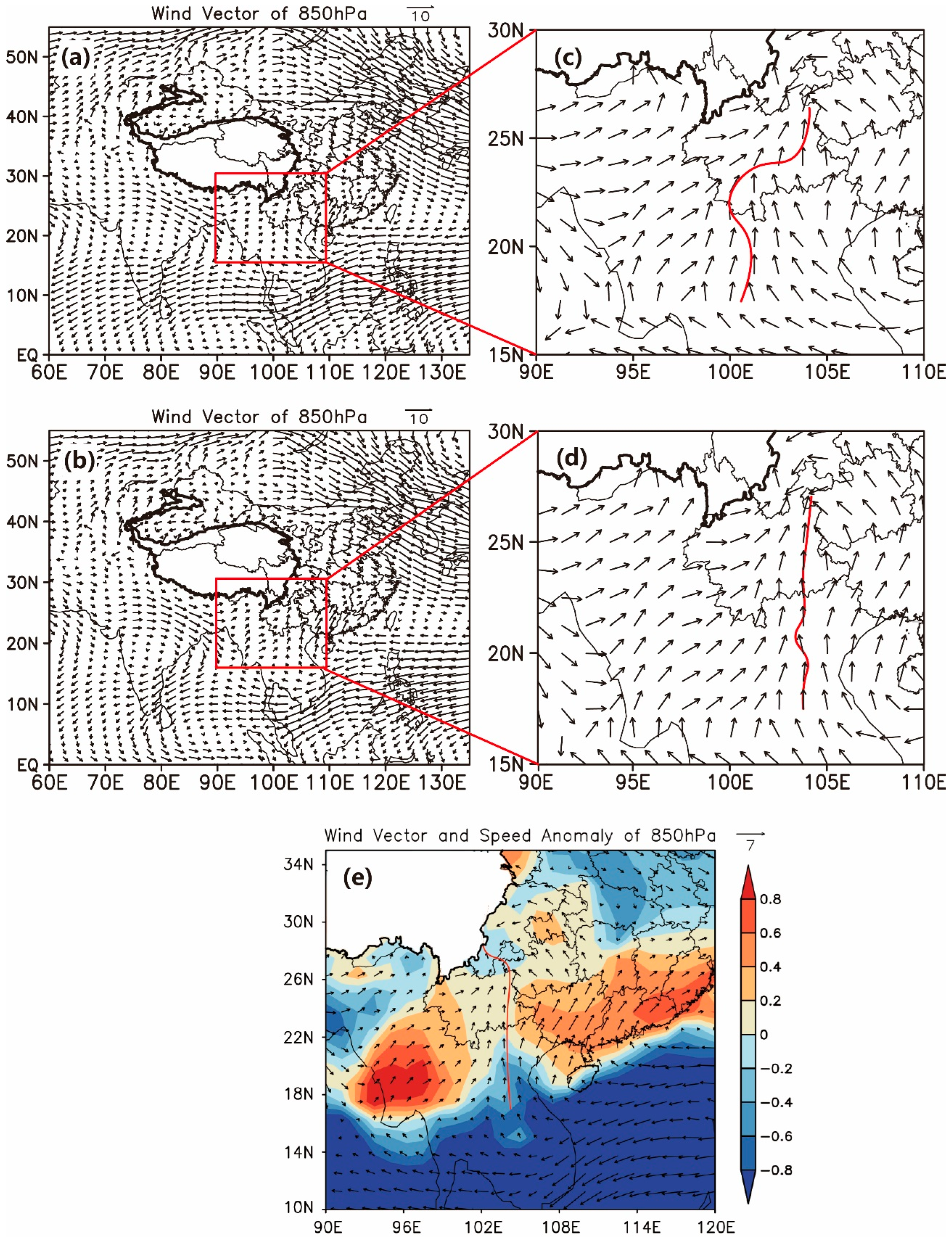
At 850 hPa where warm and cold air often intersect (see
Figure 8), there were two air currents controlling the Southwest China climate: one was the southeast air flow coming from the Pacific Ocean, and the other was the southwest current. Part of the latter was from the dry continent in central Asia, and the other part was the current turned from the southeast Pacific trade winds. According to the 1960–2019 average, the east and west wind converged near 101°E at around 20°N, while during the 2009–2014 drought, the convergence line moved eastward to near 104°E, with a gap of 2–3°. As can be seen from
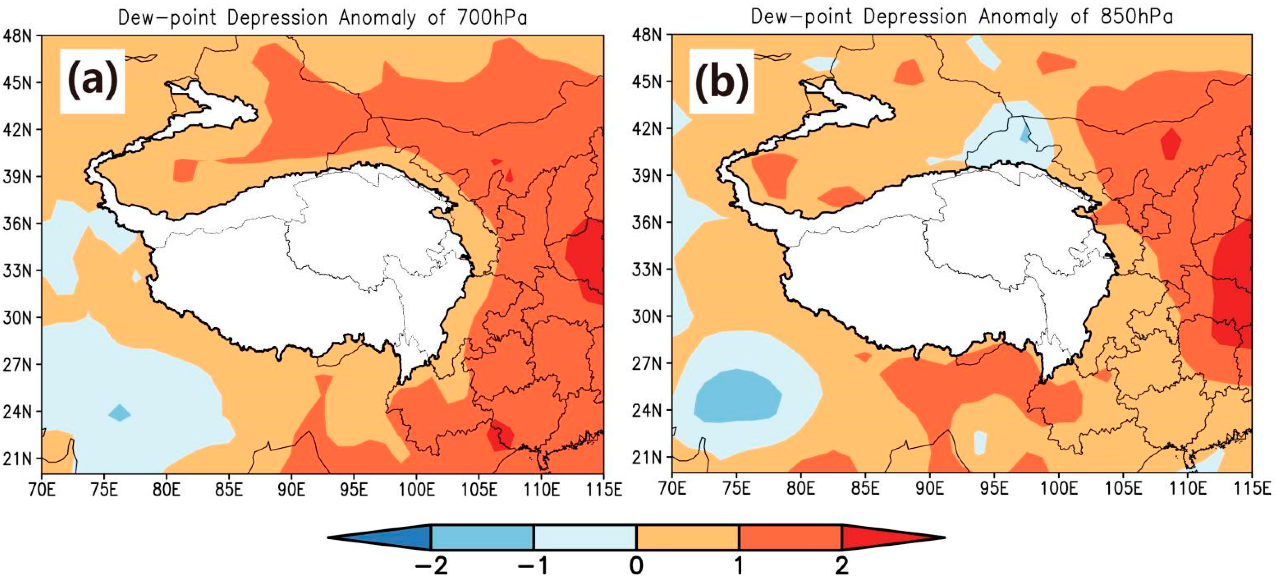
Figure 8e, on the west side of the convergence line, there was a strong positive abnormal center of southwest wind speed, while on the east side, there was also a southwest wind anomaly where the easterly (weaker) air wind flow used to be (which means a weaker east wind flow), indicating that the strong dry west wind pushed the southeast wind from the Pacific to the east, resulting in the reduction in water vapor content in Southwest China. This was also confirmed by the abnormal increase in the dew point depression (see
Figure 9). During the drought event, the dew point depression in the region at 700 hPa and 850 hPa was 0.5–1 °C higher than the 1960–2019 dry season average. It could be demonstrated that the difference between the dew point temperature and the actual temperature during this period was larger, and the relative humidity was lower.
3.3. The Regression Analysis of Dynamic Anomaly of the Tibetan Plateau and Precipitation in Southwest China
As long as we confirmed that the dynamic field anomalies on the Tibetan Plateau were inherently related to the precipitation in Southwest China, it was reasonable to try a quantitative method to measure this relationship. Here, we chose regression. It was found that each dynamic field element had similar distribution characteristics at 600 hPa to 400 hPa (low level) and 300 hPa to 100 hPa (high level), respectively. Therefore, a total of six dynamic field elements at 500 hPa and 200 hPa levels were selected in the regression analysis. They were relative divergence, relative vorticity and vertical velocity at 500 hPa and 200 hPa, respectively. Each factor was averaged from November to April (the months affected by winter monsoon), and then EOF analysis with 59 years of time series from 1960 to 2019 was conducted. At last, unary and multiple (up to four variables) linear regression analyses were conducted between the time coefficients of EOF and the anomaly percentage of precipitation average of all stations in the same period in Southwest China. All the below-listed regression equations have passed the F-test.
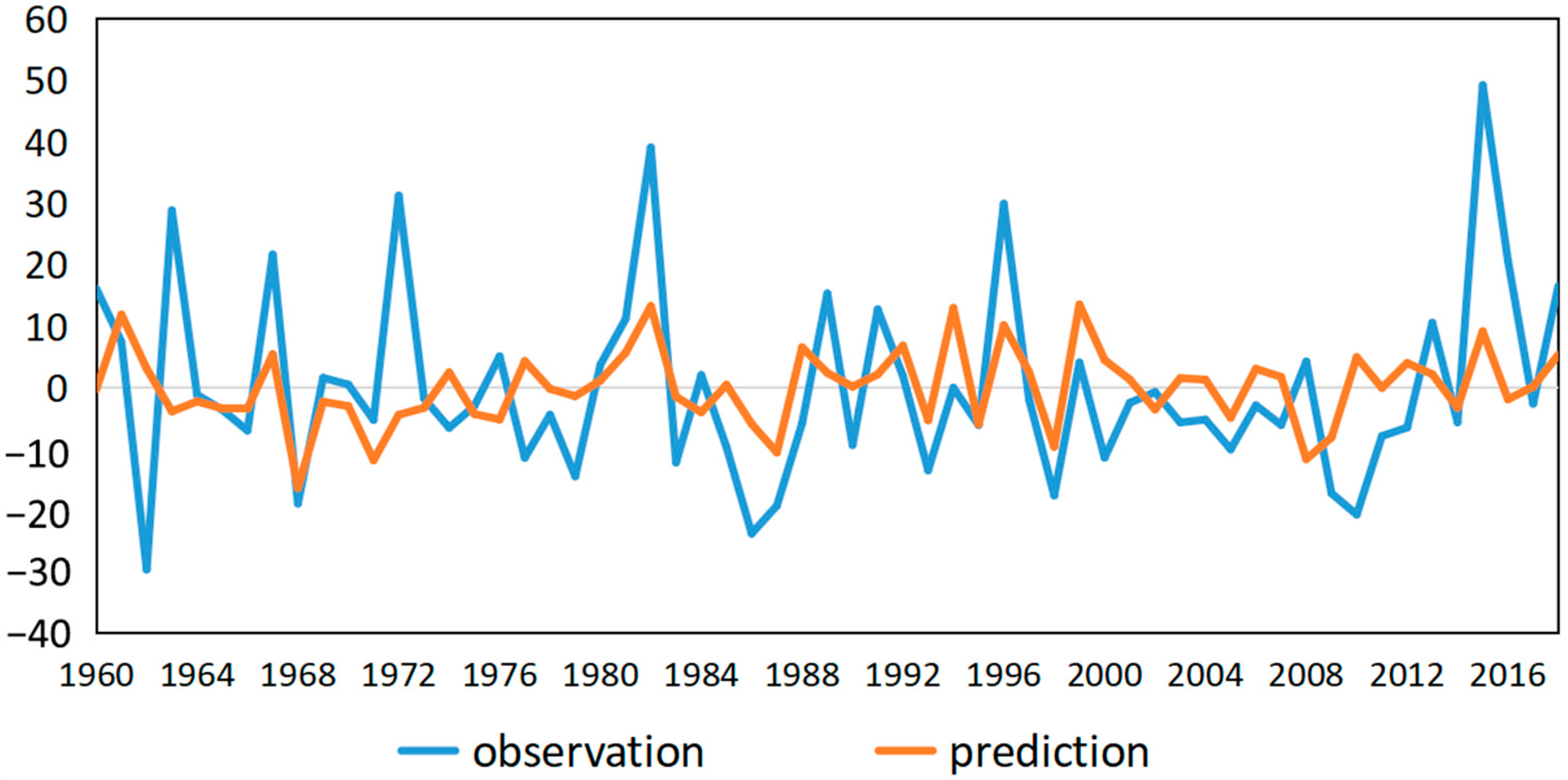
Among all the tested linear regression equations, the one that worked best was the following binary regression equation:
In the formula, y denotes the forecast value of precipitation anomaly percentage, denotes the EOF time coefficient of 500 hPa relative vorticity anomaly in 59 years, and denotes the EOF time coefficient of 500 hPa relative divergence anomaly in 59 years.
Next, the time coefficients were substituted into the regression equation to obtain the forecast values; the comparison between the forecast value and the observed value is described below. The Mean Absolute Error (MAE) of the equation was 0.106, and the Root Mean Square Error (RMSE) was 0.138, both of which were acceptable (when the difference between the maximum and the minimum of the observation was about 0.79). The Pearson correlation coefficient between the forecast value and the observed value was 0.408, which exceeded the critical value of correlation coefficient 0.336 (degree of freedom: N − M − 1 = 56) at the significance level of 0.01, which means passing the reliability test with 99%.
It can be seen from
Figure 10 that the regression equation could predict the overall trend and most peak and valley situations, while the absolute value prediction of some peak and valley values was not accurate.
We also made further attempts. In unitary linear regression analysis, the best result was the equation with relative vorticity at 500 hPa, whose correlation coefficient was 0.368 between the forecast value and the observed value, and it was not as accurate as the binary equation in the prediction of peak and valley values. For the equation with four unknowns, when the value was close to 0, the difference of the quaternionic regression equation was larger than that of the binary equation, and it was more prone to qualitative forecast errors, which had a great influence on the accuracy of the forecast.
4. Discussion
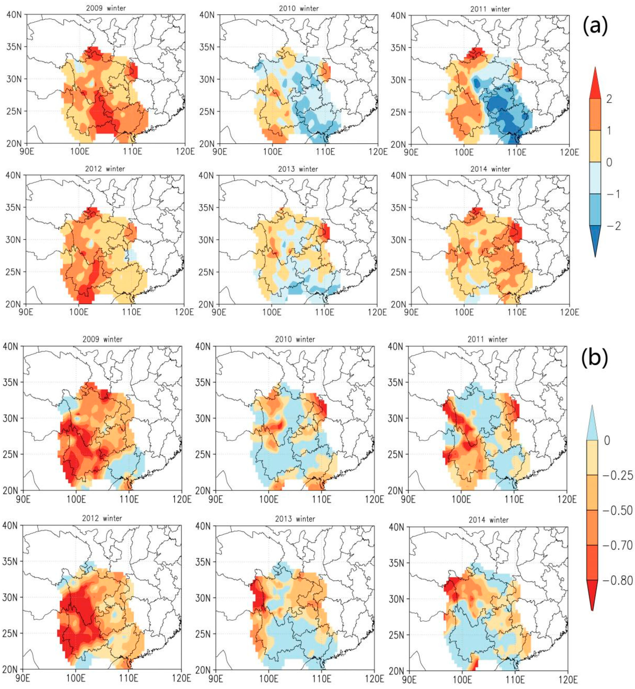
When comparing the surface temperature field (see
Figure 11a) with precipitation anomalies (see
Figure 11b) during drought events in Southwest China, it was noticed that the areas with positive temperature anomalies coincided greatly with the areas with drought, and the boundary of the drought was close to the boundary of positive and negative temperature anomalies. In 2009 and 2012, when the winter droughts were quite severe, almost the entire area of Southwest China experienced warmer temperatures than usual. There were also quite high Pearson correlation coefficients between two groups of grid data, such as 0.222 for 2010 and 0.427 for 2013 (with 818 grids) at the significance level of 0.001. All these observations indicate that the location changes of cold and warm air masses did have a strong relationship with precipitation in Southwest China, which is consistent with our results.
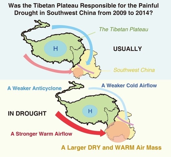
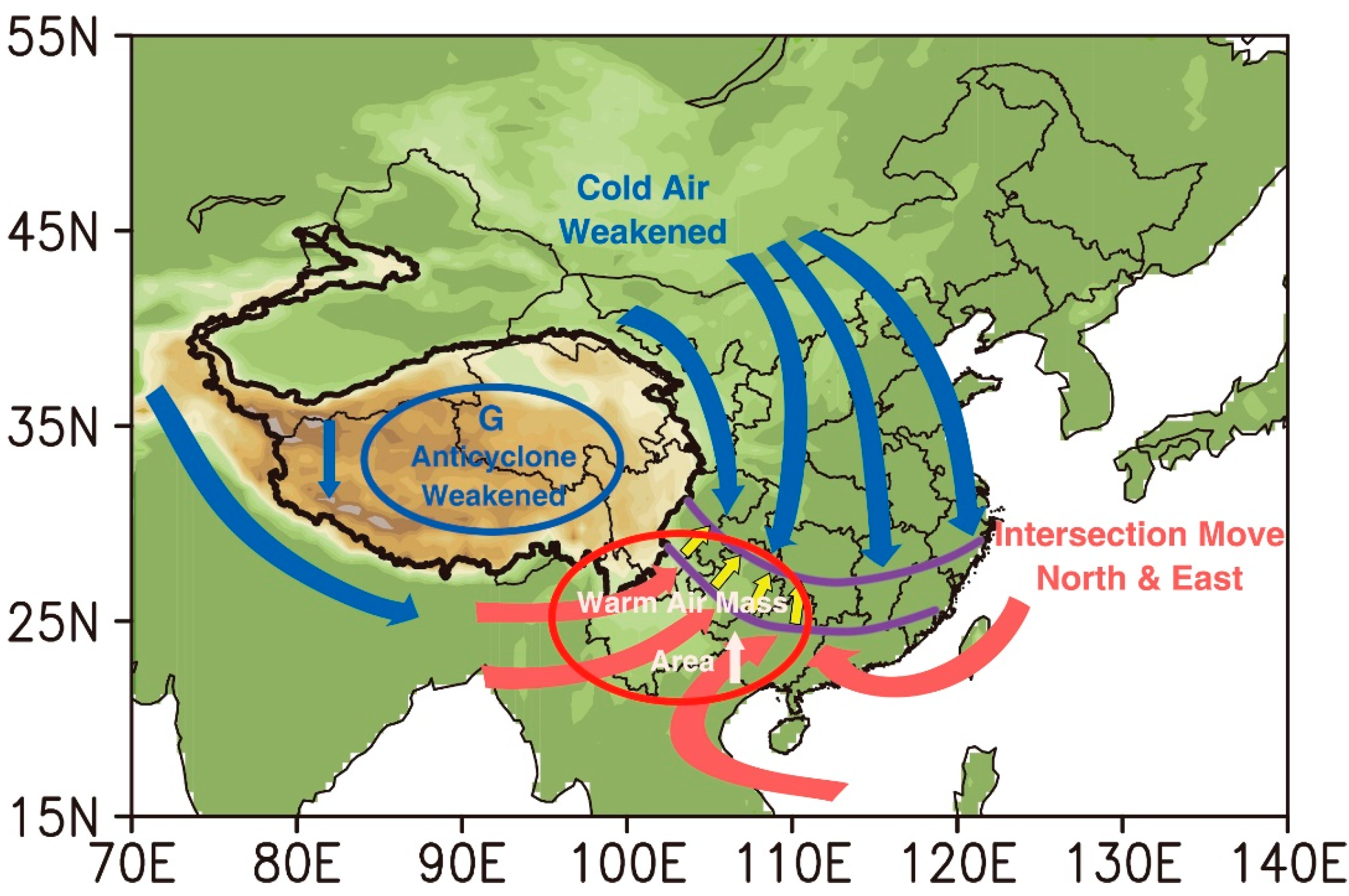
To summarize the above-listed results, we raised a conceptual model of the dynamic effect influencing drought in Southwest China (see
Figure 12). It could be inferred that during the drought events, the momentum of cold air moving southward from the north weakened, while the westerly wind from the dry region of Central Asia was strong in the south. The convergence area of cold and warm air was more to the north and east than usual, and the area controlled by warm air mass in the southwest was larger, which was not conducive to precipitation.
To some extent, the above result is also in line with some previous research. A few studies have attributed this drought event to the negative phase of the Arctic Oscillation [
34,
35,
36,
37,
38,
39], which caused the cold air in East Asia to move through an eastern route, so that less air flows southwards along the plateau, consistent with that illustrated in this model.
Through the EOF analysis and regression analysis above, it has been found that during the same period of drought in Southwest China, the anticyclone was abnormally weak over the Tibetan Plateau, and its influence mechanism on drought in Southwest China was discussed. However, there are still other problems worthy of additional research.
Firstly, the reasons for the weakening of the anticyclone over the Tibetan Plateau in winter deserve further investigation. The reasons may include abnormal circulation caused by global warming, that is, abnormal weakening of the sinking branch of Hadley circulation or Ferrer circulation in the subtropical zone [
40]; the thermal anomaly of the Tibetan Plateau itself, that is, the higher temperature at a low level, which may be caused by global warming and the change of snow-covered area [
41].
In addition, it is expected that more ground and upper air observation stations will be built on the Tibetan Plateau and its adjacent areas along with the regular collection of more complete data, so that we can obtain a more accurate prediction of drought events in Southwest China.
5. Conclusions
The westerlies are separated into two branches, i.e., the northern branch and southern branch, when encountering the Tibetan Plateau. These two branches have great impacts on the weather and climate of the area where they pass, and then converge on the eastern side of the plateau, affecting the local distribution of temperature and rainfall. However, there have been few studies on how the Tibetan Plateau influence these two branches of the westerlies. It has not been clear whether there was a relationship between the Tibetan Plateau, the branches of the westerlies and the severe drought event that happened in Southwest China in 2009–2014. In addition, most previous research did not regard this continuous drought as a whole, as there was more specific work about the drought in one single year. This paper tried to deal with the problems above using some statistical methods such as EOF analysis and regression analysis. The following conclusions have been drawn:
(1) Most areas in Southwest China experienced different degrees of continuous abnormal drought in spring, autumn, and especially winter, between 2009 and 2014.
(2) The relative divergence, relative vorticity and vertical velocity at a low level over the Tibetan Plateau all showed the abnormal characteristics of a smaller absolute value of elements from November to April in the period of 2009–2014. Namely, during the drought in Southwest China, the downdraft over the Tibetan Plateau and the anticyclone both weakened.
(3) When the anticyclone weakened over the Tibetan Plateau in the winter season, the cold air from the northern branch of the westerly weakened, such that the cold air flowing southward on the northeast of the plateau weakened dwindled. In the south, the westerly wind from the arid region of Central Asia strengthened, and the intersection of cold and warm air moved eastward and northward, so that a larger area of Southwest China was controlled by a dry and warm air mass, which was not conducive to precipitation.
(4) A binary linear regression forecast model for precipitation in Southwest China was established: , where y denotes the forecast value of precipitation anomaly percentage, denotes the EOF time coefficient of 500 hPa relative vorticity anomaly from 1960 to 2019, and denotes the EOF time coefficient of 500 hPa relative divergence anomaly from 1960 to 2019. The correlation coefficient between the forecast value and the observed value was 0.408, passing the reliability test with 99%.


