

An Effective Deep Learning Model for Monitoring Mangroves: A Case Study of the Indus Delta

Abstract
:
1. Introduction
2. Materials
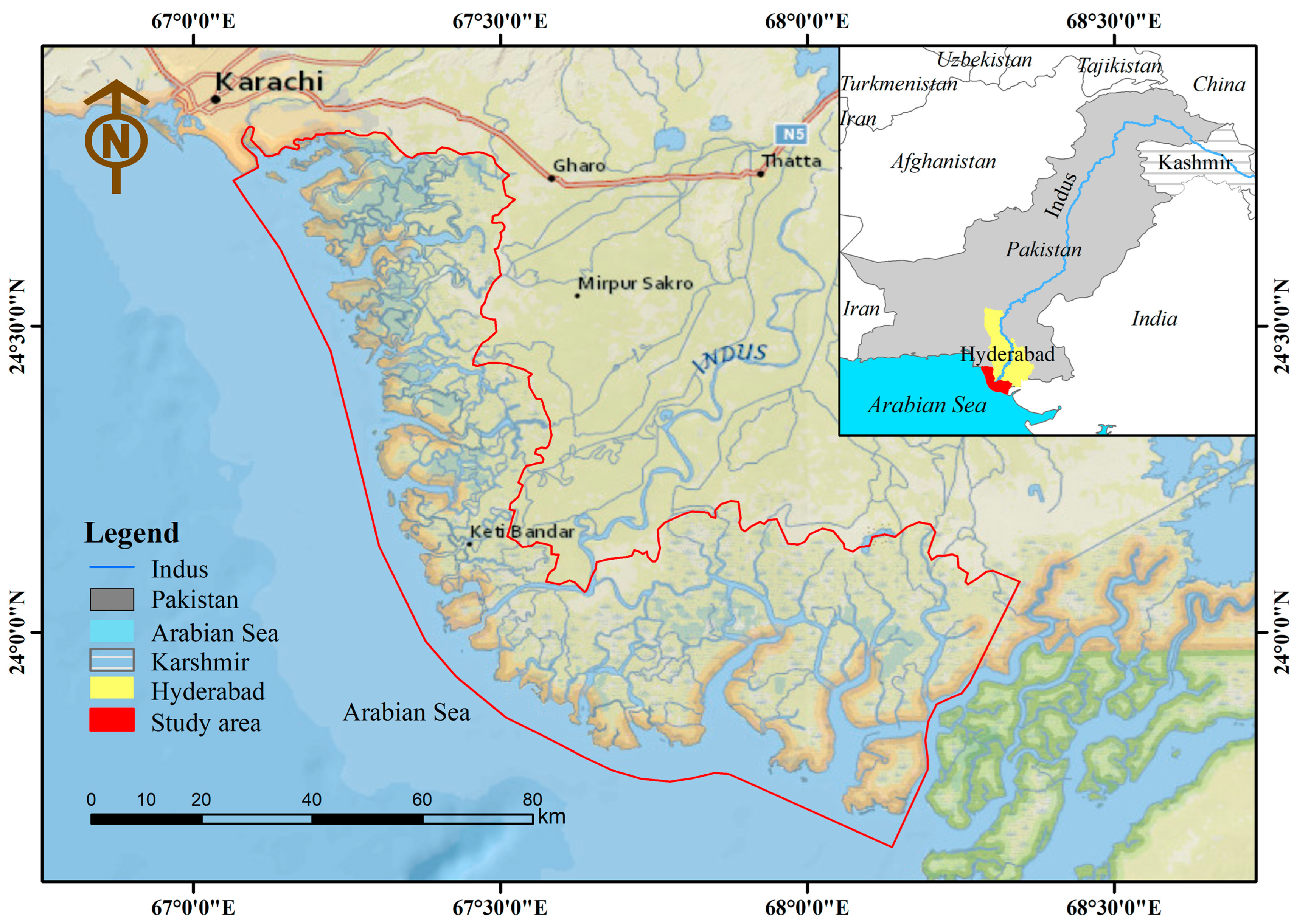
2.1. Study Area
2.2. Data
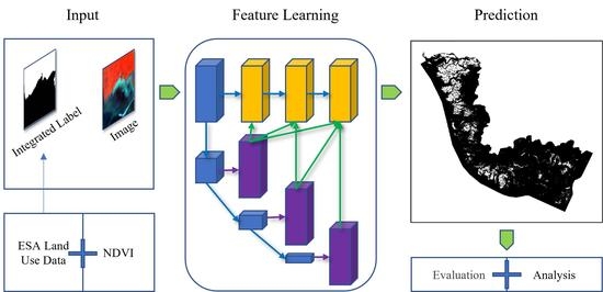
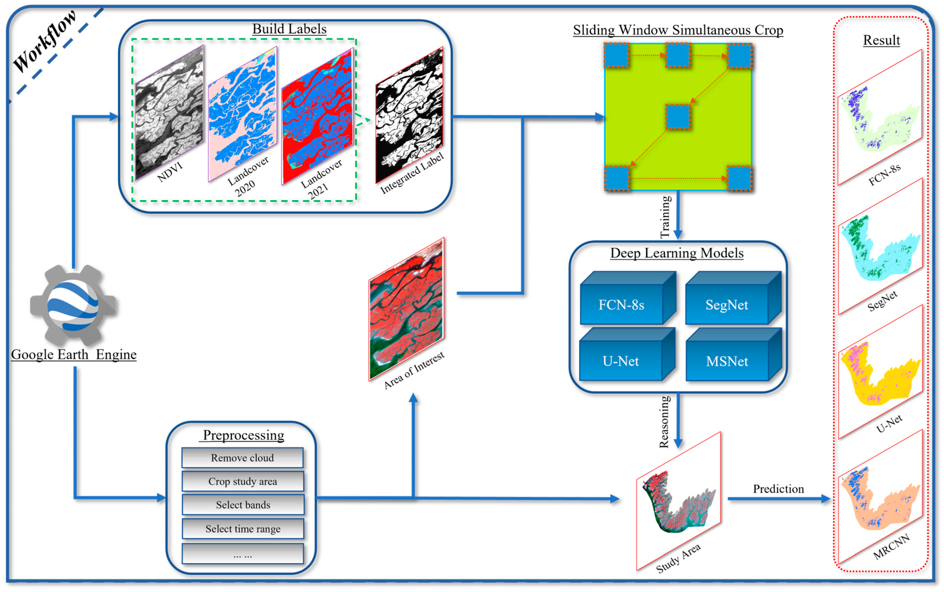
3. Methods
3.1. Label Building
3.2. Deep Learning Models
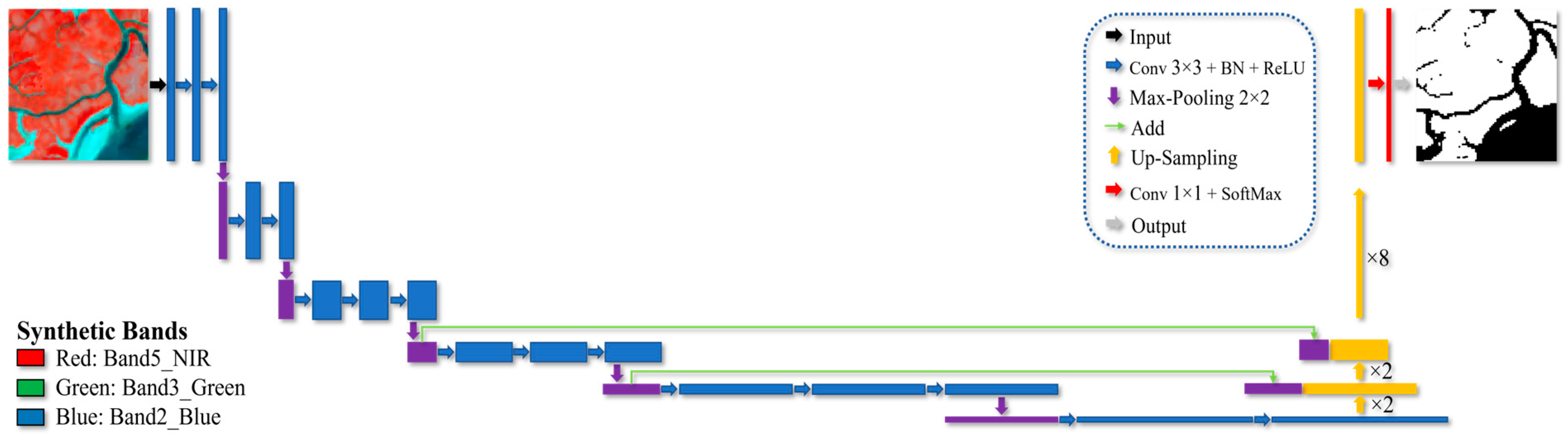
3.2.1. FCN-8s
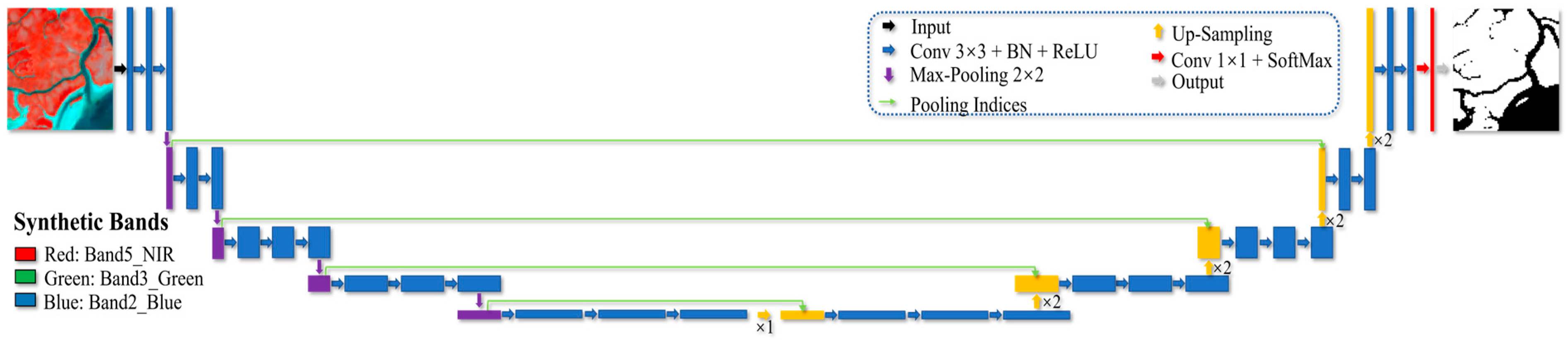
3.2.2. SegNet
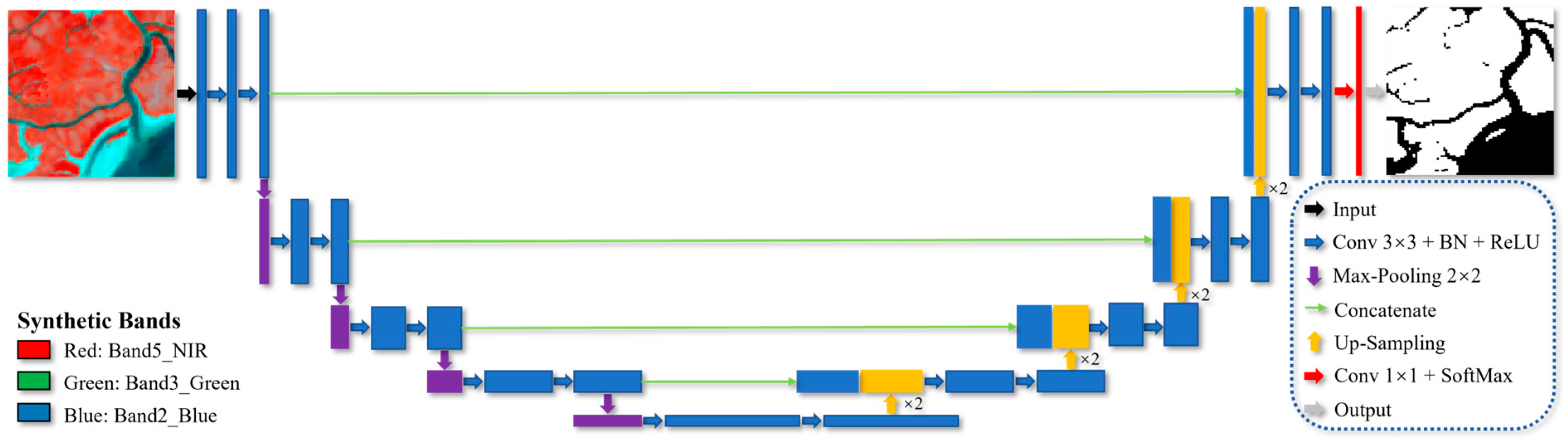
3.2.3. U-Net
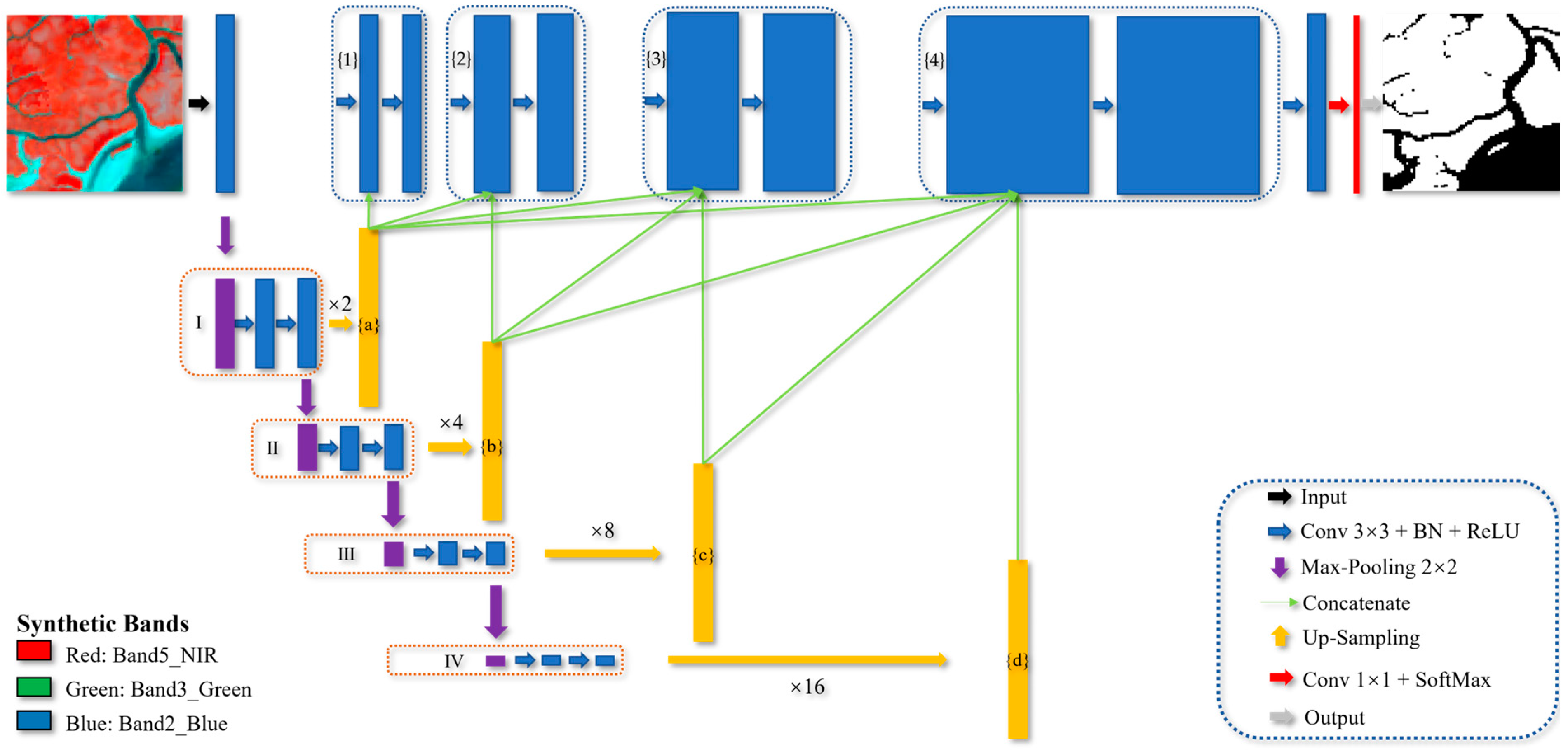
3.2.4. MSNet
3.3. Evaluation Metrics
4. Results
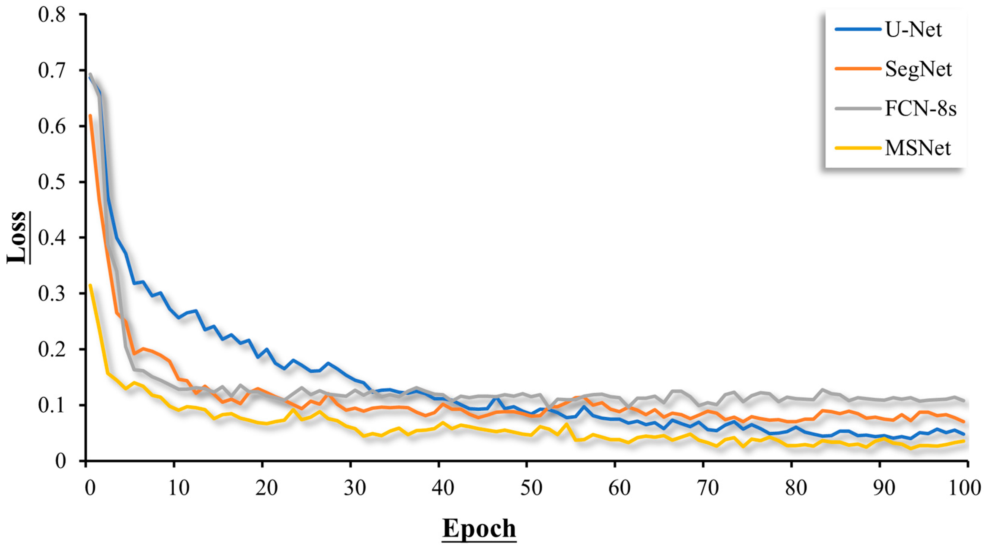
4.1. Performance of Models
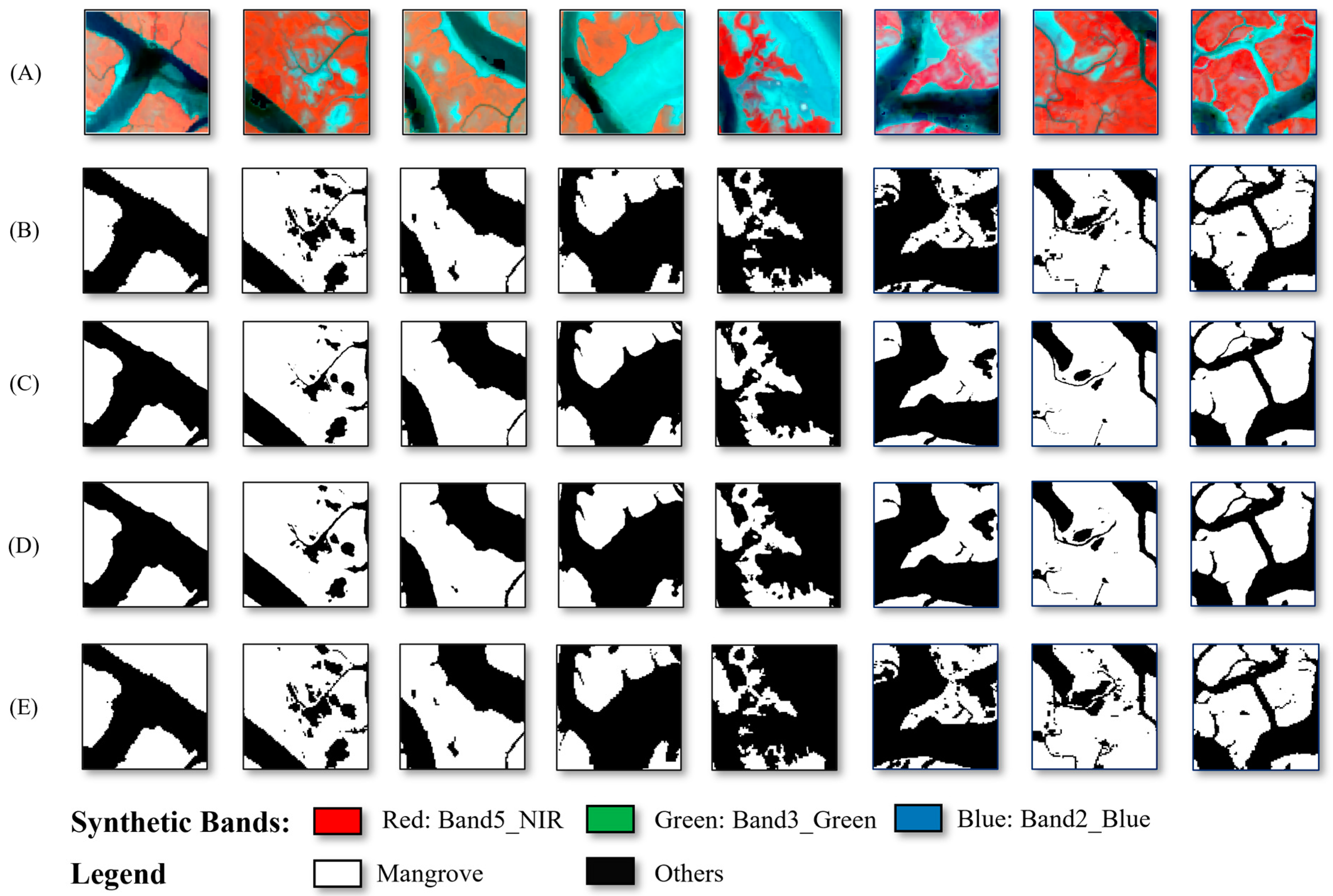
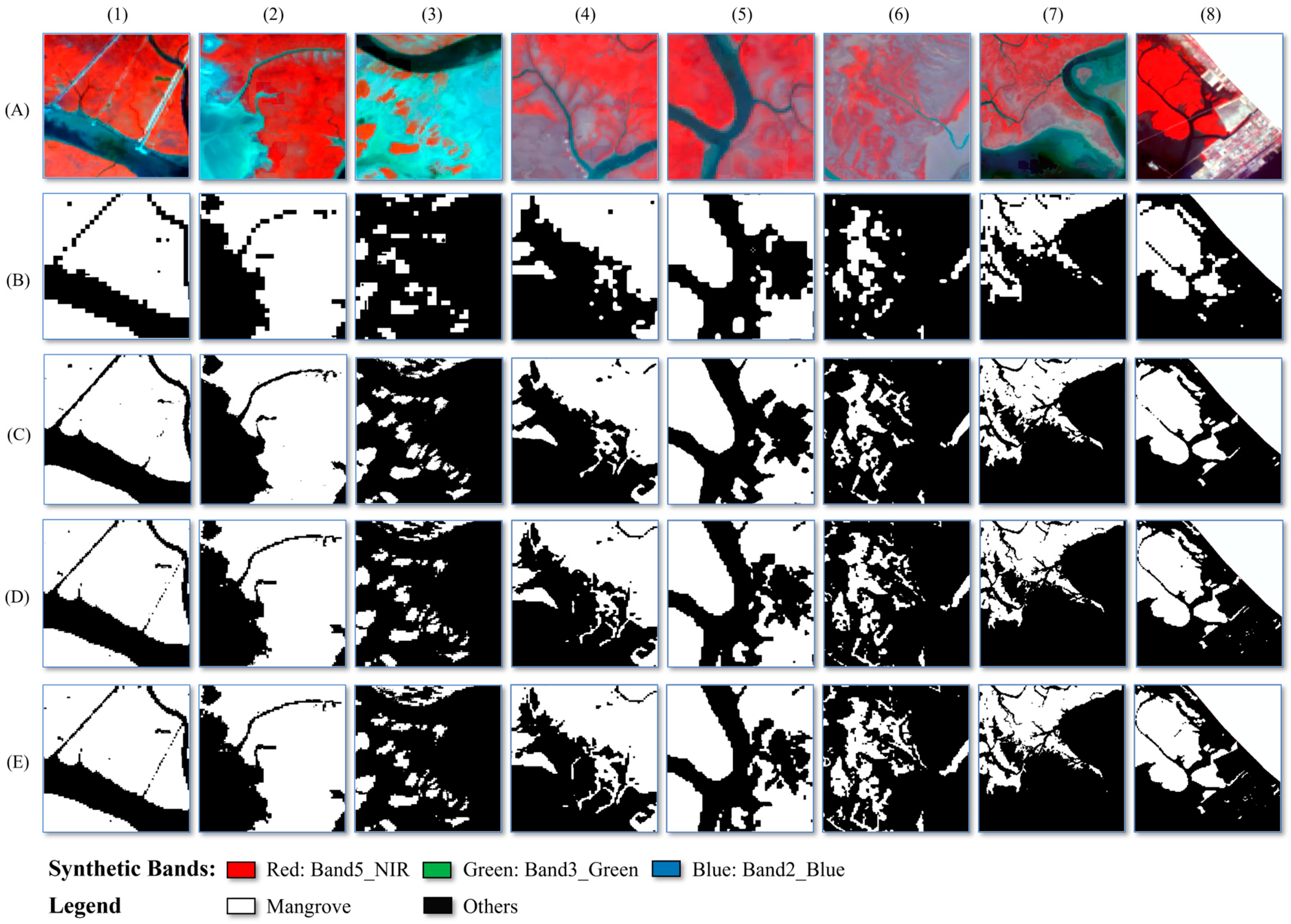
4.2. Extraction Results of Mangroves
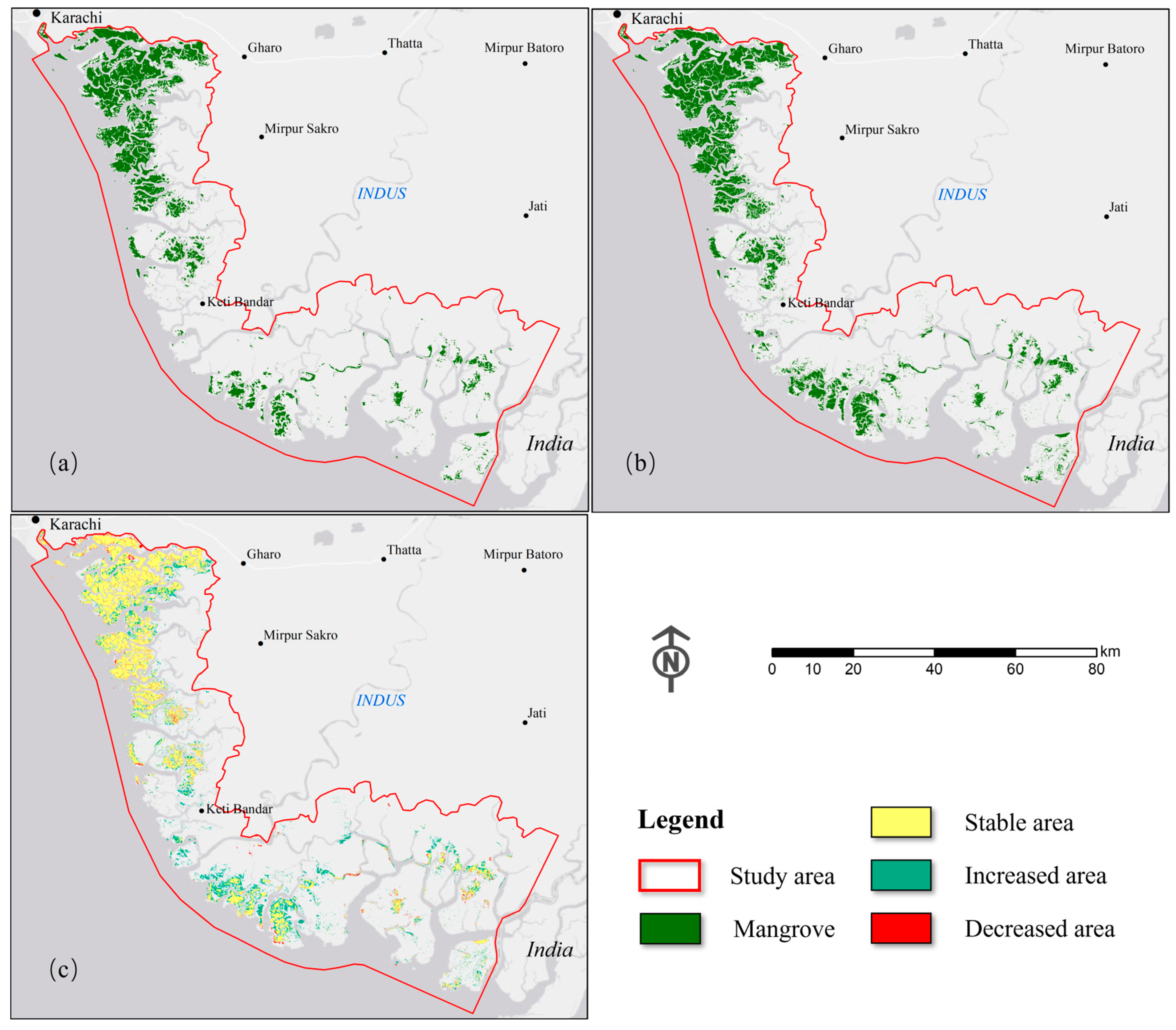
4.3. Spatial Variation of Mangroves
5. Discussion
6. Conclusions
Author Contributions
Funding
Data Availability Statement
Acknowledgments
Conflicts of Interest
References
- Wang, L.; Sousa, W.P.; Gong, P.; Biging, G.S. Comparison of IKONOS and QuickBird Images for Mapping Mangrove Species on the Caribbean Coast of Panama. Remote Sens. Environ. 2004, 91, 432–440. [Google Scholar] [CrossRef]
- Agaton, C.B.; Collera, A.A. Now or Later? Optimal Timing of Mangrove Rehabilitation under Climate Change Uncertainty. For. Ecol. Manag. 2022, 503, 119739. [Google Scholar] [CrossRef]
- Han, X.; Fu, D.; Ju, C.; Kang, L. 10-M Global Mangrove Classification Products of 2018–2020 Based on Big Data. Sci. Data Bank 2021. [Google Scholar] [CrossRef]
- Murdiyarso, D.; Purbopuspito, J.; Kauffman, J.B.; Warren, M.W.; Sasmito, S.D.; Donato, D.C.; Manuri, S.; Krisnawati, H.; Taberima, S.; Kurnianto, S. The Potential of Indonesian Mangrove Forests for Global Climate Change Mitigation. Nat. Clim. Change 2015, 5, 1089–1092. [Google Scholar] [CrossRef]
- Goldberg, L.; Lagomasino, D.; Thomas, N.; Fatoyinbo, T. Global Declines in Human—Driven Mangrove Loss. Glob. Change Biol. 2020, 26, 5844–5855. [Google Scholar] [CrossRef]
- Memon, J.A.; Thapa, G.B. Explaining the de Facto Open Access of Public Property Commons: Insights from the Indus Delta Mangroves. Environ. Sci. Policy 2016, 66, 151–159. [Google Scholar] [CrossRef]
- Amir, S.A.; Siddiqui, P.J.A.; Masroor, R. Finfish diversity and seasonal abundance in the largest arid mangrove forest of the Indus Delta, Northern Arabian Sea. Mar. Biodivers. 2018, 48, 369–1380. [Google Scholar] [CrossRef]
- Giri, C.; Long, J.; Abbas, S.; Murali, R.M.; Qamer, F.M.; Pengra, B.; Thau, D. Distribution and Dynamics of Mangrove Forests of South Asia. J. Environ. Manag. 2015, 148, 101–111. [Google Scholar] [CrossRef]
- Irum, M.; Abdul, H. Constrains on mangrove forests and conservation projects in Pakistan. J. Coast. Conserv. 2012, 16, 51–62. [Google Scholar] [CrossRef]
- Friess, D.A.; Rogers, K.; Lovelock, C.E.; Krauss, K.W.; Hamilton, S.E.; Lee, S.Y.; Lucas, R.; Primavera, J.; Rajkaran, A.; Shi, S. The State of the World’s Mangrove Forests: Past, Present, and Future. Annu. Rev. Environ. Resour. 2019, 44, 89–115. [Google Scholar] [CrossRef] [Green Version]
- Li, H.; Wang, C.; Cui, Y.; Hodgson, M. Mapping Salt Marsh along Coastal South Carolina Using U-Net. ISPRS J. Photogramm. Remote. Sens. 2021, 179, 121–132. [Google Scholar] [CrossRef]
- Matsushita, B.; Yang, W.; Chen, J.; Onda, Y.; Qiu, G. Sensitivity of the Enhanced Vegetation Index (EVI) and Normalized Difference Vegetation Index (NDVI) to Topographic Effects: A Case Study in High-Density Cypress Forest. Sensors 2007, 7, 2636–2651. [Google Scholar] [CrossRef] [Green Version]
- Houborg, R.; Soegaard, H.; Boegh, E. Combining Vegetation Index and Model Inversion Methods for the Extraction of Key Vegetation Biophysical Parameters Using Terra and Aqua MODIS Reflectance Data. Remote. Sens. Environ. 2007, 106, 39–58. [Google Scholar] [CrossRef]
- Manna, S.; Raychaudhuri, B. Mapping distribution of Sundarban mangroves using Sentinel-2 data and new spectral metric for detecting their health condition. Geocarto Int. 2018, 35, 434–452. [Google Scholar] [CrossRef]
- Eko, P.; Woo-Kyun, L.; Doo-Ahn, K.; He, L.; So-Ra, K.; Jongyeol, L.; Lee Seung, H. RGB-NDVI color composites for monitoring the change in mangrove area at the Maubesi Nature Reserve, Indonesia. For. Sci. Technol. 2013, 9, 171–179. [Google Scholar]
- Jia, M.; Wang, Z.; Wang, C.; Mao, D.; Zhang, Y. A New Vegetation Index to Detect Periodically Submerged Mangrove Forest Using Single-Tide Sentinel-2 Imagery. Remote Sens. 2019, 11, 2043. [Google Scholar] [CrossRef] [Green Version]
- Li, K.; Wang, J.; Yao, J. Effectiveness of Machine Learning Methods for Water Segmentation with ROI as the Label: A Case Study of the Tuul River in Mongolia. Int. J. Appl. Earth Obs. Geoinf. 2021, 103, 102497. [Google Scholar] [CrossRef]
- Woltz, V.L.; Peneva-Reed, E.I.; Zhu, Z.; Bullock, E.L.; MacKenzie, R.A.; Apwong, M.; Krauss, K.W.; Gesch, D.B. A comprehensive assessment of mangrove species and carbon stock on Pohnpei, Micronesia. PLoS ONE 2022, 17, e0271589. [Google Scholar] [CrossRef]
- Vidhya, R.; Vijayasekaran, D.; Farook, M.A.; Jai, S.; Rohini, M.; Sinduja, A. Improved Classification of Mangroves Health Status Using Hyperspectral Remote Sensing Data. Int. Arch. Photogramm. Remote Sens. Spat. Inf. Sci. 2014, 40–48, 667–670. [Google Scholar] [CrossRef] [Green Version]
- Jiang, Y.; Zhang, L.; Yan, M.; Qi, J.; Fu, T.; Fan, S.; Chen, B. High-Resolution Mangrove Forests Classification with Machine Learning Using Worldview and UAV Hyperspectral Data. Remote Sens. 2021, 13, 1529. [Google Scholar] [CrossRef]
- Behera, M.D.; Barnwal, S.; Paramanik, S.; Das, P.; Bhattyacharya, B.K.; Jagadish, B.; Roy, P.S.; Ghosh, S.M.; Behera, S.K. Species-Level Classification and Mapping of a Mangrove Forest Using Random Forest—Utilisation of AVIRIS-NG and Sentinel Data. Remote Sens. 2021, 13, 2027. [Google Scholar] [CrossRef]
- Zhao, C.; Qin, C.-Z. Identifying Large-Area Mangrove Distribution Based on Remote Sensing: A Binary Classification Approach Considering Subclasses of Non-Mangroves. Int. J. Appl. Earth Obs. Geoinf. 2022, 108, 102750. [Google Scholar] [CrossRef]
- Valderrama-Landeros, L.; Flores-Verdugo, F.; Rodriguez-Sobreyra, R.; Kovacs, J.M.; Flores-de-Santiago, F. Extrapolating canopy phenology information using Sentinel-2 data and the Google Earth Engine platform to identify the optimal dates for remotely sensed image acquisition of semiarid mangroves. J. Environ. Manag. 2021, 279, 111617. [Google Scholar] [CrossRef]
- He, S.; Lu, X.; Zhang, S.; Li, S.; Tang, H.T.; Zheng, W.; Lin, H.; Luo, Q. Research on classification algorithm of wetland land cover in the Linhong Estuary, Jiangsu Province. Mar. Sci. 2020, 44, 44–53. [Google Scholar] [CrossRef]
- Krizhevsky, A.; Sutskever, I.; Hinton, G.E. ImageNet Classification with Deep Convolutional Neural Networks. Commun. ACM 2017, 60, 84–90. [Google Scholar] [CrossRef] [Green Version]
- Long, J.; Shelhamer, E.; Darrell, T. Fully Convolutional Networks for Semantic Segmentation. IEEE Trans. Pattern Anal. Mach. Intell. 2017, 39, 640–651. [Google Scholar]
- Fu, B.; Liu, M.; He, H.; Lan, F.; He, X.; Liu, L.; Huang, L.; Fan, D.; Zhao, M.; Jia, Z. Comparison of Optimized Object-Based RF-DT Algorithm and SegNet Algorithm for Classifying Karst Wetland Vegetation Communities Using Ultra-High Spatial Resolution UAV Data. Int. J. Appl. Earth Obs. Geoinf. 2021, 104, 102553. [Google Scholar] [CrossRef]
- Stoian, A.; Poulain, V.; Inglada, J.; Poughon, V.; Derksen, D. Land Cover Maps Production with High Resolution Satellite Image Time Series and Convolutional Neural Networks: Adaptations and Limits for Operational Systems. Remote Sens. 2019, 11, 1986. [Google Scholar] [CrossRef] [Green Version]
- Ariel, C.C.V.; Chris, J.G.A.; Larmie, T.S. Mangrove Species Identification Using Deep Neural Network. In Proceedings of the 2022 6th International Conference on Information Technology, Information Systems and Electrical Engineering (ICITISEE), Yogyakarta, Indonesia, 13–14 December 2022. [Google Scholar] [CrossRef]
- Jamaluddin, I.; Thaipisutikul, T.; Chen, Y.-N.; Chuang, C.-H.; Hu, C.-L. MDPrePost-Net: A Spatial-Spectral-Temporal Fully Convolutional Network for Mapping of Mangrove Degradation Affected by Hurricane Irma 2017 Using Sentinel-2 Data. Remote Sens. 2021, 13, 5042. [Google Scholar] [CrossRef]
- Guo, M.; Yu, Z.; Xu, Y.; Huang, Y.; Li, C. ME-Net: A Deep Convolutional Neural Network for Extracting Mangrove Using Sentinel-2A Data. Remote Sens. 2021, 13, 1292. [Google Scholar] [CrossRef]
- Li, R.; Shen, X.; Zhai, C.; Zhang, Z.; Zhang, Y.; Jiang, B. A Method for Automatic Identification of Mangrove Plants Based on UAV Visible Light Remote Sensing; Peking University Shenzhen Graduate School: Shenzhen, China, 2021. [Google Scholar]
- Lomeo, D.; Singh, M. Cloud-Based Monitoring and Evaluation of the Spatial-Temporal Distribution of Southeast Asia’s Mangroves Using Deep Learning. Remote Sens. 2022, 14, 2291. [Google Scholar] [CrossRef]
- Moreno, G.M.D.S.; de Carvalho Júnior, O.A.; de Carvalho, O.L.F.; Andrade, T.C. Deep Semantic Segmentation of Mangroves in Brazil Combining Spatial, Temporal, and Polarization Data from Sentinel-1 Time Series. Ocean. Coast. Manag. 2023, 231, 106381. [Google Scholar] [CrossRef]
- Xu, X. Research on Remote Sensing Image Feature Classification Algorithm of Island Coastal Zone Based on Deep Learning. Master’s Thesis, China University of Mining & Technology, Xuzhou, China, 2022. [Google Scholar]
- Ahmed, W.; Wu, Y.; Kidwai, S.; Li, X.; Mahmood, T.; Zhang, J. Do Indus Delta Mangroves and Indus River Contribute to Organic Carbon in Deltaic Creeks and Coastal Waters (Northwest Indian Ocean, Pakistan)? Cont. Shelf Res. 2021, 231, 104601. [Google Scholar] [CrossRef]
- Giosan, L.; Constantinescu, S.; Clift, P.D.; Tabrez, A.R.; Danish, M.; Inam, A. Recent Morphodynamics of the Indus Delta Shore and Shelf. Cont. Shelf Res. 2006, 26, 1668–1684. [Google Scholar] [CrossRef]
- Gilani, H.; Naz, H.I.; Arshad, M.; Nazim, K.; Akram, U.; Abrar, A.; Asif, M. Evaluating Mangrove Conservation and Sustainability through Spatiotemporal (1990–2020) Mangrove Cover Change Analysis in Pakistan. Estuar. Coast. Shelf Sci. 2021, 249, 107128. [Google Scholar] [CrossRef]
- Kidwai, S.; Ahmed, W.; Tabrez, S.M.; Zhang, J.; Giosan, L.; Clift, P.; Inam, A. The Indus Delta—Catchment, River, Coast, and People. In Coasts and Estuaries; Elsevier: Amsterdam, The Netherlands, 2019; pp. 213–232. ISBN 978-0-12-814003-1. [Google Scholar]
- Chai, D.; Newsam, S.; Zhang, H.K.; Qiu, Y.; Huang, J. Cloud and Cloud Shadow Detection in Landsat Imagery Based on Deep Convolutional Neural Networks. Remote Sens. Environ. 2019, 225, 307–316. [Google Scholar] [CrossRef]
- Khan, M.U.; Cai, L.; Nazim, K.; Ahmed, M.; Zhao, X.; Yang, D. Effects of the Summer Monsoon on the Polychaete Assemblages and Benthic Environment of Three Mangrove Swamps along the Sindh Coast, Pakistan. Reg. Stud. Mar. Sci. 2022, 56, 102613. [Google Scholar] [CrossRef]
- Joshi, P.P.; Wynne, R.H.; Thomas, V.A. Cloud Detection Algorithm Using SVM with SWIR2 and Tasseled Cap Applied to Landsat 8. Int. J. Appl. Earth Obs. Geoinf. 2019, 82, 101898. [Google Scholar] [CrossRef]
- Ezaidi, S.; Aydda, A.; Kabbachi, B.; Althuwaynee, O.F.; Ezaidi, A.; Haddou, M.A.; Idoumskine, I.; Thorpe, J.; Park, H.-J.; Kim, S.-W. Multi-Temporal Landsat-Derived NDVI for Vegetation Cover Degradation for the Period 1984–2018 in Part of the Arganeraie Biosphere Reserve (Morocco). Remote Sens. Appl. Soc. Environ. 2022, 27, 100800. [Google Scholar] [CrossRef]
- Lu, Y.; Wang, L. How to Automate Timely Large-Scale Mangrove Mapping with Remote Sensing. Remote Sens. Environ. 2021, 264, 112584. [Google Scholar] [CrossRef]
- Wang, Z.Q.; Zhou, Y.; Wang, S.X.; Wang, F.T.; Xu, Z.Y. House building extraction from high-resolution remote sensing images based on IEU-Net. Natl. Remote Sens. Bull. 2021, 25, 2245–2254. [Google Scholar] [CrossRef]
- Dong, Z.; Wang, G.; Amankwah, S.O.Y.; Wei, X.; Hu, Y.; Feng, A. Monitoring the Summer Flooding in the Poyang Lake Area of China in 2020 Based on Sentinel-1 Data and Multiple Convolutional Neural Networks. Int. J. Appl. Earth Obs. Geoinf. 2021, 102, 102400. [Google Scholar] [CrossRef]
- Nair, V.; Hinton, G.E. Rectified Linear Units Improve Restricted Boltzmann Machines. In Proceedings of the 27th International Conference on International Conference on Machine Learning, Haifa, Israel, 21–24 June 2010. [Google Scholar]
- Gao, B.; Pavel, L. On the Properties of the Softmax Function with Application in Game Theory and Reinforcement Learning. arXiv 2018, arXiv:1704.00805. [Google Scholar]
- Kevin, P. Murphy Machine Learning: A Probabilistic Perspective; MIT Press: Cambridge, MA, USA, 2012. [Google Scholar]
- Jayanthi, P.; Murali Krishna, I.V. A Comparative Study on Fully Convolutional Networks—FCN-8, FCN-16, and FCN-32. In Deep Learning for Medical Applications with Unique Data; Elsevier: Amsterdam, The Netherlands, 2022; pp. 19–30. ISBN 978-0-12-824145-5. [Google Scholar]
- Badrinarayanan, V.; Kendall, A.; Cipolla, R. SegNet: A Deep Convolutional Encoder-Decoder Architecture for Image Segmentation. IEEE Trans. Pattern Anal. Mach. Intell. 2017, 39, 2481–2495. [Google Scholar] [CrossRef]
- Ronneberger, O.; Fischer, P.; Brox, T. U-Net: Convolutional Networks for Biomedical Image Segmentation. Lect. Notes Comput. Sci. 2015, 9351, 234–241. [Google Scholar]
- Latifa, P.; Gilles, D.; Alex, S.L.; Paulo, T.; Thierry, F. Coastal Land Use in Northeast Brazil: Mangrove Coverage Evolution Over Three Decades. Trop. Conserv. Sci. 2019, 12, 1–15. [Google Scholar] [CrossRef]
- Luca, C. Semi-Automatic Classification Plugin: A Python tool for the download and processing of remote sensing images in QGIS. J. Open Source Softw. 2021, 6, 3172. [Google Scholar] [CrossRef]


| Sensor | Spectral Band | Wavelength | Resolution | Date |
|---|---|---|---|---|
| OLI | Band 1 | 0.433–0.453 µm | 30 m | 15 February 2022–15 April 2022 |
| Band 2 | 0.450–0.515 µm | |||
| Band 3 | 0.525–0.600 µm | |||
| Band 4 | 0.630–0.680 µm | |||
| Band 5 | 0.845–0.885 µm | |||
| Band 6 | 1.560–1.660 µm | |||
| Band 7 | 2.100–2.300 µm |
| AOI-1 | AOI-2 | Sum | |||
|---|---|---|---|---|---|
| M | O | M | O | ||
| M | 998 | 0 | 997 | 0 | 1995 |
| O | 2 | 0 | 3 | 0 | 5 |
| Sum | 1000 | 0 | 1000 | 0 | 2000 |
| Precision | 99.80% | 99.70% | 99.75% | ||
| Total No. of Parameters | Minimum Loss | Training Time | |
|---|---|---|---|
| FCN-8s | 249,594 | 0.0945 | 1 h 15 min 3 s |
| SegNet | 463,018 | 0.0702 | 1 h 17 min 31 s |
| U-Net | 492,560 | 0.0397 | 1 h 11 m 12 s |
| MSNet | 161,312 | 0.0217 | 1 h 15 min 19 s |
| FCN-8s | SegNet | U-Net | MSNet | SUM | |||||
|---|---|---|---|---|---|---|---|---|---|
| M | O | M | O | M | O | M | O | ||
| M | 517 | 105 | 556 | 66 | 562 | 60 | 572 | 50 | 622 |
| O | 19 | 1859 | 8 | 1870 | 12 | 1866 | 9 | 1869 | 1878 |
| SUM | 536 | 1964 | 564 | 1936 | 574 | 1926 | 581 | 1919 | 2500 |
| Precision | Recall | OA | F1-Score | IoU | FWIoU | Kappa | |
|---|---|---|---|---|---|---|---|
| FCN-8s | 96.45% | 83.12% | 95.04% | 89.29% | 80.66% | 20.07% | 86.09% |
| SegNet | 97.91% | 89.39% | 97.04% | 93.76% | 88.25% | 21.96% | 91.83% |
| U-Net | 98.58% | 90.35% | 97.12% | 93.98% | 88.64% | 22.05% | 92.09% |
| MSNet | 98.45% | 91.96% | 97.64% | 95.09% | 90.65% | 22.55% | 93.54% |
Disclaimer/Publisher’s Note: The statements, opinions and data contained in all publications are solely those of the individual author(s) and contributor(s) and not of MDPI and/or the editor(s). MDPI and/or the editor(s) disclaim responsibility for any injury to people or property resulting from any ideas, methods, instructions or products referred to in the content. |
© 2023 by the authors. Licensee MDPI, Basel, Switzerland. This article is an open access article distributed under the terms and conditions of the Creative Commons Attribution (CC BY) license (https://creativecommons.org/licenses/by/4.0/).
Share and Cite
Xu, C.; Wang, J.; Sang, Y.; Li, K.; Liu, J.; Yang, G. An Effective Deep Learning Model for Monitoring Mangroves: A Case Study of the Indus Delta. Remote Sens. 2023, 15, 2220. https://doi.org/10.3390/rs15092220
Xu C, Wang J, Sang Y, Li K, Liu J, Yang G. An Effective Deep Learning Model for Monitoring Mangroves: A Case Study of the Indus Delta. Remote Sensing. 2023; 15(9):2220. https://doi.org/10.3390/rs15092220
Chicago/Turabian StyleXu, Chen, Juanle Wang, Yu Sang, Kai Li, Jingxuan Liu, and Gang Yang. 2023. "An Effective Deep Learning Model for Monitoring Mangroves: A Case Study of the Indus Delta" Remote Sensing 15, no. 9: 2220. https://doi.org/10.3390/rs15092220