Denoising Diffusion Probabilistic Feature-Based Network for Cloud Removal in Sentinel-2 Imagery

Abstract

Cloud contamination is a common issue that severely reduces the quality of optical satellite images in remote sensing fields. With the rapid development of deep learning technology, cloud contamination is expected to be addressed. In this paper, we propose Denoising Diffusion Probabilistic Model-Cloud Removal (DDPM-CR), a novel cloud removal network that can effectively remove both thin and thick clouds in optical image scenes. Our network leverages the denoising diffusion probabilistic model (DDPM) architecture to integrate both clouded optical and auxiliary SAR images as input to extract DDPM features, providing significant information for missing information retrieval. Additionally, we propose a cloud removal head adopting the DDPM features with an attention mechanism at multiple scales to remove clouds. To achieve better network performance, we propose a cloud-oriented loss that considers both high- and low-frequency image information as well as cloud regions in the training procedure. Our ablation and comparative experiments demonstrate that the DDPM-CR network outperforms other methods under various cloud conditions, achieving better visual effects and accuracy metrics (MAE = 0.0229, RMSE = 0.0268, PSNR = 31.7712, and SSIM = 0.9033). These results suggest that the DDPM-CR network is a promising solution for retrieving missing information in either thin or thick cloud-covered regions, especially when using auxiliary information such as SAR data.

1. Introduction

Optical remote sensing images provide high spatial resolution and easily interpretable representations, making them critical data sources in various fields such as vegetation monitoring [1], land use mapping [2], and ecological change detection [3]. However, clouds and cloud shadows cover 55% of the Earth’s surface, affecting image quality and hindering the recording of spectral information of ground objects [4]. The retrieval of missing spectral information in optical remote sensing images is essential to maintain data integrity and ensure the success of subsequent applications.

In recent decades, several methods have been proposed for cloud removal in optical imagery, which can be categorized into spatial-based, multispectral, and multitemporal methods [5]. Spatial-based methods recover missing spectral information by using other parts of the image data, assuming that cloud-covered and cloud-free regions have identical statistical distributions. Interpolation methods [6,7], propagated diffusion methods [8], variation-based methods [9], and exemplar-based methods [10] have been developed to remove clouds in optical images. Spatial-based methods do not rely on additional information but on cloud-free parts of the same image. Although superior results can be achieved with a small percentage of images contaminated by clouds, a large percentage of thick cloud coverage can hinder this method. Therefore, auxiliary data, such as SAR images [11], have been used to address this issue. Multispectral methods use image bands with high cloud penetration as a complement to remove clouds with polynomial fitting models [12,13] and physical models [14,15]. These methods can retrieve spectral information affected by haze and thin clouds; however, recovering missing spectral information for thick cloud conditions remains challenging. Multitemporal methods use cloud-free images from other periods to retrieve missing spectral information, often using replacement methods [16,17], filter methods [18], and learning-based methods [19]. However, multitemporal methods increase requirements for image acquisition, assuming that cloud-free images have no significant changes between different phases.

Recent advances in deep learning technology, particularly in image inpainting, have led to the development of end-to-end networks that contribute to removing clouds and cloud shadows. These networks can use sole/temporal optical images and complement SAR images as input data [20,21,22,23]. In addition, cloud removal workflows that are similar to those for natural image inpainting can be applied, with cloud masks extracted by cloud detection algorithms used to aid in training DNN models. Various styles of DNN models have been used for cloud removal. Meraner et al. [24] proposed a cloud removal architecture based on a residual neural network with the SAR fusion procedure and multispectral image data. Based on a fully convolutional network, Ji et al. [25] designed a cascade architecture to detect clouds and cloud shadows while retrieving contaminated surface information simultaneously. To recover intact Normalized Difference Vegetation Index (NDVI) sequential data, Jing et al. [26] integrated attention mechanisms and a recurrent neural network (RNN) with SAR data and GLCM features to retrieve missing information from temporal and pixel neighbor image domains. Additionally, conditional generative adversarial networks (cGANs) and Cycle-GANs have been used to remove clouds with various distributions and thicknesses [27,28,29,30]. However, due to the good generative capability of GANs, some works have attempted to find solutions to build a direct SAR-to-optical image translation [31,32]. Nonetheless, the large gap in imaging principles remains a major challenge [33], and SAR-multispectral image fusion remains an optimal choice for input data. While GAN-based networks can achieve good cloud removal results, they are difficult to train, and the risk of model collapse is an intractable problem. In addition to GAN architecture, diffusion probabilistic models have recently drawn much attention. Unlike GAN-based models, diffusion models obey Markov processes, which are efficient to train and have been used in many computer-vision applications, such as super-resolution [34], image deblurring [35], and image inpainting [36]. These works are instructive for building an effective cloud removal architecture. Based on the above research, this paper proposes a DDPM-CR network, which utilizes a denoising diffusion probabilistic model (DDPM) as a feature extractor for cloud removal tasks. The deep features of DDPM provide critical information to the network to enhance its representational capability. Moreover, by integrating the attention mechanism and the proposed cloud-oriented loss function, our network can effectively recover missing spectral and detailed information due to cloud coverage.

The contributions of this paper are listed as follows:

• The proposed DDPM-CR network effectively retrieves missing information based on multilevel deep features, allowing for the reuse of cloud-contaminated images.
• The cloud-oriented loss function, which integrates the advantages of various loss functions, improves the performance and efficiency of network training.

This paper is structured as follows. Section 2 describes the structure of the proposed DDPM-CR network, the definition of cloud-oriented loss, the introduction to data processing, and the training dataset and training details of this work. The ablation analyses and comparison experiments with baseline methods are presented in Section 3. With the achieved results, a discussion is presented in Section 4. Finally, the conclusions of this work are described in Section 5.

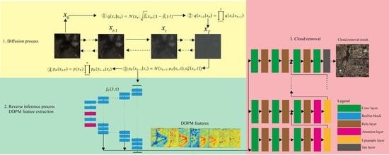
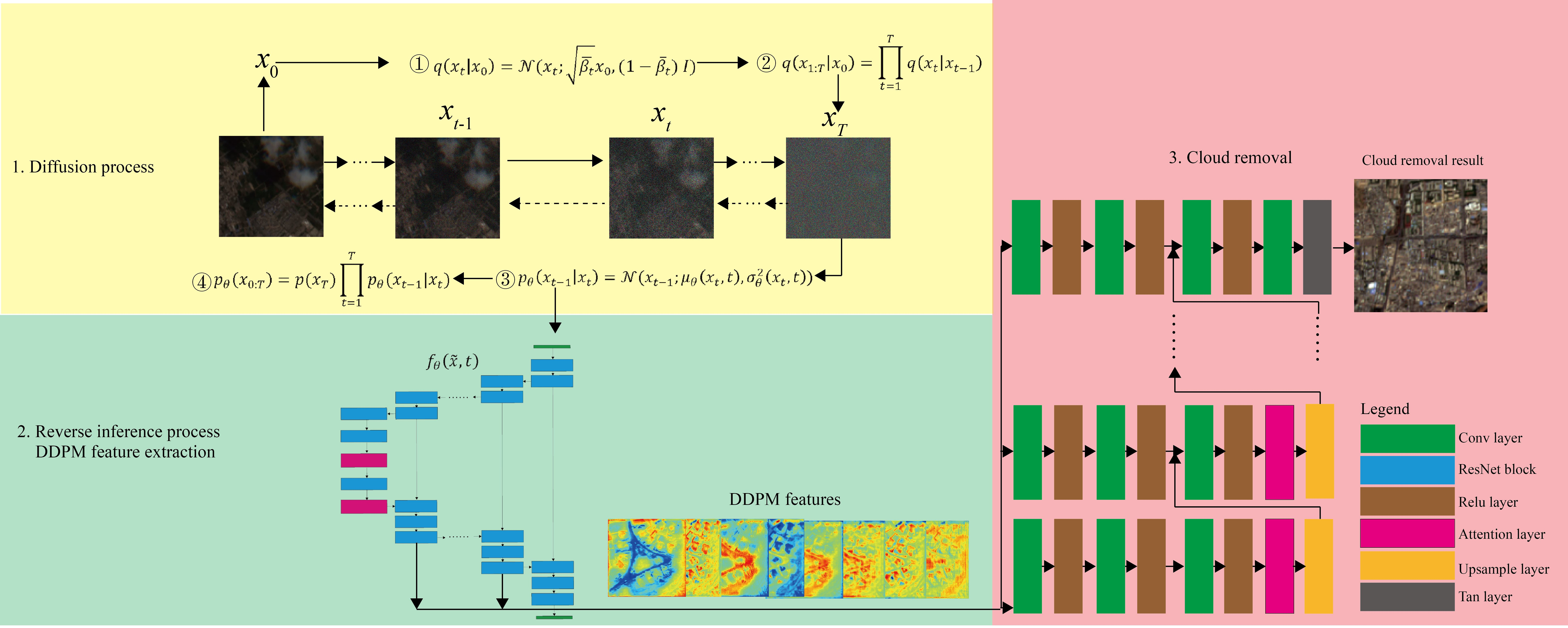
2. DDPM-CR Architecture for Cloud Removal

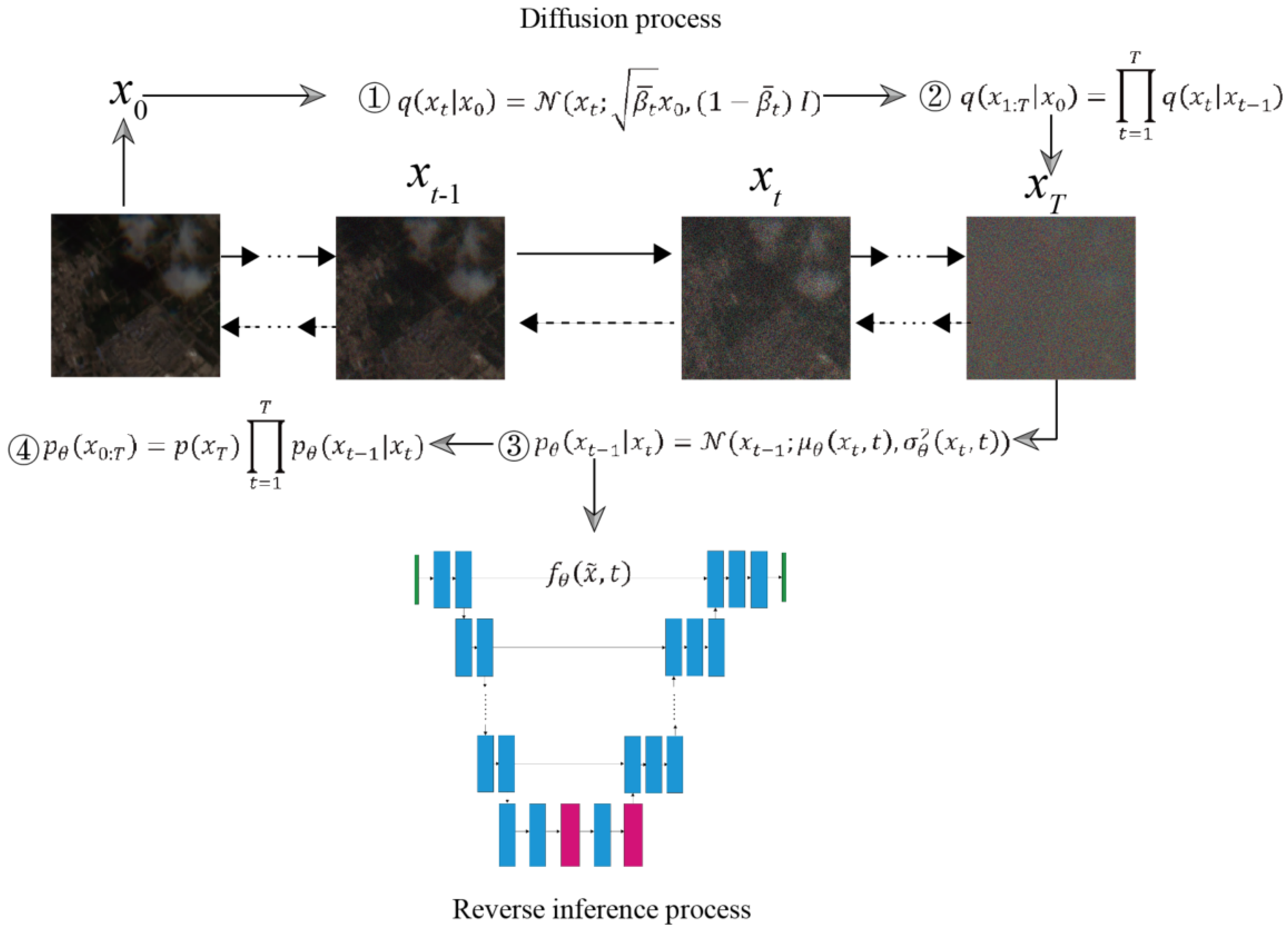
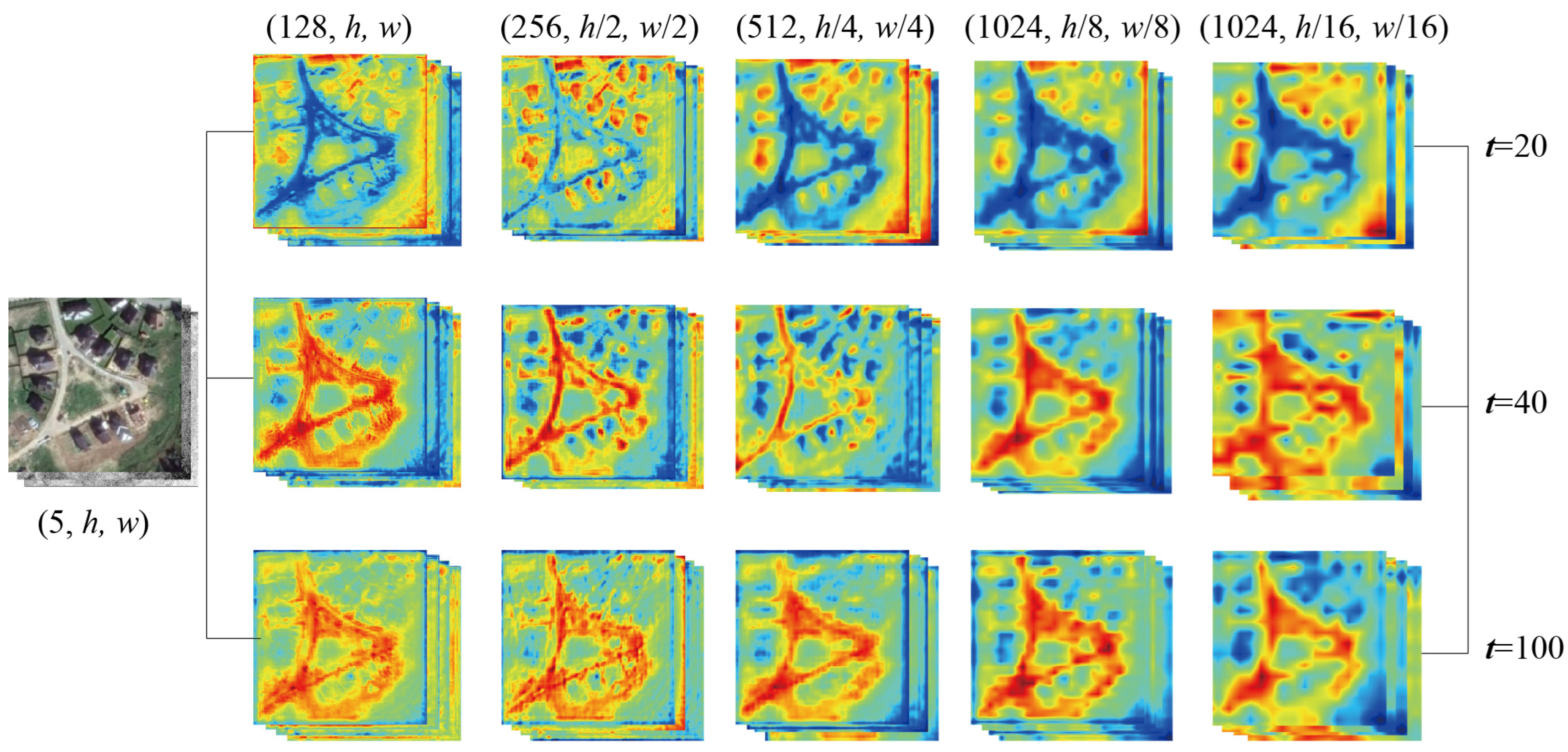
2.1. DDPM Features on Cloud Removal

The DDPM-CR methodology consists of two main components: the DDPM network and the proposed cloud removal head. The DDPM network serves to extract deep features at multiple levels, which are then fed as input to the cloud removal head. By utilizing the abundant DDPM features, the cloud removal head is able to retrieve missing information in cloud-covered images. DDPM, similar to GAN and VAE models, is a type of generative model [37], and well-trained models can generate realistic remote sensing images. Given the success of DDPM in various computer vision applications, as demonstrated in the introduction, it has the potential to be effectively applied to the cloud removal task. The DDPM network comprises two procedures, namely, the forward procedure and the reverse procedure, as depicted in Figure 1.

The DDPM forward procedure involves a Markovian process that adds Gaussian noise to remote sensing images. In the context of the cloud removal task, the cloud-contaminated image serves as x₀ and provides the initial image distribution. To ensure adequate extraction of features for the retrieval of information from cloud-contaminated images, the DDPM network employs five input bands, including three multispectral bands (red, green, and blue) and two SAR bands (VV and VH). Using the reparameterization technique depicted in Figure 1 as ①, noise-added x_t can be obtained for any time t∈(0, T) based on given hyperparameters. Here, ${\beta }_t$ controls the noise variance and $\stackrel{-}{{\beta }_t}=\prod _{i=1}^T{\beta }_i$, which are distributed on the interval from 0–1. After T iterations, as illustrated in ②, noise-added results that obey an isotropic Gaussian distribution are generated.

The reverse inference process is also a Markov chain that aims to reconstruct original images from noise-added results after T iterations, as illustrated in ③ and ④ of the above figure. This denoising procedure requires a deep network $f_{\theta }$ to model the parameters during the reverse inference. The parameters ${\mu }_{\theta }\left(x_t,t\right)$ and ${\sigma }_{\theta }^2\left(x_t,t\right)$ in ③ are the mean and variance acquired through network training. To this end, a U-Net-based [38] network is modified for reverse inference, as shown in Figure 2.

The main architecture for reverse inference is based on the widely-used U-Net network, as shown in the figure above. To meet the requirement of image recovery from noise and provide precise deep features for the subsequent cloud removal procedure, the main modified part is the ResNet block. A noise affine layer is designed to linearly add noise to image features. Additionally, a swish layer is used, as it has been shown to outperform the ReLU layer in deeper architectures [39]. To concentrate the network on deep features at different dimensions as well as various salient image regions, the high efficiency and robustness of spatial and channel attention mechanisms are introduced without obvious computational cost increasing [40]. To avoid affecting the inference performance, the attention layers are set in the bottleneck of the architecture. Finally, the original concatenated image can be reconstructed, and its objective function can be defined in a simplified form according to the works proposed by [37]:

$${𝔼}_{x_0,ϵ}{‖f_{\theta }\left(\tilde{x},t\right)-ϵ‖}_2^2,ϵ~\mathcal{N}(0,I),$$

(1)

where $f_{\theta }$ represents the above denoising model; $\tilde{x}$ is the noise-added image after the forward procedure.

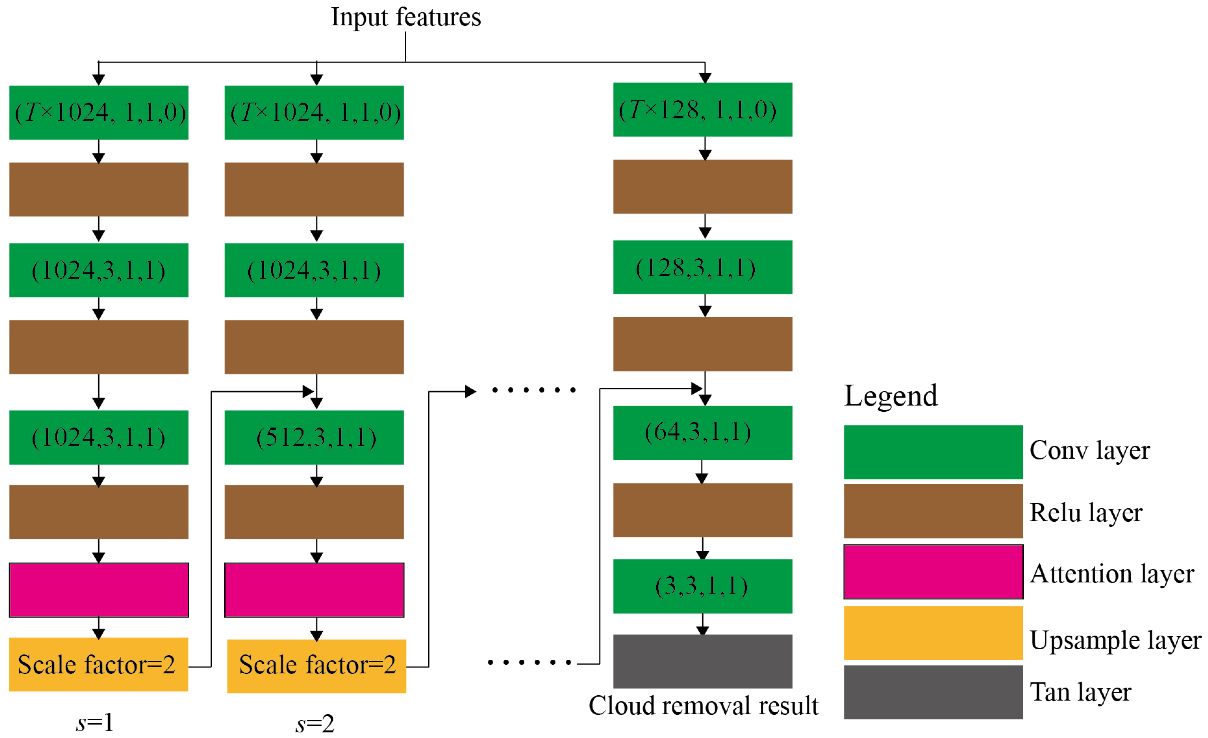
2.2. Cloud Removal Head

In this paper, we did not employ the DDPM reverse inference workflow to directly remove clouds, as retrieving missing spectral information for remote sensing images requires a more sophisticated architecture. Therefore, utilizing a well-trained DDPM network, we extracted diverse deep features to provide abundant information, which enabled us to achieve better cloud removal results via the subsequent cloud removal head. The extracted DDPM features are illustrated in Figure 3.

The figure above depicts the deep features extracted from the pretrained DDPM network. The figure is divided into 3 rows and 5 columns, with each row representing different noise levels added to input images, and each column presenting deep features at various scales. These noise levels were selected through trial and error to enhance the network’s robustness towards diverse imaging conditions. The extracted features at different scales, such as (h, w), (h/2, w/2), (h/4, w/4), (h/8, w/8), and (h/16, w/16), represent different characteristics of the image, from shallow edge and texture to global abstract representations. Both the large-scale and small-scale features can be well described. The multiscale feature representations generated by combining these features better capture the patterns in remote sensing images. Based on these deep features, we propose a cloud removal head to perform the cloud removal task, as shown in Figure 4.

The figure above depicts the cloud removal inference procedure, where deep features extracted from the DDPM network with different noise levels are used as inputs to provide effective information on the ground objects’ description at various scales. The network is composed of several blocks, with the number of blocks corresponding to the number of extracted DDPM features. Each block consists of convolutional layers, ReLU layers, attention layers (the same as the DDPM network), and upsampling layers used to recover the original size of the output image step by step. At the top of the network, the tanh layer compresses the output values to (−1, 1) to match the range of normalized input images. Additionally, at each step, the network integrates all DDPM features with the processed features to retain refined image details and then passes them to attention layers to focus on recovering missing information in cloud-contaminated regions.

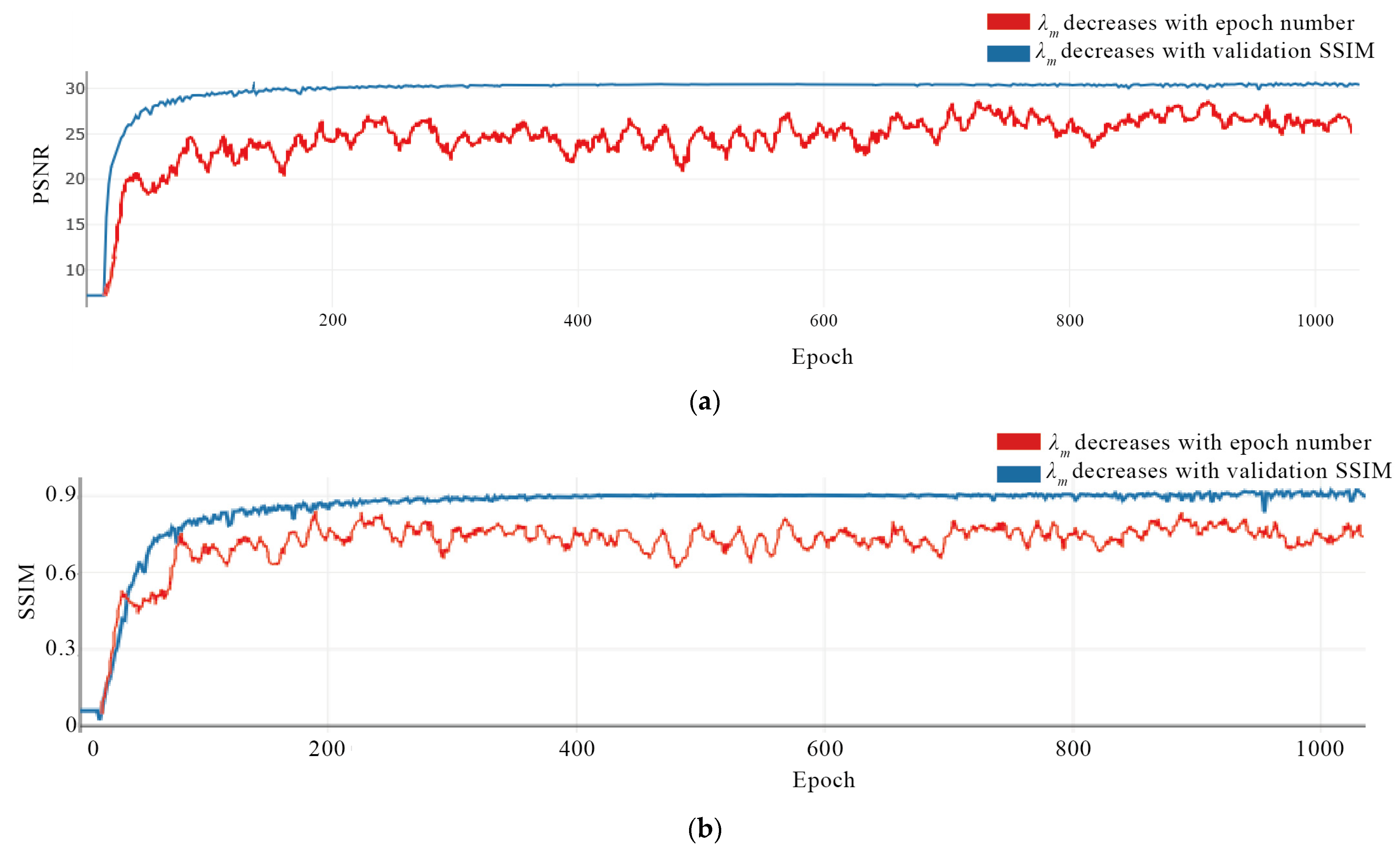
2.3. Cloud-Oriented Loss

The loss function used for training the DDPM network is described in Equation (1). However, the cloud removal head is the primary component responsible for removing clouds, and it functions similarly to image inpainting. Typically, Mean Absolute Error (MAE) loss is commonly employed in image inpainting networks. However, the cloud-contaminated pixels in remote sensing images have a high dynamic range and significant deviation. As a result, a single MAE loss function is inadequate to address this issue. To overcome this challenge, a cloud-oriented loss is proposed in this paper that incorporates three sub-loss functions, as follows:

$${\mathcal{L}}_{COL}={{\lambda }_a\ast \mathcal{L}}_{mMAE}+{\lambda }_b\ast {\mathcal{L}}_{percep}+{\lambda }_c\ast {\mathcal{L}}_{attention}.$$

(2)

The cloud-oriented loss, denoted as ${\mathcal{L}}_{COL}$, is a combination of three subloss functions, namely, the modified MAE loss (${\mathcal{L}}_{mMAE}$), perceptual loss (${\mathcal{L}}_{percep}$), and attention loss (${\mathcal{L}}_{attention}$), weighted by ${\lambda }_a$, ${\lambda }_b$, and ${\lambda }_c$, respectively. The modified MAE loss accounts for both clouds and cloud shadows and its definition depends on the validation accuracy metrics used, as depicted in the following equation:

$${\mathcal{L}}_{mMAE}={\lambda }_M\ast {‖G-P‖}_1+\left(1-{\lambda }_M\right)\ast {‖M⨀\left(G-P\right)‖}_1,$$

(3)

where G and P represent the target cloudless image patch and the cloud removal result obtained by the cloud removal head, respectively. The L1 loss, also known as the MAE loss, is denoted by ${‖\ast ‖}_1$ and the Hadamard product is represented by $⨀$. The cloud and cloud shadow mask, M, is obtained from the cloud detection method proposed by Zhai et al. [41]. The weights of the cloud-free and cloud-contaminated regions are denoted by ${\lambda }_M$, which change during the training procedure based on the validation accuracy metrics. When the accuracy is low, ${\lambda }_M$ is set to a high value to enable the network to learn the overall characteristics of remote sensing images. As the network training progresses and the accuracy improves, ${\lambda }_M$ is gradually decreased to focus the network on recovering missing information.

The modified MAE loss function aims to reconstruct the color and texture information of the image patches, while during the training process, high-frequency information may be lost, leading to oversmoothed results. To address this issue, the cloud-oriented loss includes a perceptual loss term (${\mathcal{L}}_{percep}$). This term leverages pretrained CNN networks to measure the difference between the generated image patch and its corresponding cloudless patch, enhancing the details of the cloud removal results [42]. Additionally, attention loss is also incorporated into the cloud-oriented loss, as defined by the following equation.

$${\mathcal{L}}_{attention}={‖A-M‖}_2^2$$

(4)

The attention loss function plays a crucial role in the cloud-oriented loss by integrating the features obtained from each attention layer in Figure 4 and generating a spatial attention matrix, which enhances the image regions of clouds and cloud masks at various scales as high salient values, improving the overall performance of the cloud removal task. ${‖\ast ‖}_2^2$ denotes the L2 loss function, which is used to control the network to focus on the cloud removal task. After extensive experimentation, ${\lambda }_a$, ${\lambda }_b$, and ${\lambda }_c$ are chosen as 0.8, 0.15, and 0.05, respectively, to balance different remote sensing image representations.

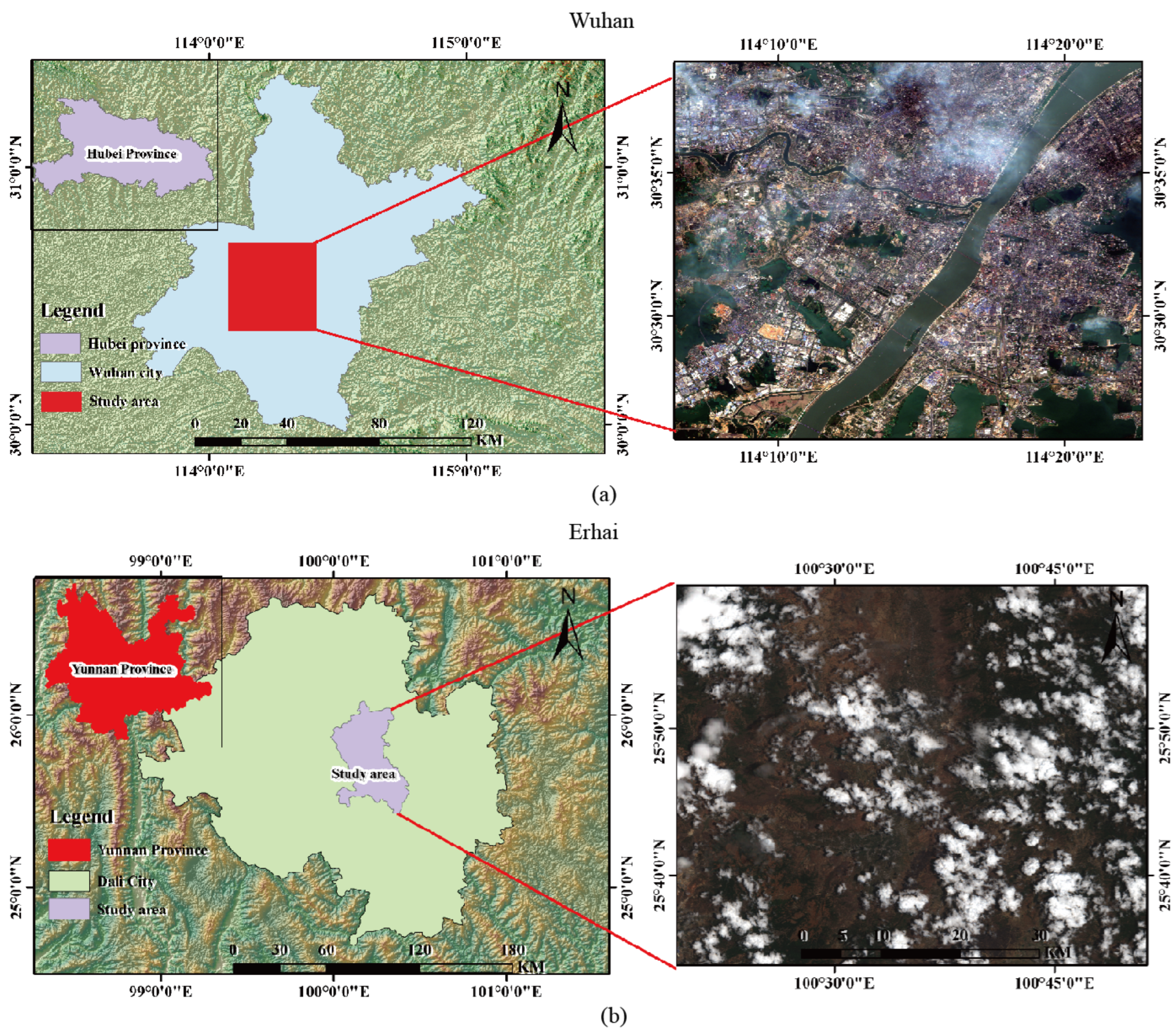
2.4. Experimental Data and Training Details

To train the DDPM-CR network, a large number of image patches are required, particularly for complex remote sensing image representations. In this study, we utilize Sentinel-1 and Sentinel-2 images for cloud removal tasks due to their spatial–temporal resolution and accessibility [43,44]. The Sentinel-2 multispectral data capture spectral signals ranging from 443 nm to 2190 nm with 13 bands at different spatial resolutions. The spatial resolution of visible and NIR bands is 10 m, while other bands have spatial resolutions of 20 m and 60 m. On the other hand, the Sentinel-1 satellite can acquire ground information on all weather conditions with several imaging modes. The most widely used mode is the interferometric wide swath (IW), which captures single-polarized VV and dual-polarized VH image data. To train the DDPM-CR network effectively under various cloud conditions, we introduce an open-source dataset named SEN12MS-CR [45], which contains 175 globally distributed regions in 4 seasons throughout 2018. The dataset comprises 122,218 image triplets (SAR, cloudy, and target cloudless images) with a size of 256 × 256. In this paper, we define thick cloud regions as image regions where over 60% of the spectral signal is completely obstructed by clouds, and vice versa. We use the partition criteria in

Table 1. The number of training, validation, and test samples of the SEN12MS-CR dataset. The partition ratio is 6:2:2.

Dataset	Train Samples	Validation Samples	Test Samples
SEN12MS-CR	73,331	24,444	24,443

for network training, validation, and testing.

In this work, preprocessing of the multimodal data sources, Sentinel-2 multispectral images and Sentinel-1 SAR images, was performed to address their significant differences in value ranges and eliminate the impact of anomalous and background pixels on the results. Anomalous value filtering and min–max normalization were utilized for the data preprocessing. The anomalous value filtering procedure eliminated the effect of outlier pixel values on normalization. The minimum and maximum values of the multispectral and SAR images were calculated by iterating through the entire dataset. After preprocessing, the value range of each image data item was transformed to [−1, 1] to avoid the influence of different value dimensions. Additionally, random image cropping was employed during network training to randomly clip the original image patches into smaller-sized subsets. The generation of image patches at different locations in each iteration added robustness to the network. Furthermore, smaller-sized image patches resulted in fewer DDPM feature parameters, reducing the burden on GPU memory.

The training procedure for the DDPM and cloud removal head network is a two-step process. To ensure uniformity, the row and column sizes for all training image patches are randomly cropped to 128. For the DDPM network, a learning rate of 1 × 10⁻⁴ and an Adam optimizer with a cosine warmup schedule are used. The weights are initialized with a Kaiming distribution to maintain heterogeneity and stability of weight parameters. In contrast, the cloud removal head network applies a normal distribution with μ = 0 and δ2 = 0.02 to initialize the weights. Similarly, the Adam optimizer is also used with β1 = 0.5 and β2 = 0.999, and the initial learning rate is 2 × 10⁻⁴ for the first 50 epochs, followed by a multistep decay method with a decay rate of 0.92 for better convergence. The training process for both networks runs for a total of 200 epochs with a batch size of 1 due to GPU memory limitations.

The implementation platform is a workstation equipped with an Intel Core i9-10900k CPU @ 3.70 GHz, 32 GB of DDR4 2133 MHz RAM, and an NVIDIA GeForce RTX 3060 with 12 GB RAM. The operating system is Ubuntu 18.04. All networks were implemented with PyTorch 1.10.0 using Python 3.6. Please refer to the Supplementary Materials section for the implementation of DDPM-CR.

To quantitively evaluate the performance of the cloud removal results, four metrics are used for analysis, MAE, RMSE, PSNR, and SSIM, and the definitions are listed as follows.

(1)

Mean absolute error (MAE)

$$\mathrm{M}\mathrm{A}\mathrm{E}=\frac{1}{H\times W}{\sum }_{i=1}^H{\sum }_{j=1}^W\left|P(i,j)-G(i,j)\right|,$$

(5)

where MAE is defined as the deviation of the inferred result and the target image. H and W depict height and width, respectively. (i, j) represents the pixel location of the image patch, and P (i, j) and G (i, j) are pixel values in the inferred and target images, respectively.

(2)

Root-mean-square error (RMSE)

$$\mathrm{R}\mathrm{M}\mathrm{S}\mathrm{E}=\sqrt{\frac{1}{H\times W}{\sum }_{i=1}^H{\sum }_{j=1}^W\left(P\right(i,j)-G(i,j){)}^2},$$

(6)

where RMSE is also a widely used pixel-level metric for similarity calculation between inferred and target images with the square root of mean square residual error.

(3)

Peak signal-to-noise ratio (PSNR)

$$\mathrm{P}\mathrm{S}\mathrm{N}\mathrm{R}=10{\mathit{log}}_{10}(\frac{(2^n-1{)}^2}{\mathrm{M}\mathrm{S}\mathrm{E}}),$$

(7)

$$\mathrm{M}\mathrm{S}\mathrm{E}=\frac{1}{H\times W}{\sum }_{i=1}^H{\sum }_{j=1}^W\left(P\right(i,j)-G(i,j){)}^2.$$

(8)

PSNR is an objective assessment metric for image evaluation, and it reflects the image reconstruction quality. Within the equation definition, MSE is defined as the mean square error between inferred and target images. Generally, a PSNR value lower than 20 indicates poor reconstruction quality, and a PSNR value over 30 shows excellent reconstruction performance. PSNR is often used with the SSIM metric.

(4)

Structural similarity (SSIM)

The SSIM metric is a common metric used to measure the similarity of inferred and target images. It applies intensity (s), brightness (l), and contrast (c), as defined below.

$$\left\{\begin{array}{c}l(P,G)=\frac{2{\mu }_P{\mu }_G+C_1}{{\mu }_P^2+{\mu }_G^2+C_1}\\ c(P,G)=\frac{2{\sigma }_P{\sigma }_G+C_2}{{\sigma }_P^2+{\sigma }_G^2+C_2}\\ s(P,G)=\frac{{\sigma }_{PG}+C_3}{{\sigma }_P{\sigma }_G+C_3}\hspace{0.33em}\hspace{0.33em}\hspace{0.33em}\end{array}\right.,$$

(9)

where μ_P, μ_G, σ_P, σ_G, and σ_PG are the mean, standard deviation, and covariance of the inferred and target images, respectively. C₁, C₂, and C₃ are constants to avoid INF results, C₁ = (K₁ ∗ L)², C₂ = (K₂ ∗ L)², and C₃ = C₂/2 with K₁ = 0.01 and K₂ = 0.03. L is determined according to grayscale for 16-bit Sentinel images, L = 65,535. To increase the execution efficiency, a Gaussian function is used to calculate the mean, standard deviation, and covariance. Therefore, the final SSIM definition is listed as follows.

$$\mathrm{S}\mathrm{S}\mathrm{I}\mathrm{M}=\left[l\right(P,G\left){]}^{\alpha }\right[c(P,G){]}^{\beta }\left[s\right(P,G){]}^{\gamma },$$

(10)

where α, β, and γ are weights to define the importance of l, c, and s, respectively, with α = β = γ = 1.

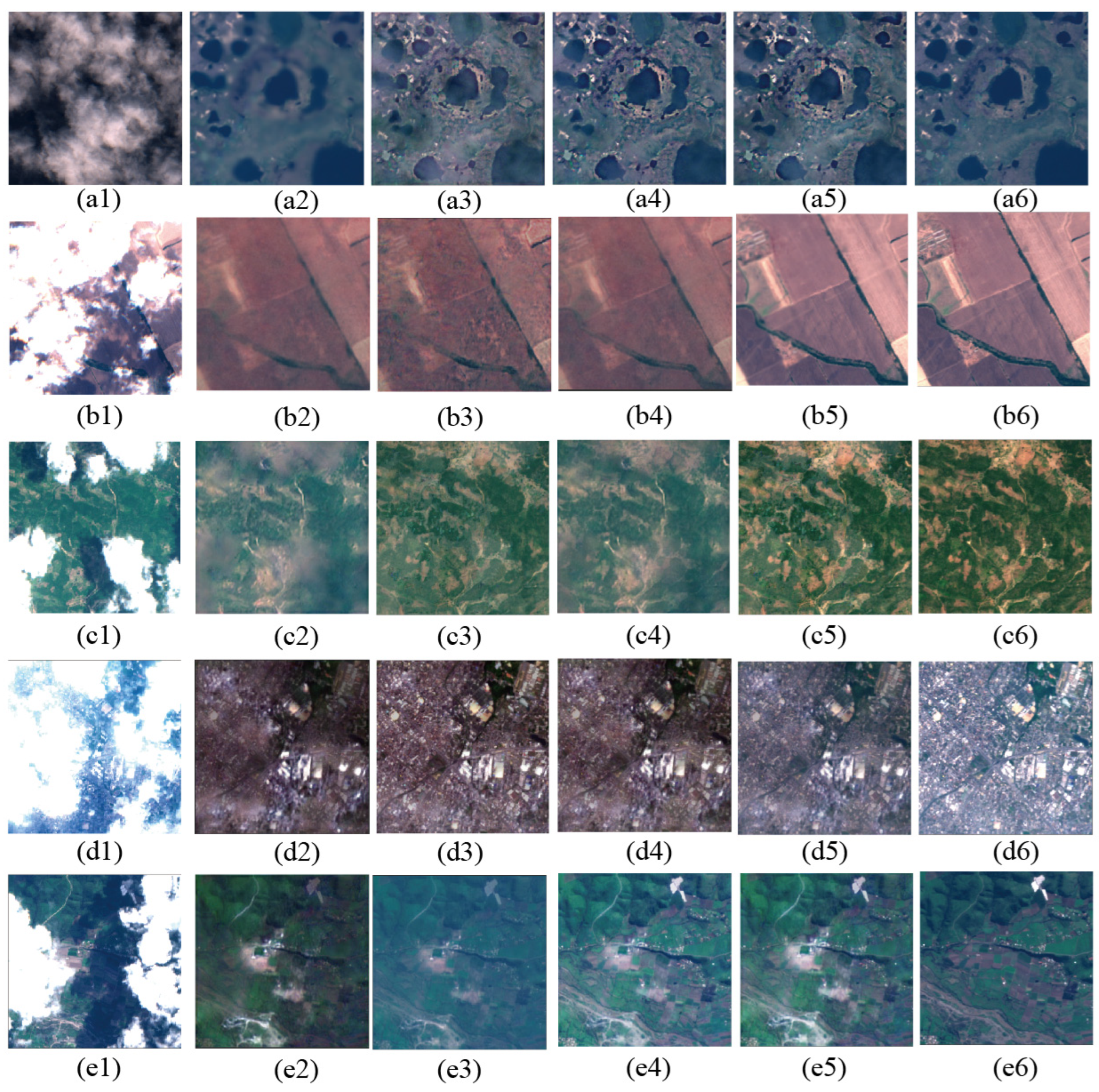
3. Experiments and Results

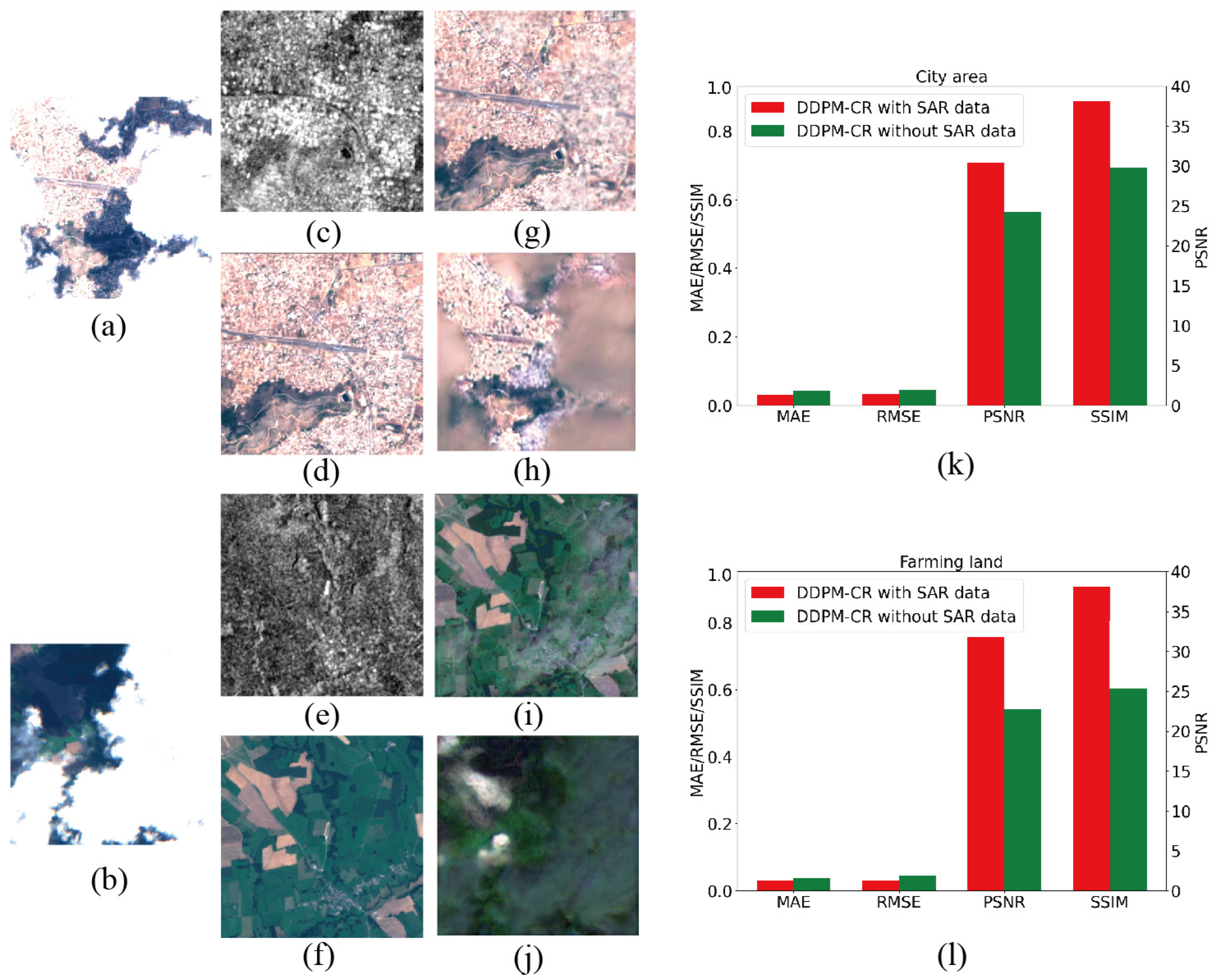
3.1. Ablation Study on SAR-Multispectral Multimodal Input Data

Most cloud removal methods use only optical images as data sources. However, under this condition, some spectral information is needed to penetrate clouds, making cloud removal challenging. Thick clouds obstruct ground object spectral information recorded by satellite image sensors, and these methods rely solely on the neighbor image representations of clouds to recover the missing information. By incorporating SAR images as complementary data, the missing information in thick cloud-covered regions is more likely to be recovered. To validate the impact of multimodal input data on cloud removal, an identical DDPM-CR network without SAR images is trained. The results are presented in Figure 5.

The effectiveness of SAR data is demonstrated in the above figure, which includes examples of city areas and farming land. City areas have complex textures, making it difficult to retrieve missing information, while farming land is more homogeneous in image representation but is affected by the seasonal aspect of plants. Both areas are covered with thick clouds and cloud shadows, and information on most image parts is missing except for the upper-left corner. The DDPM-CR network, with auxiliary SAR data, outperforms the network trained without SAR data in both areas. In the city area, (g) shows that missing information in cloud-covered regions is well recovered, whereas without auxiliary information, missing information cannot be well reconstructed, and the reconstruction parts have traces of clouds, as shown in (h). For farming land, the network without auxiliary data can only infer missing information using neighboring pixels, leading to failure in retrieving both cloud-covered and cloud-free regions, as shown in (j). Evaluation metrics of the cloud removal results are shown in (k) and (l). To reduce the difference in measurement units, MAE, RMSE, and SSIM metrics share a common axis, and PSNR uses an individual axis. In addition, MAE and RMSE are in small values, and the bars are much shorter than those of SSIM. From the two subfigures, SAR data contribute to better performance, with each accuracy metric higher than that of the non-SAR data network. The MAE and RMSE metrics are relatively close for specific regions, and significant improvements appear in the PSNR and SSIM of the farming land region, where the inferior cloud removal result without SAR data complement enlarges the gap between the result with SAR data. To further assess the effectiveness of SAR data, an evaluation table is generated with the test dataset of SEN12MS-CR, as listed in

Table 2. The quantitative results of the DDPM-CR network with or without SAR data complementation. The metrics below are achieved by mean values of the test dataset from SEN12MS-CR. In the table, the first row denotes the DDPM-CR network trained with SAR data as a complement, and the second row refers to the network trained without SAR complementation.

Training Strategy	MAE	RMSE	PSNR	SSIM
With SAR as a complement	0.0301	0.0327	29.7334	0.8943
Without SAR as a complement	0.0394	0.0432	26.3421	0.7334

.

Table 2 demonstrates that the DDPM-CR network trained with and without SAR data yields different results. Figure 5 also shows that the DDPM-CR network trained with SAR data outperforms the network without SAR data, as evidenced by the improved accuracy metrics. By incorporating SAR data as auxiliary data, the MAE and RMSE metrics decrease by 30.9% and 32.1%, respectively, while the PSNR and SSIM metrics increase by 12.8% and 21.9%, respectively. The SAR data are crucial in providing additional information to assist the network in retrieving the missing information. The DDPM-CR network cannot create cloud removal results without a basis, and the clouds and cloud shadows have too many types to learn their image mapping on actual ground objects, which could lead to the collapse of cloud removal results, such as the farming land result in Figure 5. By fully utilizing the spatial information of SAR images that are unaffected by clouds and cloud shadows, the network can make use of more auxiliary information to retrieve missing information. The DDPM architecture integrates the advantages of both SAR and multispectral images effectively, and the cloud removal head assembles these deep features at various noise levels in a cascading manner to attain fine cloud removal results.

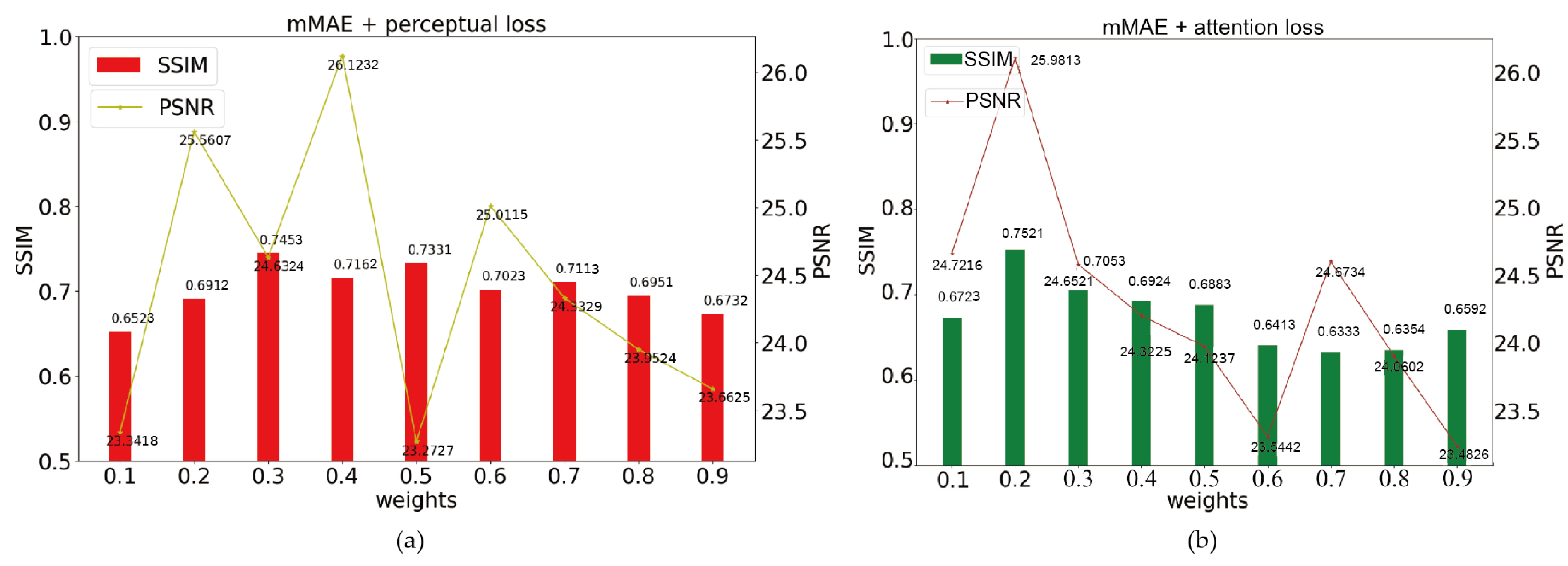
3.2. The Evaluation of Loss Functions on Cloud Removal

The performance of a deep network is greatly influenced by its loss function. In this study, we propose a cloud-oriented loss function to guide the training of the network. This loss function consists of a modified mean absolute error (MAE) loss, a perceptual loss, and an attention loss, all tailored for cloud removal. To evaluate the effectiveness of the cloud-oriented loss function, we compare the prediction results of the DDPM-CR network trained with different loss functions, namely, modified MAE loss only, modified MAE with perceptual loss, modified MAE with attention loss, and cloud-oriented loss. Before training, we determine the weights of the modified MAE loss in each comparison loss function to achieve optimal accuracy, with SSIM and PSNR as evaluation metrics, as shown in Figure 6.

The figure above illustrates the impact of different weight configurations of loss functions on the SSIM and PSNR metrics of DDPM-CR. It is evident that different weight values lead to significant differences in the results, with both SSIM and PSNR showing a rise and fall trend as the weights increase from (a) to (b). The peak values indicate the local optimal accuracy, implying that alternative weight values can be selected. In (a), the mMAE + perceptual loss function is depicted, and the peak SSIM and PSNR values occur at weight values of 0.3 and 0.4, respectively. However, the weight value of 0.3 results in more artifacts in the cloud removal results, thus, 0.4 is selected as the weight of mMAE, and the weight of the perceptual loss is set to 0.6. In (b), the mMAE + attention loss function is shown, and the peak values of SSIM and PSNR correspond to a weight value of 0.2. Therefore, the weight of mMAE is set to 0.2, and that of the attention loss is 0.8. The DDPM-CR network is trained with the chosen weights of the two loss functions, and a visual comparison of the cloud removal results is presented in Figure 7.

The subfigures (a1)–(e1) in Figure 7 show image patches heavily covered with thick clouds, which allows for evaluating the influence of the loss functions on the network performance. Subfigures (a2)–(e2) depict the results of the DDPM-CR network trained with only mMAE loss, which considers image representations of cloud-free and cloud-contaminated regions. Although missing information is recovered in all image scenes, the results lack detail, and some artifact pixels are visible, especially in regions with regular textures, such as the city region (d2).

As for the combined loss functions, subfigures (a3)–(e3) from the DDPM-CR network trained with mMAE + perceptual loss show better visual effects, with more delicate spatial information. This is due to the perceptual loss function, which greatly improves the high-frequency information in the reconstruction results with the aid of extracted features from other assistant networks, as evident in the result of (d3). However, in some homogeneous regions, such as farming lands, excessive phenomena exist. Subfigures (a4)–(e4) show the results of mMAE + attention loss, which performs better than the results of mMAE loss alone and is similar to those of mMAE + perceptual loss. Attention loss applies features from attention blocks to construct attention masks, and together with cloud masks, the training procedure is under good guidance, leading to a good recovery of missing cloud-covered and cloud-free region information. Different from the mMAE loss function mechanism, attention loss urges the network to focus more on the information retrieval of cloud-covered regions. The reconstruction results have a better natural visual representation compared with the other two loss functions, reflecting the complementarity of mMAE and attention loss.

Subfigures (a5)–(e5) show the results of the cloud-oriented loss function, which integrates the advantages of the other three loss functions by considering the spectral information of both cloud-covered and cloud-free regions, as well as their detailed information. Its results are more consistent with the target cloudless image patches in subfigures (a6)–(e6).

Table 3. Quantitative evaluation of the loss functions on the performance of the DDPM-CR network. The metrics below are achieved by mean values of the test dataset from SEN12MS-CR. The first row lists the results of the DDPM-CR network trained with only the mMAE loss function. The second row lists the accuracy metrics with the mMAE + perceptual loss function. The third row lists the results of the mMAE + attention loss function. The fourth row lists the results of the cloud-oriented loss function.

Loss Function	MAE	RMSE	PSNR	SSIM
Sole mMAE loss	0.0524	0.0672	22.3123	0.6073
mMAE + perceptual loss	0.0396	0.0423	25.8741	0.7371
mMAE + attention loss	0.0458	0.0312	24.9611	0.7282
Cloud-oriented loss	0.0301	0.0327	29.7334	0.8943

is also presented below to illustrate the superiority of the cloud-oriented loss function compared with other loss functions.

As listed in the above table, since the same test dataset of SEN12MS-CR is used, the metric values of cloud-oriented loss are the same as those in Table 2. Specifically, mMAE loss alone achieves the worst result among the loss functions, while cloud-oriented loss achieves the best result for MAE. For RMSE, mMAE + attention loss achieves the best value, and cloud-oriented loss comes in second place, indicating that attention loss is a stable improvement for the cloud removal task. PSNR and SSIM provide a qualitative assessment of reconstructed images, and cloud-oriented loss significantly outperforms the other loss functions. These results demonstrate that cloud-oriented loss effectively integrates the advantages of the other loss functions and yields more comprehensive results. Together with the analysis in Section 3.1 and Section 3.2, the choice of appropriate loss functions, in addition to elaborately designed networks and auxiliary data such as SAR images, is crucial in improving the validation accuracy of the DDPM-CR network. Finally, the complete DDPM-CR network is compared with some baseline models.

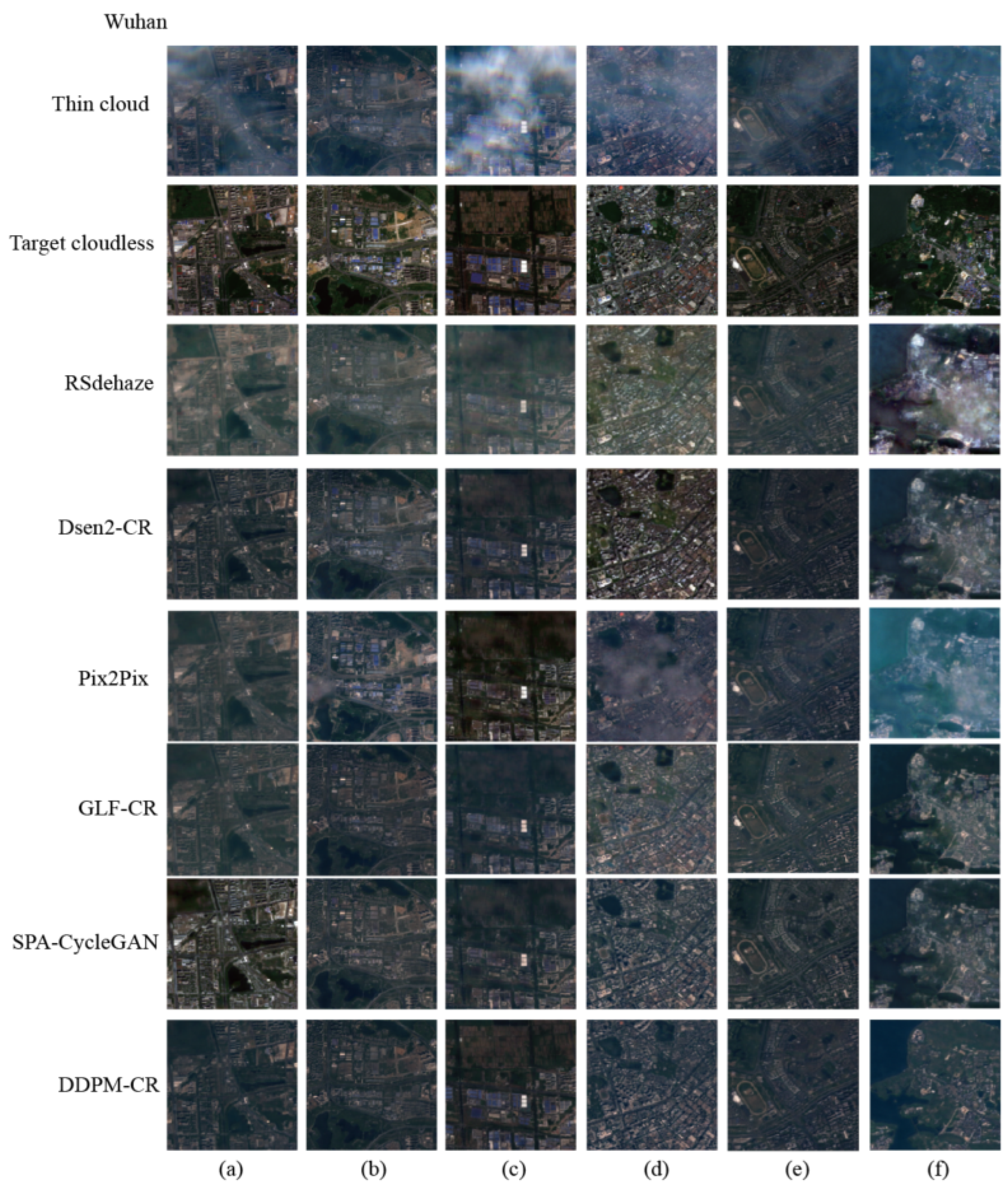
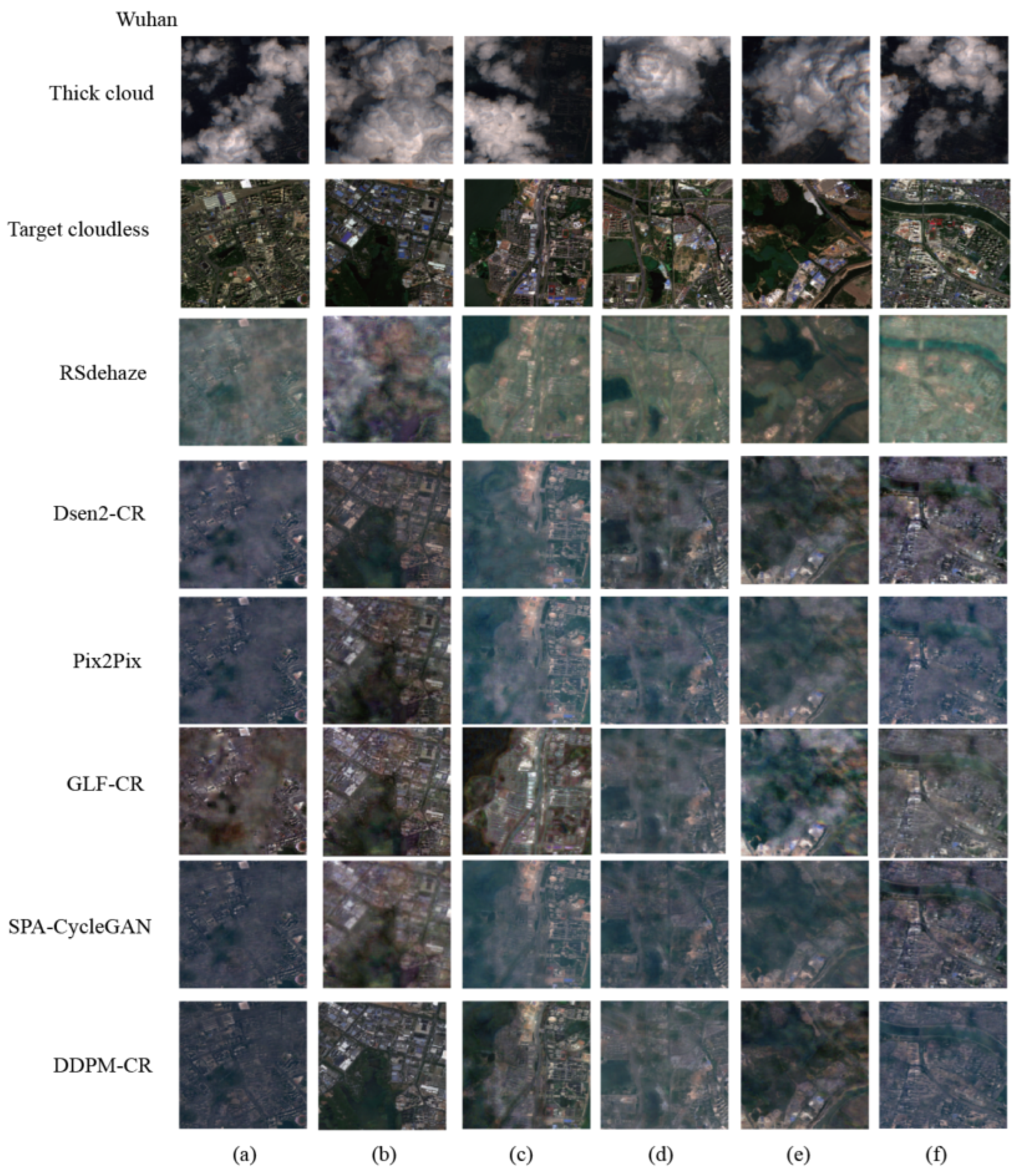
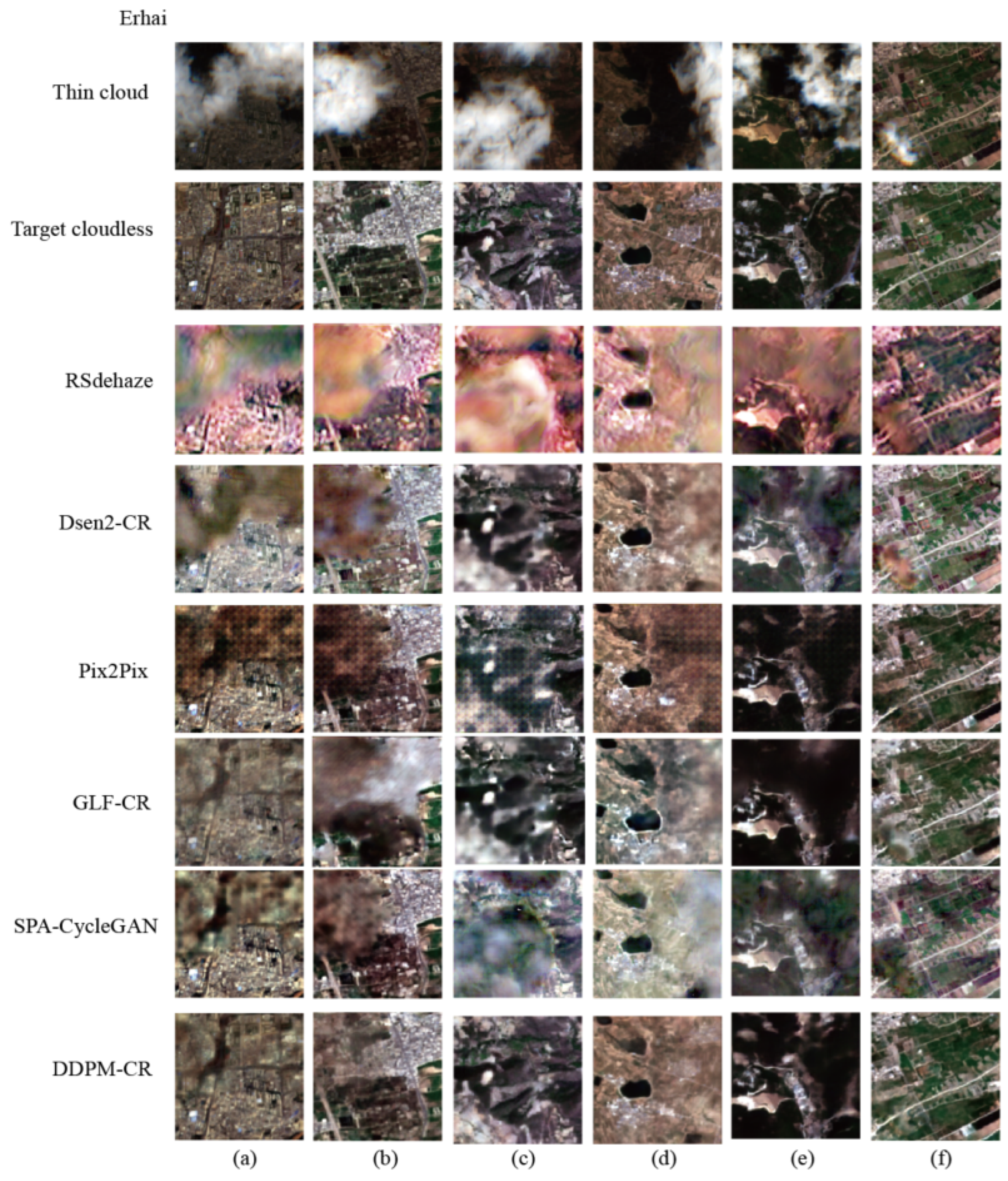
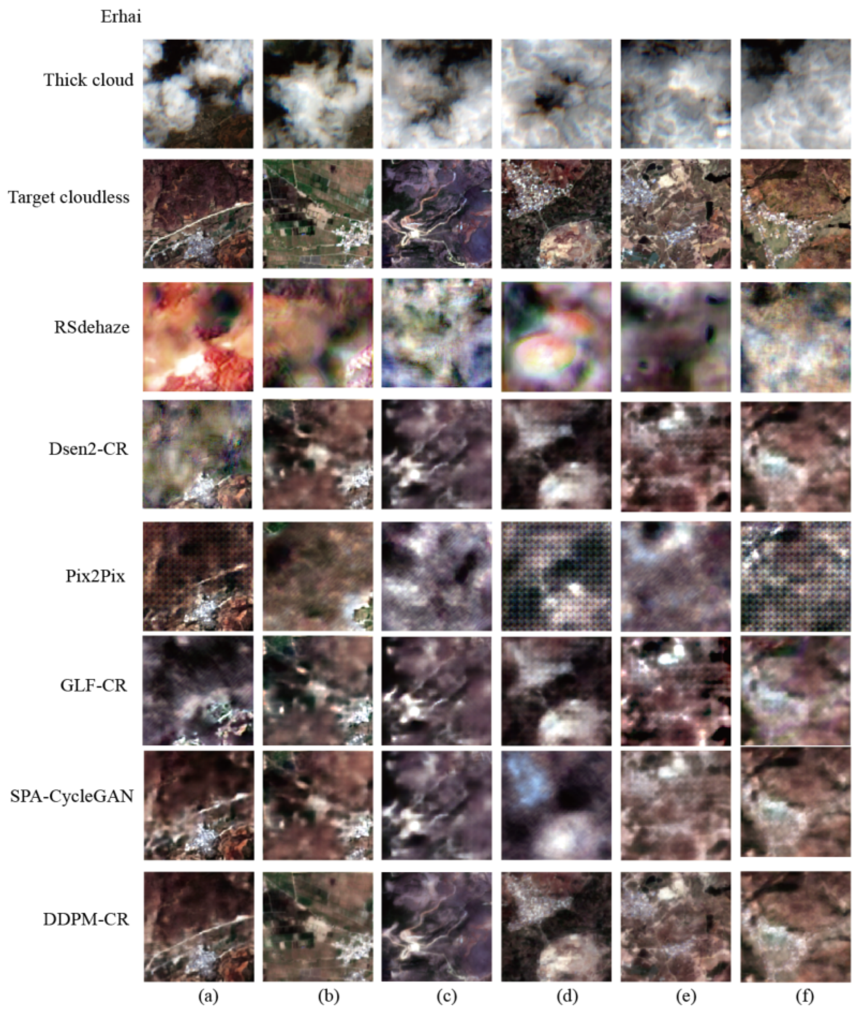
3.3. Comparative Experiments with Baseline Models

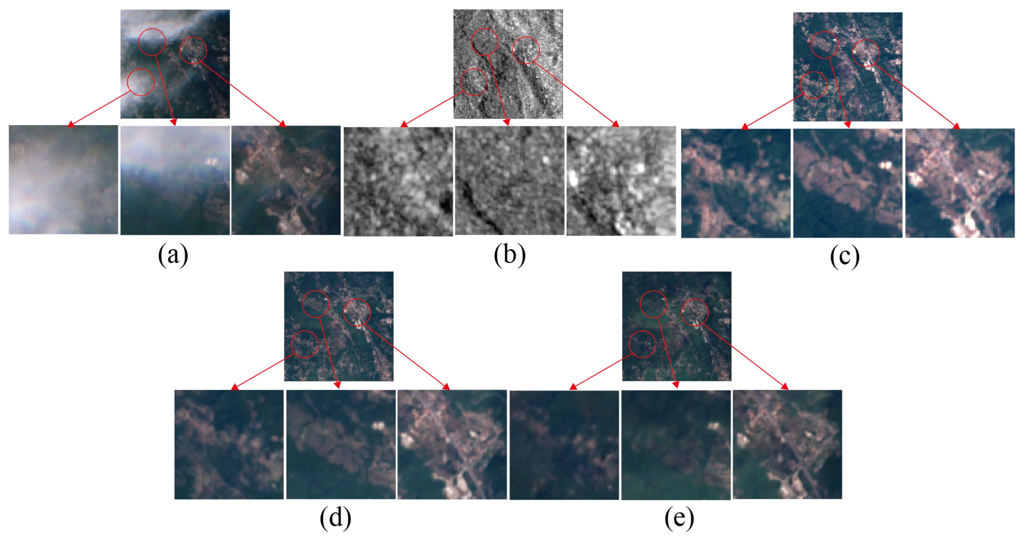
The above analyses are crucial in evaluating the effectiveness of the DDPM-CR network using the SEN12MS-CR dataset. However, to ensure the practical applicability of the network, it is essential to evaluate its performance on additional study areas. In this study, we selected two areas, Wuhan and Erhai, as shown in Figure 8, for further evaluation of the DDPM-CR network.

Erhai is located in Dali Bai Autonomous Prefecture, Yunnan Province, China. It is the second-largest freshwater lake in Yunnan [46]. Erhai is long and narrow in shape, and its bank side is steep. The annual water temperature ranges from 12–21 °C. Due to its unique geographical characteristics, Erhai is frequently covered by clouds that severely affect crop-monitoring-related tasks. Wuhan is in the middle and lower reaches of the Yangtze River, and it is a central city of transportation hubs, industrial centers, and science and education centers. Rapid city expansion requires high-quality remote sensing images to assist in regulation. However, the Yangtze River and abundant rainfall cause this area to be regularly covered with a high percentage of cloud coverage. For image data, SAR, cloudy and cloudless images should be collected on adjacent dates to ensure that target cloudless images are available. For the Erhai area, SAR and cloudy images were acquired on 13 August 2020, cloudless images were acquired on 27 August 2020, and those images of Wuhan were acquired on 7 August 2022 and 17 August 2022. The images of the two study areas were split into 128 × 128 size patches with thin cloud and thick cloud regions separately to make a dataset for evaluation of the comparison methods.

To evaluate the effectiveness of the DDPM-CR network, we compare it against a traditional method, RSdehaze [47], and four other deep learning networks: DSen2-CR [24], pix2pix [48], GLF-CR [23], and SPA-CycleGAN [30]. The RSdehaze method is used to highlight the importance of auxiliary SAR images in cloud removal. GLF-CR uses a two-stream network that differs from DDPM-CR, while the other deep learning methods are similar in many ways to DDPM-CR. DSen2-CR is a ResNet-based network that takes cloud masks into account, while pix2pix and SPA-CycleGAN are generative models like DDPM-CR. SPA-CycleGAN also incorporates an attention mechanism and corresponding attention loss. To ensure a fair comparison, all deep learning methods use SAR images as complementary data and are trained using the SEN12MS-CR dataset. The cloud removal results of the comparison methods on the two study areas are presented in Figure 9, Figure 10, Figure 11 and Figure 12.

The spectral signal can penetrate clouds to a certain extent, allowing it to be captured by satellite sensors. This phenomenon is similar to fog and can be partially corrected through radiation correction in remote sensing preprocessing. In Figure 9, the comparison methods used in Wuhan study area achieved good results, with thin clouds being completely removed. However, clouds and cloud shadows generally have a greater impact on the RSdehaze algorithm, leading to reconstruction failure in cloud-covered regions. This highlights the importance of SAR images in cloud removal tasks.

The pix2pix network also faced difficulties in synthesizing multiple information types to generate target cloudless images, which may explain its lower performance. In contrast, the DSen2-CR network achieved better visual results than the GLF-CR network, displaying more detailed building textures. In Figure 9a, SPA-CycleGAN performs well and generates results that are more consistent with the target image than DDPM-CR, while DDPM-CR achieves better results in other regions.

The first two rows in Figure 10 demonstrate that thick clouds completely obstruct the transmission of the spectral signal in Wuhan study area, resulting in denser clouds and shadows compared with thin cloud conditions. The RSdehaze method exhibits severe deterioration in the results, with color mistakes and failure to recover detailed construction information, even cloud-like artifacts, particularly in region (b). Deep-learning-based methods also produce degraded results with a blurred appearance in the recovered image information within thick cloud regions.

Specifically, Dsen2-CR and pix2pix achieve similar results with inferior visual effects, while GLF-CR outperforms other comparison methods in regions (b) and (c) with finer color and detailed information due to its two-stream architecture. The SPA-CycleGAN network demonstrates good results in regions (d) and (f), owing to the attention mechanism adopted in the architecture that plays a significant role in cloud locating and missing information reconstruction. However, overall, the DDPM-CR network outperforms other methods, as it retrieves a majority of spectral information under thick clouds and cloud shadows and produces the least vagueness in cloud removal results.

In Figure 11 of Erhai study area, the diversity of ground objects poses more challenges to the comparison methods than in Wuhan, as both natural and man-made objects are present. Additionally, cumulus clouds are widespread in the area, further hindering spectral information transmission compared with Wuhan. The denser clouds in Erhai result in more distorted cloud removal results and inconsistent colors with the target cloudless images when using RSdehaze methods. Deep learning-based methods, aided by auxiliary SAR images, can retrieve missing data from clouded areas, with good reconstruction results in cloud-free regions.

However, denser clouds and a diverse range of ground objects introduce additional complexity to the cloud removal task and all deep learning-based methods have limitations in accurately reconstructing cloud-contaminated regions. The pix2pix network exhibits poor generalization, with mosaic artifacts in cloud-contaminated regions. GLF-CR retrieves more image information on cloud regions than DSen2-CR, particularly in region (a), while DSen2-CR has limited performance in this study area. The SPA-CycleGAN and DDPM-CR networks, which share similar principles, achieve comparable results, with DDPM-CR producing finer details in regions (a) and (c).

The Figure 12 presents the results of thick cloud removal achieved by comparison methods in the Erhai study area. In the first row of the figure, it is difficult to distinguish the image representations, and thick clouds occupy most of the scene. The RSdehaze method fails to produce reasonable results, and even the DSen2-CR network shows vague representations, even if thick clouds cannot be identified. The results obtained by the pix2pix network display numerous mosaic artifacts with a blurred appearance. GLF-CR generates mosaic-like artifacts in (d) and (e). Although SPA-CycleGAN retrieves some of the missing information caused by thick cloud coverage, the results are still vague, similar to those of the GLF-CR network. In contrast, the proposed DDPM-CR network outperforms other methods in terms of cloud removal results with a better visual appearance, such as the results shown in (d). Other methods fail to reconstruct the detailed information of the town region in the scene, while the DDPM-CR network recovers this information with less distortion.

In the results of the comparison methods for various cloud thicknesses, deep learning-based methods outperform the traditional RSdehaze method in two aspects. Firstly, the RSdehaze method is designed specifically for fog and thin cloud removal applications, and its performance is severely reduced under thick clouds. Secondly, it only uses optical bands, which makes information recovery under thick clouds ineffective. Each network has its area of expertise, and the above results indicate that the pix2pix network, without modification, cannot be used directly for cloud removal tasks. The two-stream architecture of GLF-CR does not show a significant improvement compared with one-stream architectures, and it has similar performance to DSen2-CR. SPA-CycleGAN is similar to the DDPM-CR network in both architecture and loss function definition, which contributes to better cloud removal results. The proposed DDPM-CR network builds on the successful experience of previous works to improve its performance on the cloud removal task, and its inference results are less affected by cloud thickness compared with other methods.

Table 4. Evaluation of DDPM-CR and comparison methods in Wuhan and Erhai. The evaluation results are achieved under thin and thick cloud conditions to separately validate the performance of these cloud removal methods.

Model	MAE	RMSE	PSNR	SSIM
Wuhan
Thin cloud
RSdehaze	0.0332	0.0504	25.6918	0.7912
DSen2-CR	0.0249	0.0237	28.4247	0.8581
Pix2pix	0.0274	0.0295	27.9325	0.8471
GLF-CR	0.0266	0.0302	28.1113	0.8444
SPA-CycleGAN	0.0304	0.0478	27.3222	0.8862
DDPM-CR	0.0229	0.0268	31.7712	0.9033
Thick cloud
RSdehaze	0.4965	0.7748	17.2436	0.4662
DSsen2-CR	0.1542	0.2895	25.4547	0.6523
Pix2pix	0.2376	0.5781	18.9818	0.5271
GLF-CR	0.1434	0.2575	25.8633	0.6934
SPA-CycleGAN	0.1593	0.2996	21.6325	0.6951
DDPM-CR	0.1017	0.2148	26.7608	0.7513
Erhai
Thin cloud
RSdehaze	0.1022	0.2764	23.1819	0.5951
DSen2-CR	0.0289	0.0386	27.8712	0.7974
Pix2pix	0.0298	0.0464	26.9147	0.7862
GLF-CR	0.0277	0.0442	28.3436	0.8232
SPA-CycleGAN	0.0210	0.0311	28.8522	0.8713
DDPM-CR	0.0247	0.0393	29.8535	0.8924
Thick cloud
RSdehaze	0.3471	0.4661	18.3826	0.4342
DSen2-CR	0.1148	0.1276	25.8511	0.6963
Pix2pix	0.1682	0.4712	19.2638	0.4871
GLF-CR	0.1265	0.1181	26.3232	0.7034
SPA-CycleGAN	0.0883	0.1775	23.8141	0.7420
DDPM-CR	0.0509	0.0624	27.5331	0.8131

lists an evaluation of the comparison methods based on image patches from the Wuhan and Erhai study areas.

The table presented above shows the average accuracy values of the comparison methods under thin and thick cloud conditions in various study areas, with bold numbers highlighting the best accuracy metrics. Generally, the metric values of the Wuhan study area are higher than those of the Erhai study area due to the former’s uniform types of ground objects. Conversely, the Erhai study area has more diverse ground objects and denser clouds, which affect both visual comparisons and evaluation metrics. Under thin cloud conditions in the Wuhan study area, all methods achieve good results, with deep learning-based methods having similar metric values as shown in Figure 9. The DDPM-CR network achieves the best MAE, PSNR, and SSIM metric values, while the DSen2-CR network has the best RMSE metric value. In the Erhai study area, the metric values of all methods decrease, and the SPA-CycleGAN network achieves the best MAE and RMSE metric values, while the DDPM-CR network performs the best in PSNR and SSIM metrics. For results under thick cloud conditions, the performance of all comparison methods decreases significantly, with nearly all accuracy metrics being affected. Notably, the DDPM-CR network achieves the best accuracy metrics, indicating its superior performance on various study areas with diverse cloud conditions. This can be attributed to the multilevel deep features from the DDPM architecture, which provide crucial information for the cloud removal head and further improve network performance.

4. Discussion

In this study, we selected the weight parameters for the mMAE, perceptual, and attention loss functions through a combination of grid search and visual comparisons. The top five sets of parameter selections with PSNR are presented in

Table 5. Top five sets of parameter selections with the PSNR metric by a grid search method for mMAE, perceptual, and attention loss functions.

${\mathit{\lambda }}_{\mathit{a}}$	${\mathit{\lambda }}_{\mathit{b}}$	${\mathit{\lambda }}_{\mathit{c}}$	PSNR	SSIM
0.80	0.15	0.05	33.4623	0.9223
0.75	0.10	0.15	32.2115	0.9132
0.85	0.05	0.10	31.7337	0.8562
0.80	0.10	0.10	29.8914	0.8911
0.85	0.00	0.15	28.5418	0.8741

.

Based on the results in the above table, it is evident that ${\lambda }_a$, which represents the weight assigned to the MAE loss function, remains dominant compared with the other two sub-loss functions in the cloud-oriented loss. This highlights the fundamental importance of the MAE loss function in the cloud removal task. ${\lambda }_b$ and ${\lambda }_c$ play a subordinate role in achieving superior reconstruction results. Notably, ${\lambda }_c$ is assigned a relatively higher weight, particularly in the last row of the table, due to its role in locating salient regions.

Within the cloud-orient loss function, we also propose an mMAE loss function to aid in the training of the network, which incorporates a dynamic adjustment strategy on weight λ_m to balance the retrieval of missing information in clouded regions and pixel mapping to cloudless regions. This loss function is more flexible than the attention loss. λ_m can be adjusted using two methods. The first method uses linear adjustment with the number of epochs after the initial λ_m = 0.8 setting. During the first 50 epochs, the DDPM-CR network focuses on learning the global information of the training dataset with the attention loss function to stabilize the network training. Subsequently, λ_m decreases at a decay rate of 0.002 every epoch until training is complete. This procedure allows the network to gradually increase the proportion of information recovery in cloud-covered regions. The second method adjusts λ_m based on the validation SSIM metric. During the first 50 epochs, λ_m is also initialized as 0.8. For the next 150 epochs, if the best validation SSIM is lower than 0.7, λ_m remains unchanged to continue learning the global representations of the whole dataset. If the validation SSIM is higher than 0.7 but lower than 0.85, λ_m is set as 0.6 to prioritize information recovery in cloud-covered regions. When the validation SSIM is higher than 0.85, λ_m is finally set as 0.5 to refine the image information of the cloud-covered region. The difference between the two strategies is that λ_m decreases either based on the epoch number or validation of the SSIM metric. We depict the training curves of validation PSNR and SSIM in Figure 13 to evaluate the performance of each strategy.

For the above experiments, the practical training epoch number is set to 200, and an additional 800 epochs are used to determine the optimal adjustment strategy for λ_m. As shown in subfigures (a) and (b), the network converges around epoch 200, but curve vibration appears in the subsequent epochs, particularly for the red line, which experiences severe fluctuations. However, the above curves also indicate that adjusting λ_m with validation SSIM outperforms the strategy based on epoch numbers; in most training epochs, the blue line is above the red line for both SSIM and PSNR metrics. This can be explained by the fact that linearly decreasing λ_m with epoch numbers may result in underfitting due to frequently changing λ_m weights, thereby compromising the training effectiveness. In contrast, the λ_m adjustment strategy based on validation SSIM ensures better network convergence and a more stable training procedure, and the λ_m alteration strictly obeys the DDPM-CR network accuracy metric, resulting in better accuracy metrics. Furthermore, λ_m controls the information retrieval of cloud-free and cloud-covered regions according to the mMAE loss function definition. To visually evaluate the effectiveness of the two λ_m adjustment strategies, we conduct a comparison of the same image patch containing both cloud-free and cloud-covered regions from the SEN12MS-CR dataset, as shown in Figure 14.

In the figure provided, an image patch with a mix of cloud-covered and cloudless regions is chosen to evaluate the effectiveness of the two λ_m adjustment strategies. Three typical regions are selected for a closer look, with the left-most region completely covered by clouds, the middle region half covered by clouds, and the right-most region being cloudless. Results for cloud removal achieved by λ_m decreasing with validation SSIM and epoch numbers are presented in (d) and (e), respectively. For regions completely covered by clouds, (d) retrieved more abundant image details than (e), and the same result appears in the region half covered by clouds. In the cloudless region, (d) also outperforms (e), with not only more complete retrieved ground objects but also finer image details. These observations suggest that the λ_m adjustment strategy with validation SSIM is more reasonable and that the validation SSIM provides a significant reference for the adjustment of the mMAE loss function.

Most works in the Section 1 have used fixed loss functions such as MSE [20,21,26], MAE [23,24], and GAN-based [22,27,28,29,30,31,32,33] loss functions, along with their variations, to achieve satisfactory results. However, these loss functions may have limited generalization performance under complex image scenarios. In contrast, the proposed cloud-oriented loss integrates various loss functions to better suit the cloud removal task. By incorporating the λ_m adjustment strategy with validation SSIM in mMAE, the proposed approach achieves optimal cloud removal results, demonstrating the effectiveness of the cloud-oriented loss in various cloud-coverage conditions, as illustrated in Figure 14.

The DDPM-CR model achieves high-quality cloud removal results for several reasons. Classic methods such as RSdehaze are limited by image sensors and radiative transfer, making them ineffective in varying conditions. Deep learning-based methods require elaborate architectures to achieve high-quality results, especially in the case of GAN-based networks where SPA-CycleGAN outperforms pix2pix. The DDPM-CR architecture with its abundant DDPM features and proposed cloud removal head can utilize more representative information for cloud removal tasks than Dsen2-CR and GLF-CR architectures. Additionally, the cloud-oriented loss function has a positive effect on network training, allowing the network to adapt to complex cloud conditions. These factors contribute to the superior performance of DDPM-CR over other methods in cloud removal.

5. Conclusions

Optical remote sensing images are often obstructed by clouds, which can lead to significant resource waste. This study proposes a novel network for cloud removal tasks, trained on the SEN12MS-CR dataset, that has several advantages. Firstly, it utilizes auxiliary SAR data and multilevel features from the DDPM architecture, resulting in abundant information for cloud removal and fine retrieval details with satisfactory validation accuracy. Second, the cloud removal head with the attention mechanism recovers missing information well under various scales. The proposed cloud-oriented loss balances the information recovery of cloud-covered and cloud-free regions, and the results of DDPM-CR networks trained with various loss functions demonstrate its effectiveness (MAE = 0.0301, RMSE = 0.0327, PSNR = 29.7334, and SSIM = 0.8943). To validate the generalization of DDPM-CR, the Wuhan study area dominated by manmade ground objects and the Erhai study area with a complex ground object distribution were used. Several methods were tested in the study areas under both thin and thick cloud conditions. The results show that DDPM-CR outperforms the traditional and other three deep learning-based comparison methods both quantitatively and qualitatively, and it learns a complex mapping between Sentinel-2 optical images and Sentinel-1 SAR images with fewer artifacts and distortion (MAE = 0.0229, RMSE = 0.0268, PSNR = 31.7712, and SSIM = 0.9033). Under various cloud conditions, the DDPM-CR network has good performance on regular image patterns, farming lands and forests, for example, and complex image patterns, such as urban areas. However, we also find blurred results within thick cloud-covered regions, so the DDPM-CR network still has room for improvement. Therefore, future studies will focus on optimization of the DDPM-CR network and the addition of a super-resolution architecture for auxiliary SAR images to improve its accuracy.

References

1. Garioud, A.; Valero, S.; Giordano, S.; Mallet, C. Recurrent-based regression of Sentinel time series for continuous vegetation monitoring. Remote Sens. Environ. 2021, 263, 112419. [Google Scholar] [CrossRef]
2. Yin, J.; Dong, J.; Hamm, N.A.; Li, Z.; Wang, J.; Xing, H.; Fu, P. Integrating remote sensing and geospatial big data for urban land use mapping: A review. Int. J. Appl. Earth Obs. Geoinf. 2021, 103, 102514. [Google Scholar] [CrossRef]
3. Zhu, D.; Chen, T.; Wang, Z.; Niu, R. Detecting ecological spatial-temporal changes by remote sensing ecological index with local adaptability. J. Environ. Manag. 2021, 299, 113655. [Google Scholar] [CrossRef] [PubMed]
4. King, M.D.; Platnick, S.; Menzel, W.P.; Ackerman, S.A.; Hubanks, P.A. Spatial and temporal distribution of clouds observed by MODIS onboard the Terra and Aqua satellites. IEEE Trans. Geosci. Remote Sens. 2013, 51, 3826–3852. [Google Scholar] [CrossRef]
5. Shen, H.; Li, X.; Cheng, Q.; Zeng, C.; Yang, G.; Li, H.; Zhang, L. Missing information reconstruction of remote sensing data: A technical review. IEEE Geosci. Remote Sens. Mag. 2015, 3, 61–85. [Google Scholar] [CrossRef]
6. Huang, B.; Li, Y.; Han, X.; Cui, Y.; Li, W.; Li, R. Cloud removal from optical satellite imagery with SAR imagery using sparse representation. IEEE Geosci. Remote Sens. Lett. 2015, 12, 1046–1050. [Google Scholar] [CrossRef]
7. Dong, C.; Menzel, L. Producing cloud-free MODIS snow cover products with conditional probability interpolation and meteorological data. Remote Sens. Environ. 2016, 186, 439–451. [Google Scholar] [CrossRef]
8. Mendez-Rial, R.; Calvino-Cancela, M.; Martin-Herrero, J. Anisotropic inpainting of the hypercube. IEEE Geosci. Remote Sens. Lett. 2011, 9, 214–218. [Google Scholar] [CrossRef]
9. Shen, H.; Zhang, L. A MAP-based algorithm for destriping and inpainting of remotely sensed images. IEEE Trans. Geosci. Remote Sens. 2008, 47, 1492–1502. [Google Scholar] [CrossRef]
10. Chen, Y.; He, W.; Yokoya, N.; Huang, T.-Z. Blind cloud and cloud shadow removal of multitemporal images based on total variation regularized low-rank sparsity decomposition. ISPRS J. Photogramm. Remote Sens. 2019, 157, 93–107. [Google Scholar] [CrossRef]
11. Li, Y.; Li, W.; Shen, C. Removal of optically thick clouds from high-resolution satellite imagery using dictionary group learning and interdictionary nonlocal joint sparse coding. IEEE J. Sel. Top. Appl. Earth Obs. Remote Sens. 2017, 10, 1870–1882. [Google Scholar] [CrossRef]
12. Gladkova, I.; Grossberg, M.D.; Shahriar, F.; Bonev, G.; Romanov, P. Quantitative restoration for MODIS band 6 on Aqua. IEEE Trans. Geosci. Remote Sens. 2011, 50, 2409–2416. [Google Scholar] [CrossRef]
13. Shen, H.; Li, X.; Zhang, L.; Tao, D.; Zeng, C. Compressed sensing-based inpainting of aqua moderate resolution imaging spectroradiometer band 6 using adaptive spectrum-weighted sparse Bayesian dictionary learning. IEEE Trans. Geosci. Remote Sens. 2013, 52, 894–906. [Google Scholar] [CrossRef]
14. Xu, M.; Pickering, M.; Plaza, A.J.; Jia, X. Thin cloud removal based on signal transmission principles and spectral mixture analysis. IEEE Trans. Geosci. Remote Sens. 2015, 54, 1659–1669. [Google Scholar] [CrossRef]
15. Li, J.; Hu, Q.; Ai, M. Haze and thin cloud removal via sphere model improved dark channel prior. IEEE Geosci. Remote Sens. Lett. 2018, 16, 472–476. [Google Scholar] [CrossRef]
16. Shen, H.; Wu, J.; Cheng, Q.; Aihemaiti, M.; Zhang, C.; Li, Z. A spatiotemporal fusion based cloud removal method for remote sensing images with land cover changes. IEEE J. Sel. Top. Appl. Earth Obs. Remote Sens. 2019, 12, 862–874. [Google Scholar] [CrossRef]
17. Li, Z.; Shen, H.; Cheng, Q.; Li, W.; Zhang, L. Thick cloud removal in high-resolution satellite images using stepwise radiometric adjustment and residual correction. Remote Sens. 2019, 11, 1925. [Google Scholar] [CrossRef]
18. Chen, J.; Jönsson, P.; Tamura, M.; Gu, Z.; Matsushita, B.; Eklundh, L. A simple method for reconstructing a high-quality NDVI time-series data set based on the Savitzky–Golay filter. Remote Sens. Environ. 2004, 91, 332–344. [Google Scholar] [CrossRef]
19. Li, X.; Shen, H.; Zhang, L.; Zhang, H.; Yuan, Q.; Yang, G. Recovering quantitative remote sensing products contaminated by thick clouds and shadows using multitemporal dictionary learning. IEEE Trans. Geosci. Remote Sens. 2014, 52, 7086–7098. [Google Scholar] [CrossRef]
20. Malek, S.; Melgani, F.; Bazi, Y.; Alajlan, N. Reconstructing cloud-contaminated multispectral images with contextualized autoencoder neural networks. IEEE Trans. Geosci. Remote Sens. 2017, 56, 2270–2282. [Google Scholar] [CrossRef]
21. Zhang, Q.; Yuan, Q.; Zeng, C.; Li, X.; Wei, Y. Missing data reconstruction in remote sensing image with a unified spatial–temporal–spectral deep convolutional neural network. IEEE Trans. Geosci. Remote Sens. 2018, 56, 4274–4288. [Google Scholar] [CrossRef]
22. Zheng, J.; Liu, X.-Y.; Wang, X. Single image cloud removal using U-Net and generative adversarial networks. IEEE Trans. Geosci. Remote Sens. 2020, 59, 6371–6385. [Google Scholar] [CrossRef]
23. Xu, F.; Shi, Y.; Ebel, P.; Yu, L.; Xia, G.-S.; Yang, W.; Zhu, X.X. GLF-CR: SAR-enhanced cloud removal with global–local fusion. ISPRS J. Photogramm. Remote Sens. 2022, 192, 268–278. [Google Scholar] [CrossRef]
24. Meraner, A.; Ebel, P.; Zhu, X.X.; Schmitt, M. Cloud removal in Sentinel-2 imagery using a deep residual neural network and SAR-optical data fusion. ISPRS J. Photogramm. Remote Sens. 2020, 166, 333–346. [Google Scholar] [CrossRef]
25. Ji, S.; Dai, P.; Lu, M.; Zhang, Y. Simultaneous cloud detection and removal from bitemporal remote sensing images using cascade convolutional neural networks. IEEE Trans. Geosci. Remote Sens. 2020, 59, 732–748. [Google Scholar] [CrossRef]
26. Jing, R.; Duan, F.; Lu, F.; Zhang, M.; Zhao, W. An NDVI Retrieval Method Based on a Double-Attention Recurrent Neural Network for Cloudy Regions. Remote Sens. 2022, 14, 1632. [Google Scholar] [CrossRef]
27. Grohnfeldt, C.; Schmitt, M.; Zhu, X. A conditional generative adversarial network to fuse SAR and multispectral optical data for cloud removal from Sentinel-2 images. In Proceedings of the IGARSS 2018-2018 IEEE International Geoscience and Remote Sensing Symposium, Valencia, Spain, 22–27 July 2018; pp. 1726–1729. [Google Scholar]
28. Zhao, Y.; Shen, S.; Hu, J.; Li, Y.; Pan, J. Cloud Removal Using Multimodal GAN With Adversarial Consistency Loss. IEEE Geosci. Remote Sens. Lett. 2021, 19, 1–5. [Google Scholar] [CrossRef]
29. Chen, X.; Huang, Y. Memory-Oriented Unpaired Learning for Single Remote Sensing Image Dehazing. IEEE Geosci. Remote Sens. Lett. 2022, 19, 1–5. [Google Scholar] [CrossRef]
30. Jing, R.; Duan, F.; Lu, F.; Zhang, M.; Zhao, W. Cloud removal for optical remote sensing imagery using the SPA-CycleGAN network. J. Appl. Remote Sens. 2022, 16, 034520. [Google Scholar] [CrossRef]
31. Darbaghshahi, F.N.; Mohammadi, M.R.; Soryani, M. Cloud removal in remote sensing images using generative adversarial networks and SAR-to-optical image translation. IEEE Trans. Geosci. Remote Sens. 2021, 60, 1–9. [Google Scholar] [CrossRef]
32. Kong, Y.; Liu, S.; Peng, X. Multi-Scale translation method from SAR to optical remote sensing images based on conditional generative adversarial network. Int. J. Remote Sens. 2022, 43, 2837–2860. [Google Scholar] [CrossRef]
33. Fuentes Reyes, M.; Auer, S.; Merkle, N.; Henry, C.; Schmitt, M. Sar-to-optical image translation based on conditional generative adversarial networks—Optimization, opportunities and limits. Remote Sens. 2019, 11, 2067. [Google Scholar] [CrossRef]
34. Saharia, C.; Ho, J.; Chan, W.; Salimans, T.; Fleet, D.J.; Norouzi, M. Image super-resolution via iterative refinement. IEEE Trans. Pattern Anal. Mach. Intell. 2022. [Google Scholar] [CrossRef]
35. Whang, J.; Delbracio, M.; Talebi, H.; Saharia, C.; Dimakis, A.G.; Milanfar, P. Deblurring via stochastic refinement. In Proceedings of the IEEE/CVF Conference on Computer Vision and Pattern Recognition, New Orleans, LA, USA, 19–24 June 2022; pp. 16293–16303. [Google Scholar]
36. Song, Y.; Sohl-Dickstein, J.; Kingma, D.P.; Kumar, A.; Ermon, S.; Poole, B. Score-based generative modeling through stochastic differential equations. arXiv 2020, arXiv:2011.13456. [Google Scholar]
37. Ho, J.; Jain, A.; Abbeel, P. Denoising diffusion probabilistic models. Adv. Neural Inf. Process. Syst. 2020, 33, 6840–6851. [Google Scholar] [CrossRef]
38. Ronneberger, O.; Fischer, P.; Brox, T. U-net: Convolutional networks for biomedical image segmentation. In Proceedings of the International Conference on Medical Image Computing and Computer-Assisted Intervention, Munich, Germany, 5–9 October 2015; pp. 234–241. [Google Scholar]
39. Ramachandran, P.; Zoph, B.; Le, Q.V. Searching for activation functions. arXiv 2017, arXiv:1710.05941. [Google Scholar]
40. Woo, S.; Park, J.; Lee, J.-Y.; Kweon, I.S. Cbam: Convolutional block attention module. In Proceedings of the European Conference on Computer Vision (ECCV), Munich, Germany, 8–14 September 2018; pp. 3–19. [Google Scholar]
41. Zhai, H.; Zhang, H.; Zhang, L.; Li, P. Cloud/shadow detection based on spectral indices for multi/hyperspectral optical remote sensing imagery. ISPRS J. Photogramm. Remote Sens. 2018, 144, 235–253. [Google Scholar] [CrossRef]
42. Johnson, J.; Alahi, A.; Fei-Fei, L. Perceptual losses for real-time style transfer and super-resolution. In Proceedings of the European Conference on Computer Vision, Amsterdam, The Netherlands, 8–16 October 2016; pp. 694–711. [Google Scholar]
43. Drusch, M.; Del Bello, U.; Carlier, S.; Colin, O.; Fernandez, V.; Gascon, F.; Hoersch, B.; Isola, C.; Laberinti, P.; Martimort, P. Sentinel-2: ESA’s optical high-resolution mission for GMES operational services. Remote Sens. Environ. 2012, 120, 25–36. [Google Scholar] [CrossRef]
44. Torres, R.; Snoeij, P.; Geudtner, D.; Bibby, D.; Davidson, M.; Attema, E.; Potin, P.; Rommen, B.; Floury, N.; Brown, M. GMES Sentinel-1 mission. Remote Sens. Environ. 2012, 120, 9–24. [Google Scholar] [CrossRef]
45. Ebel, P.; Meraner, A.; Schmitt, M.; Zhu, X.X. Multisensor data fusion for cloud removal in global and all-season sentinel-2 imagery. IEEE Trans. Geosci. Remote Sens. 2020, 59, 5866–5878. [Google Scholar] [CrossRef]
46. Lin, S.-S.; Shen, S.-L.; Zhou, A.; Lyu, H.-M. Sustainable development and environmental restoration in Lake Erhai, China. J. Clean. Prod. 2020, 258, 120758. [Google Scholar] [CrossRef]
47. Liu, Q.; Gao, X.; He, L.; Lu, W. Haze removal for a single visible remote sensing image. Signal Process. 2017, 137, 33–43. [Google Scholar] [CrossRef]
48. Isola, P.; Zhu, J.-Y.; Zhou, T.; Efros, A.A. Image-to-image translation with conditional adversarial networks. In Proceedings of the IEEE Conference on Computer Vision and Pattern Recognition, Hawaii, HI, USA, 21–26 June 2017; pp. 1125–1134. [Google Scholar]
Figure 1. The DDPM diagram. The upper row depicts the forward diffusion process; the lower row presents the reverse inference process procedure. In the reverse inference process, green color bars present input/output layers, blue color bars depict ResNet blocks and pink color bars depict attention layers which will be described in detail later.
Remotesensing 15 02217 g001
Figure 2. The architecture of the denoising model f θ . The model is modified based on the U-Net architecture, and the original conv blocks are replaced by ResNet blocks and attention layers to enhance the detailed information of the inference images.
Remotesensing 15 02217 g002
Figure 3. Demonstration of extracted DDPM features with different added noise levels in various shapes. The jet color map is used for the display of the above feature representations, the intermediate value is depicted in yellow and green, the high value and low value are shown in red and blue. With different intermediate added noise, DDPM focuses on various parts of ground objects according to different activation values, which is beneficial for the following cloud removal task.
Remotesensing 15 02217 g003
Figure 4. The proposed architecture for cloud removal. The cloud removal head adopts deep features extracted from different upsample blocks in the DDPM denoising model f θ . T indicates different levels of added intermediate noise. s represents the stage of the model block.
Remotesensing 15 02217 g004
Figure 5. Cloud removal results of DDPM-CR with or without auxiliary SAR images. The cloud-contaminated image patches are from the testing part of the SEN12MS-CR dataset. (a,b) Clouded images of city and farming land; (d,f) corresponding cloudless image patches, respectively; (c,e) Sentinel-1 image patches of the VV band; (g,i) cloud removal results of DDPM-CR with SAR images as auxiliary data; and (h,j) cloud removal results without SAR images using the DDPM-CR network. The color composition is based on natural colors (R: band4, G: band3, and B: band2). (k,l) are evaluation metrics on different training strategies with or without SAR data.
Remotesensing 15 02217 g005
Figure 6. Weight selection for the comparative loss functions. (a) Presents the fluctuation of SSIM and PSNR metrics with different weights for mMAE + perceptual loss; (b) shows the influence of weights on the change trend of SSIM and PSNR metrics of mMAE + attention loss.
Remotesensing 15 02217 g006
Figure 7. The influence of adopting various loss functions on the DDPM-CR network performance. (a1e1) Cloudy input images of natural scenes and manmade objects, including wetlands, forests, farming lands, and city areas. (a6e6) Cloudless target images. (a2e2) The cloud removal results achieved by the DDPM-CR network trained with only the mMAE loss function. (a3e3) The results obtained by the mMAE + perceptual loss function-based DDPM-CR network. (a4e4) The influence of the mMAE + attention loss function on the performance of the DDPM-CR network. (a5e5) The cloud removal results of the DDPM-CR network trained with the cloud-oriented loss function. The color composition is based on natural colors (R: band4, G: band3, and B: band2).
Remotesensing 15 02217 g007
Figure 8. The presentation of two study areas. (a) Shows the preview of the Wuhan study area as well as the image of the partial urban region to estimate the performance of cloud removal methods. (b) The preview of the Erhai study area with natural and artificial landscapes. The color composition of the above study area images is based on natural colors (R: band 4, G: band 3, and B: band 2).
Remotesensing 15 02217 g008
Figure 9. Comparative cloud removal results in the Wuhan study area covered with thin clouds. The first row and second row are thin cloud-contaminated and corresponding cloudless image patches, respectively. Other rows show the cloud removal results of each method. The color composition of the images is based on natural colors (R: band4, G: band3, and B: band2). (af) Various test regions in Wuhan study area to validate the performance of comparison methods.
Remotesensing 15 02217 g009
Figure 10. Results of thick cloud removal in the Wuhan study area. The first two rows are thick cloud-contaminated and target cloudless image patches. (af) Cloud removal results of various thick cloud-covered regions without the first and second rows present. The color composition of the images is based on natural colors (R: band4, G: band3, and B: band2).
Remotesensing 15 02217 g010
Figure 11. Thin cloud removal results of the comparison methods in the Erhai study area. The first two rows show thin cloud and cloudless image patches. (af) In the third row, the image set demonstrates cloud removal results by various methods. The color composition of the images is based on natural colors (R: band4, G: band3, and B: band2).
Remotesensing 15 02217 g011
Figure 12. Thick cloud removal results of the comparison methods in the Erhai study area. Image patches of thick clouds and targets are shown in the first and second rows. In the third row, columns (af) demonstrate the cloud removal results of each method. The color composition of the images is based on natural colors (R: band4, G: band3, and B: band2).
Remotesensing 15 02217 g012
Figure 13. The relationship of accuracy metrics with epoch numbers in different λm adjustment strategies. (a) Depicts the variation in PSNR. (b) Shows the trend of SSIM. The red curve shows the strategy of λm decreasing with increasing epoch number. The blue curve means λm decreases according to the validation SSIM metric.
Remotesensing 15 02217 g013
Figure 14. Comparison of the DDPM-CR network with various λm adjustment strategies. Entire and three region-enlarged image scenes are used to demonstrate the results in detail. (a) Cloud-contaminated image; (b) SAR image free from cloud influence; (c) cloud-free image; and (d,e) cloud removal results with different λm adjustment strategies.
Remotesensing 15 02217 g014