An Interferogram Re-Flattening Method for InSAR Based on Local Residual Fringe Removal and Adaptively Adjusted Windows

Abstract

InSAR technology uses the geometry between antennas and targets to obtain DEM and deformation; therefore, accurate orbit information, which can provide reliable geometry, is the prerequisite for InSAR processing. However, the orbit information provided by some satellites may be inaccurate. Further, this inaccuracy will be reflected in the interferogram and will be difficult to remove, finally resulting in incorrect results. More importantly, it was found that the residual fringes caused by inaccurate orbit information vary unevenly throughout the whole image and cannot be completely removed by the existing refinement and re-flattening methods. Therefore, an interferogram re-flattening method based on local residual fringe removal and adaptively adjusted windows was proposed in this paper, with the aim being to remove the unevenly varying residual fringes. There are two innovative advantages of the proposed method. One advantage is that the method aims at the global inhomogeneity of residual fringes; the idea of combining local processing and residual fringe removal was proposed to ensure the residual fringes in the whole image can be removed. The other is that an adaptively adjusted local flattening window was designed to ensure that the residual fringes within the local window can be removed cleanly. Three sets of GaoFen-3 data and one pair of Sentinle-1A data were used for experiments. The re-flattening process shows that the local flattening and the adjustment of the local window are absolutely essential to the clean removal of time-varying and uneven residual fringes. The generated DEM and the estimated building heights are used to indirectly reflect the performance of re-flattening methods. The final results show that compared with mature refinement and re-flattening methods, the DEMs based on the proposed method are more accurate, which reflects that the proposed method has a better performance in the removal of time-varying and uneven residual fringes.

1. Introduction

Digital elevation model (DEM) and deformation play an important role in urban planning, road construction and natural disaster prevention and rescue [1,2,3,4], and it is an important source of information to guide the development of human society safely and reasonably. For example, it can be needed for urban managers to strike a balance between urban construction and environmental protection [5,6,7] or make a diagnosis after a natural disaster to help rescuers or plan the rebuilding of the city [8,9,10]. As a remote sensing technology, Interferometric SAR (InSAR) technology can obtain a wide range of DEM and deformation, regardless of the weather or sun illumination conditions. In addition, under the condition of massive InSAR data, the deep learning method has been combined with InSAR, and excellent results have been obtained [11,12,13].

InSAR is now a mature technology, including its processing flow and the corresponding algorithm for each step. To reduce the density of interferometric fringes and obtain the unwrapped terrain interferometric phase, interferogram flattening is an essential step in InSAR processing. The methods of interferogram flattening can be divided into three types: (1) the orbit-based methods [14,15,16], (2) the low-resolution DEM-based methods [17,18] and (3) the frequency-based methods [19,20,21,22,23]. The first two methods rely on orbit information provided by satellites to calculate and remove the flat-earth interferometric phase, while the third method uses the frequency characteristic of the flat-earth interferogram for flattening. Therefore, the orbit-based and DEM-based methods require high-precision orbit data for flattening; otherwise, the residual fringes will be introduced [24], and DEM and deformation reconstruction will not be accurate. In addition, the frequency-based methods are only suitable for areas with flat terrain, where the interferometric fringes are approximately parallel and vary uniformly. Additionally, when the topography is sharply fluctuating, this method is no longer applicable [25].

To remove the orbit error from the InSAR system and correct the flattened interferometric phase, the step of refinement and re-flattening is added after phase unwrapping. In this step, the orbit parameters will be modified, or the residual fringes will be estimated by the polynomial model according to the selected ground control points (GCP) [26,27,28,29], and the GCPs are selected in the flattened interferogram and the coherence image [30]. Then, the influence of inaccurate orbit information will be partly removed. To obtain the correct interferometric phase of terrain or terrain deformation, many studies have adopted the step of refinement and re-flattening, and it has been proven to be effective for many InSAR data, such as Sentinel-1 InSAR data [31,32,33], ALOS/PALSAR-1 InSAR data [34], and Radarsat-2 [35]. In addition, some scholars have proposed other methods for baseline correction and re-flattening. A baseline refinement method without a GCP was proposed in [36]. In this method, the flat-earth phase residue was calculated by quadratic planar polynomial fitting based on differential interferogram, and then the accurate flat-earth phase was used for the baseline refinement. The methods mentioned above have achieved certain effects in re-flattening; however, there is a more complicated situation in practice, in that the residual phase caused by baseline error may be inconsistent in the whole image, and the phase gradient changes along azimuth and slant range. Therefore, the interferometric phase of GCPs may not correctly reflect the residual phase throughout the whole image, and the residual phase obtained by polynomial fitting may also be too different from the actual one in the whole image. In addition, the selection of GCPs will also affect the effect of refinement and re-flattening.

To solve the above problem, some scholars have applied the idea of local processing to flattening. A parameterized modeling and calibration for the orbital phase error of the TanDEM-X Bistatic InSAR System was proposed in [37], and in this paper, the parameterized model is built along each range line, which reflects the concept of local flattening. Since the twin TanDEM-X satellites fly in a close helix formation, the temporal decorrelation and atmospheric delay can be ignored when modeling. However, this modeling method is not suitable for repeat-pass interferometry, in which the model and the parameter estimation will be more complex. In addition, to avoid the error caused by inaccurate orbit information, the idea of local processing is directly applied to frequency-based flattening. A flat-earth effect removal method based on refined local fringe frequency was proposed in [38]. Although there is a lack of quantitative analyses, the idea of local flattening adopted by the above studies is indeed effective from the visual effect of the re-flattened interferograms. However, the regret is that the local window is set to be a smaller one at the steep terrain in [38], and the estimated frequency of flat-earth interferometric fringes within the small window will be inaccurate [33]. In addition, a flat-earth phase removal algorithm improved with frequency information of the interferogram was proposed in [39], and the original interferogram is divided into several blocks during the processing. An improved frequency shift method for ATI-SAR flat-earth phase removal was proposed in [40], and the interferogram was also divided into several sub-blocks along the range direction. However, the above studies have ignored the importance of size setting for local windows, and there is a misunderstanding in these studies that the smaller the window setting, the more accurate the frequency estimation of flat-earth fringes. In fact, when located in steep mountainous areas or densely built urban areas, if the local window is too small, the frequency estimation of flat-earth fringes will be affected by the terrain phase and become inaccurate. Additionally, this conclusion can be confirmed by the experiment in Section 3.2.2.

In summary, the above studies have confirmed the validity of the idea of flattening based on local processing, but there is also a problem with the local window setting. Therefore, to remove the time-varying and uneven residual fringes in the interferogram, the re-flattening method based on the local residual fringe removal and the adaptively adjusted local re-flattening window is proposed in this paper. One key point in the proposed method is that the re-flattening within the local window and the re-flattened interferogram splicing enable the removal of global complex residual fringes. The other key point is that the adaptively adjusted window based on the feedback of the evaluation of re-flattening and phase alignment can ensure that the residual fringes within the local window can be removed cleanly.

This study is organized as follows: the related works are elaborated in Section 2, including two kinds of typical refinement and re-flattening methods. The proposed re-flattening method based on the local residual fringe removal and adaptively adjusted windows is elaborated in Section 3. Subsequently, the experiments and analyses are elucidated in Section 4, including the datasets and the study area, the experimental results based on the proposed method, and the comparison with the results based on mature refinement and re-flattening methods. A discussion of the relevant issues is provided in Section 5. Our conclusions are drawn in Section 6.

2. Related Work

2.1. Global Refinement and Re-Flattening Methods

2.1.1. Polynomial Refinement Method

Because the residual phase behaves as the phase ramps in many cases, there is a kind of refinment method that uses the first- or second-degree polynomial model to fit the phase ramps in the flattened interferogram and remove the residual phase, as shown in Equations (1) and (2). CGPs whose number satisfies the polynomial solution are selected from the whole image, and these points need to be chosen from the flat earth to avoid the points with sharp phase changes.

$${\varphi }_{risidual}\left(a,r\right)=\exp \left[j2\pi \left(f_{2a}{a}^2+f_{2r}{r}^2+f_{ar}ar+f_{a}a+f_{r}r+C\right)\right]$$

(1)

$${\varphi }_{re-flattend}\left(a,r\right)=angle\left[\exp \left(j{\varphi }_{flattend}\right)\cdot conj\left(\exp \left(j{\varphi }_{risidual}\right)\right)\right]$$

(2)

where ${\varphi }_{risidual}$, ${\varphi }_{flattend}$ and ${\varphi }_{re-flattend}$ are the residual interferometric phase, the initial flattened interferometric phase, and the re-flattened interferometric phase, respectively; symbol $angle$ denotes the function returns the phase angle; $a$ and $r$ denote the pixels in azimuth and slant range, respectively; and $f_a$, $f_r$, $f_{2a}$, $f_{2r}$, $f_{ar}$ and $C$ denote the coefficients of the polynomial models.

2.1.2. Refinement and Re-Flattening Based on Baseline Correction

Baselines which are calculated by inaccurate orbital information are also inaccurate; therefore, there is another kind of refinement and re-flattening method which are based on the baseline correction. In this kind of method, to achieve the purpose of correcting the baseline, the baseline error is modeled, and the model parameters are solved by GCPs from the whole interferogram. Depending on the baseline error model, the refinement and re-flattening methods can be divided into methods based on the linear baseline error model, as shown in Equation (3) [14], and the nonlinear error model, as shown in Equation (4) [41].

$${\varphi }_i=\left[\begin{array}{ccccc}\frac{4\pi }{\lambda }\cdot {\widehat{r}}_{c,i}& \frac{4\pi }{\lambda }\cdot {\widehat{r}}_{c,i}{t}_i& \frac{4\pi }{\lambda }\cdot {\widehat{r}}_{n,i}& \frac{4\pi }{\lambda }\cdot {\widehat{r}}_{n,i}{t}_i& -1\end{array}\right]\left[\begin{array}{c}{B}_c\\ \alpha \\ B_n\\ \beta \\ {\varphi }_c\end{array}\right]$$

(3)

where ${\varphi }_i$ is the phase of the ith pixel; ${\widehat{r}}_{c,i}$ and ${\widehat{r}}_{n,i}$ denote the slant range components of the ith pixel in the cross-track direction and normal direction, respectively; $t_i$ denotes the time at which the point was acquired; $B_c$ denotes the baseline component in the cross-track direction; $\alpha$ denotes the change rate of baseline in the cross-track direction; $B_n$ denotes the baseline component in the normal direction; $\beta$ denotes the change rate of baseline in the normal direction; and ${\varphi }_c$ denotes the phase constant.

$$\{\begin{array}{c}\delta B_{\left|\right|}\left(t,r_1\right)={\displaystyle \sum _{p=0}^{d_{\delta B}}{k}_p^{\delta B_{\left|\right|}}{t}^p}\\ \delta B_{\perp }\left(t,r_1\right)={\displaystyle \sum _{p=0}^{d_{\delta B}}{k}_p^{\delta B_{\perp }}{t}^p}\end{array}$$

(4)

where $t$ denotes the azimuth time; $r_1$ denotes the slant range; $\delta B_{\left|\right|}$ and $\delta B_{\perp }$ denote the parallel and perpendicular component of the baseline error, respectively; $d_{\delta B}$ and $k_p$ denote the order and coefficients of the model, respectively.

The above two kinds of refinement and re-flattening methods are carried out based on global models and GCPs selected from the whole image; however, when the variation of the residual phase (or the change of baseline) is more complex, the above global models are no longer applicable.

2.2. Flattening or Re-Flattening Methods Based on Manually Set Windows

To solve the above problem, the idea of local processing is introduced [38,39,40], and in these studies, the flattening or the re-flattening is executed within a manually set window to obtain the accurate frequency of the interferometric fringes. Reference [38] is used as the representative to introduce this kind of method in detail.

The interferogram including the flat-earth phase can be expressed as Equation (5),

$$z\left(x,y\right)=\exp \left[j{\varphi }_{flat}\left(x,y\right)\right]\left[\exp \left(j\varphi \left(x,y\right)\right)+u\left(x,y\right)\right]$$

(5)

where $z$ denotes the interferogram; ${\varphi }_{flat}$ and $\varphi$ denotes the flat phase and terrain phase, respectively; $u$ denotes the phase noise; and x and y denote the azimuth and slant range direction, respectively.

The local fringe frequency $f_x$ and $f_y$ can be obtained by maximizing the likelihood function as Equation (6). When the window is small enough, the interferometric fringes can be regarded as linear ones, as shown in Figure 1, and the frequency of the linear phase corresponds to that of the signal with the largest amplitude in the spectrum. It means that the local interferometric fringe frequency can be estimated by the spectral peak detection of the 2-D signal in the window, which is approximate to the local fringe frequency.

$$\underset{\left(f_x,f_y\right)}{\max }=\left\{\left|{\displaystyle \sum _{i_x=l-\left(W_x-1\right)/2}^{l+\left(W_x-1\right)/2}{\displaystyle \sum _{i_y=l-\left(W_y-1\right)/2}^{l+\left(W_y-1\right)/2}{z}_{i_x,i_y}\exp \left(-j2\pi \left(f_x{i}_x+f_y{i}_y\right)\right)}}\right|\right\}$$

(6)

$${\varphi }_{flat}\left(x,y\right)=f_{x}x+f_{y}y+{\varphi }_c$$

(7)

where $W_x\times W_y$ denotes the size of the window, and ${\varphi }_c$ denotes the phase constant.

The above methods are indeed more effective under some cases with complex residual fringes and time-varying baselines. Because the size and position of the local window are directly related to the effect of residual phase removal, the setting of the window is important in the refinement and re-flattening methods based on local processing. However, the above methods use manually set windows and lack the analysis of window settings.

In summary, the comparison between the above re-flattening methods and the proposed method is shown in

Table 1. Strengths and weaknesses of different re-flattening methods.

Methods		Strengths	Weaknesses
Global refinement and re-flattening methods	polynomial refinement method	simple algorithm; based on the interferogram itself;	not suitable for steep mountainous areas; not suitable for the removal of globally complex residual fringes; affected by selected GCPs and coherence
	re-flattening method based on baseline correction	suitable for all kinds of terrains;	not suitable for the removal of globally complex residual fringes; complex parametric models; affected by selected GCPs and coherence
re-flattening methods based on manually set windows		have a certain effect on the removal of relatively complex residual fringes	unsuitable windows cause incorrect re-flattening; affected by coherence
the proposed method		effective removal of time-varying and uneven residual fringes	affected by coherence

. As can be seen from Table 1, the global refinement and re-flattening methods are simple, but they are not suitable for the removal of globally complex residual fringes, and they are affected by the selected GCPs and the coherence. For re-flattening methods based on manually set windows, they do have a certain effect on the removal of relatively complex residual fringes, but the unsuitable manually set windows will cause incorrect re-flattening. However, the proposed re-flattening method, which is based on the local re-flattening and adaptively adjusted windows, can effectively remove the time-varying and uneven residual fringes, and it will perform better under the condition of high coherence.

3. Methods

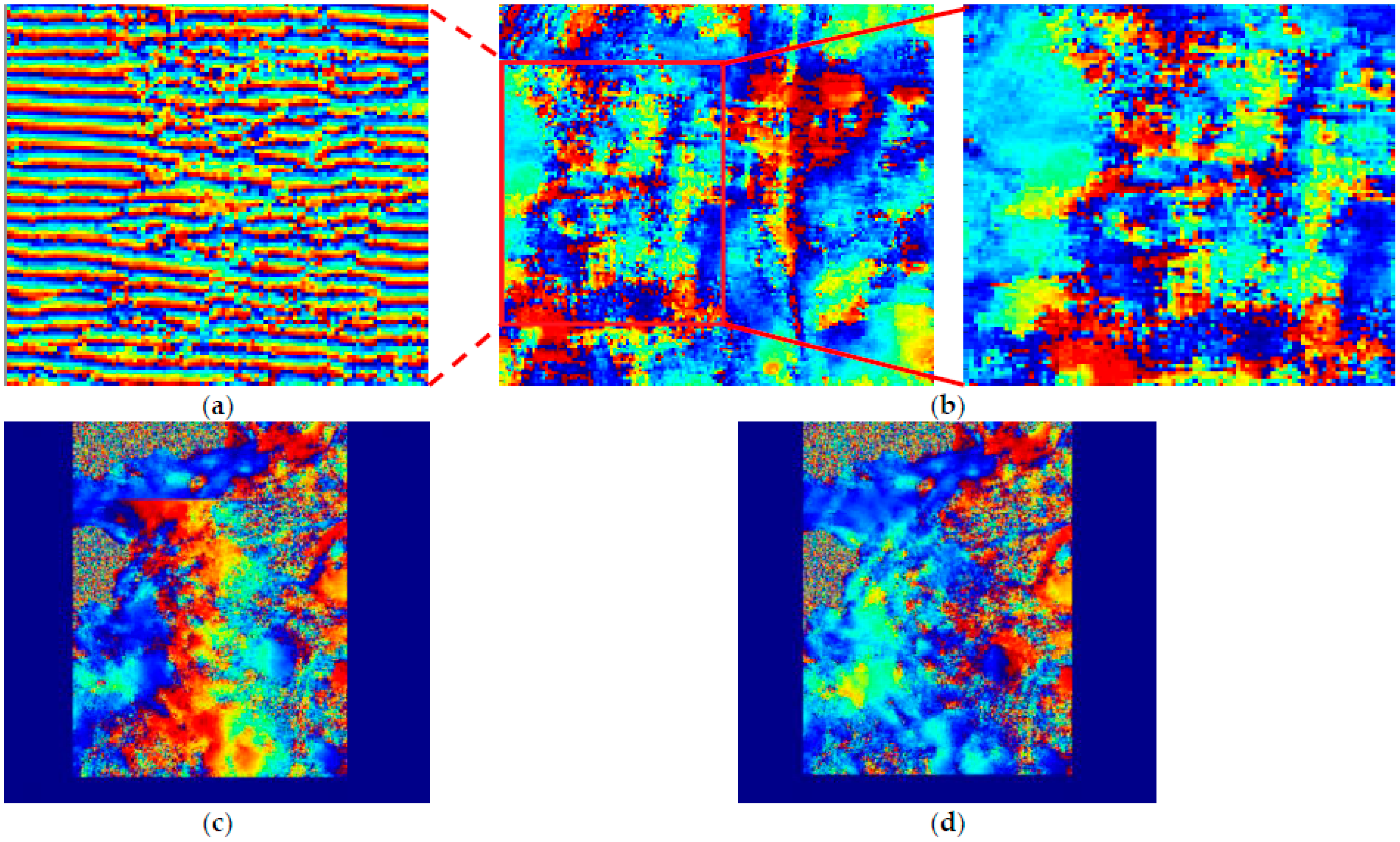
3.1. Characteristics of Residual Fringes Caused by Baseline Errors

Due to the limited application scenarios of the frequency-based flattening method, the orbit-based flattening method is chosen for the initial flattening in this paper. The orbit information provided by the InSAR system will be used to calculate the flat-earth interferometric phase. However, if the orbit information provided by the InSAR system is inaccurate, the inaccuracy will be introduced into the flattened interferogram, resulting in residual fringes. Before removing residual fringes, the characteristics of the fringes will be studied.

According to reference [42], the modulation error in azimuth can be demonstrated clearly because its variation tendency is basically in line with the parallel baseline change and the “slope” error in the range can be obtained directly. In addition, the corresponding slope is given below:

$$k_{tilt}=\frac{\Delta h_{far}-\Delta h_{near}}{R_{far}\sin {\theta }_{far}-R_{near}\sin {\theta }_{near}}=\frac{\Delta B_{\parallel }}{B_{\perp }}$$

(8)

where $\Delta B_{\parallel }$ denotes parallel baseline error, $B_{\perp }$ denotes the vertical baseline, $R_{near}$ and $R_{far}$ denote the proximal and distal distance, respectively, ${\theta }_{near}$ and ${\theta }_{far}$ indicate the proximal and distal angles of view, $\Delta h_{far}-\Delta h_{near}$ is the difference between the proximal and distal elevation, and $R_{far}\sin {\theta }_{far}-R_{near}\sin {\theta }_{near}$ represents the distance between the proximal and distal distance.

In addition, according to reference [37], the errors of baseline length and baseline tilt angle tend to be time-varying considering the limited precision of the twin satellite-mounted navigation systems and the uneven baseline changes caused by the helix formation of the TanDEM-X bistatic system. Without loss of generality, the time-varying characteristic of the baseline error can be extended to more InSAR platforms and systems with inaccurate orbit information.

There are two examples of flattened interferograms using the orbit-based flattening method, as shown in Figure 1, and the InSAR data are provided by the GaoFen-3 system with the imaging modes of Fine Stripe I (FSI) and Fine Stripe II (FSII). As can be seen from Figure 1, the residual fringes are sparse and conform to the first- or second-degree polynomial model locally. In addition, the slop characteristic along the slant range direction is almost non-existent because of the initial flattening, while the density of the residual fringes changes along the azimuth direction, which reflects the characteristic of the time-varying described in reference [37,42]. In addition, the density of residual fringes in Figure 1a changes from dense to sparse along the azimuth direction, while the density of residual fringes in Figure 1b changes from sparse to dense, then sparse and finally dense along the azimuth direction. It means that the time-vary residual fringes are irregular in the whole image and cannot be removed by a polynomial model of the whole image.

Based on the above analysis, three characteristics of residual fringes in the flattened interferogram, which are caused by orbit error, can be obtained as below:

• The residual fringes conform to the first- or second-degree polynomial phase model locally;
• Residual fringes are time varying in azimuth;
• The time varying of residual fringes is irregular in the whole image.

Because of the above characteristics, the traditional refinement and re-flattening methods based on the whole image are no longer applicable. Therefore, considering that the residual fringes conform to the second-degree polynomial phase model in a local area, the idea of the local residual fringe removal is introduced into re-flattening, and the polynomial re-flattening method is adopted in this paper. In addition, adaptive adjusting local windows are designed for the irregularity of the residual fringes.

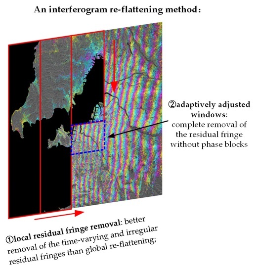
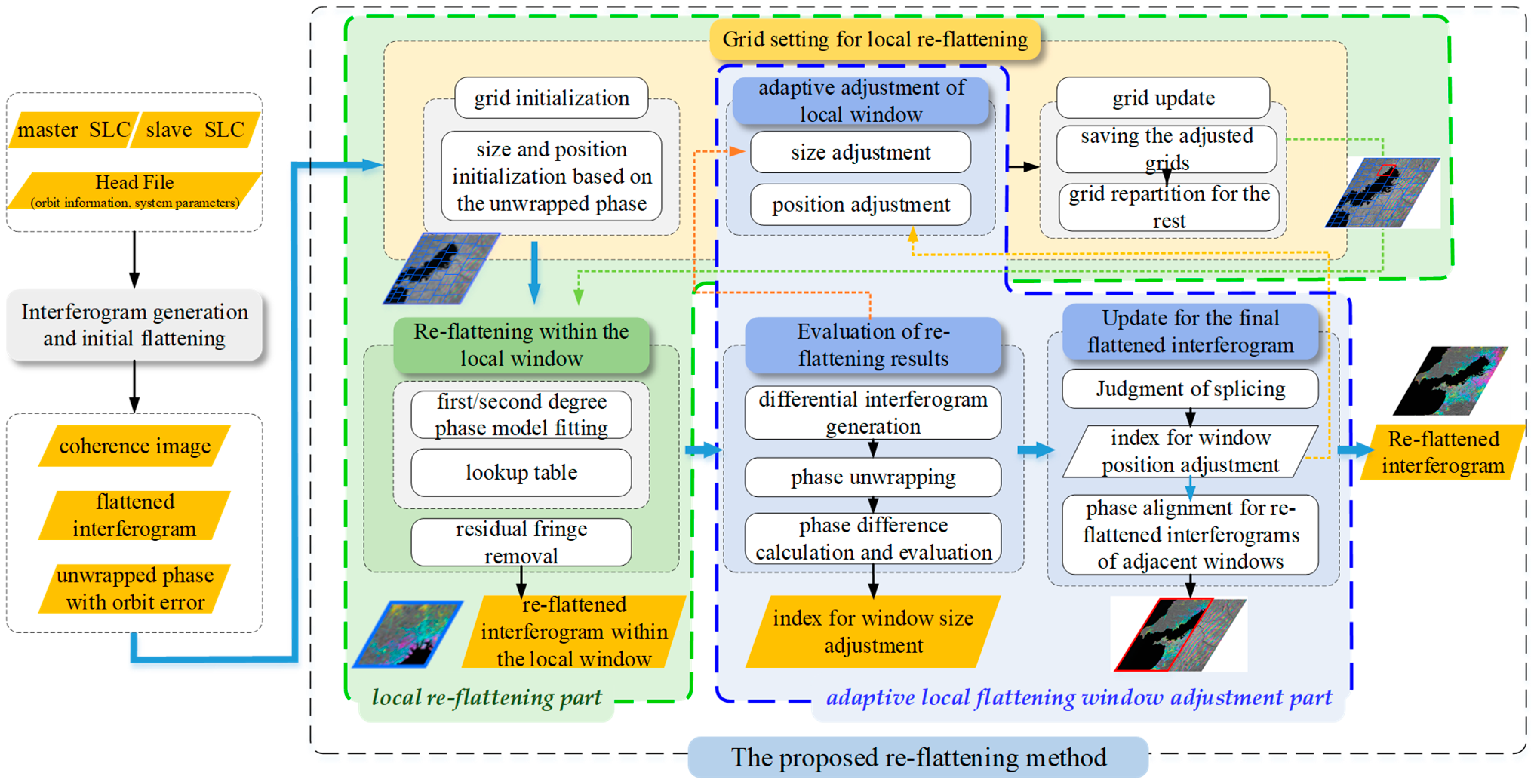
3.2. The Proposed Method: A Re-Flattening Method Based on Local Residual Fringe Removal and Adaptively Adjusted Windows

Based on the above analysis, to obtain the correct terrain interferometric phase, a re-flattening method based on the local residual fringe removal and adaptively adjusted windows was proposed in this paper. In this method, there are two key points: one is the re-flattening in a local window, and the other is the adaptive adjustment of the local window.

To better explain the proposed method, a detailed flowchart is provided in Figure 2. The whole flowchart can be divided into three parts: (1) the interferogram generation and flattening part, (2) the local re-flattening part, including the setting of the local window and the re-flattening within the local window, and (3) the adaptive local flattening window adjustment part, including the evolution of the re-flattening results, the splicing of results between adjacent window, the judgment whether the window position and size are adjusted or not, and the adaptive adjustment of the local window.

For the interferogram generation and flattening part, a pair of InSAR data and their head files are input for co-registration, interferogram generation, flattening, filtering and phase unwrapping, and finally, the coherence image, the flattened interferogram and the unwrapped phase are obtained for subsequent processing. There are many excellent algorithms for each step [43,44,45,46,47], among which Goldstein method [43,44] is adopted for filtering, and Minimum Cost Flow method [45] is adopted for phase unwrapping.

Phase unwrapping was performed on the flattened interferogram with residual fringes, and the variation characteristic of the residual phase can be obtained more directly and clearly from the unwrapped phase image, which can be used for subsequent processing.

The other two key parts will be elaborated on below.

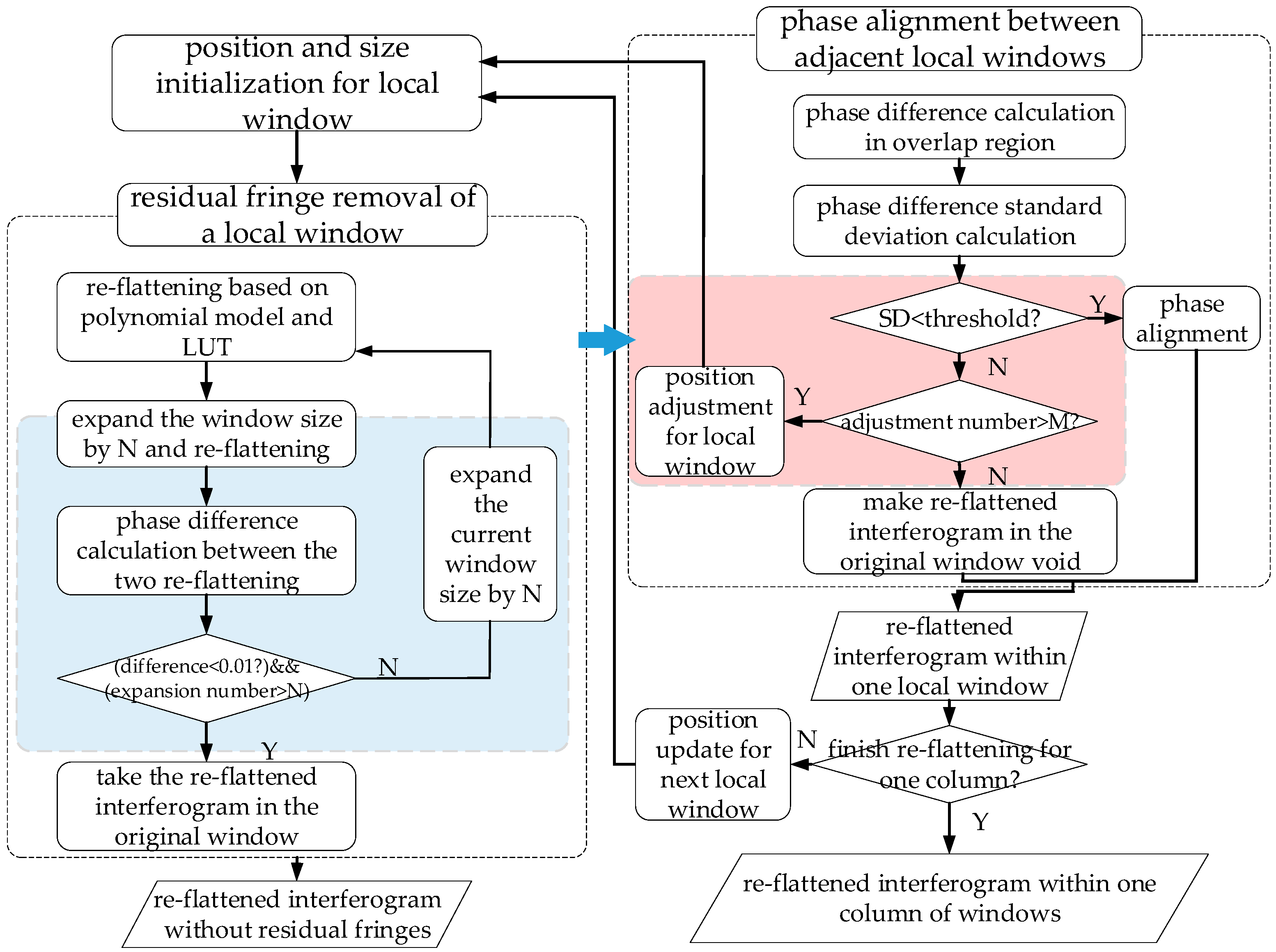
3.2.1. Principle of the Re-Flattening within A Local Window

Based on the analyses of the residual phase in Section 3.1, the second-degree polynomial phase model in Equation (2) is used to calculate the residual phase.

To avoid the inaccurate estimation of polynomial coefficients, which is based on several GCPs, the LUT method is introduced into the residual phase estimation within a local window. The LUT contains six parameters, which are $f_a$, $f_r$, $f_{2a}$, $f_{2r}$, $f_{ar}$ and $C$. In LUT, the interval of $f_{2a}$ and $f_{2r}$ will be set according to the minimum and maximum second-order phase gradient, and the length of the step is set as 0.001; the interval of $f_a$, $f_r$ will be set according to the minimum and maximum phase gradient, and the length of step is set as 0.01; the interval of C will be set according to the minimum and maximum phase, and the length of step is set as 0.01. The calculated phase will be compared with the interferogram with residual fringes, and when the phase difference is less than 1 rad or the phase difference is minimal, the calculated phase will be chosen and subtracted from the interferogram with residual fringes.

In addition, to avoid the inaccurate caused by low coherence, the points with coherence less than 0.6 will not be considered in the residual phase estimation within a local window.

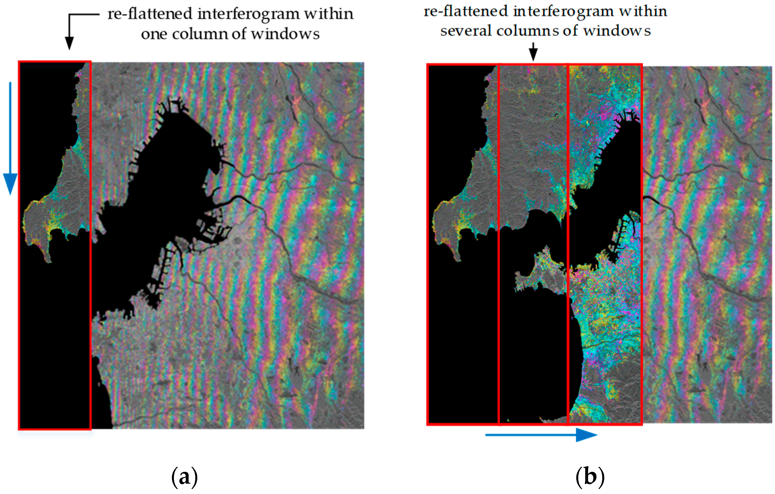
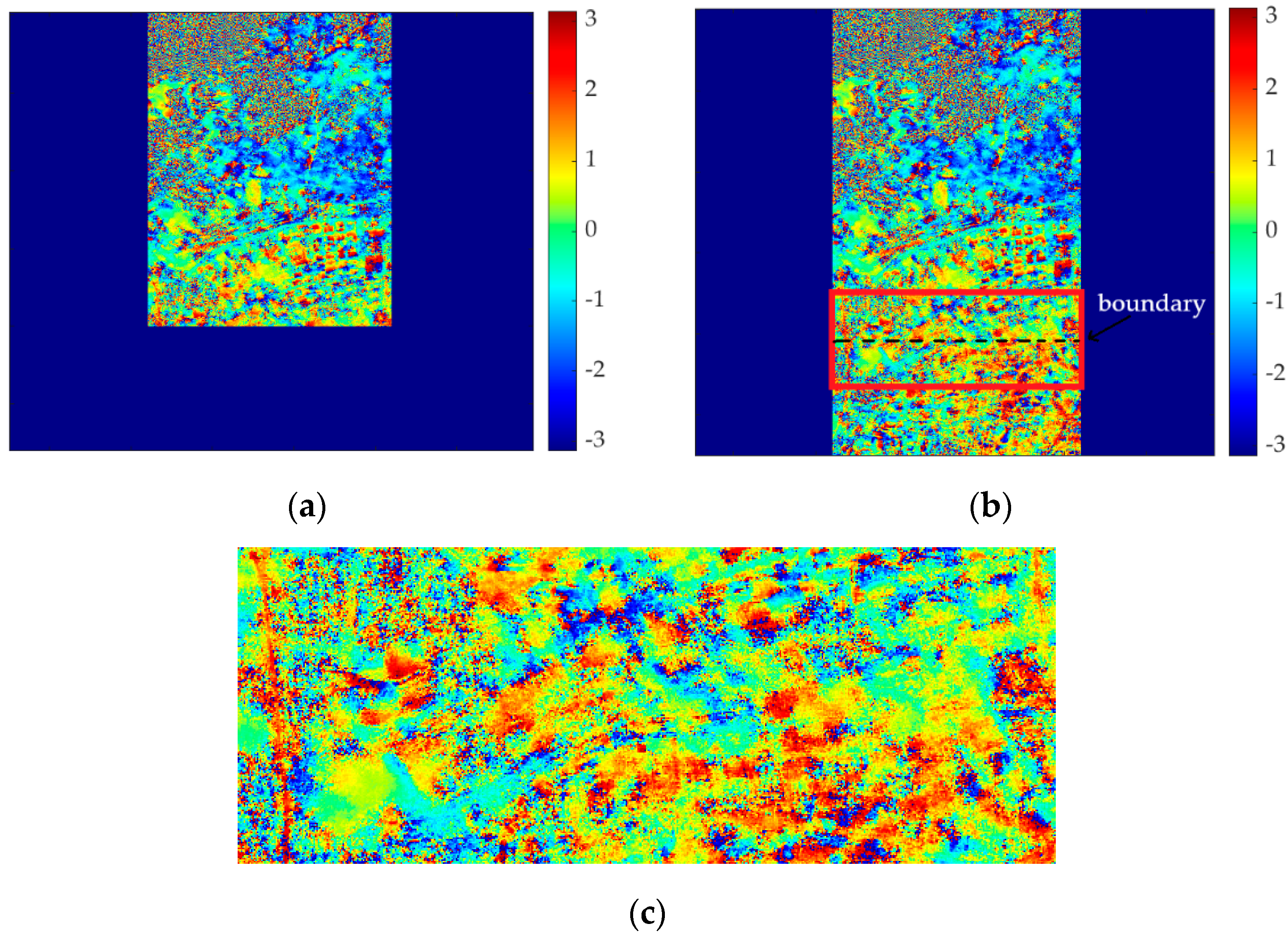
3.2.2. Mechanism of Adaptive Adjustment for Re-Flattening Windows

Before re-flattening, the position of the current window will be set and initialized. In addition, to avoid the blocking effect caused by local processing, the overlap is set between adjacent windows. Then, the size of the window will be initialized, and the operation will be performed on the unwrapped phase image to obtain a clearer phase gradient variation. The size of the local window is determined by a fixed phase gradient difference. The position set in the previous step is used as the reference point, and when the phase gradient changes by a threshold, the position here is selected as the end point of the window. In this paper, the threshold of the phase gradient difference usually is set as 0.01 based on experience, which ensures the similarity of the residual fringes in the local window.

As the re-flattening, the evaluation of the re-flattening results, the adjustment of the local window and the update of the final flattened interferogram are closely related, they will be described together as the mechanism of adaptive adjustment for re-flattening windows, and the detailed flowchart is shown in Figure 3.

After the above step, the local window is determined initially, and the residual fringes within the local window will be removed after the re-flattening based on the principle in Section 3.2.1. However, because of the local processing, there is usually a phase difference between the re-flattened interferogram of adjacent windows. Therefore, the phase alignment between adjacent windows must be performed, and the phase difference in the overlay area can be used as the phase difference between adjacent windows.

To avoid the influence of phase discontinuity on phase alignment, which is usually caused by abrupt topography or low coherence, two methods are adopted in this paper. The points with discontinuous phases will cause a large phase difference, which is different from other points, and when calculating the phase difference between adjacent windows, outliers will be removed to avoid the effect of phase discontinuities. In addition, when there are too many discontinuous phase points, the phase difference between adjacent windows will be particularly large. At this time, the phase difference will not be adopted, and the window will be adjusted to avoid this situation.

Improper position and size of the local window will result in residual fringes not being completely removed, and then the phase alignment cannot be performed because of a large standard deviation of the phase difference. The key point to solving this problem is to choose an appropriate position and size for the local window. Adaptive size adjustment and position adjustment modules are proposed, as shown in the blue part and red part in Figure 3, respectively.

Part of the experimental results of Gaofen-3 InSAR data will be used to illustrate the importance of size and position adjustment for re-flattening windows and local re-flattening, as shown in Figure 4.

When the window is too small, the re-flattening will be affected by the local terrain phase, thus introducing new phase errors, as shown in Figure 4a. In this paper, shown in the blue part in Figure 3, the re-flattened interferogram within the current window will be compared with that in the expended window, and if the difference between them is greater than the threshold, the current window will be considered too small and will be replaced by the expanded window. Repeat the above step until a suitable window is obtained, and to avoid infinite loops, the maximum number of window expansions is set. The purpose of the above processing is to avoid the local optimum problem of the phase fitting, which means the residual fringes cannot be removed cleanly. After this step, the re-flattened interferogram without the residual fringes can be obtained correctly, as shown in Figure 4b.

Improper position of the window may also result in residual fringes not being completely removed, as shown in Figure 4c. Aiming at this problem, shown in the red part in Figure 3, the standard deviation of the phase difference between adjacent windows is used as an indicator, and when the standard deviation is greater than the threshold, the current window position is considered to be inappropriate and will be adjusted upward. The re-flattening will be performed within the new window, and the standard deviation will also be recalculated. Repeat the above step until a suitable position is obtained, and then the interferograms of adjacent windows can be aligned as shown in Figure 4d. Additionally, to avoid infinite loops, the maximum number of position adjustments will be set.

If the condition of phase alignment cannot be satisfied after the adaptive adjustment of position and size, the re-flattened interferogram in the original window will be set to be void. The reason is that the residual fringes do not conform to the second-degree polynomial phase model, and the void part will be re-flattened by readjusting the window position and size in the subsequent step.

Based on the above steps, the re-flattening will be finished first in one local window, then in one column of windows, and finally in the whole image, as shown in Figure 5.

4. Experiments

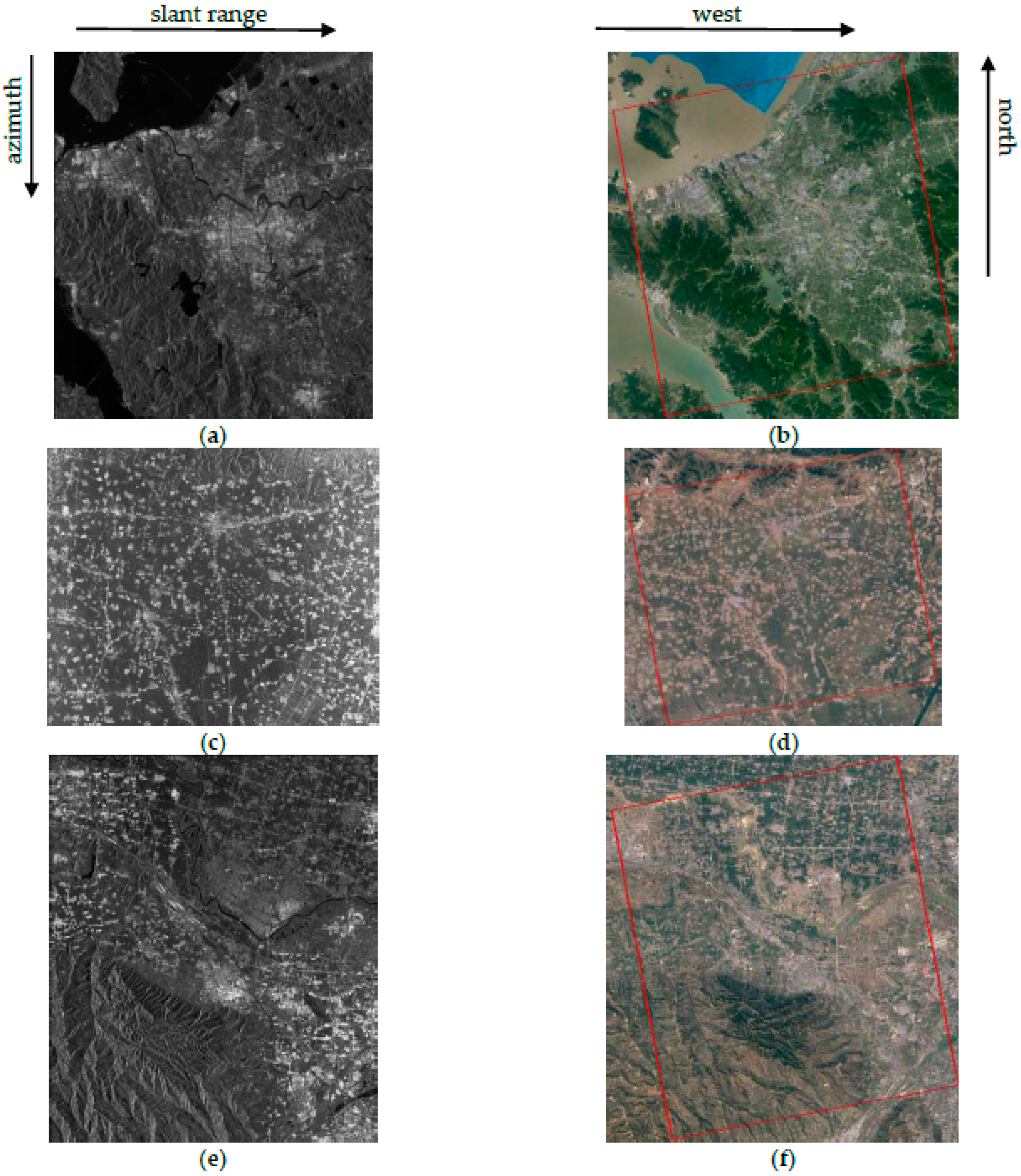
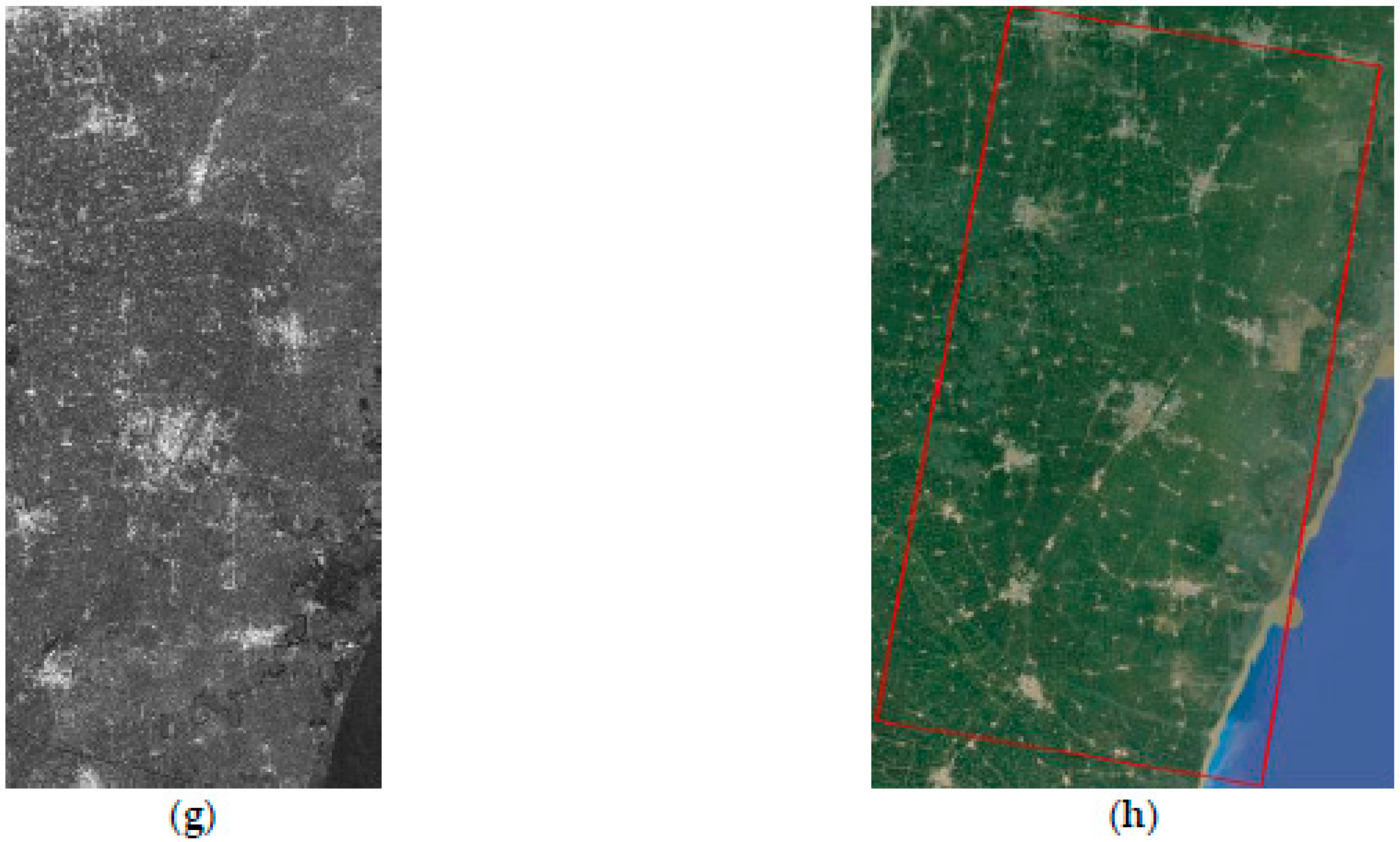
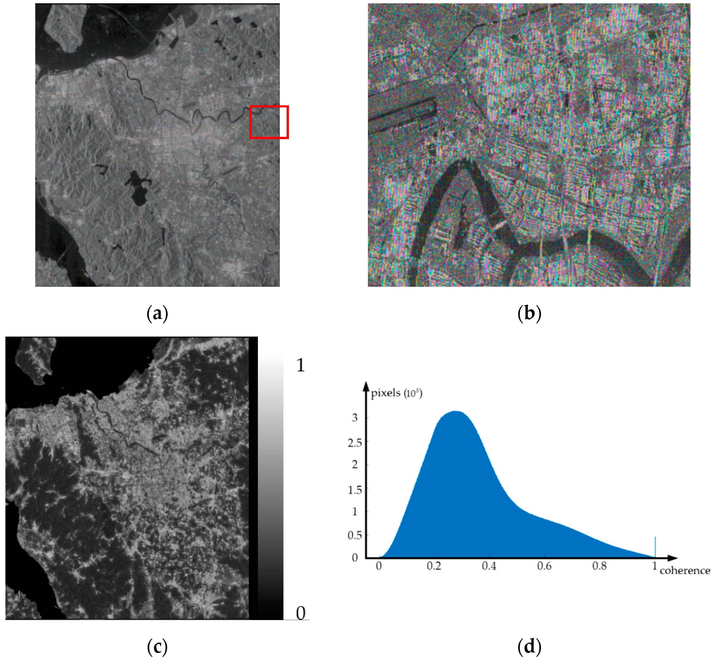
4.1. Experimental Data and Study Area

Three pairs of GaoFen-3 InSAR data and one pair of Sentinel-1A InSAR data were used for experiments, which are located in Ningbo City, China, Yutian County, China, Xi’an City, China, and Yancheng City, China, respectively. SAR intensity images and corresponding optical images of the four pairs of InSAR data are given in Figure 6. As can be seen from Figure 6, there are both flat urban areas and mountainous areas in these four sets of data. Related parameters of these experimental data are shown in

Table 2. Parameters of four InSAR pairs.

	Imaging Mode	Polarization	Resolution (Azimuth × Slant Range)	2π Ambiguity Height
GF-3 InSAR data in Ningbo	Fine Strip I	HH	2.86 × 3.31 m	31.05 m
GF-3 InSAR data in Yutian	Fine Strip I	HH	3.13 × 3.61 m	62.55 m
GF-3 InSAR data in Xi’an	Quad-Polarization Strip I	HH	5.54 × 3.80 m	109.98 m
Sentinel-1A InSAR data in Yancheng	IW	HH	13.92 × 23.30 m	224.12 m

, and as can be seen from it, the experimental data with different parameters are chosen to obtain the accuracy of the proposed method under different data conditions.

The re-flattening method proposed in this paper will be compared with the commonly used refinement and re-flattening methods in Section 2, that is, the global polynomial refinement method (GPR method), the second-degree baseline error model-based refinement and re-flattening method (SBDR method) and the re-flattening method based on local frequency estimation (using the manually designed windows) (LFE-MW method).

Two evaluation methods will be used: one is qualitative evaluation, and the other is quantitative evaluation. In qualitative evaluation, the evaluation method is to observe whether there are residual fringes after re-flattening and whether the re-flattened interferometric phase can correctly reflect the terrain. In quantitative evaluation, the DEMs will be obtained based on the re-flattened interferograms and were used to indirectly reflect the performance of the proposed method. The difference between the generated DEMs and the reference SRTM DEM will be used as the evaluation index, including the mean absolute error (MAE) and root mean square error (RMSE). In addition, the indicators of the relative increase in MAE and RMSE (∆MAE and ∆RMSE) have also been used for the relative comparison. Further, if buildings can be clearly reflected in the re-flattened interferogram, the accuracy of the building height estimation in simple scenarios will also be used as one of the evaluation indicators.

The InSAR pair located in Ningbo City is taken as a representative to give a detailed explanation of the experiment. For the other data, only the final re-flattened interferograms and DEMs, as well as accuracy analysis, are given.

The interferogram and the coherence image of the InSAR data in Ningbo City are shown in Figure 7, and to reduce the influence of the speckle noise, a 4 × 4 multi-look processing was adopted. It can be seen from Figure 7a,b that there are very dense fringes in the interferogram. As shown in Figure 7c, the coherence is about 0.5 to 0.7 in the urban area, while it is below 0.3 (even below 0.2) in mountains, and the average coherence of the whole image is 0.35.

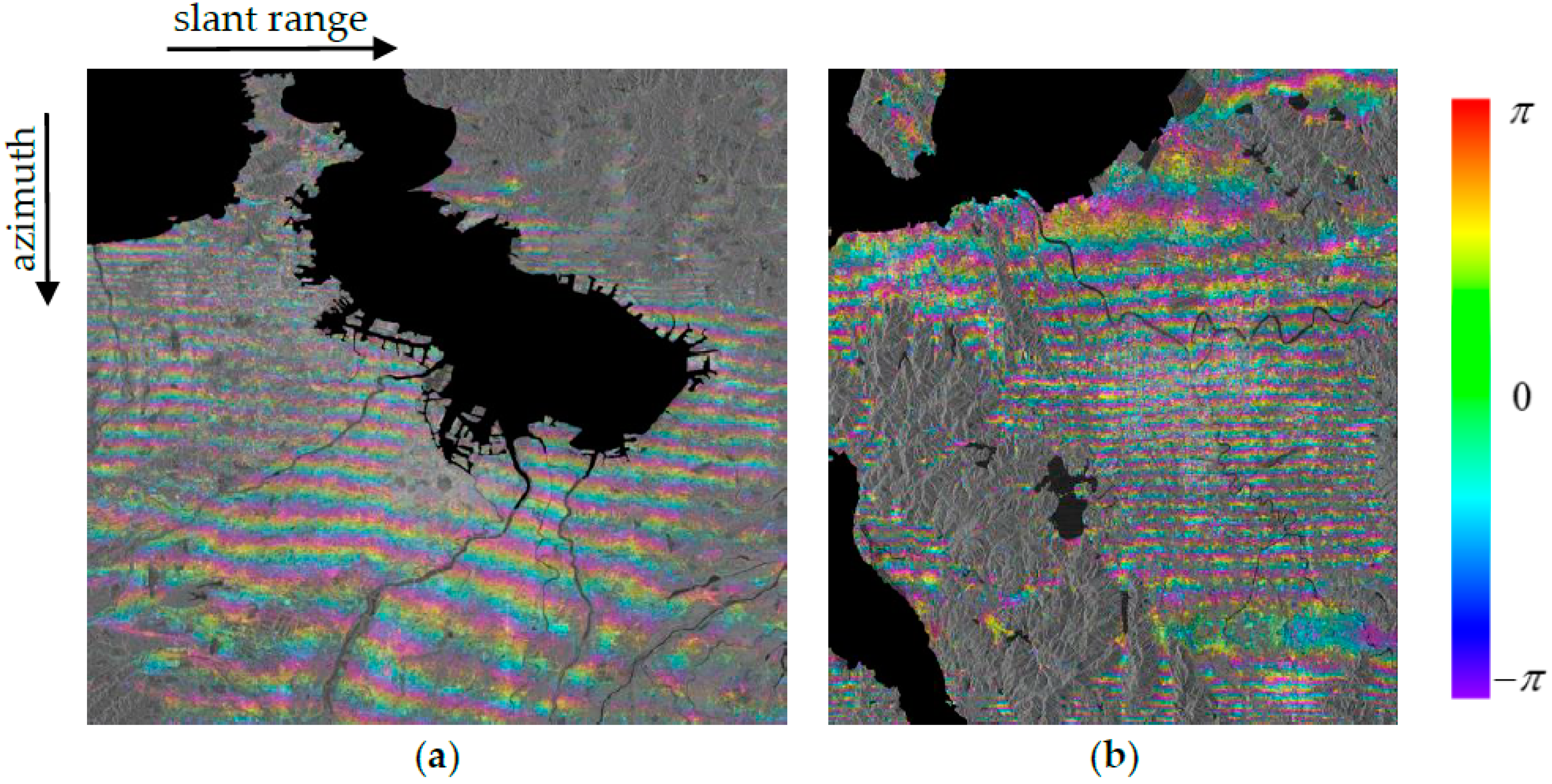
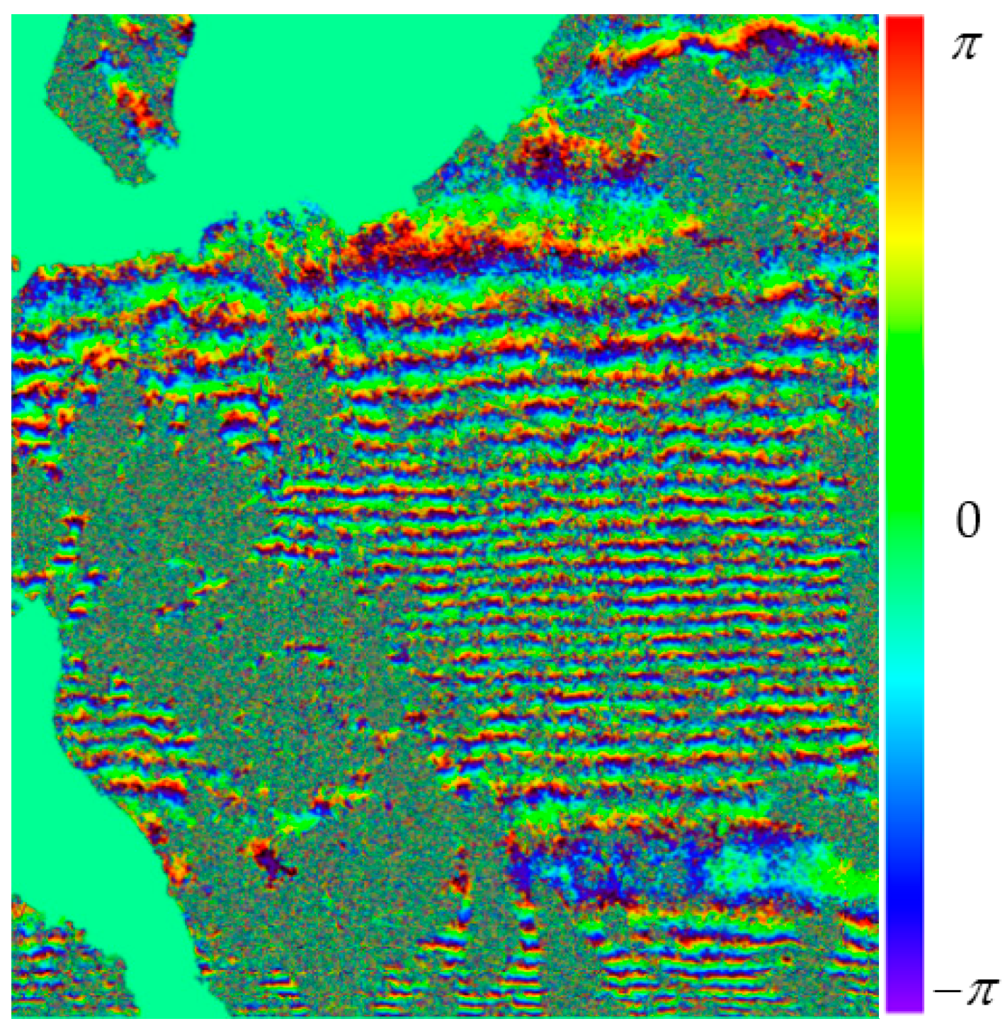
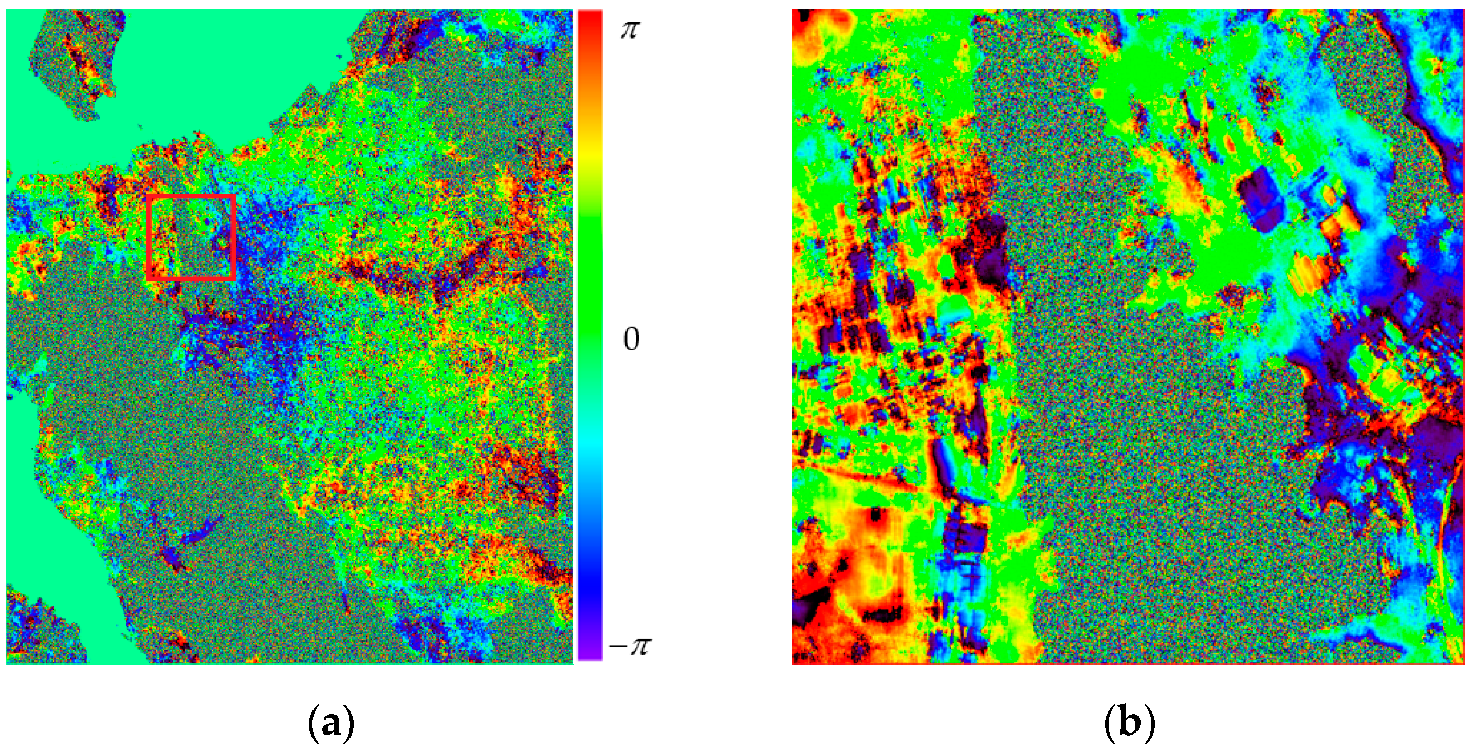
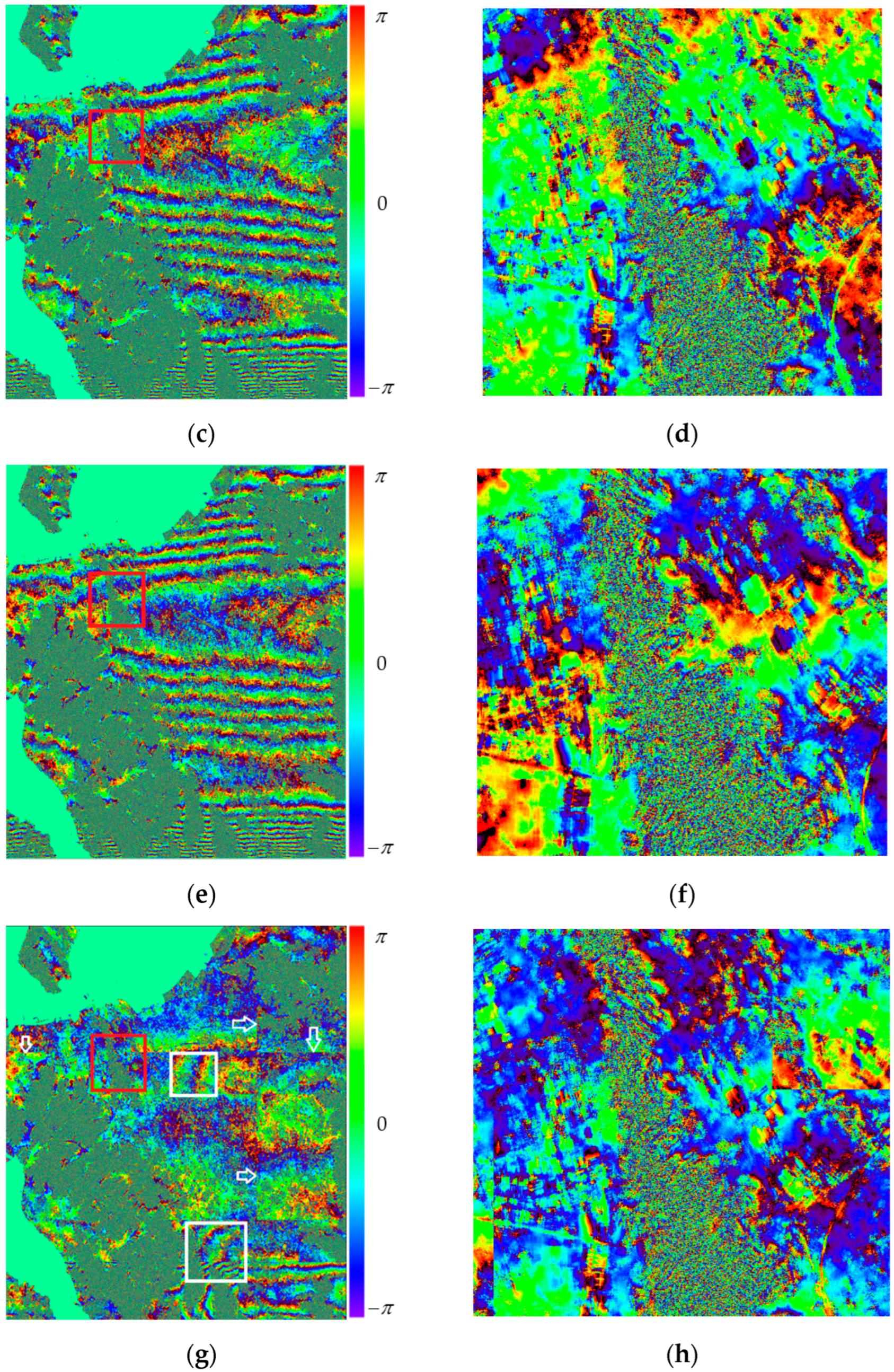
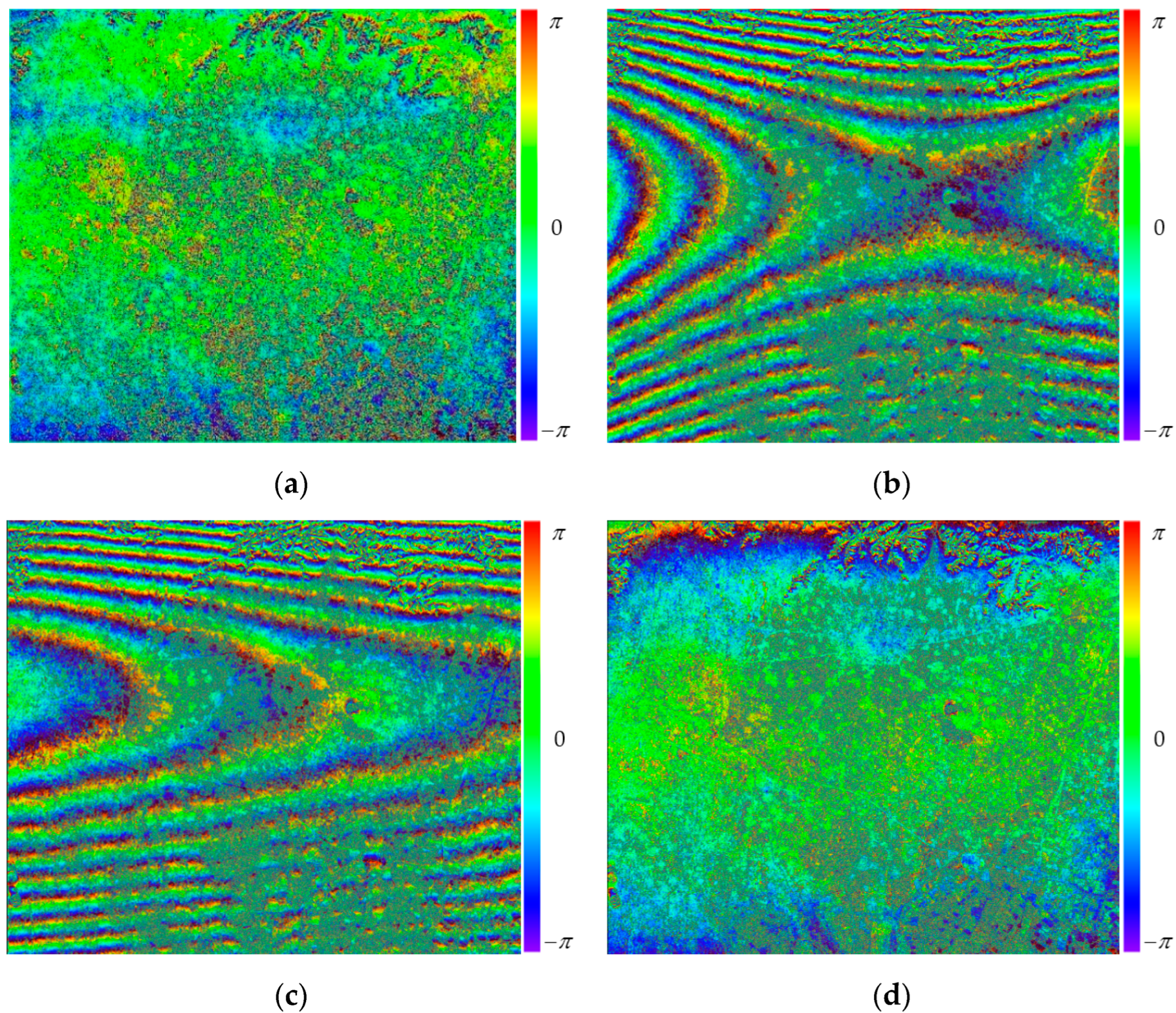
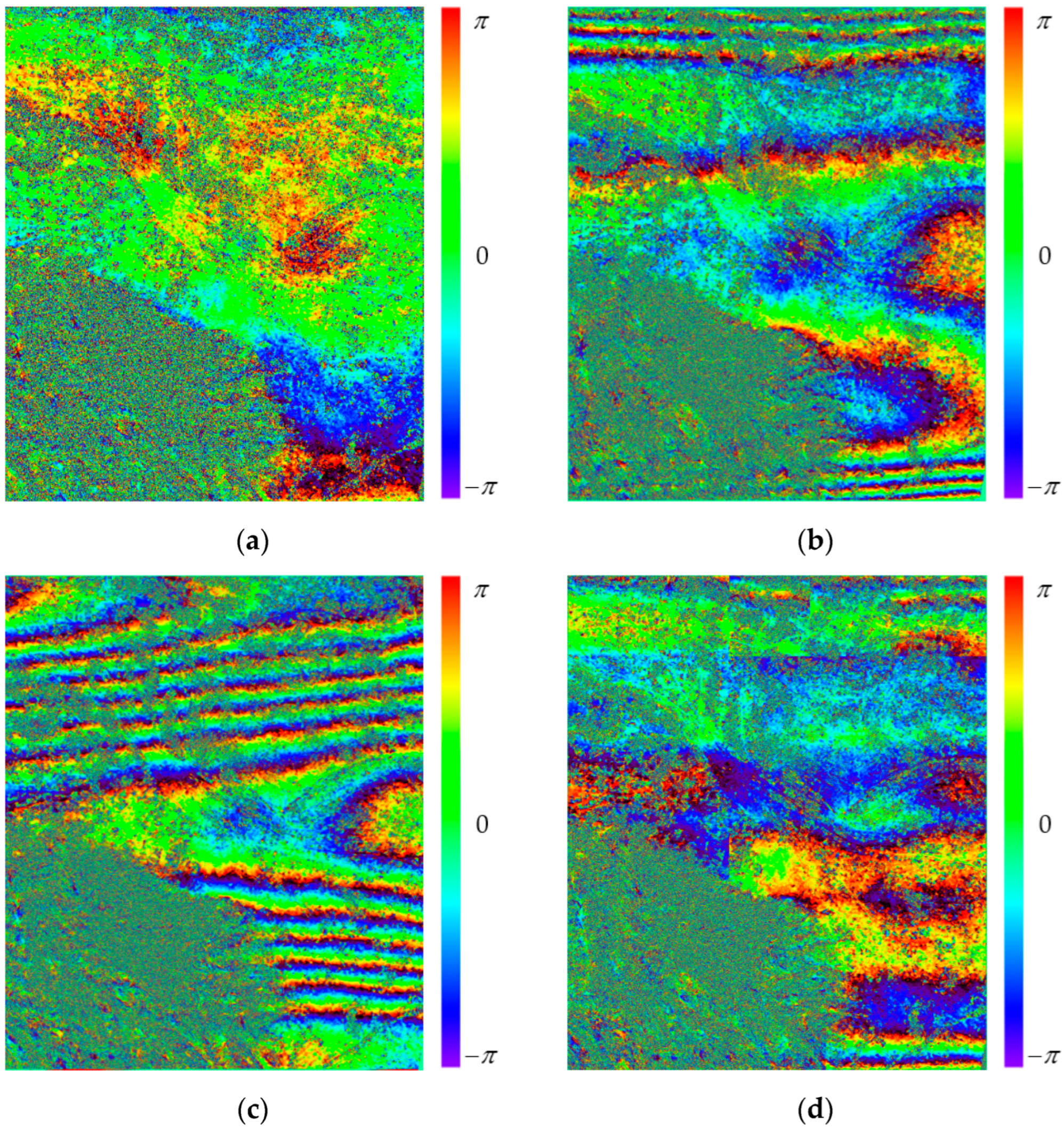
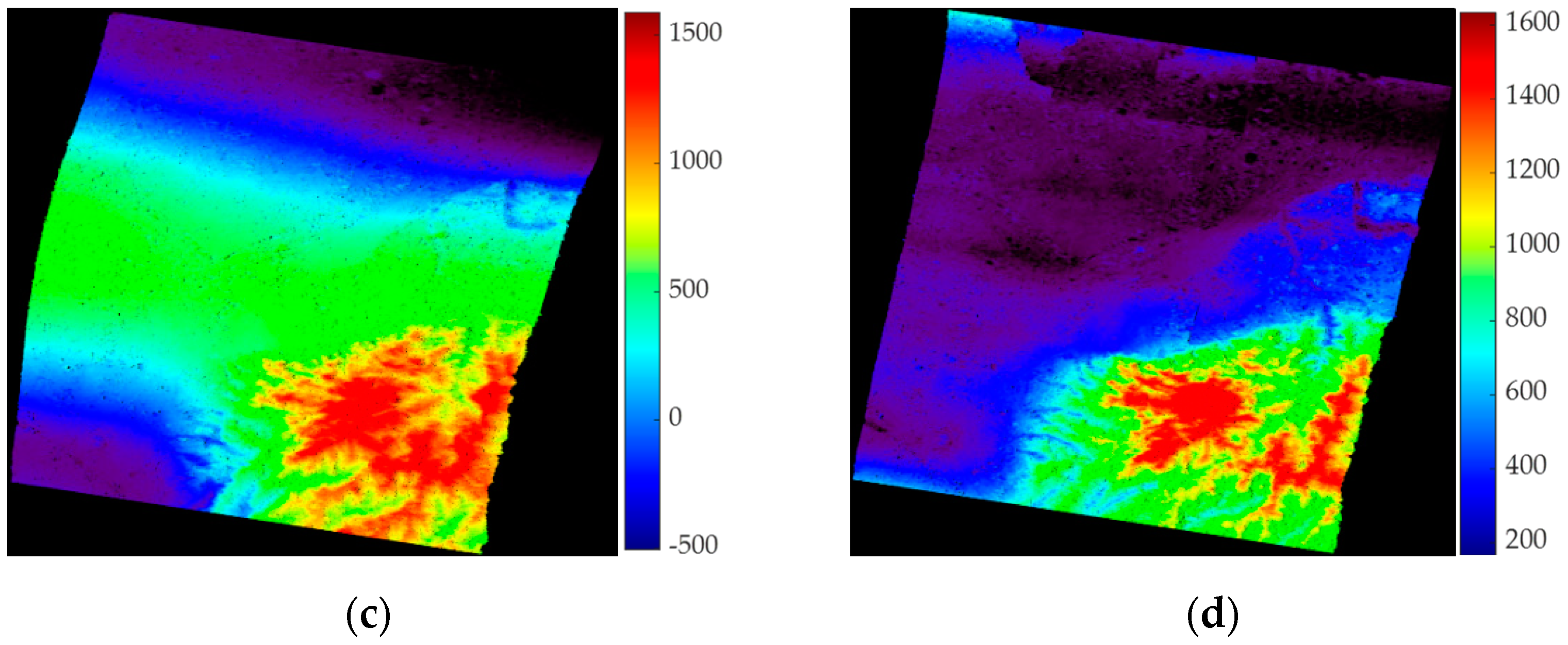
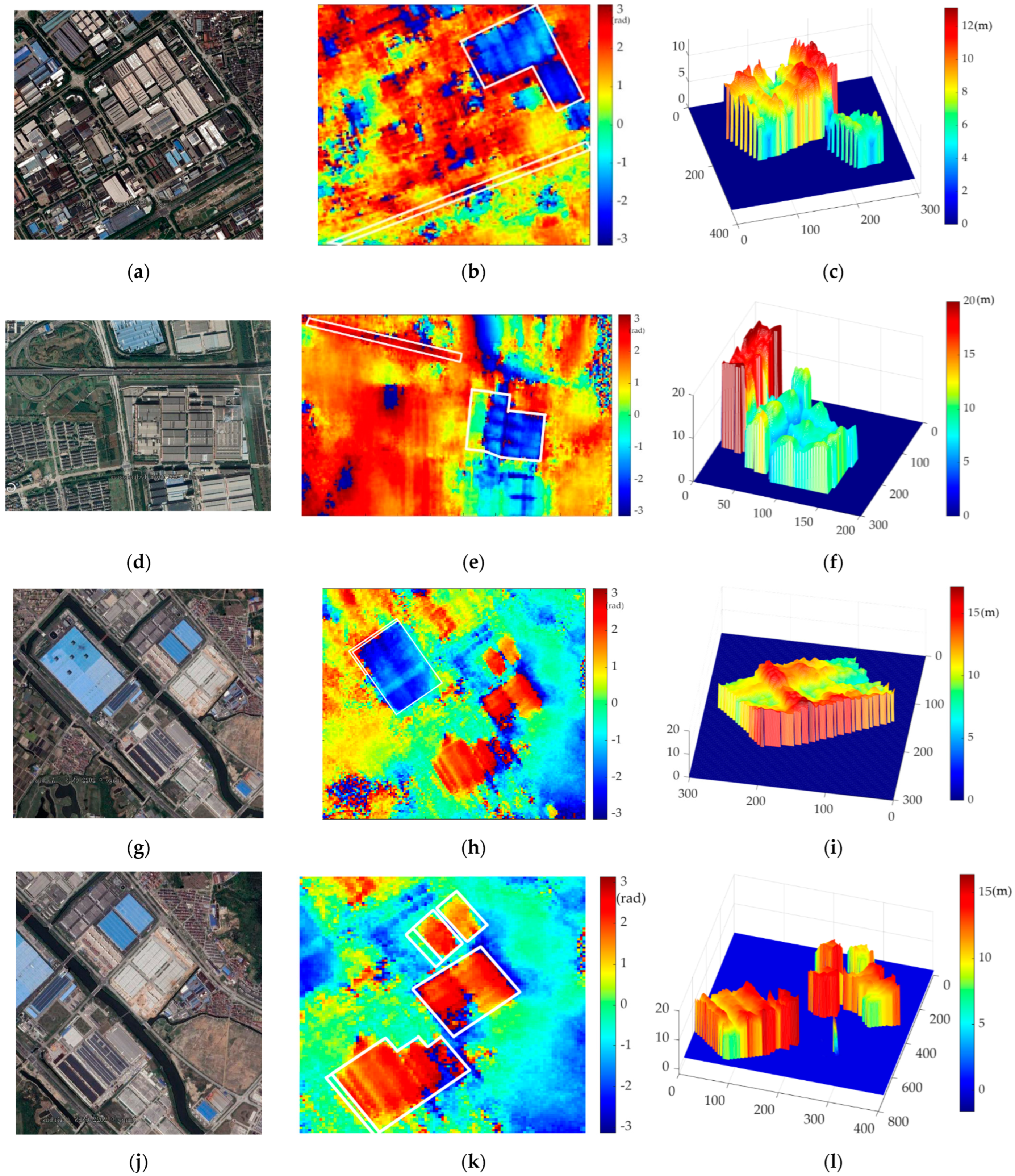
4.2. Re-Flattening Results and Qualitative Evaluations

The orbit-based flattening method was applied to the InSAR data, and the flattened interferogram is shown in Figure 8. As can be seen from it, there are residual fringes in the flattened interferogram, and the density of the residual fringes changes along the azimuth direction. From another point of view, there are about 33 residual fringes in the flattened interferogram and the corresponding phase change is about 33 × 2π. Combined with the 2π ambiguity height of 31.05 m, the terrain change reflected in the image is about 1025 m, which is very inconsistent with the actual terrain. Therefore, the re-flattening was performed to obtain the correct terrain interferometric phase and DEM.

The re-flattening was performed based on the proposed method in this paper, and the detailed results of the local re-flattening and the phase alignment are shown in Figure 9. The interferogram in Figure 9a has been re-flattened and aligned, and based on it, the re-flattening and phase alignment of the next window are performed and the interferogram in Figure 9b is obtained. It can be seen from Figure 9a,b that there is no residual fringe in the re-flattened interferogram. In addition, the re-flattened interferogram at the boundary of adjacent windows is enlarged as shown in Figure 9c, and it can be seen that the interferometric phase at the boundary is continuous, and there is no blockiness. The results in Figure 9 show that the method proposed in this paper is effective in the removal of residual fringes.

To illustrate the effectiveness and accuracy of the proposed method in this paper, it is compared with the above-mentioned refinement and re-flattening methods. The re-flattened interferograms are shown in Figure 10.

For the GPR method and SBDR method, several GCPs are selected to solve the parameters of the residual phase model or the baseline error model. However, for the flattened interferogram with unevenly varying residual fringes, the residual phase at the selected GCPs does not fully represent that of the whole image, and then the estimated residual phase or the baseline error is inaccurate for the whole image. Therefore, the residual fringes cannot be removed completely for GPR and SBDR methods, as shown in Figure 10c–f. With reference to the reference [38], smaller windows are set on steep terrain, and larger windows are set on flat terrain, and then the LFE-MW method is executed. The window was resize twice based on the results, and the result is shown in Figure 10g,h. Only from analyzing the results of each local window, the residual fringes in Figure 10g are removed more cleanly, compared with Figure 10c,e. Additionally, this also proves the effectiveness of local re-flattening. However, from the perspective of the whole image, the result in Figure 10g has the problems of the incomplete interference fringe removal in individual windows shown as the white rectangular box in Figure 10g and the obvious blocky effect between adjacent windows shown as the white arrow in Figure 10g. The reason is that the removal of residual fringes is very sensitive to the window setting, and manually set windows are difficult to meet the need, especially for large scene images with complex residual fringes. In addition, a lot of time and effort needs to be spent on adjusting the windows, if the above problem is wanted to be solved.

The re-flattened interferogram and its detail based on the proposed method in this paper are shown in Figure 10a,b. Compared with the interferogram in Figure 10c, there are almost no residual fringes in the interferogram in Figure 10a, and compared with Figure 10g, the residual fringes in each window are removed in Figure 10a, and there is no blocky effect in the whole image. In addition, combined with the ambiguity height, the re-flattened interferogram in Figure 10a can roughly reflect the correct terrain, and as can be seen from the enlarged image in Figure 10b, some roads and buildings can be clearly reflected in the image.

The re-flattened interferograms of the other InSAR data are shown in Figure 11, Figure 12 and Figure 13. The interferograms in Figure 11a, Figure 12a and Figure 13a are based on the re-flattening method proposed in this paper, and compared with other results, it can be seen that the residual fringes are cleanly removed in the whole image. The interferograms in Figure 11b,c, Figure 12b,c and Figure 13b,c are the results based on the global re-flattening methods (GPR method and SBDR method). There is a serious problem with the results of this type of method; that is, when the change of residual fringes in the image is complex, they cannot be removed completely. The interferograms in Figure 11d, Figure 12d and Figure 13d are the results based on the LFE-MW method. There are no obvious residual fringes, but the residual fringes have not been completely removed, as shown at the top of Figure 11d and the bottom of Figure 12d and Figure 13d, and there is a blocky phenomenon in the results.

Compared with the other three results, the re-flattened interferograms based on the proposed re-flattening method are better both in the residual fringe removal and the overall effect. It indicates that the proposed method has a better effect on the removal of the residual fringes with time-varying and uneven density.

Based on the above results and analysis, it can be seen that the proposed re-flattening method is more effective in the removal of the residual fringes with time-varying and uneven density, and the corresponding terrain interferometric phase is more accurate, compared with the global re-flattening methods (GPR method and SBDR method) and the manual window-based local re-flattening method (LFE-MW method). In addition to qualitative analysis and comparison, the re-flattened interferograms will be used to generate DEMs, which will be used for quantitative evaluation.

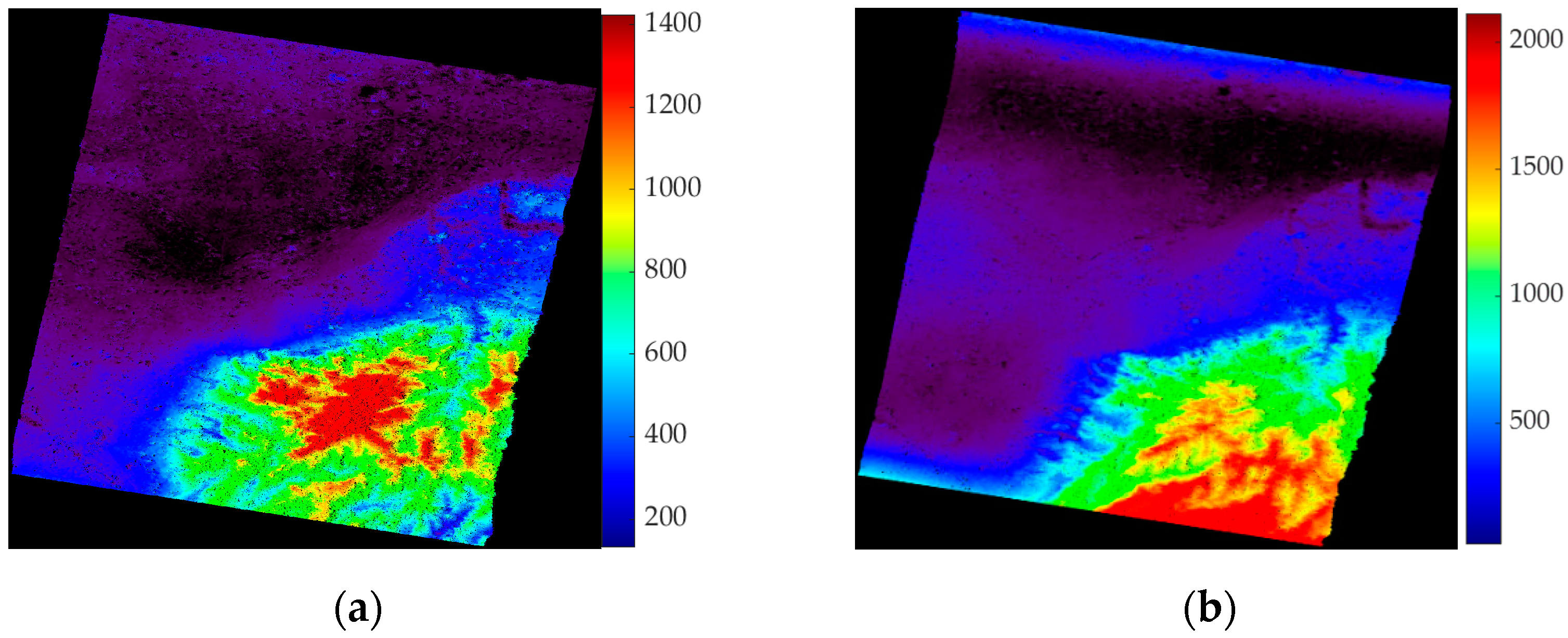
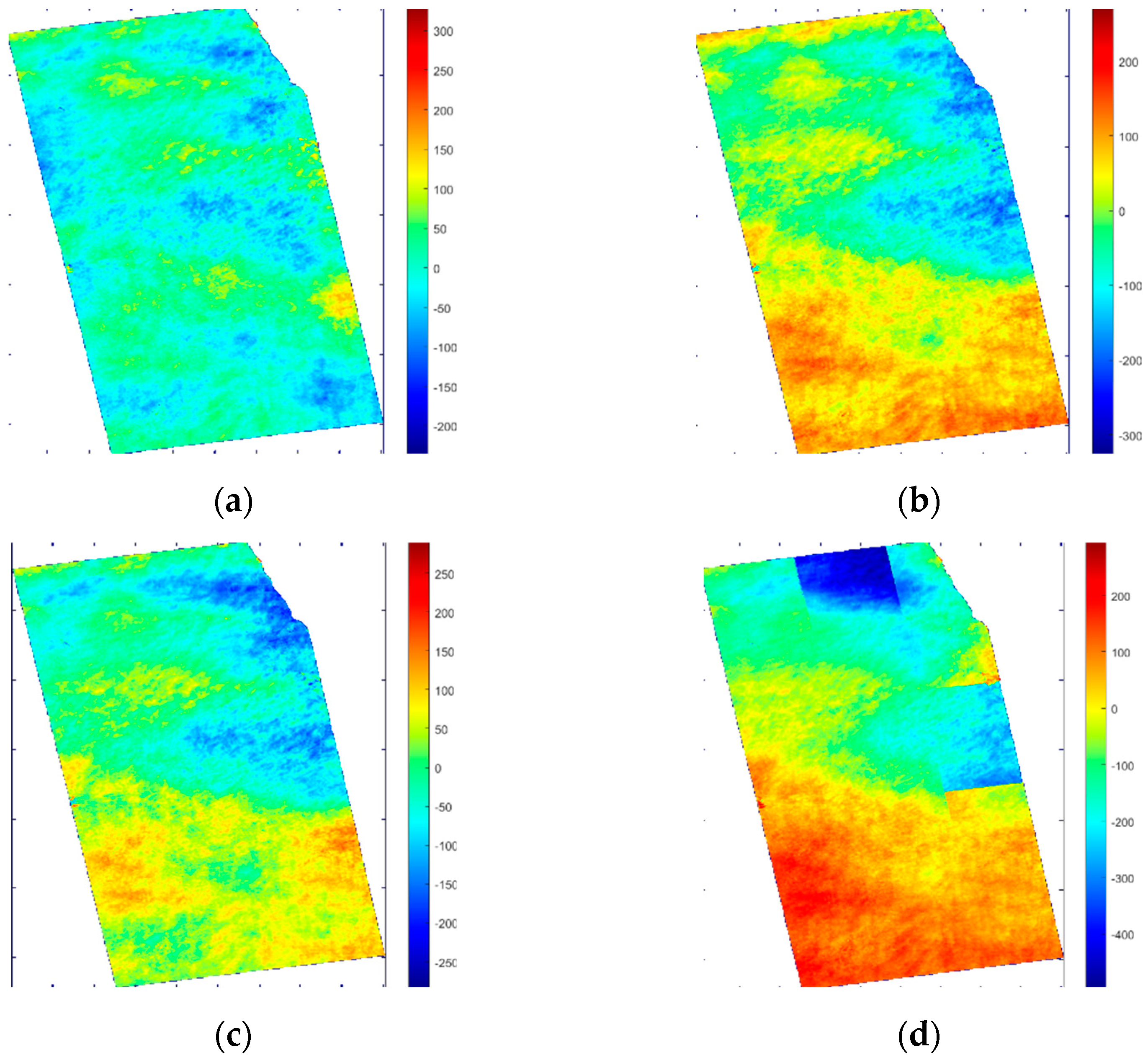
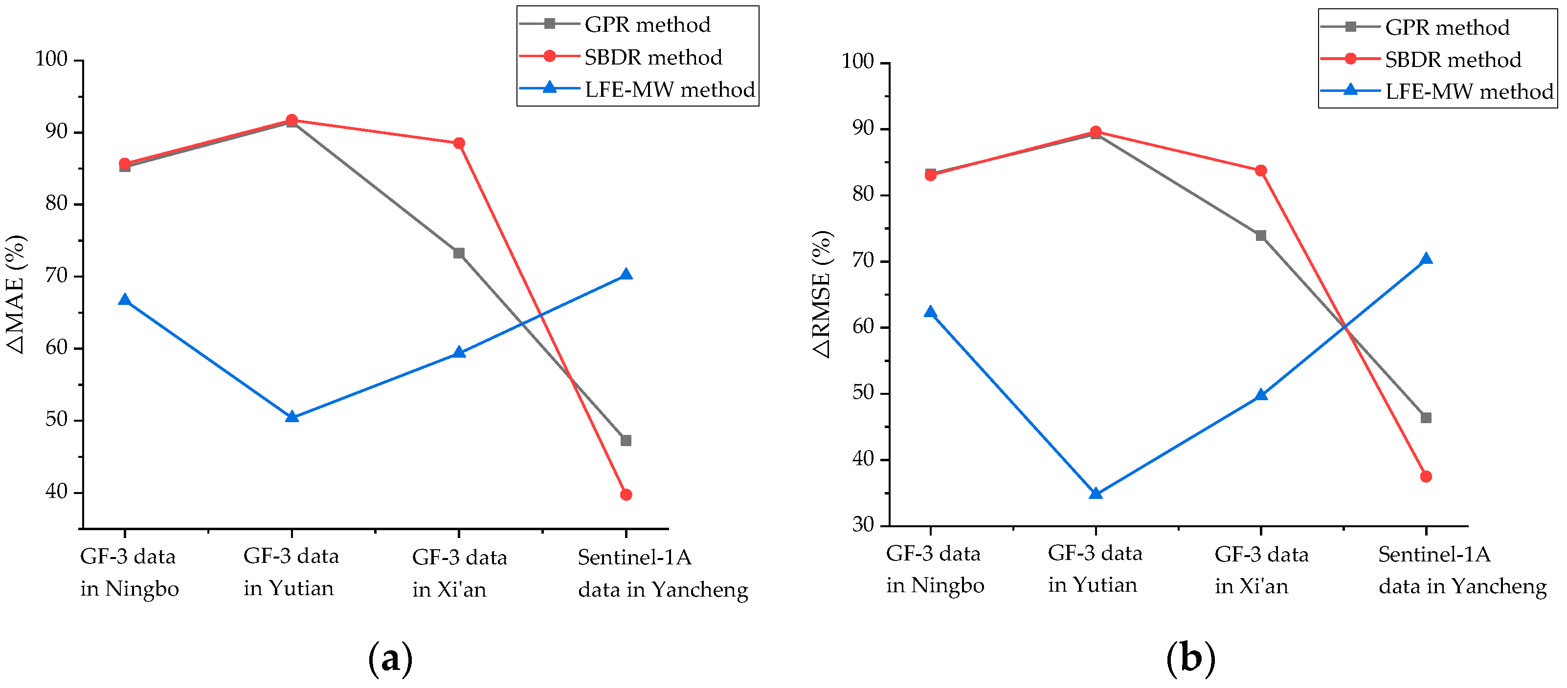
4.3. DEM Generation and Quantitative Evaluation

The generated DEMs based on the re-flattened interferogram obtained in the previous subsection are shown in Figure 14, Figure 15, Figure 16 and Figure 17. As can be seen from these results, DEMs generated by the re-flattened interferograms using the global re-flattening methods (GPR method and SBDR method) do not match the actual terrain, and the stripy DEM error in the image drowns the real terrain in it. In addition, compared with the results based on the global methods, the stripy DEM error is greatly reduced in the results based on the manual window-based local re-flattening method, and the only pity is that there are DEM errors caused by the blocky phase in the results. However, compared with the above three methods, DEMs generated by the re-flattened interferograms using the proposed method are more accurate and consistent with the actual terrain. In addition, there are no stripy and blocky DEM errors in the results.

The corresponding SRTM DEMs are used as the reference DEMs, and the generated DEMs are compared with them to obtain the quantitative evaluation. MAE and RMSE are adopted as evaluation indicators, and they are shown in Equations (9) and (10).

$$MAE=\frac{1}{M\cdot N}{\displaystyle \sum _{i=1}^M{\displaystyle \sum _{j=1}^N\left|\mathrm{DEM}\left(i,j\right)-\mathrm{SRTM}\mathrm{DEM}\left(i,j\right)\right|}}$$

(9)

$$RMSE=\sqrt{\frac{1}{M\cdot N}{\displaystyle \sum _{i=1}^M{\displaystyle \sum _{j=1}^N{\left(\mathrm{DEM}\left(i,j\right)-\mathrm{SRTM}\mathrm{DEM}\left(i,j\right)\right)}^2}}}$$

(10)

where $M$ and $N$ denote the numbers of pixels in azimuth and slant range, respectively; and $i$ and $j$ denote the coordinate of the pixel in the image.

The evaluation of the generated DEMs is shown in

Table 3. DEM evaluation.

Data\Indictor	Average Coherence	$2\mathit{\pi }$ Ambiguity Height (m)	Method	MAE (m)	RMSE (m)
GF-3 InSAR data (Ningbo City)	0.35	31.05	the proposed method	9.84	15.17
			GPR method	66.60	90.60
			SBDR method	68.65	89.45
			LFE-MW method	29.52	40.21
GF-3 InSAR data(Yutian County)	0.24	62.55	the proposed method	11.27	17.86
			GPR method	132.18	166.45
			SBDR method	136.54	172.56
			LFE-MW method	22.72	27.37
GF-3 InSAR data (Xi’an City)	0.46	109.98	the proposed method	32.92	53.95
			GPR method	123.18	206.91
			SBDR method	287.50	332.19
			LFE-MW method	81.03	107.25
Sentinel-1A InSAR data (Yancheng City)	0.49	224.12	the proposed method	33.15	41.01
			GPR method	62.84	76.48
			SBDR method	55.00	65.61
			LFE-MW method	111.22	137.95

. As can be seen from it, compared with the global re-flattening methods (GPR method and SBDR method), the accuracy of the results based on the LFE-MW method is much higher when the blocky problem is not serious, and it proves the effectiveness of local flattening. When the blocky problem is too severe, the results will be greatly affected, as shown in the results of Sentinel-1A data. Further, compared with the global re-flattening methods and LFE-MW method, the accuracy of the results based on the proposed method is further higher, which indicates the method proposed in this paper is more effective for the re-flattening of the interferogram with time-varying and uneven residual fringes. In addition, the accuracy of the generated DEM is affected by the coherence and the ambiguity height of InSAR data, and a further explanation will be given in Section 5.

In addition, the relative indicators ∆MAE and ∆RMSE have also been established for the relative comparison, and they are shown in Equations (11) and (12).

$$\Delta MA{E}_{cm}=\frac{MA{E}_{contrastmethod}-MAE}{MA{E}_{contrastmethod}}\times 100\%$$

(11)

$$\Delta RMS{E}_{cm}=\frac{RMS{E}_{contrastmethod}-RMSE}{RMS{E}_{contrastmethod}}\times 100\%$$

(12)

where MAE and RMSE denotes the mean absolute error and root mean square error based on the proposed method, respectively; and $MA{E}_{contrastmethod}$ and $RMS{E}_{contrastmethod}$ denote the mean absolute error and root mean square error based on the contrast method, respectively.

The results of the relative evaluation are shown in Figure 18. As can be seen from Figure 16, the relative evaluation is different for different InSAR data and different contrast methods. Compared with the GPR method and SBDR method, the performance of the re-flattening based on the proposed method has been improved by 70~90% for both $\Delta MAE$ and $\Delta RMSE$. Compared with the LFE-MW method, the performance of the re-flattening based on the proposed method has been improved by 40~70% for $\Delta MAE$ and 35~70% for $\Delta RMSE$.

Further, because some buildings and roads can be clearly seen in the interferogram, the evaluation of building height can also be used as one of the contents of quantitative evaluation. Some buildings are selected from the interferogram of the InSAR data located in Ningbo, and the corresponding heights are estimated by combining the ambiguity height $h_{am}$ and the phase difference $\Delta \varphi$ between the building and the nearby road (or the line of double bounce scattering), as shown in Equation (13).

$$h=\frac{h_{am}\cdot \Delta \varphi }{2\pi }$$

(13)

The selected buildings and the reference roads (or lines) are shown as the area of white lines in Figure 19b,e,h,k, and the corresponding height estimation is shown in Figure 19c,f,i,l, respectively. Although there is no real information about the height of the building, the optical image and the information about the number of floors for each building are obtained after investigation, and they can be used for the rough estimation of building height. The selected buildings in Figure 19b have about 3 to 4 floors, and each floor is about 3 m, so the actual building height is 9 m to 12 m. The height estimation in Figure 19c is about 8 m to 14 m, which roughly matches the actual height. For the selected buildings in Figure 19e, the leftmost building has 4 to 5 floors, which is about 12 m to 15 m high, and the rest buildings have 3 floors, which are about 9 m high. The height estimation of the leftmost building in Figure 19f is about 13 m to 20 m and the height estimation of the rest buildings is about 8 m to 12 m. For the selected buildings in Figure 19h, the number of floors is 3, and the bulge is 4, and correspondingly, its height is about 9 m, and the bulge height is about 12 m, which is consistent with the estimation in Figure 19i. The selected buildings in Figure 19k have 3 to 4 floors, and the height is about 9 m to 12 m, which is consistent with the estimation in Figure 19l.

It can be seen from the above results that in some building areas with high coherence, the height of the building can be roughly estimated by using the re-flattened interferogram, and even the bump of the building (as shown in Figure 19h,i) can be reflected in interferogram and the result of height estimation, which indirectly reflects the correctness of the re-flattening in this paper.

5. Discussion

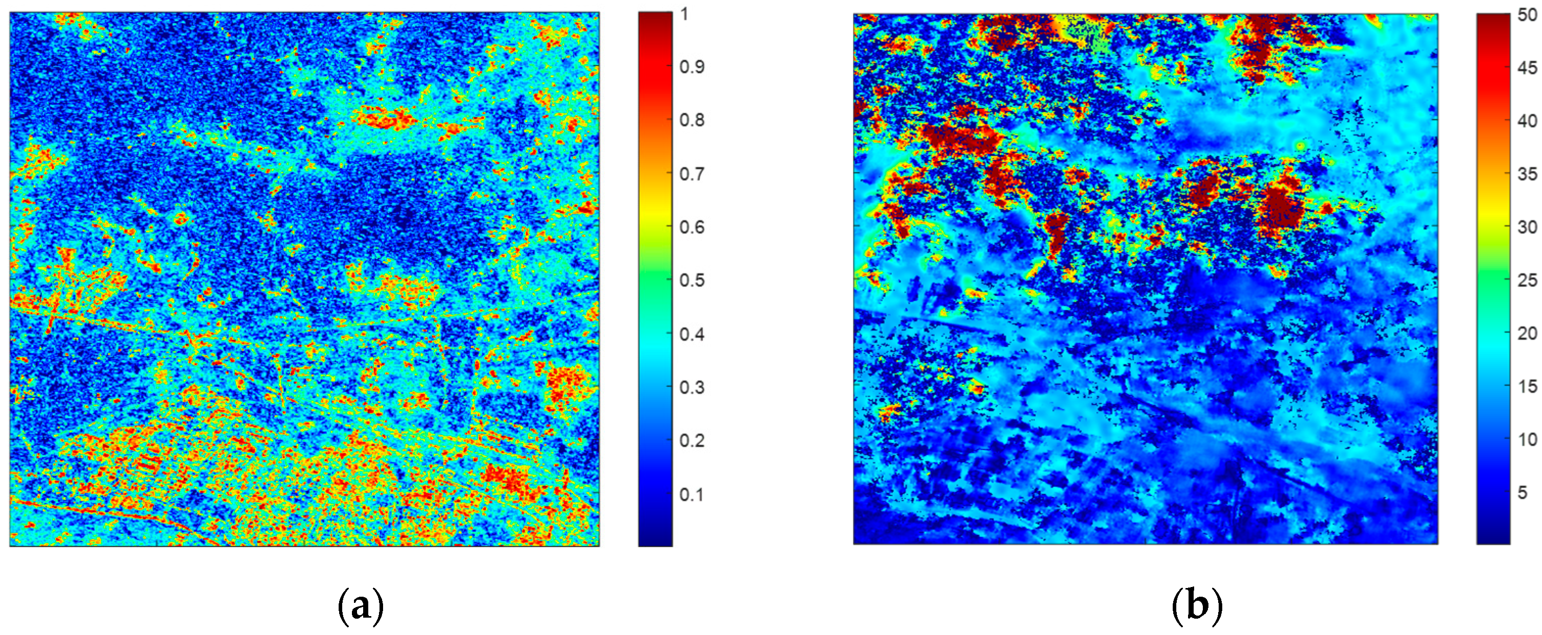
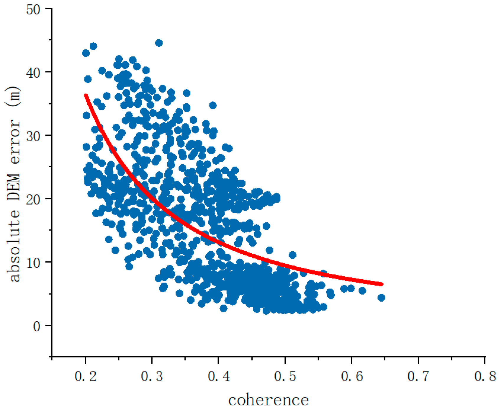
5.1. The Influence of Coherence on the Performance of the Proposed Re-Flattening Method

In this paper, the accuracy of the generated DEM is used to indirectly reflect the performance of the proposed method. GF-3 InSAR data located in Ningbo City was taken as an example for analysis and experiment. The coherence image and corresponding absolute DEM error image in one local area of Ningbo City are enlarged as shown in Figure 20, and they are displayed to show the relationship between the coherence and the accuracy of generated DEM. As can be seen from Figure 20, areas with high coherence which are at the bottom of the image have the smallest absolute DEM error; areas with middle coherence which are in the upper right corner of the image have the middle absolute DEM error; the remaining area with the least coherence has the largest absolute DEM error.

In addition, 1000 points are randomly selected from the image to show the relationship between the coherence and the absolute DEM error, and the results are shown in Figure 21. The coherence is the mean value in a 10 × 10 window centered on each point, and the absolute DEM error is also processed in the same way. As can be seen from Figure 21, the absolute DEM error decreases with the increase in coherence.

The above two experimental results seem to indirectly reflect that the performance of the proposed re-flattening method will be affected by the coherence. However, further analysis is needed to draw conclusions.

The coherence condition of the proposed method and the impact of coherence on the interferometric phase are combined for analysis. When the majority of pixels in the image do not meet the coherence condition, the residual phase fitting and local phase alignment will be seriously affected, and the performance of the proposed method will be greatly reduced. In addition, the interferometric phase at this time is seriously affected by decoherence, which cannot correctly reflect the geometry between the target and antennas. In such a case, the above two points lead to poor DEM accuracy. When most pixels in the image can satisfy the coherence condition, the adaptively adjusted window can remove residual fringes and maintain phase continuity, and the optimal performance of the proposed method can be exerted, as shown in the results in the regions with high coherence in Figure 20. At this time, there are still differences in the DEM errors in different regions, and the value of the DEM error corresponds to the coherence, as shown in Figure 20 and Figure 21. The accuracy of the DEM is mainly affected by the quality of the interferometric phase itself.

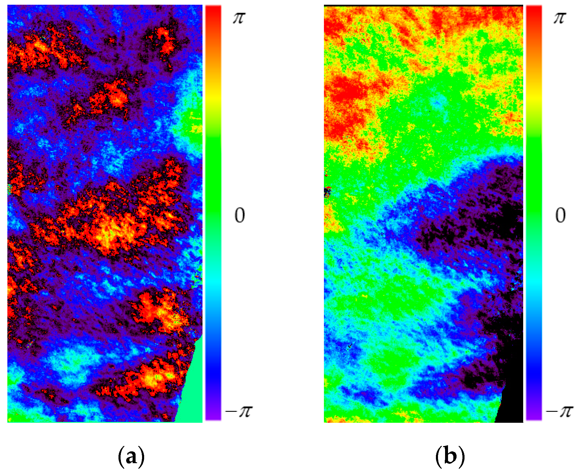
5.2. Comparison with the Result Based on TerraSAR-X Data with Similar Conditions

The accuracy of the DEM obtained by InSAR technology is usually related to the coherence and ambiguity height of InSAR data. As is known to all, when the coherence is higher and the ambiguity height is smaller, the accuracy of the generated DEM will be higher. Regrettably, the InSAR data we have is not very well-conditioned for its low coherence and slightly large ambiguity height. Therefore, the accuracy of the generated DEMs is not very high. However, combined with the data condition of coherence and ambiguity height, the accuracy of the generated DEMs based on the proposed method is reasonable and acceptable.

To confirm the above conclusion, a set of TerraSAR-X InSAR data with high image quality and small baseline error was used for comparison. The generated DEM based on TerraSAR-X is considered reliable and is used as the reference. The same interferometric processing and the proposed re-flattening are carried out for TerraSAR-X InSAR data. The average coherence of the TerraSAR-X data is 0.47, and the ambiguity height is 48.88 m. The comparison of the generated DEMs based on GF-3 InSAR data (Ningbo) and TerraSAR-X InSAR data is shown in Table 3. The MAE of the obtained DEM based on TerraSAR-X data is 11.22 m, and the RMSE is 13.35 m. As can be seen from

Table 4. DEM comparison between GF-3 data (Ningbo) and TerraSAR-X data.

Data\Indicator	Average Coherence	Ambiguity Height (m)	MAE (m)	RMSE (m)
GF-3 InSAR data in Ningbo	0.35	31.05	9.84	15.17
TerraSAR-X InSAR data	0.47	48.88	11.22	13.35

, the coherence and ambiguity height of the TerraSAR-X data are similar to those of the GaoFen-3 InSAR data located in Ningbo, and the DEM accuracy of the two sets of data is also similar, which indicates that the accuracy of the generated DEMs in this paper is reasonable.

More importantly, the reconstructed DEMs are given to obtain a quantitative comparison of these re-flattening methods, and the comparison of the DEMs based on these re-flattening methods should be the focus. The results in Section 4.2 and Section 4.3 have all confirmed that compared with the re-flattening method based on the whole image processing (represented by the polynomial refinement method and the baseline correction-based re-flattening method) and the local frequency estimation and manually designed windows-based method, the method proposed in this paper is more effective in the removal of time-varying and uneven residual fringes.

6. Conclusions

Existing re-flattening methods suffer from the deficiencies of incomplete removal of time-varying and uneven residual fringes. In this paper, an interferogram re-flattening method based on the local residual fringe removal and adaptively adjusted windows was proposed. On the one hand, the time-varying and uneven residual fringes throughout the image can be removed by local re-flattening and re-flattened interferogram splicing. On the other hand, the adaptively adjusted windows are designed to make sure that the residual fringes within the local window can be removed cleanly, and the re-flattened interferograms between adjacent windows can be joined. The proposed re-flattening method was validated using four pairs of InSAR data. The experiments show that compared with the global re-flattening methods and manual window-based local re-flattening method, the proposed method can achieve the full image re-flattening and obtain the DEM reconstruction with higher accuracy. The MAE can be improved by more than 40%, and RMSE can be improved by more than 30%. Both qualitative and quantitative evaluations show that the method proposed in this paper is more effective for the removal of time-varying and non-uniform residual fringes, which is of great significance to improve the utilization and application value of data.

References

1. Short, N.; Brisco, B.; Couture, N.; Pollard, W.; Murnaghan, K.; Budkewitsch, P. A comparison of TerraSAR-X, RADARSAT-2 and ALOS-PALSAR interferometry for monitoring permafrost environments, case study from Herschel Island, Canada. Remote Sens. Environ. 2011, 115, 3491–3506. [Google Scholar] [CrossRef]
2. Prush, V.B.; Lohman, R.B. Time-Varying Elevation Change at the Centralia Coal Mine in Centralia, Washington (USA), Constrained with InSAR, ASTER, and Optical Imagery. IEEE J. Sel. Top. Appl. Earth Obs. Remote Sens. 2015, 8, 919–925. [Google Scholar] [CrossRef]
3. Bayer, B.; Schmidt, D.; Simoni, A. The Influence of External Digital Elevation Models on PS-InSAR and SBAS Results: Implications for the Analysis of Deformation Signals Caused by Slow Moving Landslides in the Northern Apennines (Italy). IEEE Trans. Geosci. Remote Sens. 2017, 55, 2618–2631. [Google Scholar] [CrossRef]
4. Sigmundsson, F.; Hreinsdottir, S.; Hooper, A.; Arnadottir, T.; Pedersen, R.; Roberts, M.J.; Oskarsson, N.; Auriac, A.; Decriem, J.; Einarsson, P.; et al. Intrusion triggering of the 2010 Eyjafjallajokull explosive eruption. Nature 2010, 468, 426–430. [Google Scholar] [CrossRef]
5. Cochrane, T.A.; Egli, M.; Phillips, C.; Acharya, G. Development of a forest road erosion calculation GIS tool for forest road planning and design. In Proceedings of the International Congress on Modelling and Simulation: Land, Water, & Environmental Management: Integrating Systems for Sustainability, Christchurch, New Zealand, 1–5 December 2007. [Google Scholar]
6. Buğday, E. Capabilities of using UAVs in forest road construction activities. Eur. J. For. Eng. 2018, 4, 56–62. [Google Scholar] [CrossRef]
7. Tran, D.; Xu, D.; Dang, V.; Alwah, A.A.Q. Predicting Urban Waterlogging Risks by Regression Models and Internet Open-Data Sources. Water 2020, 12, 879. [Google Scholar] [CrossRef]
8. Bhatt, C.M.; Srinivasa Rao, G. HAND (height above nearest drainage) tool and satellite-based geospatial analysis of Hyderabad (India) urban floods, September 2016. Arab. J. Geosci. 2018, 11, 600. [Google Scholar] [CrossRef]
9. Li, D.; Zhu, X.; Huang, G.; Feng, H.; Zhu, S.; Li, X. A hybrid method for evaluating the resilience of urban road traffic network under flood disaster: An example of Nanjing, China. Environ. Sci. Pollut. Res. 2022, 29, 46306–46324. [Google Scholar] [CrossRef] [PubMed]
10. Mohammadi Samani, K.; Hosseini, S.A.; Lotfian, M.; Najafi, A. Planning road network in mountain forests using GIS and Analytic Hierarchical Process (AHP). Casp. J. Environ. Sci. 2010, 8, 151–162. [Google Scholar]
11. Rouet-Leduc, B.; Jolivet, R.; Dalaison, M.; Johnson, P.A.; Hulbert, C. An identification method of potential landslide zones using InSAR data and landslide susceptibility. Geomat. Nat. Hazards Risk 2023, 14, 2185120. [Google Scholar] [CrossRef]
12. Rouet-Leduc, B.; Jolivet, R.; Dalaison, M.; Johnson, P.A.; Hulbert, C. Autonomous extraction of millimeter-scale deformation in InSAR time series using deep learning. Nat. Commun. 2021, 12, 6480. [Google Scholar] [CrossRef]
13. Anantrasirichai, N.; Biggs, J.; Kelevitz, K.; Sadeghi, Z.; Wright, T.; Thompson, J.; Achim, A.M.; Bull, D. Detecting ground deformation in the built environment using sparse satellite InSAR data with a convolutional neural network. IEEE Trans. Geosci. Remote Sens. 2020, 59, 2940–2950. [Google Scholar] [CrossRef]
14. Small, D.; Werner, C.; Nuesch, D. Base-Line Modeling for ERS-1 SAR Interferometry. In Proceedings of the IGARSS 93, Kogakuin Univ, Tokyo, Japan, 18–21 August 1993. [Google Scholar]
15. Cao, Y.X.; Fan, Z.; Chen, Y. Flat Earth Removal and Baseline Estimation Based on Orbit Parameters Using Radarsat-2 Image. In Proceedings of the IGARSS 2013, Melbourne, Australia, 21–26 July 2013. [Google Scholar]
16. Geudtner, D.; Schwäbisch, M. An Algorithm for Precise Reconstruction of InSAR Imaging Geometry: Application to “Flat-Earth” Phase Removal, Phase-to-Height Conversion and Geocoding of InSAR-Derived DEMs. In Proceedings of the EUSAR ‘96 (1996), Königswinter, Germany, 26–28 March 1996. [Google Scholar]
17. Kimura, H.; Todo, M. Baseline estimation using ground points for interferometric SAR. In Proceedings of the IGARSS 97, Singapore, 3–8 August 1997. [Google Scholar]
18. Chen, X.T.; Zhu, X.F.; Wang, X.H.; Cai, Y. INSAR Flat-Earth Phase Removal Approach Based on DEM to Settlement Area. In Proceedings of the ITM Web of Conferences, Hangzhou, China, 29–31 July 2016. [Google Scholar]
19. Gatelli, F.; Guamieri, A.M.; Parizzi, F.; Pasquali, P.; Prati, C.; Rocca, F. The Wave-Number Shift in SAR Interferometry. IEEE Trans. Geosci. Remote Sens. 1994, 32, 855–865. [Google Scholar] [CrossRef]
20. Moreira, J.; Schwabisch, M.; Fornaro, G. X-SAR Interferometry—First Results. IEEE Trans. Geosci. Remote Sens. 1995, 33, 950–956. [Google Scholar] [CrossRef]
21. Lanari, R.; Fornaro, G.; Riccio, D.; Migliaccio, M.; Papathanassiou, K.P.; Moreira, J.R.; Schwabisch, M.; Dutra, L.; Puglisi, G.; Franceschetti, G.; et al. Generation of digital elevation models by using SIR-C/X-SAR multifrequency two-pass interferometry: The Etna case study. IEEE Trans. Geosci. Remote Sens. 1996, 34, 1097–1114. [Google Scholar] [CrossRef]
22. Xiang, Z.; Wang, K.Z.; Liu, X.Z. A Model-Spectrum-Based Flattening Algorithm for Airborne Single-Pass SAR Interferometry. IEEE Geosci. Remote Sens. Lett. 2009, 6, 307–311. [Google Scholar] [CrossRef]
23. Peng, S.R.; He, K.X.; Wang, Y.N. A High Accurate Approach for InSAR Flat Earth Effect Removal. In Proceedings of the 2009 International Conference on Measuring Technology and Mechatronics Automation, Zhangjiajie, China, 11–12 April 2009. [Google Scholar]
24. Qu, C.Y.; Shan, X.J.; Zhang, G.H.; Song, X.G.; Zhang, G.F.; Liu, Y.H.; Guo, L.M. Influence of interferometric baseline on measurements of seismic deformation: A case study on the 1997 mani, tibet m 7.7 earthquake. Seismol. Geol. 2012, 34, 672–683. [Google Scholar]
25. Xiang, Z.; Wang, K.Z.; Liu, X.Z.; Yu, W.X. Analysis of the InSAR Flattening Errors and Their Influence on DEM Reconstruction. In Proceedings of the 2009 IEEE Radar Conference, Pasadena, CA, USA, 4–8 May 2009. [Google Scholar]
26. Massonnet, D.; Feigl, K.L. Radar interferometry and its application to changes in the Earth’s surface. Rev. Geophys. 1998, 36, 441–500. [Google Scholar] [CrossRef]
27. Shirzaei, M.; Walter, T.R. Estimating the effect of satellite orbital error using wavelet-based robust regression applied to InSAR deformation data. IEEE Trans. Geosci. Remote Sens. 2011, 49, 4600–4605. [Google Scholar] [CrossRef]
28. Liu, Z.; Jung, H.-S.; Lu, Z. Joint correction of ionosphere noise and orbital error in L-band SAR interferometry of interseismic deformation in southern California. IEEE Trans. Geosci. Remote Sens. 2013, 52, 3421–3427. [Google Scholar] [CrossRef]
29. Du, Y.; Fu, H.; Liu, L.; Feng, G.; Peng, X.; Wen, D. Orbit error removal in InSAR/MTInSAR with a patch-based polynomial model. Int. J. Appl. Earth Obs. Geoinf. 2021, 102, 102438. [Google Scholar] [CrossRef]
30. Sahraoui, O.H.; Hassaine, B.; Serief, C.; Hasni, K. Radar interferometry with Sarscape software. In Proceedings of the Shaping Change XXIII FIG Congress, Munich, Germany, 8–13 October 2006. [Google Scholar]
31. Polcari, M.; Albano, M.; Montuori, A. InSAR Monitoring of Italian Coastline Revealing Natural and Anthropogenic Ground Deformation Phenomena and Future Perspectives. Sustainability 2018, 10, 3152. [Google Scholar] [CrossRef]
32. Sataer, G.; Sultan, M.; Emil, M.K. Remote Sensing Application for Landslide Detection, Monitoring along Eastern Lake Michigan (Miami Park, MI). Remote Sens. 2022, 14, 3474. [Google Scholar] [CrossRef]
33. Xiao, B.; Zhao, J.S.; Li, D.S. The Monitoring and Analysis of Land Subsidence in Kunming (China) Supported by Time Series InSAR. Sustainability 2022, 14, 12387. [Google Scholar] [CrossRef]
34. Gaber, A.; Darwish, N.; Koch, M. Minimizing the Residual Topography Effect on Interferograms to Improve DInSAR Results: Estimating Land Subsidence in Port-Said City, Egypt. Remote Sens. 2017, 9, 752. [Google Scholar] [CrossRef]
35. Parihar, N.; Nathawat, M.S.; Das, A.K.; Mohan, S. Accuracy assessment of DEMs derived from multi-frequency SAR images. In Proceedings of the 3rd APSAR, Seoul, Republic of Korea, 26–30 September 2011. [Google Scholar]
36. Xu, B.; Li, Z.; Zhu, Y.; Shi, J.; Feng, G. SAR Interferometric Baseline Refinement Based on Flat-Earth Phase without a Ground Control Point. Remote Sens. 2020, 12, 233. [Google Scholar] [CrossRef]
37. Wang, H.Q.; Zhou, Y.S.; Fu, H.Q. Parameterized Modeling and Calibration for Orbital Error in TanDEM-X Bistatic SAR Interferometry over Complex Terrain Areas. Remote Sens. 2021, 13, 5124. [Google Scholar] [CrossRef]
38. Lin, C.-y.; Chen, L.; Ge, S.-q. Research on method of flat earth effect removal based on refined local fringe frequency. In Proceedings of the IET International Radar Conference 2013, Xi’an, China, 14–16 April 2013. [Google Scholar]
39. Ai, B.; Liu, K.; Li, X.; Li, D.H. Flat-earth phase removal algorithm improved with frequency information of interferogram. In Proceedings of the Geoinformatics 2008 and Joint Conference on GIS and Built Environment: Geo-Simulation and Virtual GIS Environments, Guangzhou, China, 28–29 June 2008. [Google Scholar]
40. Yubin, Z.; Jie, Z.; Junmin, M.; Chenqing, F. An improved frequency shift method for ATI-SAR flat earth phase removal. Acta Oceanol. Sin. 2019, 38, 94–100. [Google Scholar] [CrossRef]
41. Liu, G.; Hanssen, R.F.; Guo, H.; Yue, H.; Perski, Z. Nonlinear model for InSAR baseline error. IEEE Trans. Geosci. Remote Sens. 2016, 54, 5341–5351. [Google Scholar] [CrossRef]
42. Lu, H.; Suo, Z.; Li, Z.; Xie, J.; Zhao, J.; Zhang, Q. InSAR Baseline Estimation for Gaofen-3 Real-Time DEM Generation. Sensors 2018, 18, 2152. [Google Scholar] [CrossRef]
43. Goldstein, R.M.; Werner, C.L. Radar interferogram filtering for geophysical applications. Geophys. Res. Lett. 1998, 25, 4035–4038. [Google Scholar] [CrossRef]
44. Baran, I.; Stewart, M.P.; Kampes, B.M.; Perski, Z.; Lilly, P. A modification to the Goldstein radar interferogram filter. IEEE Trans. Geosci. Remote Sens. 2003, 41, 2114–2118. [Google Scholar] [CrossRef]
45. Costantini, M. A novel phase unwrapping method based on network programming. IEEE Trans. Geosci. Remote Sens. 1998, 36, 813–821. [Google Scholar] [CrossRef]
46. Ullah, Z.; Usman, M.; Jeon, M.; Gwak, J. Cascade multiscale residual attention cnns with adaptive roi for automatic brain tumor segmentation. Inf. Sci. 2022, 608, 1541–1556. [Google Scholar] [CrossRef]
47. Ullah, Z.; Farooq, M.U.; Lee, S.H.; An, D. A hybrid image enhancement based brain MRI images classification technique. Med. Hypotheses 2020, 143, 109922. [Google Scholar] [CrossRef] [PubMed]
Figure 1. Examples of the flattened interferograms using the orbit-based flattening method. (a) Flattened interferograms in Tokyo Bay area based on GaoFen-3 FSII data; (b) Flattened interferograms in Ningbo City area based on GaoFen-3 FSI data.
Remotesensing 15 02214 g001
Figure 2. Flowchart of the proposed method.
Remotesensing 15 02214 g002
Figure 3. Mechanism of adaptive adjustment for re-flattening windows.
Remotesensing 15 02214 g003
Figure 4. The situations of the residual fringes not being removed completely and the corresponding solution. (a) Re-flattened interferogram with residual fringes due to a small window; (b) Re-flattened interferogram without residual fringes after adaptive window size adjustment; (c) Re-flattened interferogram with residual fringes due to the improper position; (d) Re-flattened interferogram without residual fringes after adaptive position adjustment.
Remotesensing 15 02214 g004
Figure 5. Schematic diagram of the re-flattened interferogram. (a) re-flattened interferogram within one column of windows; (b) re-flattened interferogram within several columns of windows. The blue arrow indicates the order of the re-flattening process.
Remotesensing 15 02214 g005
Figure 6. SAR intensity images and corresponding optical images of the four pairs of InSAR data. (a) SAR intensity image of the GF-3 InSAR data located in Ningbo City; (b) Optical image of the GF-3 InSAR data located in Ningbo City; (c) SAR intensity image of the GF-3 InSAR data located in Yutian County; (d) Optical image of the GF-3 InSAR data located in Yutian County; (e) SAR intensity image of the GF-3 InSAR data located in Xi’an City; (f) Optical image of the GF-3 InSAR data located in Xi’an City; (g) SAR intensity image of the Sentinel-1A InSAR data located in Yancheng City; (h) Optical image of the Sentinel-1A InSAR data located in Yancheng City.
Remotesensing 15 02214 g006aRemotesensing 15 02214 g006b
Figure 7. Interferogram and coherence of the InSAR data located in Ningbo. (a) Interferogram; (b) The enlarged image of the red rectangular window in (a); (c) Coherence; (d) The histogram of the coherence.
Remotesensing 15 02214 g007
Figure 8. Flattened interferogram.
Remotesensing 15 02214 g008
Figure 9. The re-flattened interferograms of local windows and phase alignment between adjacent windows. (a) The re-flattened and aligned interferogram; (b) The interferogram after re-flattening and phase alignment of the next window, based on (a); (c) The enlarged image of the red rectangular window in (b).
Remotesensing 15 02214 g009
Figure 10. Re-flattened interferograms based on the proposed method, GPR method, SBDR method and LFE-MW method. (a) The re-flattened interferogram based on the proposed re-flattening method in this paper; (b) The enlarged image of the red rectangular window in (a); (c) The re-flattened interferogram based on the GPR method; (d) The enlarged image of the red rectangular window in (c); (e) The re-flattened interferogram based on the SBDR method; (f) The enlarged image of the red rectangular window in (e); (g) The re-flattened interferogram based on the LFE-MW method; (h) The enlarged image of the red rectangular window in (g).
Remotesensing 15 02214 g010aRemotesensing 15 02214 g010b
Figure 11. Re-flattened interferograms of the InSAR data located in Yutian County. (a) Re-flattened interferogram based on the proposed re-flattening method; (b) Re-flattened interferogram based on the GPR method; (c) Re-flattened interferogram based on the SBDR method; (d) Re-flattened interferogram based on the LFE-MW method.
Remotesensing 15 02214 g011
Figure 12. Re-flattened interferograms of the InSAR data located in Xi’an City. (a) Re-flattened interferogram based on the proposed re-flattening method; (b) Re-flattened interferogram based on the GPR method; (c) Re-flattened interferogram based on the SBDR method; (d) Re-flattened interferogram based on the LFE-MW method.
Remotesensing 15 02214 g012
Figure 13. Re-flattened interferograms of the Sentinel-1A InSAR data located in Yancheng City. (a) Re-flattened interferogram based on the proposed re-flattening method; (b) Re-flattened interferogram based on the GPR method; (c) Re-flattened interferogram based on the SBDR method; (d) Re-flattened interferogram based on the LFE-MW method.
Remotesensing 15 02214 g013aRemotesensing 15 02214 g013b
Figure 14. DEMs (in meters) in Ningbo City based on different re-flattened interferograms. (a) DEM based on the proposed re-flattening method; (b) DEM based on the GPR method; (c) DEM based on the SBDR method; (d) DEM based on the LFE-MW method.
Remotesensing 15 02214 g014aRemotesensing 15 02214 g014b
Figure 15. DEMs (in meters) in Yutian County based on different re-flattened interferograms. (a) DEM based on the proposed re-flattening method; (b) DEM based on the GPR method; (c) DEM based on the SBDR method; (d) DEM based on the LFE-MW method.
Remotesensing 15 02214 g015
Figure 16. DEMs (in meters) in Xi’an City based on different re-flattened interferograms. (a) DEM based on the proposed re-flattening method; (b) DEM based on the GPR method; (c) DEM based on the SBDR method; (d) DEM based on the LFE-MW method.
Remotesensing 15 02214 g016aRemotesensing 15 02214 g016b
Figure 17. DEMs (in meters) in Yancheng City based on different re-flattened interferograms. (a) DEM based on the proposed re-flattening method; (b) DEM based on the GPR method; (c) DEM based on the SBDR method; (d) DEM based on the LFE-MW method.
Remotesensing 15 02214 g017
Figure 18. The lines of relative evaluation indicators Δ M A E and Δ R M S E . (a) The line of Δ M A E ; (b) the line of Δ R M S E .
Remotesensing 15 02214 g018
Figure 19. Building height estimation based on the re-flattened interferogram which uses the proposed method. (a) Optical image, (b) Re-flattened interferogram and (c) Height estimation of the selected buildings in area1; (d) Optical image, (e) Re-flattened interferogram and (f) Height estimation of the selected buildings in area2; (g) Optical image, (h) Re-flattened interferogram and (i) Height estimation of the selected buildings in area3; (j) Optical image, (k) Re-flattened interferogram and (l) Height estimation of the selected buildings in area4.
Remotesensing 15 02214 g019
Figure 20. Enlarged coherence image and absolute DEM error image in the local area of Ningbo City. (a) The coherence image of the local area in Ningbo City; (b) the corresponding absolute DEM error to (a).
Remotesensing 15 02214 g020
Figure 21. The relationship between the coherence and the absolute DEM error.
Remotesensing 15 02214 g021