Radiometric Terrain Correction Method Based on RPC Model for Polarimetric SAR Data

Abstract

Radiometric terrain correction (RTC) is an important preprocessing step for synthetic aperture radar (SAR) data application in mountainous areas. At present, the RTC processing of SAR depends on the Range Doppler (RD) positioning model. However, the solution of this model has a high threshold for ordinary remote sensing technicians. To solve this problem, we propose an RTC method based on the rational polynomial coefficient (RPC) model, which is widely used in optical remote sensing and is simpler and more practical than the RD model. China’s GF-3 polarimetric SAR data were used to verify the proposed method. The experimental results showed that the RTC method based on RPC is effective and can achieve better correction effects on the premise of reducing the complexity of the algorithm. The correction effect based on the RPC model can be similar to that based on the RD model. The proposed approach can realize the correction of 4~5 dB terrain radiation distortion to a 0.5 dB level.

1. Introduction

Synthetic aperture radar (SAR) is a kind of sensor that can realize all-day and all-weather imaging. The unique advantages of the SAR satellite make it an indispensable tool for observation in the field of earth observation. However, owing to the characteristics of the side-looking illumination used in SAR sensors, terrain undulations seriously affect the radiometric quality of SAR images [1]. Therefore, radiometric terrain correction (RTC) is an essential processing step for the application of SAR data in mountainous areas [2]. In general, standard SAR products do not include data after RTC processing. For users of SAR data, especially users of polarization SAR data, the object of RTC is a polarization scattering matrix containing complex numbers. As a result, the users need to implement preprocessing steps containing geocoding of terrain correction (GTC) and RTC based on single-look complex (SLC)-level SAR images. However, these processing steps are not easy and, to some extent, hinder the wide application of SAR data.

In fact, the RTC method itself is not too difficult for general users. After years of research, researchers have developed a series of systems and mature methods for the RTC of SAR data [3,4,5,6,7]. It is mainly divided into three aspects: the polarization orientation angle (POA) correction of the polarization state, the effective scattering area (ESA) correction of the number of scatterers, and the angle variation effect (AVE) of the scattering mechanism. It should be noted that the above RTC method needs to obtain local imaging geometric information (local incidence angle, projection angle, etc.) on the basis of digital elevation model (DEM) data. At present, the conventional method is to construct the Range Doppler (RD) position model to realize the geocoding of the SAR image and obtain the corresponding relationship between the geographic location of each pixel of the SAR image and the imaging position of the SAR sensor, thereby calculating the local geometry angles of SAR imaging [2]. This method first needs to master the solution of the RD positioning model, which usually requires the design of a complicated iterative algorithm and requires more SAR imaging parameters. It is difficult for general users to program and solve the RD positioning model by themselves in the process of applying SAR data. As for business software, such as GAMMA (version: 2012) [8], local imaging geometric information is provided by the GTC module, but it is expensive and not all users can afford it. For free SAR processing software, all the imaging geometric information is usually not provided. For example, SNAP software only provides local incident angle information [9].

In summary, the special data formats, complex processing algorithms, and expensive business software required for SAR data have hindered its widespread application to a certain extent. Therefore, for ordinary users of SAR data, there is an urgent need to develop a method of implementing RTC with relatively low technical thresholds. Fortunately, some of China’s SAR satellites, such as GaoFen-3 (GF-3) and LuTan-1 (LT-1), allow this idea to be realized. Take GF-3 as an example: the SAR data of the GF-3 satellite provide rational polynomial coefficient (RPC) files (*.rpc), which contain the mapping relationship between the radar range space and the geographical space [10]. Therefore, for the GTC and RTC processing of SAR data, the RPC model can replace the RD positioning model. In fact, as early as 2008, G. Zhang et al. [11] introduced the RPC model, which is commonly used in optical remote sensing and the geometric processing of SAR data. Compared to the RD positioning model, this model is more familiar and easier for ordinary remote sensing technicians. The advantage is that SAR users can implement the geocoding processing of different SAR satellite data based on the RPC model using common RPC files and general algorithms/software. Of course, at present, only a small number of SAR satellites provide RPC files. In terms of RPC-based SAR data preprocessing, many studies [12,13,14,15,16] have proposed a method of implementing the GTC of SAR data based on the RPC model. However, no one has explained how to implement RTC processing based on the RPC model. This is a technical gap that needs to be supplemented.

In this study, we propose the RTC approach of polarimetric SAR (PolSAR) based on the RPC model, which takes advantage of the RPC general geometry model. It does not need to implement the solution of the RD position model, and only needs a small number of SAR imaging parameters to complete the RTC of PolSAR data. The article is structured as follows. The study area, the experimental data, and the method used to calculate the local imaging geometric information based on the RPC model and the RTC method are outlined in Section 2. In Section 3, the proposed method is demonstrated using polarization SAR data of the GF-3 satellite. Finally, the discussion and conclusion are presented in Section 4 and Section 5, respectively.

2. Materials and Methods

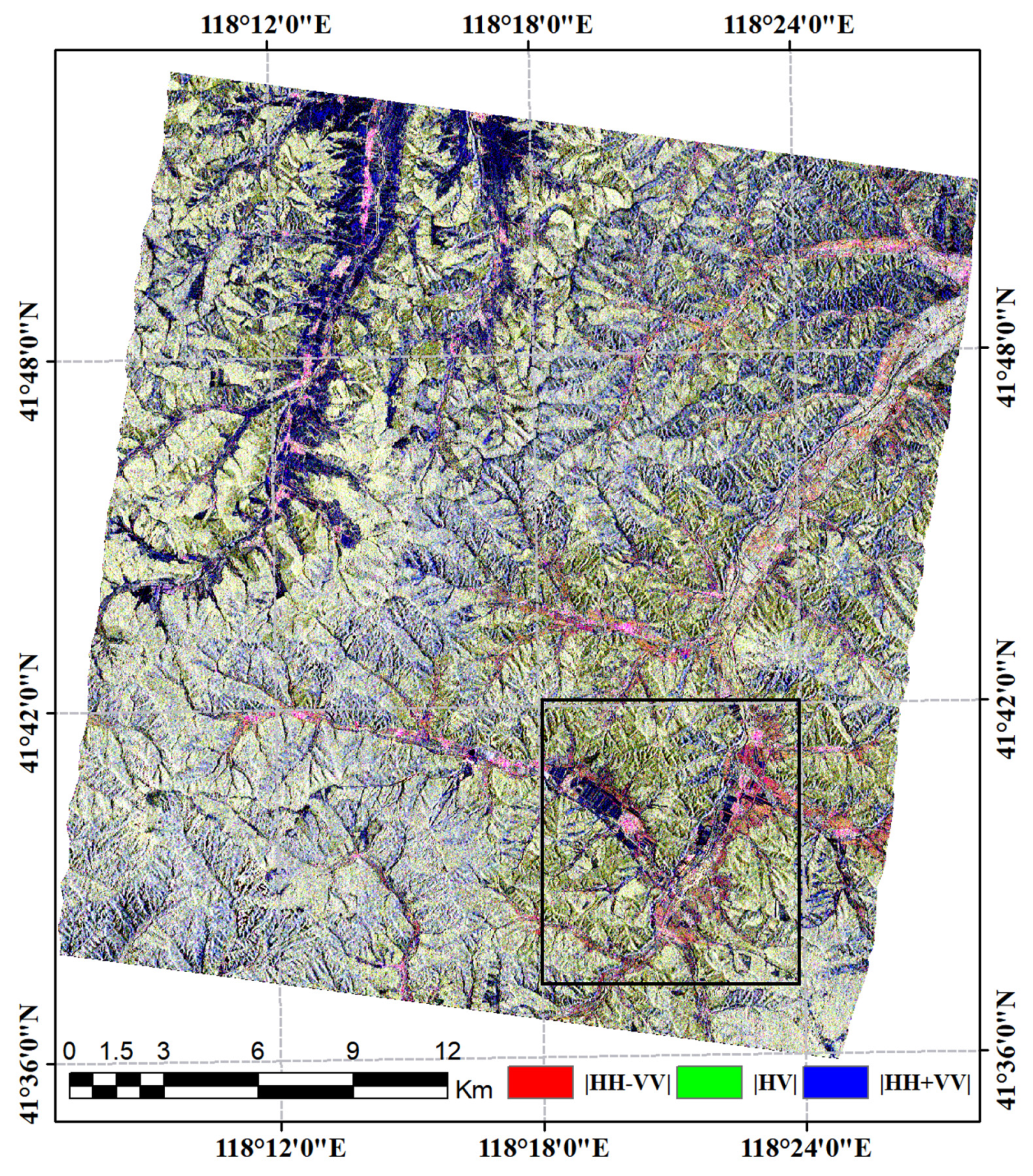
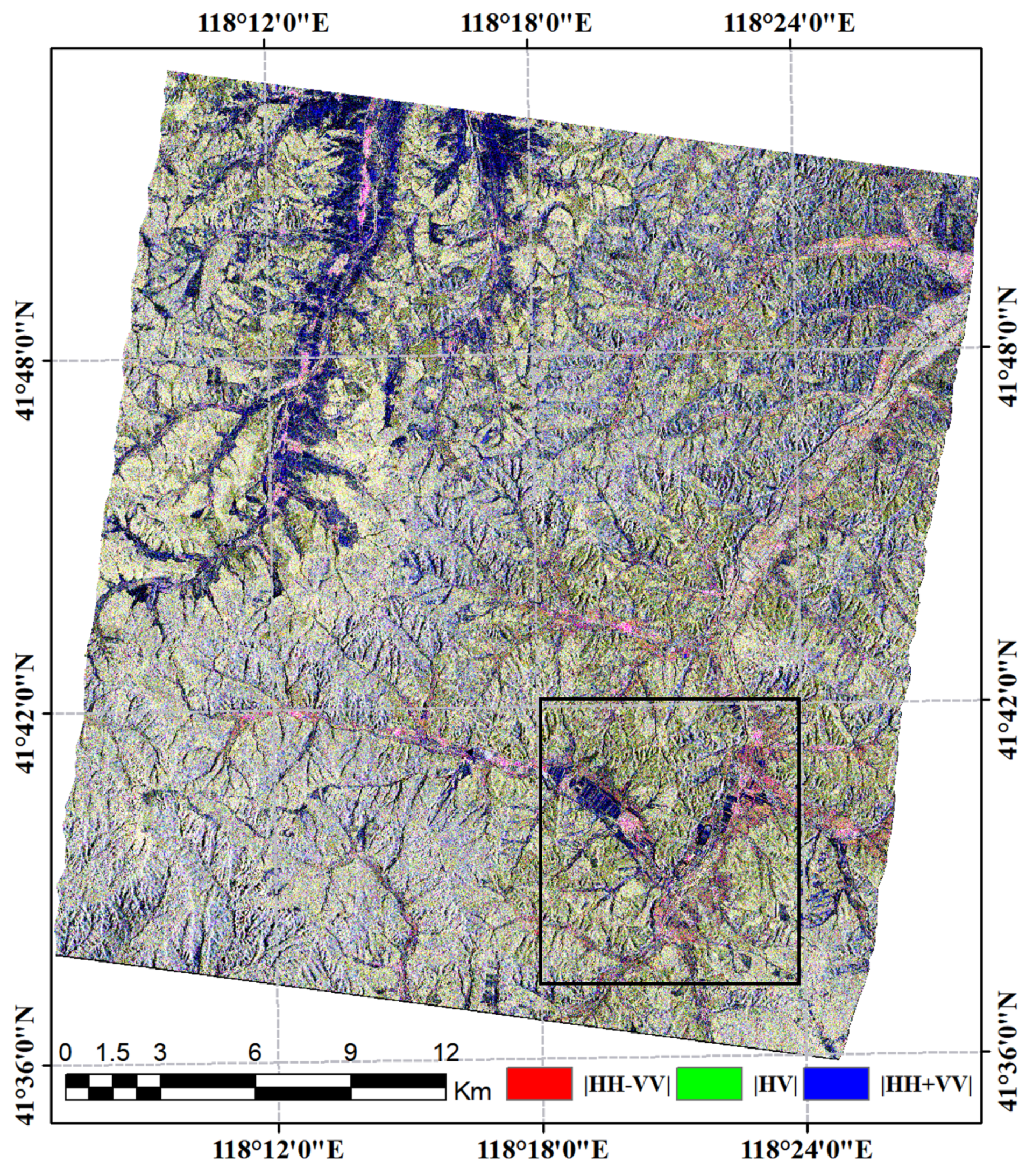
2.1. Test Site and Data

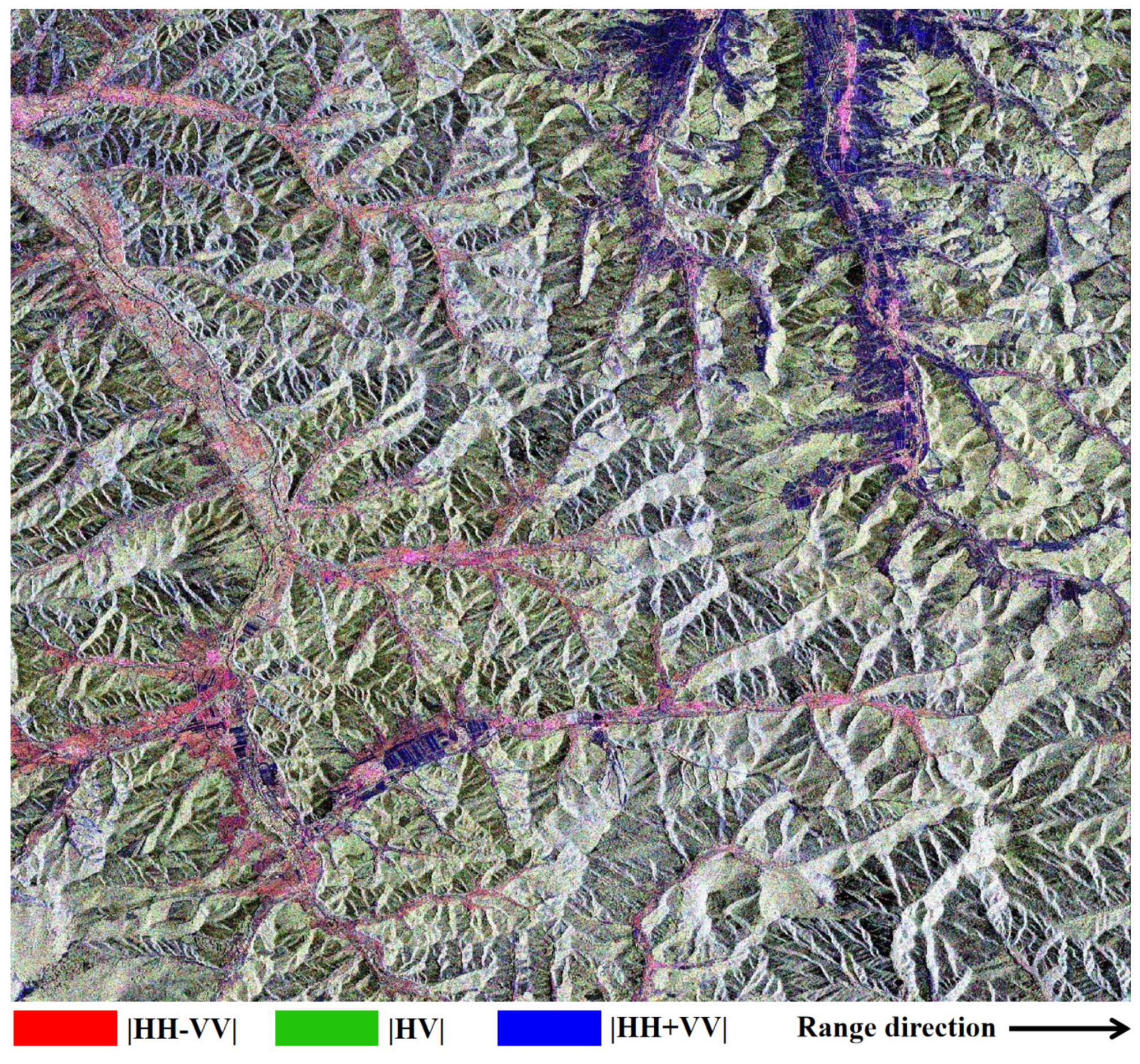
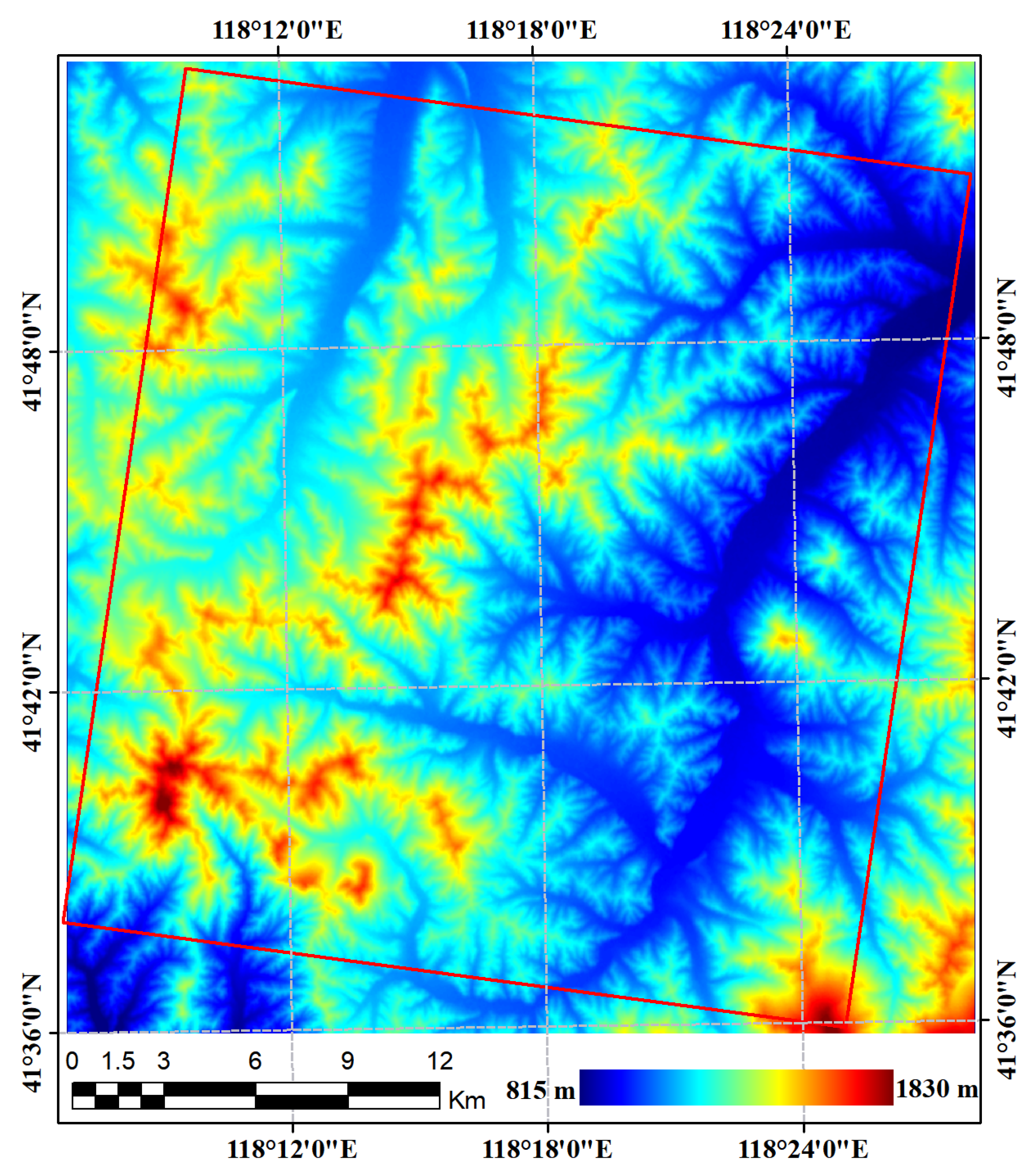
2.1.1. Test Site

As shown in Figure 1, the test site was located in Chifeng, Inner Mongolia, China [118.25°E, 41.73°N], with altitudes ranging from 815 to 1830 m. Mountains are the main geographic component of this region, and the slopes are relatively short and steep. The area is mainly covered by forests, with a small number of buildings and farmland. The main tree species present are Chinese pine (Pinus tabulaeformis Carr) and Larix Principis (Larix principis-rupprechtii May).

2.1.2. PolSAR and Auxiliary Data

In this study, one scene of GF-3 PolSAR data was acquired over the test site on 25 September 2019. The observation model used was quad-polarization stripe 1 (QPSI). The SLC pixel spacing of the azimuth and range direction were 5.0 and 4.5 m, respectively. The coverage of the data (Figure 1, red rectangle) was 25 km wide (east-west) and 30 km long (north-south). Figure 2 shows the Pauli RGB display of the PolSAR data (multi-looked, window: 2 × 3). It shows a very obvious terrain effect. In the range direction, the slopes facing the SAR sensor (front slopes) are short and bright compared to the back slopes.

In addition, DEM data are the necessary auxiliary data needed for the RTC. Here, 1-arcsec SRTM DEM was used for GTC and RTC. Taking into account the SLC resolution of GF-3 PolSAR data, the original DEM data, with a resolution of about 30 m, were resampled to a 15 m resolution, as shown in Figure 3.

2.2. The RTC Method Based on RPC Model

2.2.1. RPC Model

The RPC model is a rational polynomial model containing 90 parameters [11]. The basic forms are shown in Equation (1):

$$X=\frac{N_s\left(P,L,H\right)}{D_s\left(P,L,H\right)},Y=\frac{N_l\left(P,L,H\right)}{D_l\left(P,L,H\right)}$$

(1)

where (X, Y) are the standardized image coordinates of the radar range space, corresponding to the range direction and azimuth direction. Additionally, (P, L, H) are the standardized image coordinates of the geographical space, corresponding to the latitude, longitude, and altitude. The standardized formulas are shown in Equation (2):

$$\begin{array}{l}X=\frac{s-s_{off}}{s_{scale}},Y=\frac{l-l_{off}}{l_{scale}}\\ P=\frac{D_{lat}-D_{lat\_off}}{D_{lat\_scale}},L=\frac{D_{lon}-D_{lon\_off}}{D_{lon\_scale}},H=\frac{D_{hei}-D_{hei\_off}}{D_{hei\_scale}}\end{array}$$

(2)

where (s, l) are the actual (un-standardized) image coordinates of the radar range space, and (D_lat, D_lon, D_hei) are the actual image coordinates of the geographical space. D_{lat_off}, D_{lat_scale}, D_{lon_off}, D_{lon_scale}, D_{hgt_off}, and D_{hgt_scale} are the standardized parameters of the geographic coordinates and s_off, s_scale, l_off, and l_scale are the standardized parameters of the SLC image pixel coordinates. The above 10 standardized parameters are part of the 90 parameters used in the RPC model, and the other 80 parameters constitute four polynomials, which are N_l(), D_l(), N_s(), and D_s() in Equation (1). For example, the form of the polynomial N_l() is as follows:

$$\begin{array}{l}{N}_l\left(P,L,H\right)=a_1+a_{2}L+a_{3}P+a_{4}H+a_{5}LP+a_{6}LH+a_{7}PH+a_8{L}^2+a_9{P}^2\\ \begin{array}{ccccc}& & & & \end{array}+a_{10}{H}^2+a_{11}PLH+a_{12}{L}^3+a_{13}L{P}^2+a_{14}L{H}^2+a_{15}{L}^{2}P+a_{16}{P}^3\\ \begin{array}{ccccc}& & & & \end{array}+a_{17}P{H}^2+a_{18}{L}^{2}H+a_{19}{P}^{2}H+a_{20}{H}^3\end{array}$$

(3)

where a_i are the 20 polynomial coefficients. D_l(), N_s() and D_s() are polynomials of the same form.

The RPC file (*.rpc) provided by the GF-3 satellite SAR data contains the above 90 model parameters. Therefore, the above RPC model can be used to establish the relationship between the radar range space (s, l) and geographical space (D_lat, D_lon, D_hei).

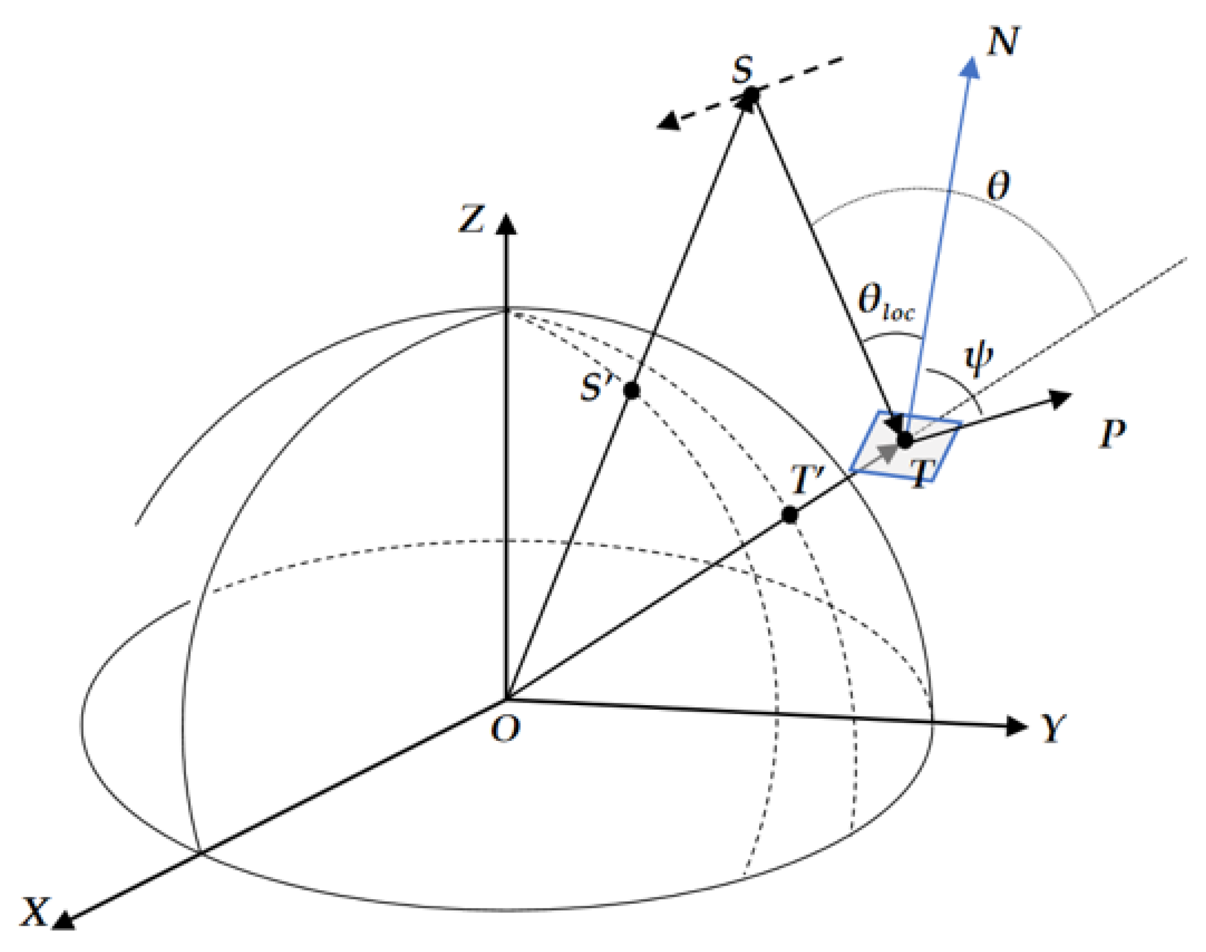
2.2.2. Calculation of Local Geometry Angles Based on RPC Model

Local imaging geometric information is the basis of RTC processing. As shown in Figure 4, it is the local geometric relationship of SAR imaging under an earth-centered rotating (ECR) coordinate system. O is the center of the earth; T is a target point with a certain elevation corresponding to a pixel of the SAR image; S represents the position of the SAR sensor, that is, the imaging location of the sensor for target T; S′ and T′ are the projection point of S and T on the surface of the earth ellipsoid. TN is the normal vector of the local surface around target T. The vector TP is perpendicular to the incidence plane. The projection angle (ψ), local incidence angle (θ_loc), and incidence angle of a horizontal surface (θ) are the local imaging angle information required by the subsequent RTC process.

The entire computing process needs to be based on the DEM data and the imaging parameters in the metadata files (*.meta.xml) of SAR data. The globally shared DEM data, such as ASTER DEM, SRTM DEM, and ALOS 3D DSM, are the data sources that can be used. In addition, we summarized the imaging parameters required in metadata files, as shown in

Table 1. The imaging parameters in GF-3 metadata required for calculation of local geometry angles based on RPC model.

Label in Metadata	Definition	Parameters
<corner>/<topLeft>  …	The longitude and latitude coordinates of the four corner points of the SAR image coverage.	Dlat, Dlon
<imagingTime>/<start>	The starting imaging time of SAR sensor.	T0
<eqvPRF>	Pulse repetition frequency.	PRF
<GPSParam>/<TimeStamp>  /<xPosition>  /<yPosition>  /<zPosition>	Satellite orbit information:  imaging time;  position vectors at different times.	Ti  xPi  yPi  zPi

. The calculation of local geometry angles based on the RPC model can be divided into four steps.

• Preparation of DEM data.

First, according to the longitude and latitude coordinates of the four corners of the SAR image in the metadata (“<corner>”), the coverage of the DEM data can be determined. Then, the DEM data in this range can be extracted to build the DEM grid. For the method proposed in this paper, the DEM grid data should be the geodetic coordinates under the WGS-84 coordinate system, recorded as (D_lat, D_lon, D_hei). In addition, this step also needs to consider the spatial resolution difference between SAR data and DEM data. If necessary, DEM data should be resampled.

• Determine the SAR sensor imaging position (S) corresponding to the target (T).

Based on the RPC model, the image coordinates of the radar range space (s, l) corresponding to each pixel of DEM (D_lat, D_lon, D_hei) can be calculated. Then, the imaging time of each SAR image pixel (T) can be obtained according to the starting imaging time “<imagingTime>/<start>”, T₀) and pulse repetition frequency (“<eqvPRF>”, PRF) parameters of the SAR image:

$$T=T_0+l\cdot N_a/PRF$$

(4)

where l represents the azimuth coordinates, counting from 0, and the reciprocal of PRF is equal to the imaging time of each row of SAR data, and N_a is the number of multi-looks in the azimuth direction. For SLC products, N_a is equal to 1. Next, the SAR sensor imaging position (xP, yP, zP) corresponding to the target pixel (D_lat, D_lon, D_hei) can be determined based on the sequence information of the time (T_i) and the location of the SAR sensor (xP_i, yP_i, zP_i) provided in the metadata (“<GPSParam>”). Additionally, the interpolation processing may be necessary. For example, the metadata of SAR data of GF-3 provides the vector of imaging time and position at an interval of 1 s. Therefore, SAR users can fit these discrete points to obtain the imaging position corresponding to any imaging time. In addition, it should be noted that the sensor location provided in the SAR metadata file is the ECR coordinate.

• Convert the longitude and latitude coordinates of DEM pixels to ECR coordinates.

In order to facilitate the subsequent calculation of local imaging geometric angle, the geodetic coordinates of the DEM grid also need to be converted to the ECR coordinate system. The conversion formula from WGS-84 geodetic coordinates (D_lat, D_lon, D_hei) to ECR coordinates (xD, yD, zD) is as follows:

$$\begin{array}{l}\left[\begin{array}{c}xD\\ yD\\ zD\end{array}\right]=\left[\begin{array}{c}\left(N+D_{hei}\right)\cos D_{lat}\cos D_{lon}\\ \left(N+D_{hei}\right)\cos D_{lat}\sin D_{lon}\\ \left[N\left(1-e^2\right)+D_{hei}\right]\sin D_{lat}\end{array}\right],\\ N=\frac{R_e^2}{\sqrt{R_e^2{\cos }^2{D}_{lat}-R_p^2{\sin }^2{D}_{lon}}},e=\sqrt{\frac{R_e^2-R_p^2}{R_p^2}}\end{array}$$

(5)

where R_e and R_p are the semi-major axis and semi-minor axis of the earth ellipsoid, respectively [17]. Since the earth ellipsoid model adopted by GF-3 data products is WGS-84, R_e is equal to 6,378,137.0 m, and R_p is equal to 6,356,752.3 m.

• Calculation of local geometry angles.

Once the ECR coordinates of T and S (Figure 1) corresponding to each pixel of the SAR image are determined, that is, the vectors OT, OS, and TS are known, the normal vector of the local surface (TN) can be calculated based on the DEM pixels around T. For example, assuming that the ECR coordinates of T and two pixels on the left and upper side of T are T(xD₁, yD₁, zD₁), A(xD₂, yD₂, zD₂), and B(xD₃, yD₃, zD₃), the calculation formula of TN (x_tn, y_tn, z_tn) is as follows:

$$\left[\begin{array}{c}{x}_{\mathrm{tn}}\\ y_{\mathrm{tn}}\\ z_{\mathrm{tn}}\end{array}\right]=TA\times TB=\left[\begin{array}{c}(y{D}_2-y{D}_1)(z{D}_3-z{D}_1)-(y{D}_3-y{D}_1)(z{D}_2-z{D}_1)\\ (z{D}_2-z{D}_1)(x{D}_3-x{D}_1)-(z{D}_3-z{D}_1)(x{D}_2-x{D}_1)\\ (x{D}_2-x{D}_1)(y{D}_3-y{D}_1)-(x{D}_3-x{D}_1)(y{D}_2-y{D}_1)\end{array}\right]$$

(6)

where the “×” denotes the cross product.

In addition, the vector TP can be calculated using the cross-product of a vector based on the vectors of OT and TS, that is, TP = TS × (TS × OT). Then, the local angle information required by RTC can be calculated using the dot product formula based on the above vectors [5]. For example, taking the projection angle as an example, the calculation formula is as follows:

$$\psi =arccos\left(\frac{TN\cdot TP}{\left|TN\right|\cdot \left|TP\right|}\right)$$

(7)

where the “∙” denotes the dot product.

2.2.3. Three-Step Semi-Empirical RTC Approach

For full polarimetric SAR data, the RTC processing usually includes three processing steps, namely the correction of POA, ESA, and AVE [1,5]. For the C3 matrix (C) data of PolSAR, the correction can be performed by following Equation (8):

$$\begin{array}{cc}& {\mathit{C}}_{RTC}=\left(\mathit{V}\mathit{C}{\mathit{V}}^T\right)·\mathit{cos}\psi \oplus \mathit{K},\hfill \\ & \mathit{V}=\left[\begin{array}{ccc}1+\mathit{cos}2\delta & \sqrt{2}\mathit{sin}2\delta & 1-\mathit{cos}2\delta \\ -\sqrt{2}\mathit{sin}2\delta & 2\mathit{cos}2\delta & \sqrt{2}\mathit{sin}2\delta \\ 1-\mathit{cos}2\delta & -\sqrt{2}\mathit{sin}2\delta & 1+\mathit{cos}2\delta \end{array}\right]\hfill \\ & \mathit{K}=\left[\begin{array}{ccc}k\left(n_{hh}\right)& \sqrt{k\left(n_{hh}\right)k\left(n_{hv}\right)}& \sqrt{k\left(n_{hh}\right)k\left(n_{vv}\right)}\\ \sqrt{k\left(n_{hh}\right)k\left(n_{hv}\right)}& k\left(n_{hv}\right)& \sqrt{k\left(n_{hv}\right)k\left(n_{vv}\right)}\\ \sqrt{k\left(n_{hh}\right)k\left(n_{vv}\right)}& \sqrt{k\left(n_{hv}\right)k\left(n_{vv}\right)}& k\left(n_{vv}\right)\end{array}\right]\hfill \\ & k\left(n\right)={\left(\mathit{cos}\theta /\mathit{cos}{\theta }_{loc}\right)}^n\hfill \\ \end{array}$$

(8)

where δ denotes the POA shift angle, which can be calculated by the circular polarization method [6]; n_hh, n_hv, and n_vv are the correction parameters of AVE correction, which can be determined by experience or a series of methods [1,4,5]; and “⊕” denotes the Hadamard product. It should be noted that for dual-polarized and single-polarized SAR data, POA correction is not necessary. For full polarimetric SAR data, if the influence of azimuth terrain is considered to be small, POA correction can also be omitted.

2.2.4. Verification and Evaluation of the Proposed Method

In this study, we mainly evaluate the effectiveness of the RTC method based on the RPC model by comparing its performance with the results of the RD positioning model. The experiments based on the RD positioning model are completed using the famous commercial software GAMMA (version: 2012) [8]. First, we compare the difference of local imaging geometric angles calculated based on the two models. Then, the effectiveness of RTC based on the RPC model and RD model are verified by comparing the PolSAR data before and after the correction.

3. Results

3.1. The GTC Result Based on RPC Model

Firstly, the multi-look step should be completed with three looks in the azimuth direction and two looks in the range direction. Before this treatment, the size of the piece of SLC-level PolSAR data used in this study was 5702 × 4288. As a result of the multi-look step, the PolSAR data are in a C3 matrix format, and the size was 1900 × 2144 (Figure 2).

Then, GTC processing can be completed based on the RPC model and DEM data, and the SAR data can be sampled from the slant space to a geographic space. Specifically, the longitude and latitude coordinates and elevation of each pixel of the DEM data (Figure 3) can be input into the RPC model (Equations (1)–(3)) and the output results (lookup table) in the coordinates of the SLC image. Next, we divide the SLC coordinate value by the number of looks in the range or azimuth direction to obtain the coordinates of the multilooked image. Then, the SAR data shown in Figure 2 can be orthorectified, that is, resampled to the geographic coordinate space, and the results are shown in Figure 5. After this step, the geometric distortion caused by terrain has been solved to a great extent, but the radiation distortion needs further treatment.

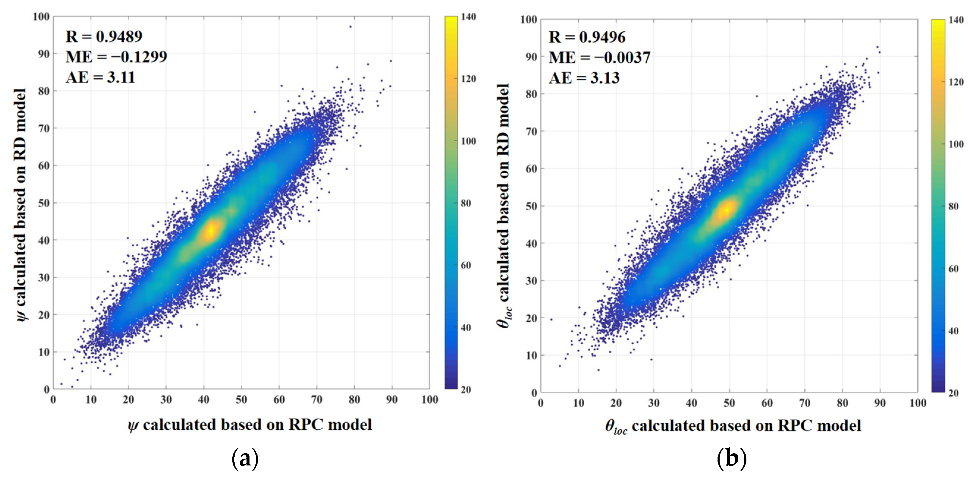
3.2. Local Geometry Angles

The projection angle (ψ) and local incidence angle (θ_loc) are the most important local imaging geometric information in RTC processing. The two angles calculated based on the RPC model in this study are shown in Figure 6 and Figure 7. It can be seen that these two angles have strong spatial consistency with the terrain radiation distortion of the SAR image shown in Figure 5. On the front slope, the value of the local incidence angle is small, but the value of the projection angle is larger, which means that the effective scattering area is larger, so it is brighter on the SAR image. On the back slope, the opposite phenomenon can be seen.

In order to evaluate the accuracy of calculating the local imaging geometric angle based on the RPC model, the calculation results are compared with the angle calculated based on the RD positioning model, as shown in Figure 8. It can be seen that the correlation (R) between the two reached about 0.95, the mean error (ME) was close to 0°, and the absolute error (AE) was about 3°. Here, we can simply calculate the SAR radiation error caused by the angle error of the local imaging geometry according to the correction formula. Take the projection angle as an example, as shown in Figure 8a: the average value of ψ is about 42°. The radiation error of ESA caused by 3° error is about equal to cos(42°) minus cos(45°), that is, about 0.036. Therefore, the influence of 3° angle error on ESA correction is about 3.6%. Similarly, the average value of θ_loc is about 49°. It is assumed that the reference incidence angle is also 49° and that the n is 1. The radiation error of AVE caused by the 3° error is about equal to cos(49°)/cos(49°) minus cos(49°)/cos(52°), that is, about 0.065. Therefore, the influence of the 3° angle error on AVE correction is about 6.5%. It should be noted that the radiation error for the entire RTC process cannot be estimated using the above method due to the complexity of error transmission.

The above results show that the systematic deviation of the angles calculated by the two methods is small, indicating the reliability of the calculation method based on the RPC model. As for the source of absolute error, the possible deviation of image coordinates caused by the two GTC methods may be the main reason.

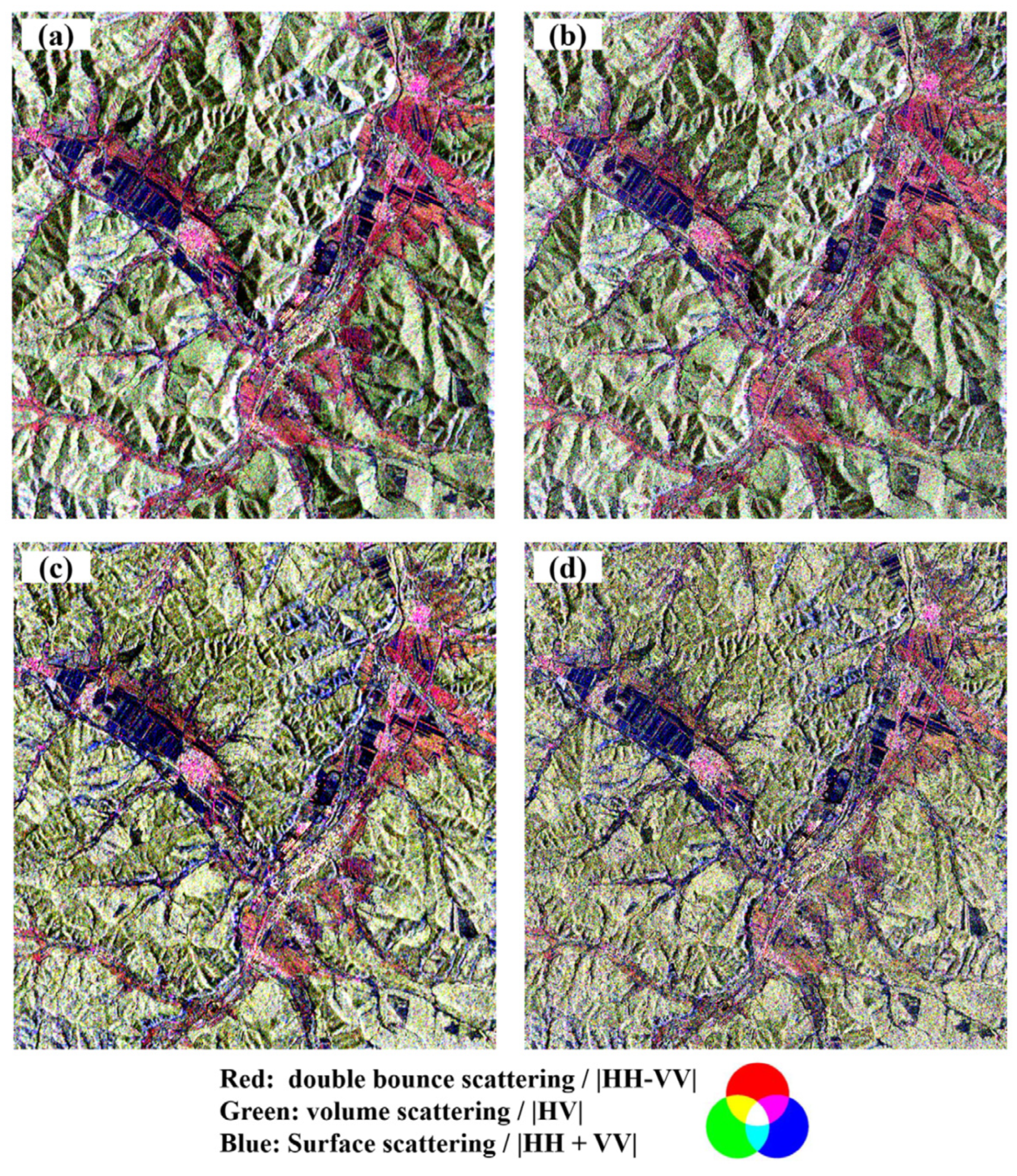
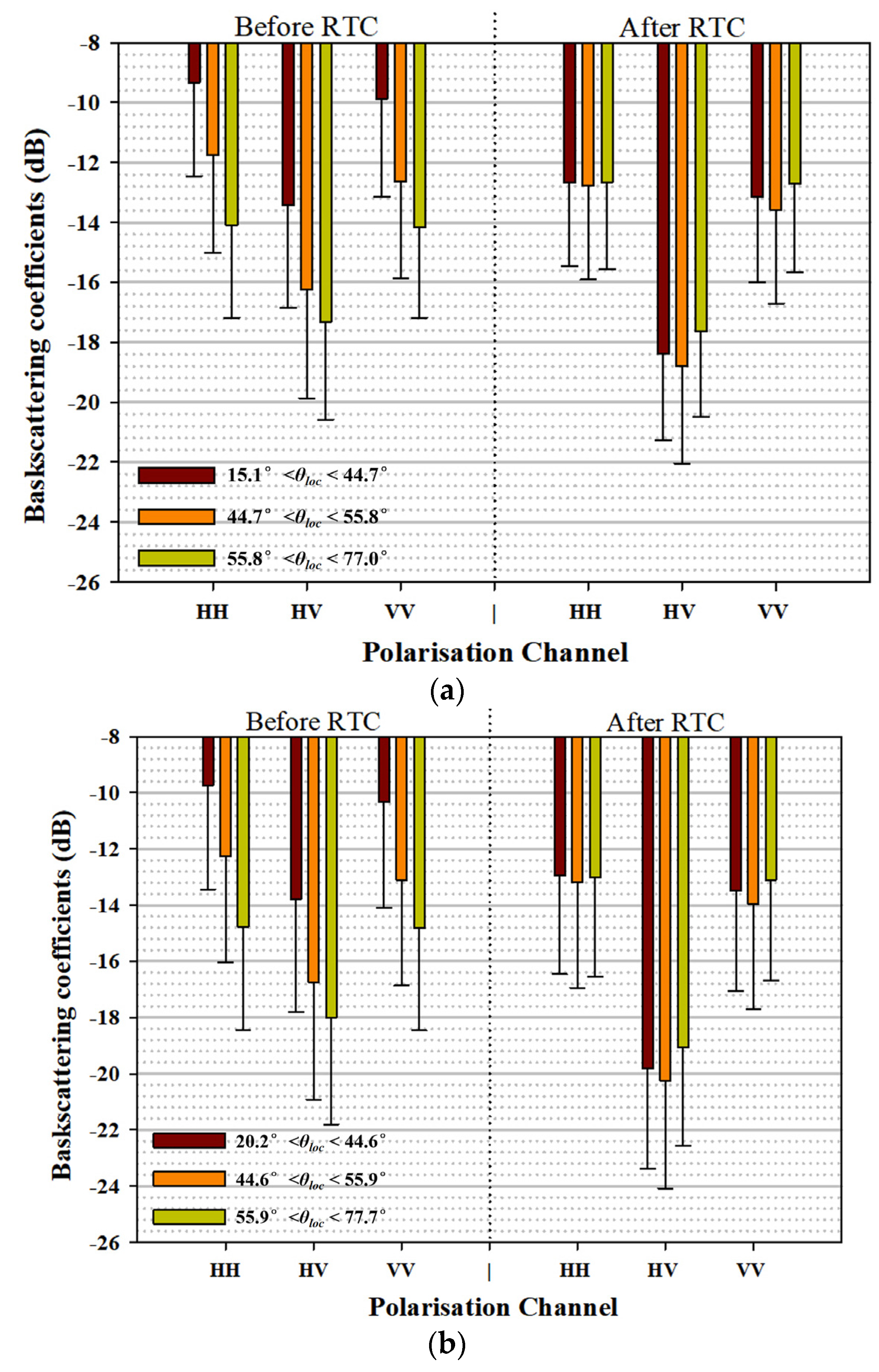
3.3. The RTC Results

Based on the above imaging geometry information, the three-step semi-empirical RTC approach can be realized by using Equation (8). Here, we do not discuss the influence of the n value in AVE correction, so we default the n value of different polarization channels to 1.0, which is often used according to experience. As shown in Figure 9, it is the final RTC correction result based on the RPC model.

It can be clearly seen that the radiation distortion caused by the undulating terrain has been improved, and the obvious difference in backscattering intensity between the front slope and the back slope, as shown in Figure 5, cannot be seen at all. Moreover, after RTC, the mountain forest region presents two distinct characteristics, which in fact represents two types of forest, which also highlights the importance of implementing RTC [5]. This result proves that RTC processing can be well implemented based on the RPC model.

As a comparison, the RTC based on the RD positioning model was also implemented, as shown in Figure 10. Moreover, in order to more clearly display the details of the correction effect, we have provided a partially enlarged image, shown in Figure 11. It can be seen that the RTC correction effect based on the RD positioning model is also good, and no obvious terrain radiation distortion can be seen. The small difference is that the RTC results based on the RPC model are clearer than the RTC results based on the RD model, that is, the noise level of the former is lower. The most likely reason for this phenomenon is the different resampling methods in the GTC process. Bilinear interpolation is used in our program to implement GTC based on the RPC model, while GAMMA software (version: 2012) uses nearest-neighbor interpolation by default. Obviously, the former is because more pixels are used to reduce the noise level by averaging.

In addition, we divided the PolSAR data (before and after RTC) into three groups according to the 33.3rd and 66.6th percentile of the local incidence angle, and the statistical characteristics of different groups and different polarizations are shown in Figure 12. First of all, before RTC, with the change in the local incidence angle, the backscattering coefficient of different polarizations varies greatly, ranging from 4 to 5 dB. After RTC, the difference in the backscattering coefficient of different incident angle groups is reduced to about 0.5 dB. Secondly, in this analysis, the performance of the RPC and RD models is also very consistent. One notable difference is that the mean and standard deviations of the results based on the RD location model are slightly larger. For example, taking HH polarization as an example, the average corrected backscatter coefficient based on the RPC model is approximately 12.4 dB, and the standard deviation is approximately 1.4 to 1.6 dB. The average corrected backscatter coefficient based on the RD model is approximately 12.5 dB, with a standard deviation of approximately 1.6 to 1.9 dB. The lower standard deviation indicates a lower noise level; thus, the resulting RPC-based image will be clearer. The most likely reason is the location deviation of GTC and the different resampling methods.

4. Discussion

Based on the RPC model, this study proposes an RTC method for PolSAR, which is easier to be mastered by remote sensing users. The experiment based on GF-3 PolSAR data shows that this method is effective. In fact, this is a predictable result because the RPC model is essentially an approximate copy of the RD location model. The producer of SAR data solved the RD positioning model before delivering the data to the user and expressed the relationship between the radar slant space and the geographic coordinates with the polynomial of the RPC model [12]. This operation allows SAR users not to have to solve the complex RD positioning model yet achieve a processing effect similar to the RD positioning model. However, there are also some disadvantages: the accuracy of GTC and RTC basically depends on the accuracy of the data producer to solve the RD location model and transform the RPC model. If the user uses a higher-accuracy DEM to solve the RD location model, the effect or accuracy of GTC and RTC may be better.

Moreover, it is possible to optimize the final RTC correction effect in this paper. First, in traditional GTC processing, whether based on the RD positioning model or the RPC model, the accuracy of GTC can be improved by searching the control points between real SAR images and DEM-simulated SAR images [17]. For SAR image processing in mountainous areas, this is a very recommended processing step, and the final RTC effect may also be improved. Reference [16] describes in detail how to simulate SAR images based on the RPC model and improve the orthophoto correction effect. Secondly, the specific method of RTC also has the possibility of optimization. For ESA correction, the projection angle method [7] is the most basic method. If there are more accurate DEM data with higher resolution, the area integration method [18] is a better choice. In addition, for AVE correction, the value of n can be more accurately determined by the minimum correlation coefficient, fitting, and other methods so as to achieve a more precise correction effect.

The main contribution of this article is that it provides an easier alternative technology to the RD localization model for the RTC of PolSAR images. This is of great significance for promoting the application of SAR data in the field of earth observation. Especially for sudden mountain disasters, such as landslides or ice avalanches [19], SAR satellites from a single country often cannot capture images of the disaster area in a timely manner. In such cases, it is often necessary to use SAR data from different countries. However, different countries have different SAR satellite data formats and data processing methods. This has to some extent hindered the application of SAR data. Therefore, the widespread application of SAR data urgently requires simpler and more general processing techniques such as GTC or RTC methods based on the RPC model. In addition, it should be noted that this article only analyzes the impact of RTC correction on the basic features of PolSAR images. In fact, whether to perform RTC has an important impact on applications such as polarization decomposition [20], quantitative parameter inversion [21], and classification [22]. In our previous paper [1], we analyzed in detail the important impact of terrain effects on polarization decomposition. There is a significant linear relationship between the polarization decomposition parameters without RTC and the local incidence angle. In other words, RTC is necessary for polarization decomposition. RTC is more important for classification applications of PolSAR. Research [5] has shown that RTC can improve the classification accuracy of mountain forest types by 20%.

5. Conclusions

In this study, we proposed the RTC approach of PolSAR data based on the RPC model. The main contribution is that we provide a method for calculating the local imaging geometric angle based on the RPC model. Compared with the method based on the RD positioning model, the new method is a lower technical threshold method, which makes it easier for ordinary remote sensing technicians to master it. Moreover, we have shared the program source code for implementing the approach proposed in this study, which can be downloaded from the link in the supplementary materials.

The proposed approach was verified by GF-3 PolSAR data and compared with the method based on the RD positioning model. The following conclusions can be summarized based on the experiments: Firstly, the experimental results of the RTC method based on the RPC model and the RTC method based on the RD positioning model are consistent. For the calculation of local imaging geometry, the difference between the angles calculated based on the RPC model and the RD positioning model is small; that is, the average error is close to 0, and the absolute error is about 3°. Based on this level of angular error, the radiation correction error for ESA correction is approximately 3.6%, and the radiation correction error for AVE correction is approximately 6.5%. Moreover, the RTC approach based on the RPC model is feasible and reliable. Terrain effects in PolSAR images can be effectively removed; specifically, the proposed approach can realize the correction of 4~5 dB terrain radiation distortion to a 0.5 dB level. The above results demonstrate that the proposed RTC method based on the RPC model and the traditional RTC-method-based RD model have similar performance. Therefore, users can use the method proposed in this article to complete the RTC processing of PolSAR data without solving the RD model.

In addition, it should be noted that the method proposed in this paper is only applicable to some of China’s SAR satellites, because only these satellites provide standard RPC files commonly used in optical satellite data. We strongly recommend that other international SAR satellites also provide RPC files, which will greatly reduce the difficulty of SAR data preprocessing and promote the wide application of SAR data.

References

1. Zhao, L.; Chen, E.; Li, Z.; Zhang, W.; Gu, X. Three-Step Semi-Empirical Radiometric Terrain Correction Approach for PolSAR Data Applied to Forested Areas. Remote Sens. 2017, 9, 269. [Google Scholar] [CrossRef] [Green Version]
2. Löw, A.; Mauser, W. Generation of Geometrically and Radiometrically Terrain Corrected SAR Image Products. Remote Sens. Environ. 2007, 106, 337–349. [Google Scholar] [CrossRef]
3. Marc, S.; Bryan, V.R.; Michael, D.; Scott, H. Radiometric correction of airborne radar images over forested terrain with topography. IEEE Trans. Geosci. Remote Sens. 2016, 54, 4488–4500. [Google Scholar]
4. Hoekman, D.H.; Reiche, J. Multi-model radiometric slope correction of SAR images of complex terrain using a two-stage semi-empirical approach. Remote Sens. Environ. 2015, 156, 1–10. [Google Scholar] [CrossRef]
5. Zhao, L.; Chen, E.; Li, Z.; Fan, Y.; Xu, K. The Improved Three-Step Semi-Empirical Radiometric Terrain Correction Approach for Supervised Classification of PolSAR Data. Remote Sens. 2022, 14, 595. [Google Scholar] [CrossRef]
6. Lee, J.S.; Schuler, D.L.; Ainsworth, T.L. Polarimetric SAR data compensation for terrain azimuth slope variation. IEEE Trans. Geosci. Remote Sens. 2000, 38, 2153–2163. [Google Scholar]
7. Ulander, L.M.H. Radiometric slope correction of synthetic-aperture radar images. IEEE Trans. Geosci. Remote Sens. 1996, 34, 1115–1122. [Google Scholar]
8. GAMMA Remote Sensing. Available online: https://www.gamma-rs.ch/ (accessed on 23 February 2023).
9. SNAP (Sentinel Application Platform). Available online: https://docs.csc.fi/apps/snap/ (accessed on 23 February 2023).
10. Zhang, Q.J. System Design and Key Technologies of the GF-3 Satellite. Acta Geod. Cartogr. Sin. 2017, 46, 269–277. [Google Scholar]
11. Zhang, G.; Li, D.; Qin, X.; Zhu, X. Geometric Rectification of High Resolution Spaceborne SAR Image Based on RPC Model. J. Remote Sens. 2008, 12, 942–948. [Google Scholar]
12. Zhang, G.; Fei, W.; Li, Z.; Zhu, X.; Li, D. Evaluation of the RPC Model for Spaceborne SAR Imagery. Photogramm. Eng. Remote Sens. 2010, 76, 727–733. [Google Scholar] [CrossRef]
13. Zhang, G.; Li, Z.; Pan, H.; Qiang, Q.; Zhai, L. Orientation of Spaceborne SAR Stereo Pairs Employing the RPC Adjustment Model. IEEE Trans. Geosci. Remote Sens. 2011, 49, 2782–2792. [Google Scholar] [CrossRef]
14. Zhang, G.; Wu, Q.; Wang, T.; Zhao, R.; Deng, M.; Jiang, B.; Li, X.; Wang, H.; Zhu, Y.; Li, F. Block Adjustment without GCPs for Chinese Spaceborne SAR GF-3 Imagery. Sensors 2018, 18, 4023. [Google Scholar] [CrossRef] [PubMed] [Green Version]
15. Liu, M. A Novel SAR Geocorrection Method Based on RPC model. Remote Sens. Inf. 2014, 29, 77–83. [Google Scholar]
16. Zhang, G.; Qiang, Q.; Zhu, X.; Tang, X. Ortho-rectification of Satellite-borne SAR Image Based on Image Simulation. Acta Geod. Cartogr. Sin. 2010, 39, 554–560. [Google Scholar]
17. Chen, E. Study on Ortho-Rectification Methodology of Space-Borne Synthetic Aperture Radar Imagery. Ph.D. Thesis, Chinese Academy of Forestry, Beijing, China, 2004. [Google Scholar]
18. Small, D. Flattening gamma: Radiometric terrain correction for SAR imagery. IEEE Trans. Geosci. Remote Sens. 2011, 49, 3081–3093. [Google Scholar] [CrossRef]
19. Shugar, D.H.; Jacquemart, M.; Shean, D.; Bhushan, S.; Westoby, M.J. A massive rock and ice avalanche caused the 2021 disaster at chamoli, indian himalaya. Science 2021, 373, eabh4455. [Google Scholar] [CrossRef]
20. Touzi, R. Target Scattering Decomposition in Terms of Roll-Invariant Target Parameters. IEEE Trans. Geosci. Remote Sens. 2006, 45, 73–84. [Google Scholar] [CrossRef]
21. Muhuri, A.; Natsuaki, R.; Bhattacharya, A.; Hirose, A. Glacier surface velocity estimation using stokes vector correlation. In Proceedings of the 2015 IEEE 5th APSAR, Singapore, 1 September 2015. [Google Scholar]
22. Shang, F.; Hirose, A. Quaternion Neural-Network-Based PolSAR Land Classification in Poincare-Sphere-Parameter Space. IEEE Trans. Geosci. Remote Sens. 2014, 52, 5693–5703. [Google Scholar] [CrossRef]
Figure 1. Location of the test site and data coverage of PolSAR data.
Remotesensing 15 01909 g001
Figure 2. The Pauli RGB of PolSAR data over the test site.
Remotesensing 15 01909 g002
Figure 3. The SRTM DEM of the test site.
Remotesensing 15 01909 g003
Figure 4. Local geometry of SAR imaging in an earth-centered rotating (ECR) coordinate system.
Remotesensing 15 01909 g004
Figure 5. The Pauli RGB after GTC based on RPC model.
Remotesensing 15 01909 g005
Figure 6. Projection angle (ψ).
Remotesensing 15 01909 g006
Figure 7. Local incidence angle (θloc).
Remotesensing 15 01909 g007
Figure 8. Calculation accuracy of local imaging geometric angle compared with the angle calculated based on RD model using Gamma software (version: 2012). (a) Projection angle (ψ); (b) Local incidence angle (θloc). ME: Mean Error; AE: Absolute Error.
Remotesensing 15 01909 g008
Figure 9. The Pauli RGB after RTC based on RPC model.
Remotesensing 15 01909 g009
Figure 10. The Pauli RGB after RTC based on RD model using GAMMA software (version: 2012).
Remotesensing 15 01909 g010
Figure 11. The enlarged Pauli RGB: (a) GTC result based on RPC model; (b) GTC result based on RD model; (c) RTC result based on RPC model; (d) RTC result based on RD model.
Remotesensing 15 01909 g011
Figure 12. The statistical characteristics (mean and standard deviation) of backscattering coefficients at different incident angles (grouped by 33.3% and 66.6% quantiles) and different polarizations before and after RTC. (a) Based on RPC model; (b) Based on RD model using GAMMA software (version: 2012).
Remotesensing 15 01909 g012