Fast Factorized Backprojection Algorithm in Orthogonal Elliptical Coordinate System for Ocean Scenes Imaging Using Geosynchronous Spaceborne–Airborne VHF UWB Bistatic SAR

Abstract

Geosynchronous (GEO) spaceborne–airborne very high-frequency ultra-wideband bistatic synthetic aperture radar (VHF UWB BiSAR) can conduct high-resolution and wide-swath imaging for ocean scenes. However, GEO spaceborne–airborne VHF UWB BiSAR imaging faces some challenges such as the geometric configuration, huge amount of echo data, serious range–azimuth coupling, large spatial variance, and complex motion error, which increases the difficulty of the high-efficiency and high-precision imaging. In this paper, we present an improved bistatic fast factorization backprojection (FFBP) algorithm for ocean scene imaging using the GEO satellite-unmanned aerial vehicle (GEO-UAV) VHF UWB BiSAR, which can solve the above issues with high efficiency and high precision. This method reconstructs the subimages in the orthogonal elliptical polar (OEP) coordinate system based on the GEO satellite and UAV trajectories as well as the location of the imaged scene, which can further reduce the computational burden. First, the imaging geometry and signal model of the GEO-UAV VHF UWB BiSAR are established, and the construction of the OEP coordinate system and the subaperture imaging method are proposed. Moreover, the Nyquist sampling requirements for the subimages in the OEP coordinate system are derived from the range error perspective, which can offer a near-optimum tradeoff between precision and efficiency. In addition, the superiority of the OEP coordinate system is analyzed, which demonstrates that the angular dimensional sampling rate of the subimages is significantly reduced. Finally, the implementation processes and computational burden of the proposed algorithm are provided, and the speed-up factor of the proposed FFBP algorithm compared with the BP algorithm is derived and discussed. Experimental results of ideal point targets and natural ocean scenes demonstrate the correctness and effectiveness of the proposed algorithm, which can achieve near-optimal imaging performance with a low computational burden.

1. Introduction

The synthetic aperture radar (SAR) system plays an indispensable role in marine remote sensing, with the applications ranging from shallow water topography mapping to marine military target detection [1,2,3,4,5]. Compared to other sensors such as optical and infrared sensors, the SAR can obtain high-resolution images actively in severe environments and conditions [6]. The conventional SAR system is monostatic, which is relatively simple and easy to implement in terms of geometric configuration and imaging algorithms. However, the bistatic and multi-static SAR systems are becoming increasingly popular due to their greater information acquisition capabilities [7,8,9]. Geosynchronous (GEO) spaceborne–airborne very high-frequency ultra-wideband bistatic synthetic aperture radar (VHF UWB BiSAR) has the advantages of a short revisit period, flexible mobility, wide detection range, good concealment, and strong penetration, and it can carry out high-resolution and wide-swath imaging of ocean scenes [10,11,12]. In recent years, the GEO satellite-unmanned aerial vehicle (GEO-UAV) VHF UWB BiSAR has become a new regime of the BiSAR system, making it a research hotspot [13].

The GEO-UAV VHF UWB BiSAR is a very high-frequency ultra-wideband bistatic SAR system that utilizes the GEO satellite as the transmitter and the passive receivers mounted on the UAV. One of the key advantages of this BiSAR system is its high orbit altitude of approximately 36,000 km, which enables it to provide long-range and long-duration irradiation [14]. Meanwhile, the orbital period of the GEO satellite is synced with the Earth’s rotational velocity, allowing for a revisit period of approximately 24 h compared to the several-day revisit periods typically seen in low earth orbit (LEO) and middle earth orbit (MEO) SAR systems [15]. The remote location of the GEO satellite guarantees the reliable and continuous irradiation for the lightweight, miniaturized, and low-cost UAV, improving the system’s battlefield survivability when performing tasks such as the detection of maritime military targets such as aircraft carriers and warships. Additionally, the flexible flight paths of the UAV and the VHF UWB operating signal enable this BiSAR system to acquire a wealth of oceanic information [16]. However, the GEO-UAV VHF UWB BiSAR is challenged by the special geometry of “far-transmitting and near-receiving”, which can result in issues such as the geometric configuration, huge amount of echo data, synchronization difficulties, serious range–azimuth coupling, large spatial variance, and complex motion error [14,15,16]. These challenges can hinder the efficiency and precision of GEO-UAV VHF UWB BiSAR imaging. In this paper, we mainly focus on the high-efficiency and high-precision algorithm for ocean scenes imaging using the GEO-UAV VHF UWB BiSAR, under the assumption that the GEO satellite and UAV are always time-synchronized and beam-synchronized.

The generation of high-quality SAR images is crucial for a range of SAR applications. To achieve this, the SAR systems transmit electromagnetic waves and receive the reflected waves from the observation scene, which is followed by SAR imaging algorithms that convert the echo signals into SAR images that contain valuable target information. SAR imaging methods can be broadly categorized into two types: time-domain and frequency-domain algorithms [6]. While frequency-domain algorithms tend to be more efficient and have been utilized in BiSAR imaging [17,18,19,20,21], their performance may be limited by factors such as system geometry and platform motion track [22,23]. Additionally, approximations in the calculation process can decrease the precision of frequency-domain algorithms [24]. While the nonlinear chirp scaling (NLCS) algorithm and its extensions have been used in GEO-LEO BiSAR and one-stationary BiSAR imaging [17,22,23,24], they may not be suitable for GEO-UAV VHF UWB BiSAR imaging due to the large accumulation angle and severe range migration associated with the longer synthetic aperture and VHF UWB signal. These issues can cause the NLCS algorithm to encounter difficulties, resulting in large phase errors and reduced imaging precision. To address these issues, an improved omega-k algorithm has been proposed for GEO-airborne BiSAR imaging [25]. However, this model treated the GEO satellite as a stationary transmitter.

Time-domain algorithms are highly regarded for their high imaging precision and can be adapted to a wide range of BiSAR configurations. The bistatic backprojection (BP) algorithm [26] is a well-known time-domain method that calculates the intensity of each point in the SAR image by superimposing the linear transform of each echo at that point. The BP algorithm is well-suited to the GEO-UAV VHF UWB BiSAR, but the point-by-point calculation can be computationally demanding. To reduce the computational burden, several efficient versions of the BP algorithms have been proposed, including the fast BP (FBP) algorithm [27] and fast factorized BP (FFBP) algorithm [28], both of which were originally developed for monostatic SAR imaging and later extended to BiSAR imaging. The FBP algorithm introduces the concept of subapertures and subimages, while the FFBP algorithm recursively fuses the subimages to further reduce the computational burden. There are several studies that have applied the FFBP algorithm to various types of BiSAR systems, including the one-stationary UWB BiSAR [29] and low-frequency narrowband BiSAR [30]. However, few studies have provided implementation details for the bistatic FFBP algorithm. Rodriguez et al. [31] have applied the bistatic FFBP algorithm to spaceborne–airborne BiSAR and were the first to propose reconstructing the subimages in the elliptical polar (EP) system to reduce the computational burden, but this approach was only applicable to linear uniform sampling and required a high angular velocity of the platform. While Vu et al. have provided implementation details and computational complexity analysis for the bistatic FFBP algorithm applied to UWB BiSAR imaging [32], they did not derive the sampling requirements of the subimages. Xie et al. have proposed the bistatic FFBP algorithm for the nonlinear trajectory BiSAR of general configuration and the one-stationary circular BiSAR [33,34], but both approaches require at least one platform’s trajectory to be parallel to the ground. Feng et al. have proposed an FFBP algorithm for the missile-borne BiSAR [35] with the origin of the EP coordinate system determined based on the trajectories of the transmitter and receiver. For GEO spaceborne–airborne BiSAR imaging, a weighted FFBP algorithm was proposed by Wang et al. [14], but the focus of the research was on multi-channel processing, and there were few details provided on the FFBP algorithm. For the forward-looking BiSAR, Pu et al. [36] and Li et al. [37] have proposed an FFBP algorithm integrating the motion trajectory estimation and a non-interpolation FFBP algorithm, respectively. Zhou et al. were the first to propose a bistatic FFBP algorithm that reconstructs the subimage in an orthogonal elliptical polar (OEP) coordinate system [38]. However, their study did not provide implementation details and computational complexity analysis, and it only derived the Nyquist sampling rate of the subimage from the wave number perspective. Building on [38], Bao et al. [39] and Xu et al. [40] analyzed the FFBP algorithm based on the OEP coordinate system from the wave number perspective for airborne BiSAR, but they focused on motion compensation and continuous imaging of large scenes, respectively.

However, the unique geometric configuration of the GEO-UAV VHF UWB BiSAR presents challenges for traditional bistatic FFBP algorithms. This is due to the huge transmit slant range that separates the transmitter from the receiver and imaging scene. In addition, for the high-inclination GEO satellites, the platform speed is usually much larger than the speed of the UAV, and the trajectories of the transmitting and receiving platforms are usually nonlinear due to the orbital characteristics of the GEO satellite and the airflow interference to the UAV. To address these challenges, we propose a modified bistatic FFBP algorithm specifically tailored for the GEO-UAV VHF UWB BiSAR imaging and involves reconstructing the subimages in an OEP coordinate system. This study establishes the OEP coordinate system for the GEO-UAV BiSAR from a three-dimensional perspective and provides an in-depth analysis of the Nyquist sampling requirements from the perspective of phase error, which offer valuable insights for the optimal design of the geometry configuration and system parameters for the GEO-UAV BiSAR system.

The rest of this paper is organized as follows. In Section 2, the imaging geometry and signal models of the GEO-UAV VHF UWB BiSAR are established and analyzed. In Section 3, the establishment of an OEP coordinate system and the application of the bistatic BP algorithm in this coordinate system is proposed. The sampling requirements of the subi-mages in the proposed FFBP algorithm are derived from the perspective of the phase error and demonstrate the computational superiority of the proposed algorithm through sam-pling analysis. The detailed description of the implementation process of the proposed FFBP algorithm is discussed, along with its computational complexity analysis. Experi-ments results are presented in Section 4, including the simulation of ideal point targets and natural scenes. Finally, a conclusion is presented in Section 5.

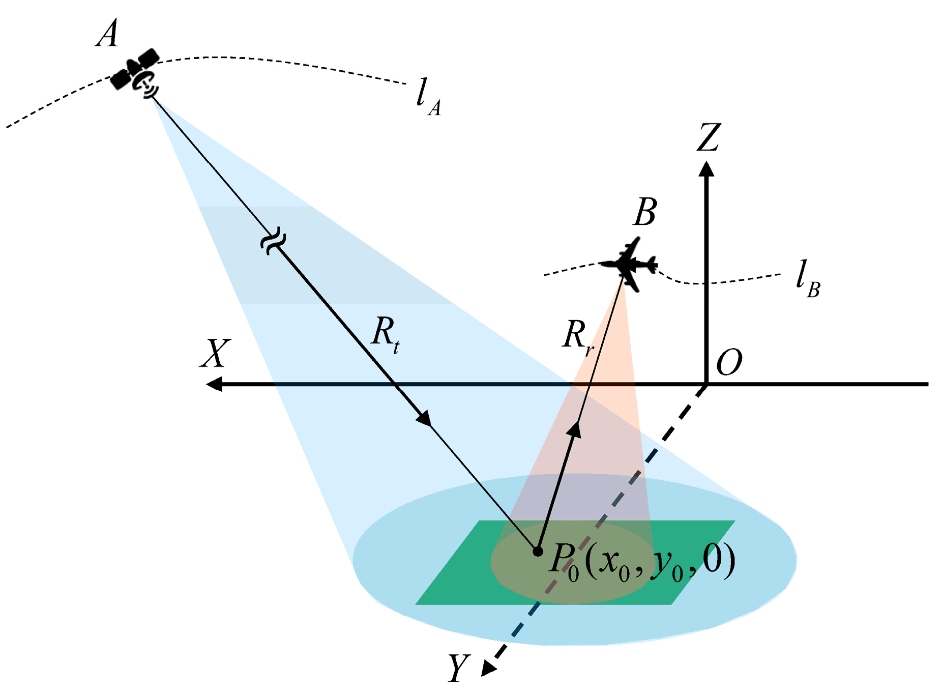
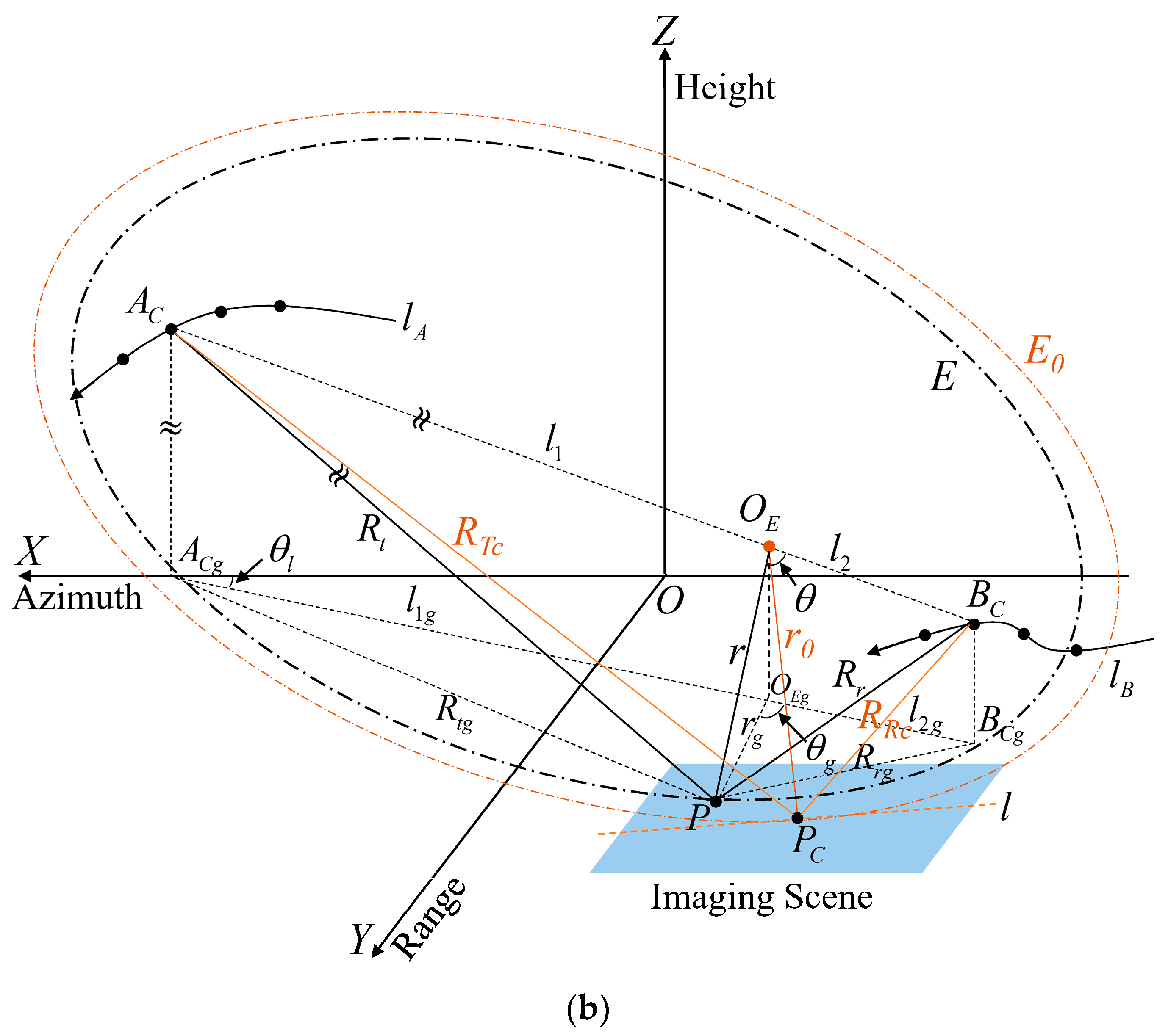
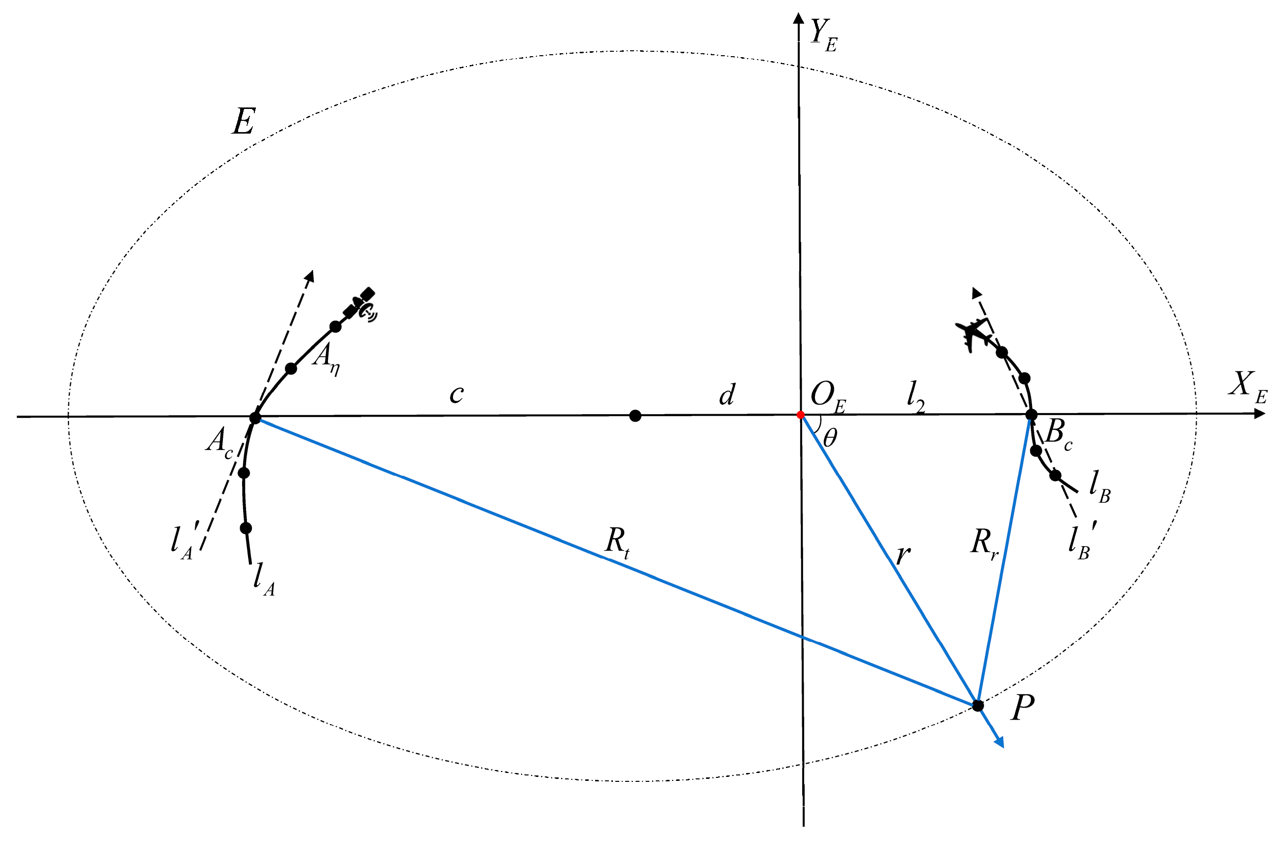
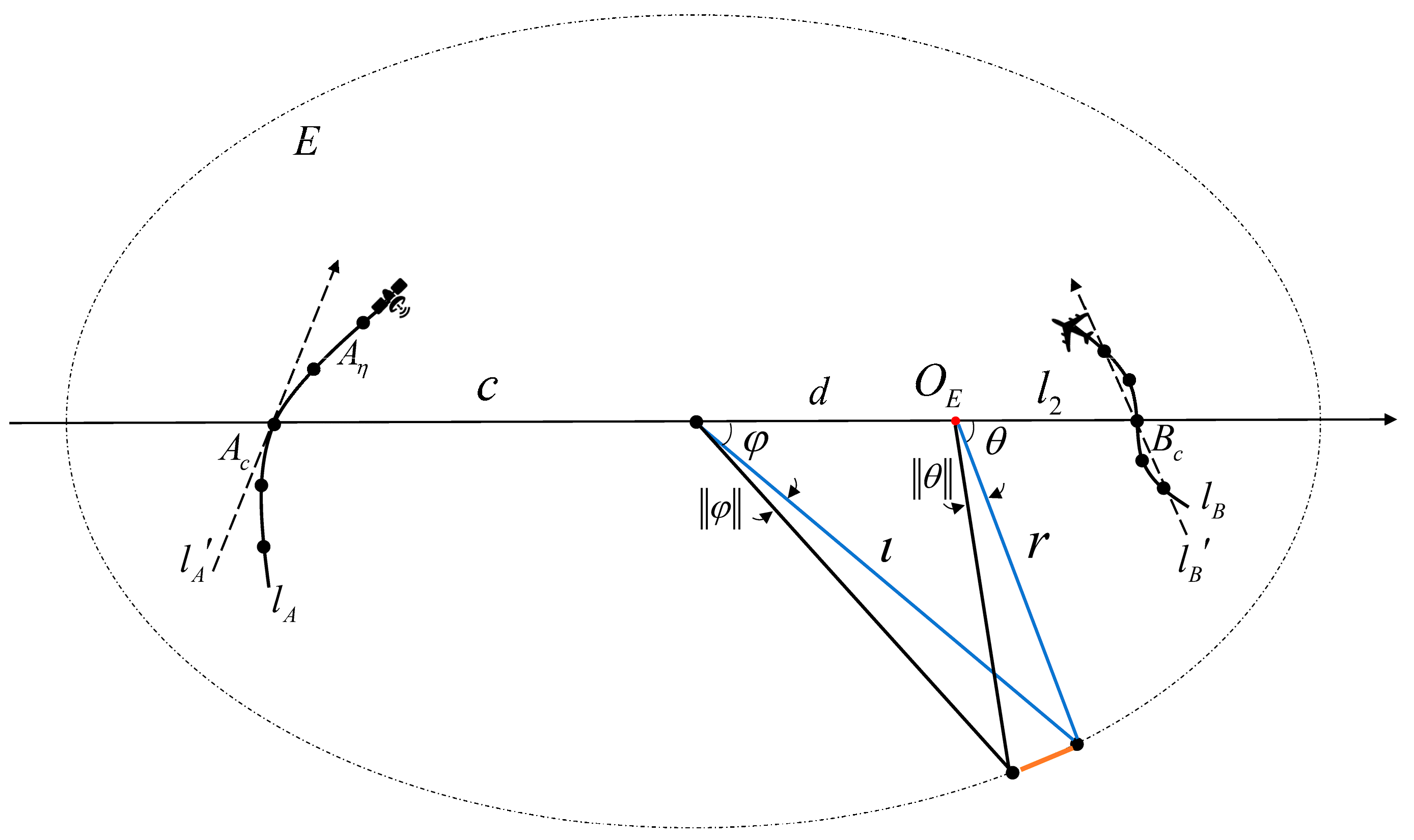
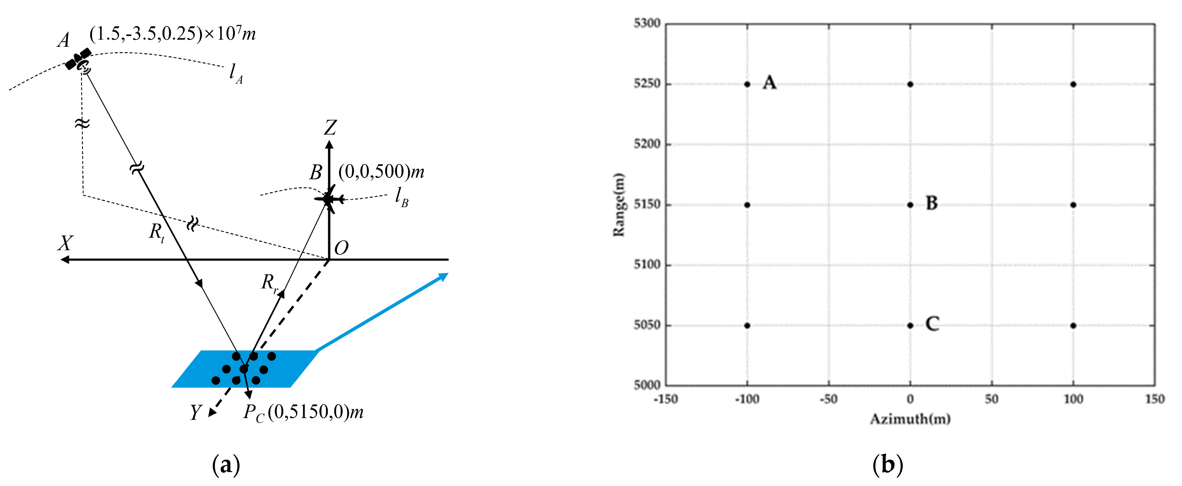
2. Imaging Geometry and Signal Model

The imaging geometry of the GEO-UAV VHF UWB BiSAR system is shown in Figure 1. The system transmitter is mounted on the GEO satellite, and the receiver is mounted on an aircraft flying close to the area of interest. The GEO satellite and the aircraft operate in the spotlight mode and the side-looking strip mode, respectively. It is assumed that the beams of the GEO-UAV BiSAR are always synchronized due to the large beam coverage of the GEO SAR and the limited beam coverage of the UAV. At a given slow time $\eta$, the positions of the transmitter and receiver are $A\left(x_t\left(\eta \right),y_t\left(\eta \right),z_t\left(\eta \right)\right)$ and $B\left(x_r\left(\eta \right),y_r\left(\eta \right),z_r\left(\eta \right)\right)$, respectively. The trajectories of the GEO satellite and UAV are denoted by $l_A$ and $l_B$, respectively. The GEO satellite’s trajectory follows orbital dynamics and is a curve in the synthetic aperture time, while the actual flight trajectory of the receiver carrier is also a curve due to the influence of the airflow and other factors. For any target $P_0\left(x_0,y_0,0\right)$ located in the imaging area, the distance from the transmitter and receiver to the target are $R_t(x_0,y_0;\eta )$ and $R_r(x_0,y_0;\eta )$ at the slow time $\eta$, respectively. The two-way slant distance of the radar pulse transmitted from the transmitter through the target and then received by the receiver is given by

$$R_B\left(x_0,y_0;\eta \right)=\sqrt{{(x}_t\left(\eta \right)-x_0{)}^2+{\left(y_t\left(\eta \right)-y_0\right)}^2+z_t^2\left(\eta \right)}+\sqrt{{(x}_r\left(\eta \right)-x_0{)}^2+{\left(y_r\left(\eta \right)-y_0\right)}^2+z_r^2\left(\eta \right)}$$

(1)

The orbital altitude of the GEO satellite is approximately 36,000 km, which results in the distance $R_t(x_0,y_0;\eta )$ of approximately 10⁷ m from the transmitter to the target $P_0\left(x_0,y_0,0\right)$. On the other hand, the altitude of the UAV typically ranges from the order of 10² m to 10⁴ m, resulting in the receiver being near the target. The transmitting slant range is therefore much larger than the receiving slant range, which is a unique geometric configuration for the GEO-UAV BiSAR imaging. In general, the transmitter transmits a linear frequency-modulated (LFM) signal $p\left(\tau \right)$, which is then received by the receiver after the reflection through the target P₀. After the range compression, the received echo signal becomes

$$s_{rc}\left(\tau ,\eta \right)={\sigma }_{P_0}\cdot p_r\left[B\left(\tau -R_B\left(x_0,y_0;\eta \right)/c_0\right)\right]\cdot \mathrm{e}\mathrm{x}\mathrm{p}\left[-j2\pi f_c{R}_B\left(x_0,y_0;\eta \right)/c_0)\right]$$

(2)

where $\tau$ is the fast time, ${\sigma }_{P_0}$ is the scattering coefficient at the target P₀, $p_r\left(\cdot \right)$ denotes the range-compressed pulse envelop, B denotes the signal bandwidth, f_c denotes the central frequency, and c₀ represents the speed of light.

3. Bistatic FFBP Algorithm in OEP Coordinate System

3.1. Subaperture Imaging

Similar to the conventional FFBP algorithm, the proposed bistatic FFBP algorithm is also based on the subaperture imaging. The full aperture of the transmitter and receiver is divided into several subapertures, and the radar echo data are also divided into the same number of data blocks. The BP algorithm is then applied to each subaperture separately to obtain the corresponding subimages. In the monostatic FFBP algorithm, the echoes are mapped onto a sphere centered on the radar; thus, the subimages are reconstructed in the polar coordinate system instead of the Cartesian coordinate system to reduce the computational burden. In contrast, in the bistatic FFBP algorithm, the echoes are mapped onto an ellipsoidal surface with the transmitter and receiver serving as focal points due to the separation of the transmitter and receiver, and then, the subimages are reconstructed in an ellipsoidal coordinate system. However, in the conventional bistatic FFBP algorithm, the origin of the ellipsoidal polar coordinate system is chosen at the midpoint between the transmitter and receiver, which is more suitable for cases where the slant range difference between the transmitter and receiver is small. For the GEO-UAV bistatic SAR imaging, the UAV operates at a relatively low altitude near the imaging scene, while the distance from the GEO satellite to the imaging scene is much larger. Using the midpoint between the satellite and aircraft as the origin of the ellipsoidal polar coordinate system does not consider the location of the imaging scene, which may significantly increase the computational burden of the FFBP algorithm. To address this issue, an improved ellipsoidal polar coordinate system is proposed for the subaperture processing, in which the origin’s position is jointly determined by the positions of the satellite, aircraft, and imaging scene.

Suppose there are N subapertures in one fusion process. The kth subaperture and subimage grid are demonstrated in Figure 2a, and the subaperture imaging geometry of the kth OEP coordinate system is depicted in Figure 2b. To establish the OEP coordinate system and derive its transformation relationship with the Cartesian coordinate system, the origin of the OEP coordinate system needs to be calculated first.

In Figure 2, $l_A$ and $l_B$ are also the flight trajectories of the GEO satellite and UAV, respectively. The center synthetic time of the kth subaperture is denoted by ${\eta }_c$, and the centers of the subapertures for the satellite and aircraft are, respectively, $A_C\left(x_T,y_T,z_T\right)$ and $B_C\left(x_R,y_R,z_R\right)$. The imaging area is located in the Z-plane in the Cartesian coordinate system, and the center of the imaging scene is $P_C\left(x_c,y_c,0\right)$. The distances from $A_C$ and $B_C$ to $P_C$ are denoted by $R_{Tc}$ and $R_{Rc}$, respectively. An OEP coordinate system is established based on $A_C$, $B_C$ and $P_C$. $E_0$ is the ellipse (the orange dashed line) with $A_C$ and $B_C$ as the focal points and passing through $P_C$. The tangent line l to $E_0$ at $P_C$, with the normal to this tangent line, intersects $A_C{B}_C$ at the point $O_E$. We choose $O_E$ as the origin of the OEP coordinate system. The distance from $O_E$ to $A_C$, $B_C$ and $P_C$ are $l_1$, $l_2$ and $r_0$, respectively. In the ellipse $E_0$ (the black dash–dot line), and let $2c$ be the distance between $A_C$ and $B_C$; then, the eccentricity e is equal to $2c/\left(r_{Tc}+r_{Rc}\right)$. According to the properties of an ellipse, we have $\mathrm{\angle }{A}_C{P}_C{O}_E=\mathrm{\angle }{B}_C{P}_C{O}_E$, so we can obtain the following relationship, i.e.,

$$\left\{\begin{array}{c}{l}_1=e{r}_{Tc}\\ l_2=e{r}_{Rc}\end{array}\right.$$

(3)

Then, the coordinates of $O_E$ can be given by

$$\left\{\begin{array}{c}{x}_O=x_R+\frac{l_2}{2c}\left(x_T-x_R\right)\\ y_O=y_R+\frac{l_2}{2c}\left(y_T-y_R\right)\\ z_O=z_R+\frac{l_2}{2c}\left(z_T-z_R\right)\end{array}\right.$$

(4)

In the second step, the coordinate components of the OEP coordinate system should be selected. $P\left(x,y,0\right)$ represents an arbitrary point in the imaging scene, and the distance from $P$ to $A_C$, $B_C$ and $O_E$ are $R_t$, $R_r$ and $r$, respectively. The polar range component and polar angle component of the point $P$ are defined in the OEP coordinate system as the two-way slant range $\rho$ and the angle $\theta$ between the line $r$ and the main axis of the ellipse, respectively. This can be expressed as follows

$$\left\{\begin{array}{cc}\rho =& R_t+R_r\\ \theta =& \mathrm{a}\mathrm{r}\mathrm{c}\mathrm{c}\mathrm{o}\mathrm{s}\left[\left(r^2+l_2^2-R_r^2\right)/\left(2r{l}_2\right)\right],\theta \in (0,\pi )\end{array}\right.$$

(5)

Figure 3 shows the plane geometry of the elliptical $E$. In this elliptical plane, we have

$$\frac{{\left(x_e+d\right)}^2}{{(\rho /2)}^2}+\frac{y_e^2}{{(\rho /2)}^2-c^2}=1$$

(6)

where $x_e=r\mathrm{c}\mathrm{o}\mathrm{s}\theta$, $y_e=r\mathrm{s}\mathrm{i}\mathrm{n}\theta$ and $d=l_1-c=c-l_2$, which is the offset of the origin from the midpoint of the subaperture centers of the GEO satellite and receiver. After obtaining the relationship between $r$ and $\theta$, then $R_t$ and $R_r$ can be calculated by the cosine theorem, which is given by

$$\left\{\begin{array}{c}{R}_t^2=r^2+l_1^2+2r{l}_1\mathrm{c}\mathrm{o}\mathrm{s}\theta \\ R_r^2=r^2+l_2^2-2r{l}_2\mathrm{c}\mathrm{o}\mathrm{s}\theta \end{array}\right.$$

(7)

.

In the third step, the OEP coordinate system is converted to the Cartesian coordinate system. In Figure 2, let the projections of $A_C$, $B_C$ and $O_E$ onto the $XOY$ plane be $A_{Cg}$, $B_{Cg}$ and $O_{Eg}$, respectively, and the projections of $r$, $R_r$ and $l_2$ onto the $XOY$ plane be $r_g$, $R_{rg}$ and $l_{2g}$, respectively. Then, the coordinates $x$ and $y$ of any point in the imaging scene can be calculated as follows

$$\left\{\begin{array}{c}x=x_O+r_g\mathrm{c}\mathrm{o}\mathrm{s}\left({\theta }_l+{\theta }_g\right)\\ y=y_O+r_g\mathrm{s}\mathrm{i}\mathrm{n}\left({\theta }_l+{\theta }_g\right)\end{array}\right.$$

(8)

where ${\theta }_l$ is the angle between the line $A_{Cg}{B}_{Cg}$ and $X$ axis, which can be calculated as

$${\theta }_g=\mathrm{a}\mathrm{r}\mathrm{c}\mathrm{c}\mathrm{o}\mathrm{s}\left[\left(r_g^2+l_{2g}^2-R_{rg}^2\right)/\left(2r_g{l}_{2g}\right)\right]$$

(9)

According to (5)–(9), the Cartesian coordinates $x$ and $y$ of any point in the imaging scene can be expressed by the OEP coordinates $\rho$ and $\theta$. Then, $R_B\left(x,y;\eta \right)$ can be expressed as a function of $\rho$ and $\theta$, i.e., $R_B\left(x,y;\eta \right)=R_B\left(\rho ,\theta ;\eta \right)$. According to the BP algorithm, for the kth subaperture imaging, the scattering intensity at the sampling point $\left(\rho ,\theta \right)$ is given by

$$I_k\left(\rho ,\theta ;{\eta }_c\right)={\int }_{{\eta }_c-T_k/2}^{{\eta }_c+T_k/2}{s}_{rc}\left(R_B\left(\rho ,\theta ;\eta \right)/c_0,\eta \right)\mathrm{e}\mathrm{x}\mathrm{p}\left(j2\pi f_c{R}_B\left(\rho ,\theta ;\eta \right)/c_0\right)d\eta$$

(10)

where $T_k$ is the synthetic aperture time of the kth subaperture. In practice, both the range-compressed pulse and time data are stored in a discrete form, so the scattering intensity at the sampling point $\left(\rho ,\theta \right)$ in the kth subaperture can be calculated by summing the range-compressed pulse at the corresponding slow time. The integral in (10) should be changed to the accumulation of the range-compressed pulse at the corresponding slow time and can be expressed as

$$I_k\left(\rho ,\theta ;{\eta }_c\right)=\sum _{i=1}^L{s\prime }_{rc}\left(R_B\left(\rho ,\theta ;{\eta }_i\right)/c_0,{\eta }_i\right)\mathrm{e}\mathrm{x}\mathrm{p}\left(j2\pi f_c{R}_B\left(\rho ,\theta ;{\eta }_i\right)/c_0\right)$$

(11)

where L is the number of the sampling points in the corresponding slow time, ${\eta }_i$ is the discrete time, and ${s\prime }_{rc}\left(R_B\left(\rho ,\theta ;{\eta }_i\right)/c_0,{\eta }_i\right)$ is the signal sampling at the time ${\eta }_i$ for $s_{rc}\left(R_B\left(\rho ,\theta ;\eta \right)/c_0,\eta \right)$.

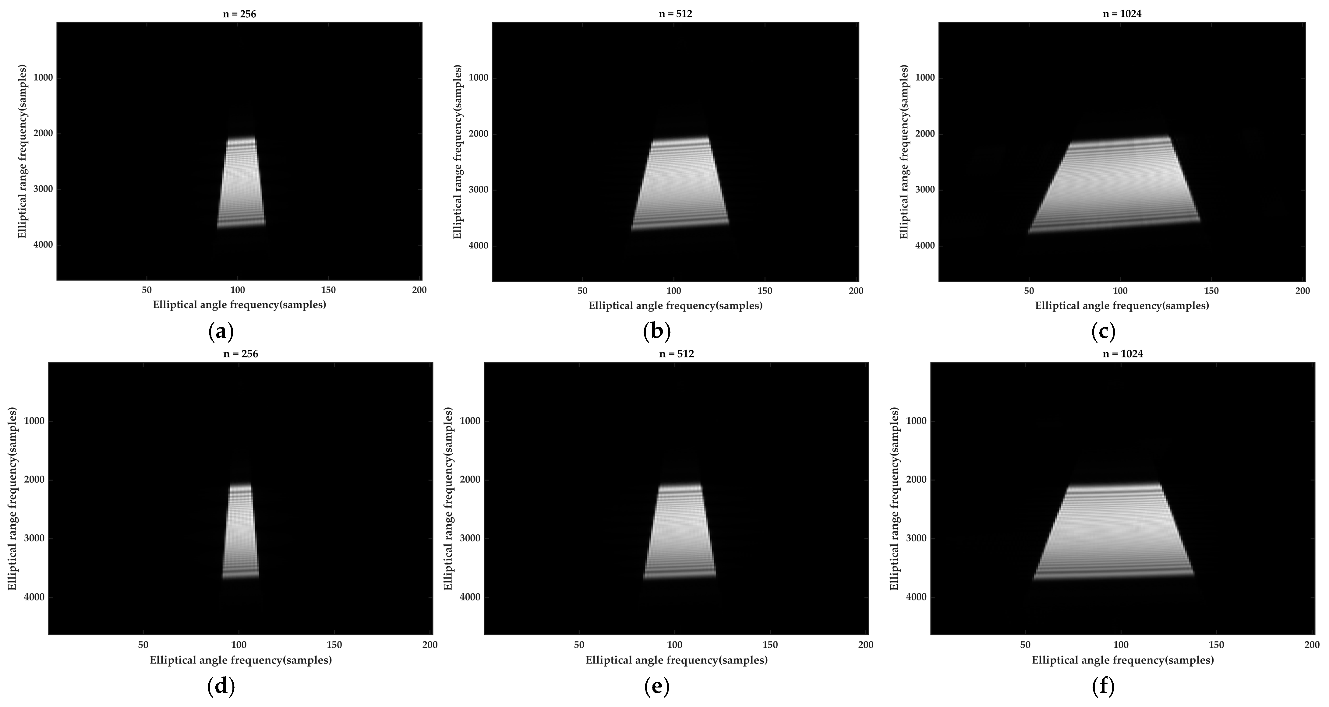
3.2. Sample Requirements

Similar to the conventional FFBP algorithm, the proposed bistatic FFBP algorithm first applies the BP algorithm to the sparser sampling points in the imaging scene at each subaperture to generate lower resolution subimages. In each subsequent stage, the sampling points in the imaging scene are incrementally increased, and the lower resolution subimages from the previous stage are interpolated and fused to obtain higher resolution subimages. Thus, the final SAR image with the desired highest resolution can be obtained through this process. The number of the sampling points at each level of the fusion determines the efficiency and resolution of the imaging algorithm. If the number of sampling points is too small, the required resolution of the imaging results cannot be achieved. If the number of sampling points is too large, it will lead to computational redundancy and significantly increase the computational burden. Therefore, selecting an appropriate sampling requirement at each level of the fusion process is very crucial for balancing the imaging quality with the algorithm performance.

In the monostatic scenario, the SAR image pixels (the imaging scene sampling points), are divided into the azimuth dimension (the platform motion direction) and the range dimension (the vertical direction to the platform motion direction). However, in the GEO-UAV bistatic SAR imaging, due to the separation of the transmitter and receiver and the nonlinear trajectories of both the GEO satellite and aircraft, the concepts of the azimuth and range dimensions are no longer applicable. In the OEP coordinate system, the imaging scene sampling points are divided into the two-way slant range dimension ($\rho$) and the angle dimension ($\theta$). For the two-way slant range dimension, if the system transmits a signal with the bandwidth $B$, the temporal resolution of the system is $1/B$, and the slant range resolution is $c_0/B$, i.e., two adjacent targets can be distinguishable if the difference between their two-way slant range is greater than or equal to $c_0/B$. Therefore, according to the Nyquist’s sampling theorem, the sampling requirement of the two-way slant range dimension in the OEP coordinate system is given by

$$|\Delta \rho |\le c_0/B$$

(12)

For the angular dimension sampling requirement, if the phase error of the antenna caused by the two-way slant range error of two adjacent sampling points in the angular dimension is less than or equal to $\pi /8$, the phase error will only have a minor effect on the sidelobe of the target imaging result under the far-field conditions and can be ignored in the final SAR image. Therefore, the angular dimension sampling requirement can be determined by analyzing the two-way slant range error of the adjacent sampling points in the angular dimension. Figure 4 illustrates the analysis of the two-way slant range error of two adjacent sampling points in the angular dimension in the kth subimage.

In Figure 4, $l_A^{\prime }$ and $l_B^{\prime }$ are the normal linear trajectories of the GEO satellite and aircraft, respectively, while $l_A$ and $l_B$ are their actual trajectories. $A_c$ and $B_c$ are the centers of the lth subapertures, respectively, while $A_{\eta }$ and $B_{\eta }$ are the positions of the satellite and aircraft at the slow time $\eta$, respectively. $P$ and $P_{\pm \Delta \theta }$ are two consecutive sampling points in the imaging scene with the same two-way slant range with the coordinates $\left(\rho ,\theta \right)$ and $\left(\rho ,\theta \pm \Delta \theta \right)$, respectively. $r_{Tc}$ and $r_T$ denote the distance from $A_c$ and $A_{\eta }$ to the target $P$, respectively, the straight-line distance from $A_c$ to $A_{\eta }$ is denoted by ${ϵ}_t$, and the angle between the lines $A_c{A}_{\eta }$ and $r_{Tc}$ is denoted by $\alpha$. Similarly, $r_{Rc}$ and $r_R$ denote the distance from $B_c$ and $B_{\eta }$ to the target P, respectively, the straight-line distance from $B_c$ to $B_{\eta }$ is denoted by ${ϵ}_r$, and the angle between the lines $B_c{B}_{\eta }$ and $r_{Rc}$ is denoted by $\beta$. For the target $P$ at the slow time $\eta$, the two-way slant range of the radar pulse transmitted by the GEO satellite and reflected by the target P to be received by the receiver is given by

$$r_T+r_R=r_{Tc}{\left[1+{\left({ϵ}_t/r_{Tc}\right)}^2-2\left({ϵ}_t/r_{Tc}\right)\mathrm{c}\mathrm{o}\mathrm{s}\alpha \right]}^{\frac{1}{2}}+r_{Rc}{\left[1+{\left({ϵ}_r/r_{Rc}\right)}^2-2\left({ϵ}_r/r_{Rc}\right)\mathrm{c}\mathrm{o}\mathrm{s}\beta \right]}^{\frac{1}{2}}$$

(13)

Expanding the root term in (13) into Taylor series, then (13) can be rewritten as

$$r_T+r_R=r_{Tc}-{ϵ}_t\mathrm{c}\mathrm{o}\mathrm{s}\alpha +\frac{{ϵ}_t^2}{2r_{Tc}}{\mathrm{s}\mathrm{i}\mathrm{n}}^2\alpha +\cdots +r_{Rc}-{ϵ}_r\mathrm{c}\mathrm{o}\mathrm{s}\beta +\frac{{ϵ}_r^2}{2r_{Rc}}{\mathrm{s}\mathrm{i}\mathrm{n}}^2\beta +\cdots$$

(14)

It can be shown that for the sufficiently small values of the subaperture sampling intervals, denoted by ${ϵ}_t$ and ${ϵ}_r$, the two-way slant range $\rho$ can be accurately approximated by neglecting the higher-order terms involving ${ϵ}_t$ and ${ϵ}_r$ in comparison to the terms involving the slant range $r_{Tc}$ and $r_{Rc}$, which can be written as

$$r_T+r_R\approx r_{Tc}+r_{Rc}-{ϵ}_t\mathrm{c}\mathrm{o}\mathrm{s}\alpha -{ϵ}_r\mathrm{c}\mathrm{o}\mathrm{s}\beta$$

(15)

Similarly, for the selected point $P_{\pm \Delta \theta }$, the slant range at the imaging center time and the slow time $\eta$ are represented by $r_{Tc,\pm \Delta \theta }$, $r_{Rc,\pm \Delta \theta }$ and $r_{T,\pm \Delta \theta }$, $r_{Tc,\pm \Delta \theta }$, respectively. Then, the two-way slant range ${\rho }_{\pm \Delta \theta }$ of the sampled point $P_{\pm \Delta \theta }$ at the slow time $\eta$ can be also approximated as

$$r_{T,\pm \Delta \theta }+r_{R,\pm \Delta \theta }\approx r_{Tc,\pm \Delta \theta }+r_{Rc,\pm \Delta \theta }-{ϵ}_t\mathrm{c}\mathrm{o}\mathrm{s}\left(\alpha \pm \Delta \alpha \right)-{ϵ}_r\mathrm{c}\mathrm{o}\mathrm{s}\left(\beta \pm \Delta \beta \right)$$

(16)

where $\Delta \alpha$ and $\Delta \beta$ represent the variation in the angles $\alpha$ and $\beta$, respectively. For the sampling points $P$ and $P_{\pm \Delta \theta }$ within the ellipse E, the two-way slant range is the same (i.e., $r_{Tc}+r_{Rc}=r_{Tc,\pm \Delta \theta }+r_{Rc,\pm \Delta \theta }$). The two-way slant range error for the sampling points P and $P_{\pm \Delta \theta }$ is therefore given by

$$\begin{array}{cc}\Delta r& =\left(r_T+r_R\right)-\left(r_{T,\pm \Delta \theta }+r_{R,\pm \Delta \theta }\right)\hfill \\ & \approx -{ϵ}_t\left[\mathrm{c}\mathrm{o}\mathrm{s}\alpha -\mathrm{c}\mathrm{o}\mathrm{s}\left(\alpha \pm \Delta \alpha \right)\right]-{ϵ}_r\left[\mathrm{c}\mathrm{o}\mathrm{s}\beta -\mathrm{c}\mathrm{o}\mathrm{s}\left(\beta \pm \Delta \beta \right)\right]\hfill \\ & =\pm {ϵ}_t\mathrm{s}\mathrm{i}\mathrm{n}\frac{\Delta \alpha }{2}\mathrm{s}\mathrm{i}\mathrm{n}\left(\alpha \pm \frac{\Delta \alpha }{2}\right)\pm {ϵ}_r\mathrm{s}\mathrm{i}\mathrm{n}\frac{\Delta \beta }{2}\mathrm{s}\mathrm{i}\mathrm{n}\left(\beta \pm \frac{\Delta \beta }{2}\right)\hfill \end{array}$$

(17)

In the ellipse E, $\gamma$ represents the distance between the sampling point P and $P_{\pm \Delta \theta }$. The value of the angle $\Delta \theta$ is usually smaller; thus, the distance $\gamma$ can be approximated as $r\Delta \theta$. Furthermore, we have $\gamma \approx r\Delta \theta \approx r_{Tc}\Delta \alpha \approx r_{R_c}\Delta \beta$. Thus, the relationship between $r_{Tc}$, $r_{Rc}$ and $r$ can be deduced by utilizing the cosine theorem, which is given by

$$\left\{\begin{array}{c}{r}_{Tc}^2=l_1^2+r^2+2l_{1}r\mathrm{c}\mathrm{o}\mathrm{s}\theta \\ r_{Rc}^2=l_2^2+r^2-2l_{2}r\mathrm{c}\mathrm{o}\mathrm{s}\theta \end{array}\right.$$

(18)

Therefore, $\Delta \alpha$ and $\Delta \beta$ can be converted to

$$\left\{\begin{array}{c}\Delta \alpha \approx \frac{r}{r_{Tc}}\Delta \theta =\frac{\left(1-e^2\right)\Delta \theta }{e\mathrm{c}\mathrm{o}\mathrm{s}\theta +\sqrt{1-e^2{\mathrm{s}\mathrm{i}\mathrm{n}}^2\theta }}\\ \Delta \beta \approx \frac{r}{r_{Rc}}\Delta \theta =\frac{\left(1-e^2\right)\Delta \theta }{-e\mathrm{c}\mathrm{o}\mathrm{s}\theta +\sqrt{1-e^2{\mathrm{s}\mathrm{i}\mathrm{n}}^2\theta }}\end{array}\right.$$

(19)

Combining the conditions of $\mathrm{m}\mathrm{a}\mathrm{x}\left[\mathrm{s}\mathrm{i}\mathrm{n}\left(\alpha \pm \frac{\Delta \alpha }{2}\right)\right]=1$ and $\mathrm{m}\mathrm{a}\mathrm{x}\left[\mathrm{s}\mathrm{i}\mathrm{n}\left(\beta \pm \frac{\Delta \beta }{2}\right)\right]=1$, the upper bound on the difference of the two-way slant range is given by

$$|\Delta r|\le \frac{\Delta \theta }{4}\left[\frac{\left(1-e^2\right)d_t}{e\mathrm{c}\mathrm{o}\mathrm{s}\theta +\sqrt{1-e^2{\mathrm{s}\mathrm{i}\mathrm{n}}^2\theta }}+\frac{\left(1-e^2\right)d_r}{-e\mathrm{c}\mathrm{o}\mathrm{s}\theta +\sqrt{1-e^2{\mathrm{s}\mathrm{i}\mathrm{n}}^2\theta }}\right]$$

(20)

where $d_t$ and $d_r$ represent the maximum values of $2{ϵ}_t$ and $2{ϵ}_r$, respectively, which are the lengths of the kth subaperture of the GEO satellite and receiver. To determine the upper bound of $\left|\Delta r\right|$, the values of the angle $\theta$ for several extreme cases of $\left|\Delta r\right|$ have been analyzed. When the values of the angle $\theta$ are 0, $\pi /2$ and $\pi$, respectively, the upper bound of $\left|\Delta r\right|$ becomes

$${\Delta r}_{max}{|}_{\theta =0}=\frac{\Delta \theta }{4}\left[\left(d_t+d_r\right)-e\left(d_t-d_r\right)\right]$$

(21)

$${\Delta r}_{max}{|}_{\theta =\pi /2}=\frac{\Delta \theta }{4}\left[\sqrt{1-e^2}(d_t+d_r)\right]$$

(22)

$${\Delta r}_{max}{|}_{\theta =\pi }=\frac{\Delta \theta }{4}\left[\left(d_t+d_r\right)+e\left(d_t-d_r\right)\right]$$

(23)

In situations where the relative velocity between the transmitter and receiver platforms is not significantly different, i.e., when $d_t$ is not much different from $d_r$, (22) can be chosen as the optimal upper bound for $\left|\Delta r\right|$. However, in the case of the GEO-UAV BiSAR system, the satellite’s velocity is typically much larger than that of the UAV, leading to the fact of $d_r\ll d_t$. In this case, $\left|\Delta r\right|$ calculated according to (23) is the most appropriate choice. To ensure that the phase error caused by the difference in the two-way slant range under far-field conditions is less than or equal to $\pi /8$, the following condition must be satisfied

$$\Delta {\varphi }_{\mathrm{m}\mathrm{a}\mathrm{x}}=\frac{2\pi |\Delta r{|}_{\mathrm{m}\mathrm{a}\mathrm{x}}}{{\lambda }_{\mathrm{m}\mathrm{i}\mathrm{n}}}\le \frac{\pi }{8}$$

(24)

Thus, the angular sampling requirement of the subimages in the OEP coordinate system is given by

$$\Delta \theta \le \frac{c_0}{4\left(f_c+\frac{B}{2}\right)\left[\left(d_t+d_r\right)+e\left(d_t-d_r\right)\right]}$$

(25)

As shown in (25), it can be observed that in the OEP coordinate system, the sampling requirement of the angular dimension of the subimage is only dependent on the eccentricity of the ellipse, which is not affected by the position of the imaging region on the ellipse. In contrast, in the conventional EP coordinate system, the sampling requirement of the angular dimension of the subimage depends not only on the eccentricity of the ellipse but also on the position of the imaging region [31,33]. In the following, the superiority of the subimages in the OEP coordinate system will be analyzed, which would be demonstrated in terms of the sampling requirement in the angular dimension over the conventional EP coordinate system.

3.3. Superiority of Subimages in OEP Coordinate System

There have been numerous studies on the use of the traditional EP coordinate systems in the subimages [35,41]. However, the OEP coordinate system proposed in this paper differs in that its origin is located at the midpoint between the subaperture centers of the transmitter and receiver. Figure 5 illustrates the sampling schematic of the subimages for the same imaging region in both EP and OEP systems.

The orange region within the ellipse E in Figure 5 represents the area to be imaged in this ellipse. The imaged regions in the OEP system and EP system are located at $\theta$ and $\phi$, respectively, while $r$ and $\iota$ represent the polar range in the OEP system and EP system, respectively. In the beamforming and subimage recursive fusion process, it is assumed that the subaperture length of the GEO satellite is significantly larger than that of the receiver (i.e., $d_r\ll d_t$). The two-way slant range sampling requirement of the subimages is the same as that given in (12), while the angular dimension sampling requirement of the subimages is found in [35], which is given by

$$\Delta \phi \le \frac{c_0}{4\left(f_c+\frac{B}{2}\right)\left[d_t/\left(1-\delta \right)+d_r/\left(1+\delta \right)\right]}$$

(26)

where $\delta =c/\iota$ represents the ratio of the elliptical semi-focal distance to the polar range. $\parallel \theta \parallel$ and $\parallel \phi \parallel$ denote the angular sampling range in the OEP system and EP system, respectively. The number of the sampling points in the angular dimension is determined by the ratio of the angular sampling range to the angular sampling rate in each respective coordinate system. $\sigma$ is used to denote the ratio of the number of the angular dimension sampling points in the OEP system to the number of the angular dimension sampling points in the EP system, which is given by

$$\sigma =\frac{\parallel \theta \parallel }{\Delta \theta }/\frac{\parallel \phi \parallel }{\Delta \phi }$$

(27)

Since the range of the image is typically small in comparison to the ellipse, we have $\parallel \theta \parallel r\approx \parallel \phi \parallel \iota$. Therefore, (27) can be rewritten as

$$\sigma \approx \frac{\iota }{r}\frac{\Delta \phi }{\Delta \theta }=\frac{\iota }{r}\frac{\left(d_t+d_r\right)+e\left(d_t-d_r\right)}{d_t/\left(1-\delta \right)+d_r/\left(1+\delta \right)}$$

(28)

In the ellipse E, we take the range of $\phi$ to be $\left(0,\pi /2\right)$; then, the upper and lower bounds of $r$ and $\iota$ are given by

$$\left\{\begin{array}{c}\left(e+1\right)\left(a-c\right)<r<b\\ b<\iota <a\end{array}\right.$$

(29)

From (29), the upper bound of $\sigma$ can be written as

$$\sigma <\frac{a}{\left(e+1\right)\left(a-c\right)}\frac{\left(d_t+d_r\right)+e\left(d_t-d_r\right)}{d_t/\left(1-\delta \right)+d_r/\left(1+\delta \right)}=\frac{1-{\delta }^2}{1-e^2}\frac{\left(d_t+d_r\right)+e\left(d_t-d_r\right)}{\left(d_t+d_r\right)+\delta \left(d_t-d_r\right)}$$

(30)

In the GEO-UAV BiSAR imaging, the imaging scene is typically located near the UAV, i.e., $R_t\gg R_r$. As a result, the values of $\theta$ and $\phi$ are typically within a very small range close to 0. Under these circumstances, $\iota >c$, resulting in $e<\delta <1$. It follows that the two fractions in (30) are less than 1, which leads to $\sigma <1$. This means that for a given imaging area, the number of the angular dimension sampling points in the OEP system is fewer than the number of the angular dimension sampling points in the EP system in the GEO-UAV BiSAR imaging, which can further reduce the computational burden of the bistatic FFBP algorithm.

Figure 6 shows the two-dimensional (2D) spectrum of the imaging result of the single ideal point target in the EP system and OEP system for the subaperture lengths of 256, 512, and 1024, respectively. As seen in Figure 6, the angular dimensional bandwidth of the imaging result of the point target in the OEP system is narrower than that in the EP system. Although the subaperture length increases, the results are the same. To quantify the angular dimensional bandwidth,

Table 1. Two-dimensional (2D) spectrum angular width of the single ideal point target with the different subaperture lengths n.

Subaperture Length	Bistatic EP FFBP (Sampling Point)	Proposed Bistatic FFBP (Sampling Point)	Upgrade Factor
256	25	20	20%
512	61	46	25%
1024	96	80	17%

shows the number of the angular sampling points of the 2D spectrum, which further demonstrates that the proposed FFBP algorithm leads to a narrow width of the angular dimensional spectrum. Therefore, compared to the EP system, reconstructing the subimage of the point target in the OEP system can further reduce the number of the sampling points of the subimages in the angular dimension, which can further improve the efficiency of the bistatic FFBP algorithm.

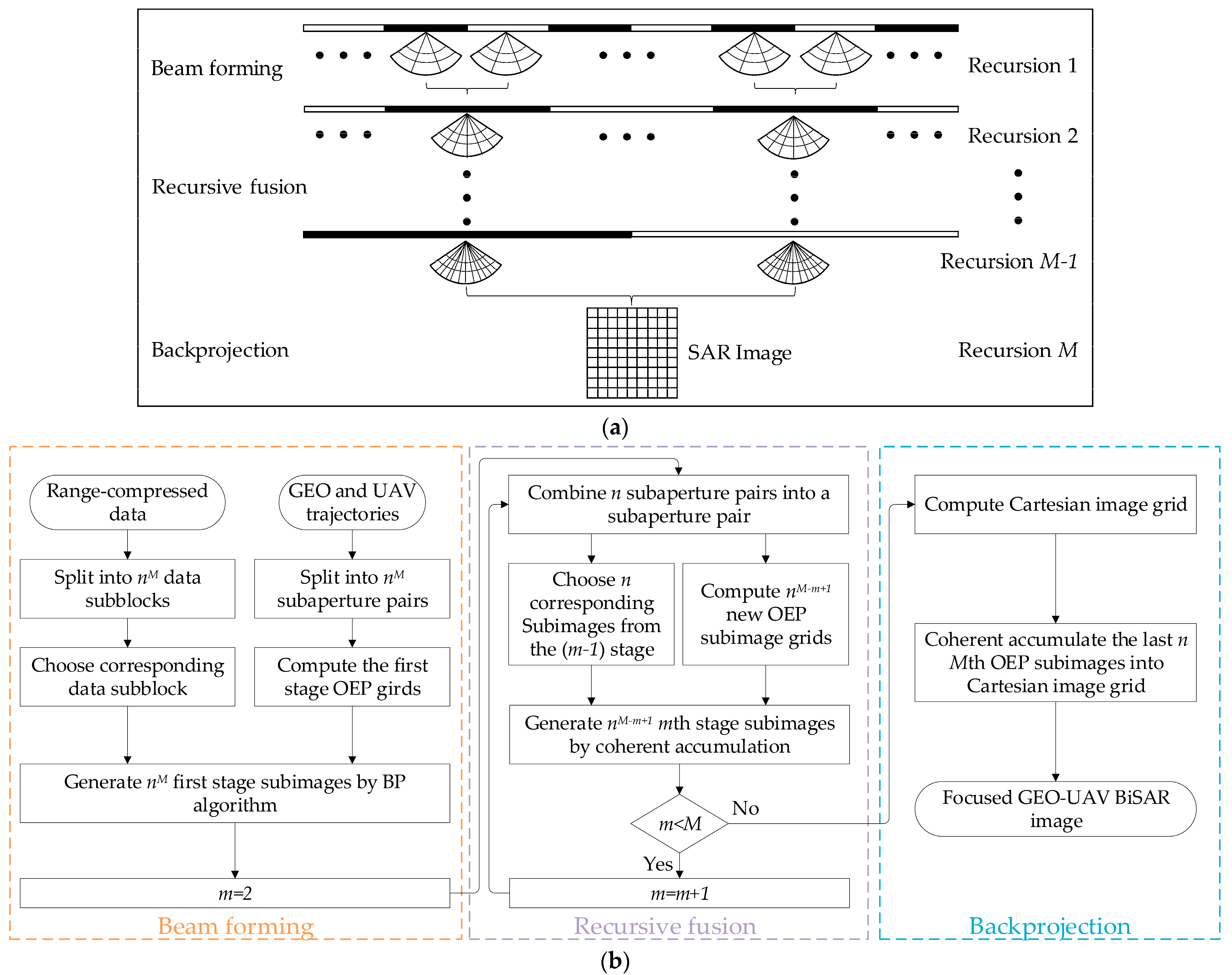
3.4. Implementation Process

The proposed bistatic FFBP algorithm consists of three steps, whose diagram and flow chart are shown in Figure 7. The implementation of this bistatic FFBP algorithm in the OEP system is similar to that of the traditional FFBP algorithm. In general, it involves forming beams [32,42], recursively fusing subapertures, and performing backprojection.

Before the beamforming stage, it is assumed that the full apertures of the GEO satellite and UAV are divided into $n^M$ subapertures, each with a total of $l$ sampling points, and the range-compressed echo data are also divided into the corresponding $n^M$ parts in the slow time. It is important to consider that the number of the subapertures should balance the imaging resolution with the efficiency of the algorithm. If there are too many subapertures, the errors accumulated in the interpolation and fusion stage will increase, leading to a decrease in the imaging quality. However, if the number of the subapertures is too small, the proposed algorithm’s speed advantage will not be fully realized.

Provided that the number of the subaperture pairs of the GEO satellites and UAV combined at each stage of the interpolation fusion is $n$, the total number of the subaperture pairs is $n^{M-m+1}$ after $m$ recursive fusion stages. In the beamforming stage, using the kth first-stage subimage as an example, each pair of the subapertures of the GEO satellite and UAV with the corresponding range-compressed echo data generates a subimage with the lowest resolution using the subaperture imaging algorithm outlined in Section 3.1. The location of the origin of the OEP system is determined by (4) based on the center positions of the subaperture of the GEO satellite and UAV and the center point of the imaging area. Then, the subimage grid is determined according to the Nyquist sampling requirements presented in (12) and (25). Finally, the subimages in the OEP system are obtained by the BP algorithm according to (11), which is given by

$$I_k^1\left({\rho }_k^1,{\theta }_k^1;{\eta }_{kc}^1\right)=\sum _{i=1}^l{s\prime }_{rc}\left(R_B\left({\rho }_k^1,{\theta }_k^1;{\eta }_i^{1,k}\right)/c_0,{\eta }_i^{1,k}\right)\mathrm{e}\mathrm{x}\mathrm{p}\left(j2\pi f_c{R}_B\left(\rho ,\theta ;{\eta }_i^{1,k}\right)/c_0\right)$$

(31)

where ${\rho }_k^1$ and ${\theta }_k^1$ represent the two-way slant range and angular coordinates of the kth subimage in the first stage, respectively, while ${\eta }_{kc}^1$ refers to the subaperture center moment corresponding to that subimage. ${\eta }_i^{1,k}$ represents the slow time of the sampling point within the subaperture time.

In the subaperture recursive fusion stage, the qth subimage of the mth order ($1<m<M$) fusion is taken as an example. Firstly, n adjacent subapertures of the GEO satellite and UAV are fused to form a large subaperture. Then, the origin of the OEP system of the qth subimage is determined based on the center position of the new subaperture pairs and the center point of the imaging area, and the position of the sampling points is also determined according to (12) and (25). As the subaperture length increases, the angular dimensional sampling points in the mth order subimages are denser than in the (m − 1)th order subimages. Finally, the n subimages of the (m − 1)th order are interpolated and superimposed onto the coordinate grid of the qth subimage, respectively. Thus, the low-resolution subimages are fused and superimposed onto the high-resolution subimages. The above process can be summarized as

$$I_q^m\left({\rho }_q^m,{\theta }_q^m\right)=\sum _{p=1+(q-1)n}^{qn}{I}_p^{m-1}\left({\rho }_p^{m-1},{\theta }_p^{m-1}\right)$$

(32)

After (M − 1) recursive fusions, only the last n subapertures and subimages remain. It is worth noting that the sampled points of the previous level subimage may not be exactly the sampled points in the new subimage. Therefore, the values of the sampled points in the new subimage are obtained through the different interpolation methods based on the sampled points around that position in the previous level subimage, which may introduce some errors. As the number of interpolations increases, the errors will also accumulate, causing a degradation in the accuracy of the SAR image. Therefore, the number of the algorithm recursion needs to be controlled. In the backprojection stage, the last n subapertures are superimposed into the full aperture, while the last n subimages are backprojected onto the Cartesian coordinate system in the ground plane to obtain the full-resolution image. We assume that the Cartesian coordinates (x, y) represent any point in the imaging scene, and the sampling points in the x and y directions should be slightly more than the resolution in both directions, respectively. The full-resolution image can be obtained by fusing and superimposing the Mth level subimages, which is expressed as

$$I\left(x,y\right)=\sum _{j=1}^n{I}_j^M\left({\rho }_j^M,{\theta }_j^M\right)$$

(33)

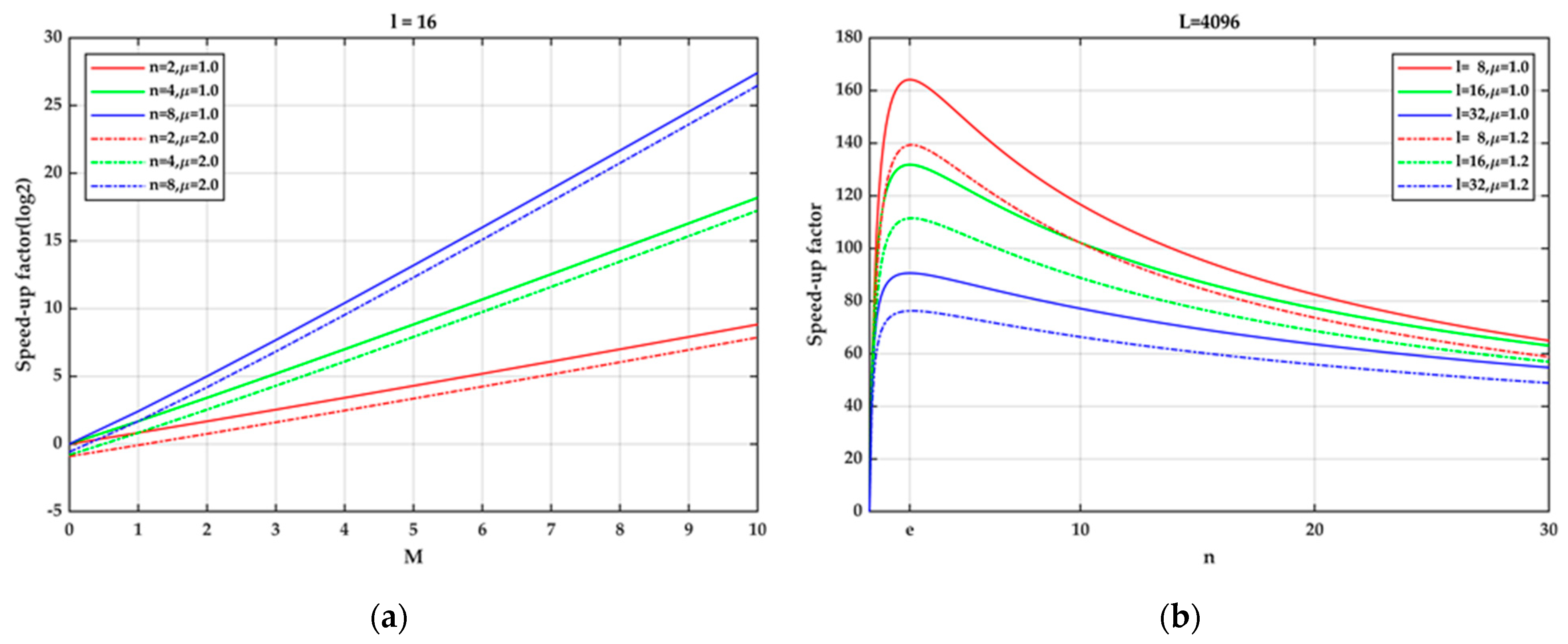
3.5. Computational Burden

To calculate the scattering intensity at the pixel point in the subimage, the following steps must be taken: (1) calculating the coordinates of that point, (2) selecting the surrounding pixel points from the previous level subimage, (3) calculating the compensation phase for the interpolation, and (4) superimposing the pixel points after the compensation phase. We assume that the amount of the total computation needed to calculate one pixel point is $\xi$. It is clear that the amount of computation required for a subimage is proportional to the number of sampling points within it.

To obtain the full-resolution image, the proposed bistatic FFBP algorithm involves three stages: beamforming, recursive fusion and backprojection. The total computation required is the sum of the computation of these three stages. For simplicity, let the full-aperture positions of both the GEO satellite and UAV be L, and let the positions of each subaperture in the first stage (beamforming) be l as well. Furthermore, let the fused subaperture factor in each fusion stage and backprojection stage be a constant n, and let the full-aperture image be obtained after (M − 1) recursive fusions and one backprojection, i.e., $L=l\cdot n^M$. The size of the imaged scene is $N_R\times N_A$ (range x azimuth). In the beamforming stage, the size of each subimage in the OEP system in the two-way slant range and angle dimensions is $N_{\rho ,1}\times N_{\theta ,1}$. Therefore, the total computation required for the subimages in the first stage is given by

$$C_1=n^{M}n{N}_{\rho ,1}{N}_{\theta ,1}\xi =L{N}_{\rho ,1}{N}_{\theta ,1}\xi$$

(34)

During the recursive fusion stage, the number of the fused subimages decreases to 1/n of the original number at each iteration, while the subaperture positions increase to n times the original positions. As a result, the low-resolution subimages are interpolated and fused into the high-resolution subimages. According to (12) and (25), the number of the sampling points in the two-way slant range dimension of the new subimages remains unchanged, but the number of the sampling points in the angular dimension increases to n times the original number, which is due to the increase in the size of the subapertures of both the GEO satellite and UAV. After (m − 1) recursive fusions of the subimages at the mth order $\left(1<m\le M\right)$, the number of the subimages is $n^{M-m+1}$, the positions of the subaperture are $l\cdot n^{m-1}$, and the number of the sampling points in the angular dimension is $n^{m-1}{N}_{\theta ,1}$. Thus, the total computation required for the subimages at the mth order is given by

$$C_m=n^{M-m+1}n{N}_{\rho ,1}{n}^{m-1}{N}_{\theta ,1}\xi =n^{M+1}{N}_{\rho ,1}{N}_{\theta ,1}\xi$$

(35)

As shown in (35), the computation for each order of the subimages is independent of the order in the recursive fusion stage. In the backprojection stage, the last n subimages are directly interpolated into the Cartesian system; thus, the computation is given by

$$C_{M+1}=n{N}_R{N}_A\xi$$

(36)

Provided that the number of the imaging scene sampling points in the Cartesian system is comparable to the number of the imaging scene sampling points in the OEP system in the backprojection stage (i.e., $N_{\rho ,M+1}{N}_{\theta ,M+1}=\mu N_R{N}_A$), the total computational burden of the proposed bistatic FFBP algorithm is given by

$$C_{FFBP}=C_1+{\Sigma }_{m=2}^M{C}_m+C_{M+1}=\left[\left(l+\left(M-1\right)n\right)\mu +n\right]N_R{N}_A\xi$$

(37)

The bistatic BP algorithm requires the calculation of the compensated phase of all pixels in the Cartesian system at each aperture position, which involves multiplying and accumulating them. It is assumed that the computation for each pixel in the BP algorithm is equivalent to that of the proposed bistatic FFBP algorithm; then, the total computation of the bistatic BP algorithm can be written as

$$C_{BP}=L{N}_R{N}_A\xi$$

(38)

Thus, the speed-up factor of the proposed bistatic FFBP algorithm compared with the bistatic BP algorithm is given by

$$\kappa =\frac{C_{BP}}{C_{FFBP}}=\frac{L}{\left[l+\left(M-1\right)n\right]\mu +n}=\frac{L}{\left[l+\left({\mathrm{l}\mathrm{o}\mathrm{g}}_n^{L/l}-1\right)n\right]\mu +n}$$

(39)

From (39), it is shown that the speed-up factor in the proposed bistatic FFBP algorithm is mainly determined by L, M, and n. To analyze the efficiency of the proposed bistatic FFBP algorithm and find the most efficient aperture division method, Figure 8 shows the relationship between the speed-up factor and the number of the fusion times M and the number of fusion apertures n at each order. In Figure 8a, the logarithm of the speed-up factor (base 2) is plotted against the number of fusion orders. When the position of the first subaperture is 16, the larger the full aperture length L, the larger the number of required fusions M. From Figure 8a, it is seen that the speed-up factor is also larger in this case of fusing more subapertures each time with a constant $\mu$. Figure 8b shows that the maximum value of the speed-up factor occurs near the natural logarithm e of the number of the subapertures fused at each stage for a given full aperture length (L = 4096), which decreases with the increasing of n. In practice, however, the number of the subapertures fused at each stage is an integer; thus, n = 2 or n = 3 is optimal. Additionally, the smaller the subaperture of the first stage, the larger the speed-up factor, because more fusions are needed to obtain the full-resolution image, and the computational burden is proportional to the number of the fusions, as shown in Figure 8a. However, in practice, too many recursive fusions will cause the phase error from the interpolation to accumulate, which may lead to a degradation of the image quality. Therefore, it is important to balance the image quality and efficiency by controlling the number of recursive fusions within a reasonable range.

4. Experimental Results and Performance Analysis

To evaluate the correctness and effectiveness of the proposed bistatic FFBP algorithm for the GEO-UAV BiSAR imaging, the experiments have been conducted on both the ideal point targets and natural scenes of the ocean scenes. The bistatic BP algorithm is used as a comparison because it is considered the most accurate SAR imaging algorithm and nearly does not suffer from the phase error effects on the imaging results. The bistatic FFBP algorithm in the EP system is also used to compare the efficiency, which is expressed as the bistatic EP FFBP algorithm in this section for simplicity.

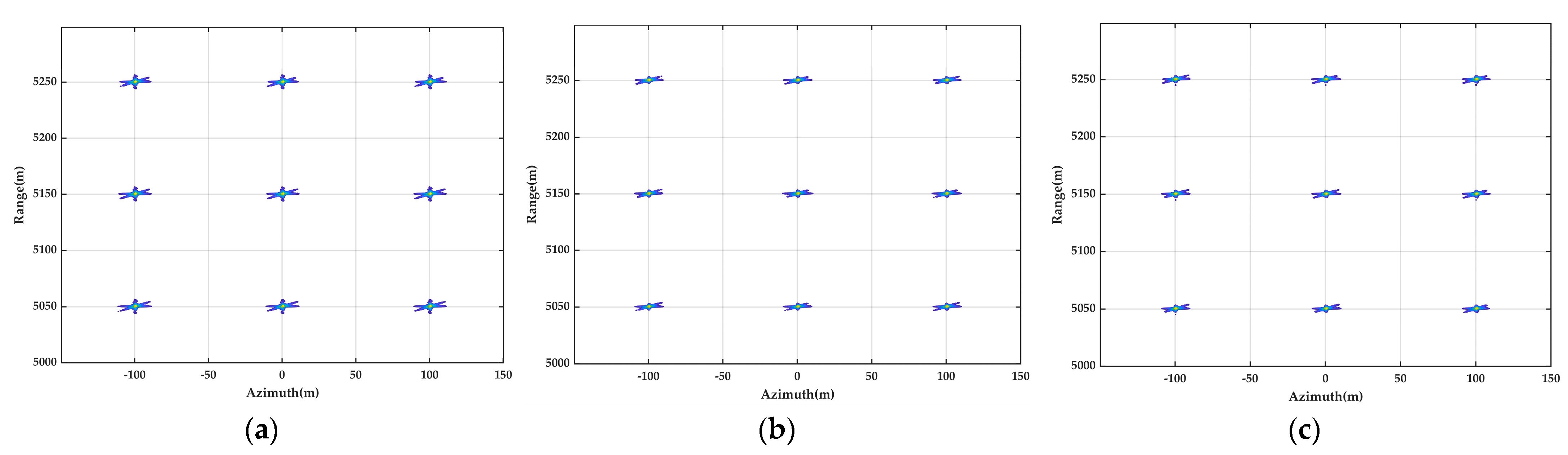
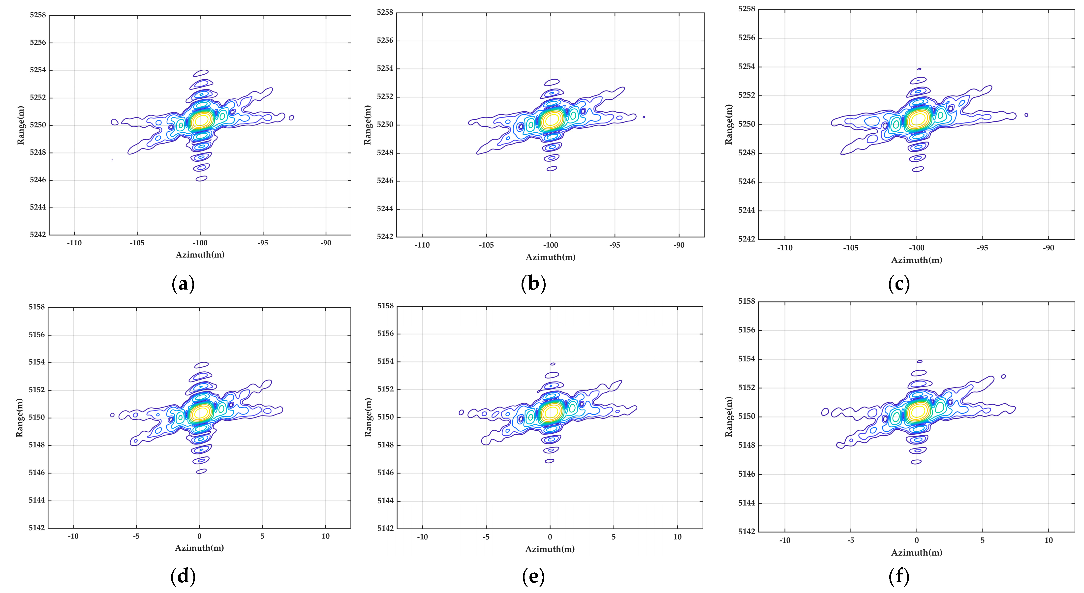
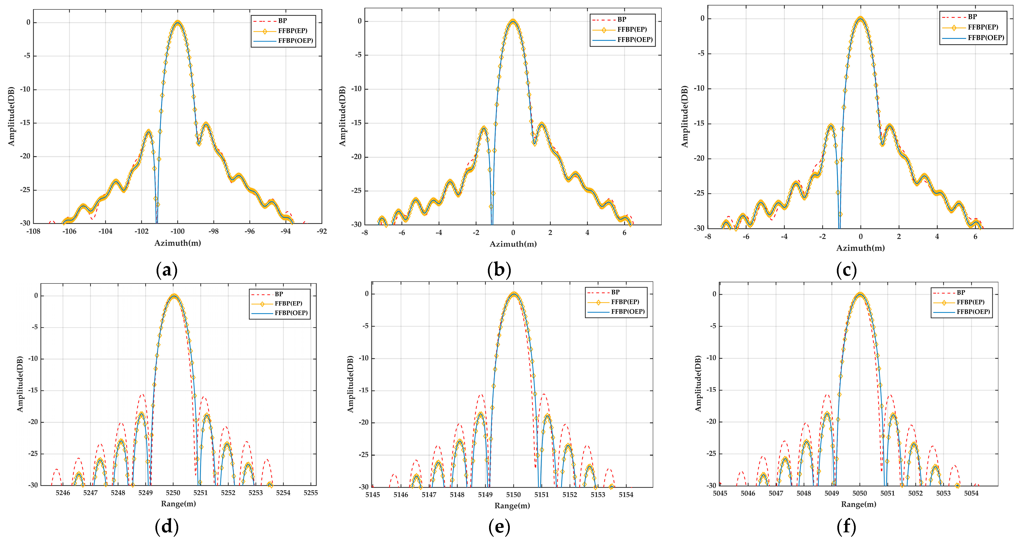
4.1. Experimental Results of Point Targets

Table 2. Experimental parameters for the GEO-UAV VHF UWB BiSAR imaging.

	Parameters	Values	Parameters	Values
BiSAR System	Center frequency	350 MHz	Signal bandwidth	200 MHz
	Pulse duration	1 µs	Pulse repetition frequency	500 Hz
	Sampling frequency	220 MHz	Synthetic aperture time	3.66 s
GEO Satellite	Orbital semi-major axis	42,164 km	Orbital eccentricity	0.005
	Orbital inclination	57°	Perigee argument	90°
	Initial coordinates	(1.5, −3.5, 0.25) × 107 m	Normal velocity	1424.3 m/s
UAV	Height	500 m	Normal velocity	300 m/s
	Initial coordinates	(0, 0, 500) m

lists the experimental parameters for the GEO-UAV BiSAR imaging, and Figure 9a illustrates the geometric schematic for the GEO-UAV BiSAR imaging. The center frequency of 350 MHz and bandwidth of 200 MHz indicate that the GEO-UAV BiSAR system operates in the VHF (P-band) UWB signal.

In the imaging scene, the UAV moves along the positive direction of the X-axis, and the direction parallel to the UAV’s flight direction is defined as the azimuth direction, while the direction perpendicular to the UAV’s flight direction is the range direction (the Y-axis). The UAV operates in the side-looking strip mode with the center of the aperture located at (0, 0, 500)m. The motion error is added to simulate the effects of the airflow and other factors based on the normal linear trajectory of the UAV, with the Y and Z directions representing the UAV’s translational errors (${\delta }_Y=5\mathrm{s}\mathrm{i}\mathrm{n}\left(2\pi \left(1/TA\right)\eta \right)$ and ${\delta }_Z=3\mathrm{s}\mathrm{i}\mathrm{n}\left(2\pi \left(2/TA\right)\eta \right)$), and the X direction representing the UAV’s velocity error (${\delta }_X=2\mathrm{s}\mathrm{i}\mathrm{n}\left(2\pi \left(5/TA\right)\eta \right)$), where TA is the synthetic aperture time. $l_A$ is the flight orbit of the inclined orbit GEO satellite during the synthetic aperture time, which is represented as a curve segment. It is assumed that the GEO satellite is located at (1.5, −3.5, 0.25) × 10⁷ m in the imaging scene at the center of the synthetic aperture, with a slant range of approximately 3.8 × 10⁷. The GEO satellite operates in the spotlight mode, and it is assumed that the transmitter is always beam-synchronized with the receiver due to the large beam coverage of the GEO satellite.

The simulated ocean imaging scene has the dimensions of (300 × 300)m (azimuth × range), with its center located at (0, 5150, 0)m. Nine ideal point targets are placed in the imaging scene, the center point target is located at the midpoint of the imaging scene and the remaining point target is 100 m apart in the range or azimuth direction. The distribution of the point targets is shown in Figure 9b. The radar cross-section (RCS) of each point target is assumed to be 1 m², and the effects of the radar frequency interferometer (RFI), Gaussian white noise, and electromagnetic wave propagation loss are not considered. To objectively evaluate the performance of the imaging algorithms, no window function is used to suppress the side flaps of the imaging results of the point targets.

In the process of the simulation, the number of azimuth sampling points is 4096. For both FFBP algorithms, the initial subaperture length and the number of fused subaperture per time are set to 64 and 4, respectively. Thus, the fusion time is counted as 3. Figure 10 shows the contour plots of the imaging results of the point targets produced by the bistatic BP algorithm, bistatic EP FFBP algorithm, and proposed bistatic FFBP algorithm, respectively. It is seen that all point targets are well-focused, which demonstrates the effectiveness of the proposed bistatic FFBP algorithm. To more clearly observe the details of the focused effects, the imaging results of the point targets, A (corner point), B (center point), and C (marginal point) are extracted and upsampled eight times in the range and azimuth directions using the zero-padding method. Figure 11 displays the impulse response contour maps of the point targets A, B, and C after the upsampling (the left column shows the imaging results using the bistatic BP algorithm, the middle column shows the imaging results using the bistatic EP FFBP algorithm, and the right column shows the imaging results using the proposed bistatic FFBP algorithm). The contour range is [−80, 0] dB, with a step of 4 dB. By comparing the impulse responses of the point targets A, B, and C, it can be seen that the imaging results of the proposed bistatic FFBP algorithm and the bistatic EP FFBP algorithm are both similar to that of the bistatic BP algorithm, and all point targets are well focused at their intended positions. The azimuthal sidelobes are split due to the characteristics of the VHF UWB signal, and the intensity of the two sets of the azimuthal sidelobes is almost equal because the satellite trajectory and the receiver trajectory are roughly parallel. However, the operation of interpolating the lower-resolution subimages to produce the higher-resolution subimages in the proposed bistatic FFBP algorithm introduces the residual phase error. Although the residual phase error is limited to no more than $\pi /8$ during angular dimension sampling and insufficient to affect the mainlobe of the imaging results, it does have a slight impact on the side flaps of the imaging results, as reflected by the purplish-blue contour line ([−80, −30] dB) in Figure 11.

To further compare the effectiveness of the proposed bistatic FFBP algorithm, the range and azimuthal profile analysis has been conducted on the contour maps of the imaging results for the selected point targets, as shown in Figure 12. The range of the profiles is [−30, 0] dB, the red dashed line represents the bistatic BP imaging results, the yellow solid line with diamonds represents the bistatic EP FFBP imaging results, and the blue solid line represents the proposed bistatic FFBP imaging results. For the azimuthal and range profiles of the imaging results for the selected point targets by the proposed bistatic FFBP, the mainlobe completely overlaps with the imaging results by the bistatic BP algorithm, while the sidelobes of the imaging results of the two algorithms differ slightly due to the influence of the residual phase errors. Moreover, the imaging results by the proposed FFBP algorithm are almost the same as the bistatic EP FFBP algorithm for the selected point targets. Both the mainlobe and sidelobe of the imaging results match well, which means that the imaging quality of both bistatic FFBP algorithms is similar.

The imaging performance of the selected point targets can also be quantitatively evaluated using three metrics: resolution (IRW), peak sidelobe ratio (PSLR), and integral sidelobe ratio (ISLR). IRW is the 3 dB width of the mainlobe of the impulse response, PSLR is the ratio of the peak intensity of the sidelobe to the peak intensity of the mainlobe, and ISLR is the ratio of the sum of the sidelobe energies to the energy of the mainlobe.

Table 3. Measured IRW, PSLR and ISLR of the selected targets.

		IRW (m)		PSLR (dB)		ISLR (dB)
		Azimuth	Range	Azimuth	Range	Azimuth	Range
Target A	Bistatic BP	0.96	0.68	−15.31	−15.49	−12.05	−13.35
	Bistatic EP FFBP	0.97	0.73	−15.16	−18.66	−12.03	−16.79
	Proposed bistatic FFBP	0.98	0.74	−15.29	−18.65	−11.90	−16.68
Target B	Bistatic BP	0.95	0.69	−15.37	−15.48	−12.01	−13.32
	Bistatic EP FFBP	0.96	0.74	−15.16	−18.59	−11.89	−16.78
	Proposed bistatic FFBP	0.97	0.74	−14.23	−18.58	−11.61	−16.68
Target C	Bistatic BP	0.95	0.69	−15.40	−15.51	−11.85	−13.34
	Bistatic EP FFBP	0.95	0.74	−15.28	−18.66	−11.84	−16.80
	Proposed bistatic FFBP	0.96	0.73	−15.89	−18.72	−12.02	−16.71

presents the measurement results of the selected point targets in the azimuthal direction and range direction for the three indicators. From Table 3, it is seen that in the azimuthal direction, the imaging results by all three algorithms are nearly identical. In the range direction, the imaging results of the proposed bistatic FFBP algorithm and the bistatic EP FFBP algorithm are very close, as illustrated in Figure 12. In the range direction, compared with the bistatic BP algorithm, the proposed bistatic FFBP algorithm causes a slight widening of the mainlobe width of the impulse response, while the sidelobes peak decreases. Fortunately, the decrease in the range resolution is within an acceptable range in SAR imaging. This phenomenon is due to the effect of the phase error from the interpolation, which could be reduced by increasing the number of the sampling points in the subimage of the OEP system or by choosing a better interpolation method, but this would result in a decrease in imaging efficiency.

To accurately compare the speed-up of the proposed bistatic FFBP algorithm over the bistatic BP algorithm and the bistatic EP FFBP algorithm, the imaging time taken by the three algorithms to the imaging scene of the different sizes is recorded. All imaging algorithms were run on a personal computer with a 2.60 GHz Intel processor and 16 GB of RAM using the Matlab R2022a software. Considering the randomness of a single-time experiment, experiments for each case are conducted five times, respectively, to improve the conviction.

Table 4. Average imaging time of the bistatic BP algorithm, bistatic EP FFBP algorithm and proposed bistatic FFBP algorithm for the imaging scene with the different sizes.

Imaging Scene Size (Azimuth × Range)	Bistatic BP	Bistatic EP FFBP	Proposed Bistatic FFBP	Speed-Up Factor (BP/EP FFBP)
(100 × 100) m	12.69 s	7.67 s	6.82 s	1.86/1.12
(300 × 300) m	84.13 s	19.63 s	15.88 s	5.30/1.24
(500 × 500) m	219.53 s	36.58 s	29.11 s	7.61/1.26

shows the average imaging time required for the different scene sizes and the corresponding speed-up factors for each imaging algorithm. From Table 4, it is evident that the proposed bistatic FFBP algorithm has a significant improvement in the imaging speed compared to the bistatic BP algorithm for the different sizes of imaging scenes, which is consistent with the analysis in Section 3.5. In addition, due to the reduction in the angular dimension sampling points of the subimages, the proposed bistatic FFBP algorithm can improve the efficiency of the bistatic EP FFBP algorithm by about 10–30%, which is consistent with the upgrade factors in Table 1. Moreover, the speed-up factor gradually increases as the size of the imaging scene increases; i.e., the larger the imaging scene, the higher the imaging efficiency of the proposed bistatic FFBP algorithm compared to the other two algorithms. Therefore, the proposed bistatic FFBP algorithm is well-suited for the high-efficiency and high-resolution imaging in a large scene.

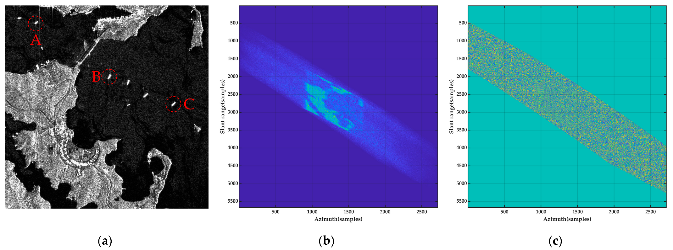
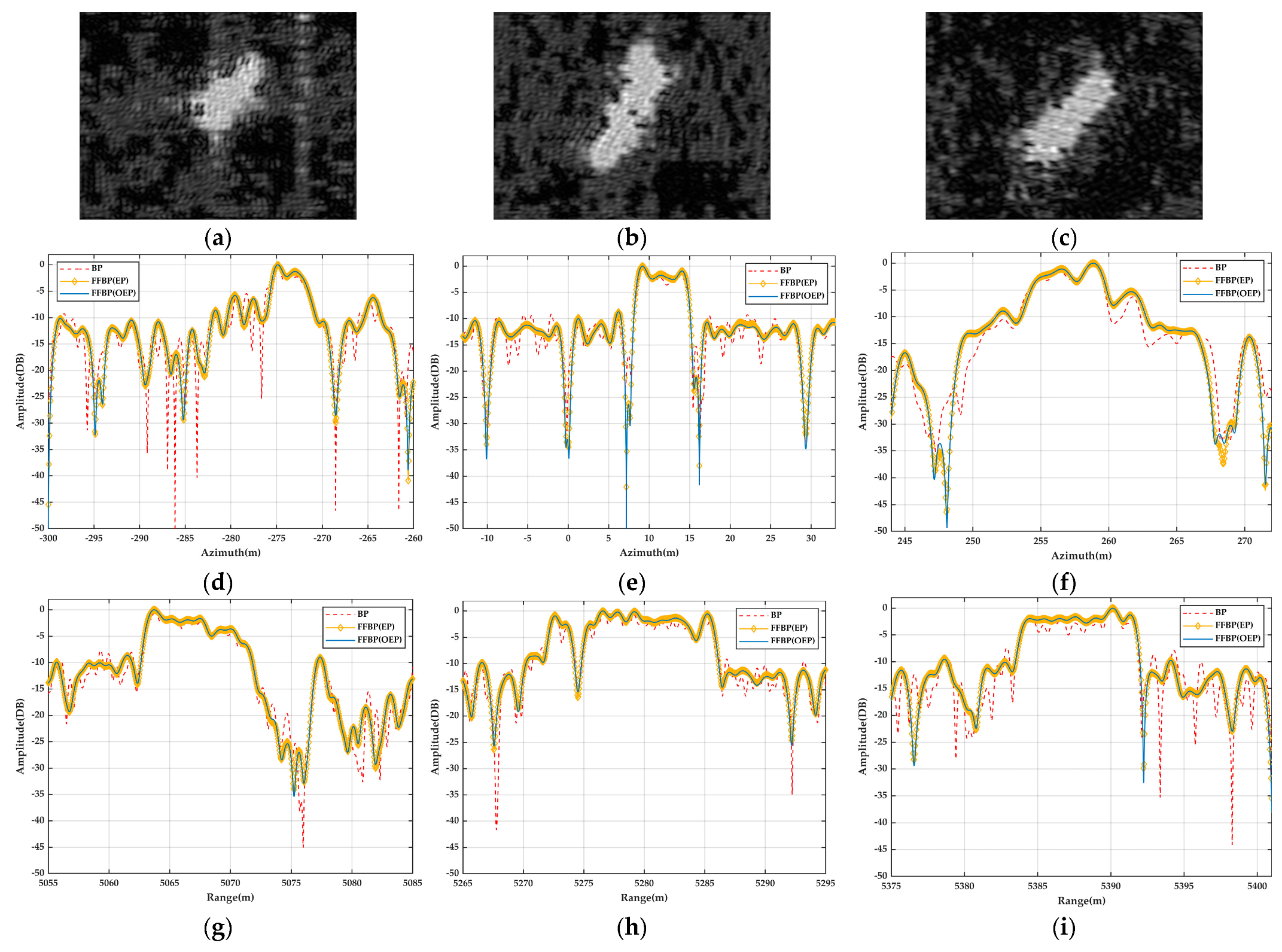
4.2. Experimental Results of Natural Scene

To further verify the effectiveness and efficiency of the proposed bistatic FFBP algorithm, simulation results of the three algorithms for the natural scene echoes are given. According to the studies in [9,43], the pixel gray values of the SAR images can be regarded as the electromagnetic backward-scattering coefficients of the natural scenes. Thus, the SAR images can simulate the scattering characteristics of the natural scenes. In this section, the SAR image used in the experiment contains the natural scenes such as the ocean as well as the docks and ships, with a scene size of 2.4 km × 2.4 km and resolution of 5 m × 5 m, as shown in Figure 13a. In the process of generating echoes, since the pulse by pulse and target-by-target (TBT) algorithm is the most accurate algorithm and has no approximation [9], it is used to generate the echoes of the ocean natural scene with the center of the scene located at (0, 5400)m according to the parameters of the GEO-UAV VHF UWB BiSAR system given in Table 2. The amplitude and phase of the echo signal of this ocean scene are given in Figure 13b,c.

For both FFBP algorithms, the fusion time and number of fused subaperture per time are both set to be 4. The reconstructed SAR images of this natural scene echo signal using the bistatic BP algorithm, the bistatic EP FFBP algorithm, and the proposed bistatic FFBP algorithm are shown in Figure 14a–c, respectively. As shown in Figure 14, the reconstructed SAR images obtained using the three algorithms are all well-focused, and the ships, bridges, and docks are clearly distinguished. Compared to the real ocean SAR image, the contrast of the reconstructed SAR images slightly decreases, since the number of the image pixels increases. However, the reconstructed SAR images obtained using the three algorithms are identical, and it is hard to find any difference. To further explore the imaging quality, three ship targets in the red circle in Figure 13a are extracted to produce their azimuthal and range profiles, which are illustrated in Figure 15. It is seen that the profile curves of the three algorithms are basically consistent in both the azimuthal and range directions. Similarly, the results generated by the bistatic BP algorithm are still the most accurate, since they have higher sensitivity and resolution, which leads to better performance than the other two algorithms. Moreover, the profile curves obtained by the bistatic EP FFBP algorithm and the proposed bistatic FFBP algorithm are coincident. The reason is that the number of the subimage fusions during the imaging process is the same, thus resulting in an equal residual phase error. Fortunately, the residual phase error caused by the interpolation does not seriously affect the imaging quality in this case.

From the perspective of the algorithm efficiency, the average imaging times of five experiments of the bistatic BP algorithm, the bistatic EP FFBP algorithm, and the proposed bistatic FFBP algorithm are 354.00 s, 67.57 s, and 39.10 s, respectively. The speed-up factor of the proposed bistatic FFBP algorithm over the bistatic BP algorithm and the bistatic EP FFBP algorithm are 9.05 and 1.73, respectively. The improvement over the point targets simulation is due to the increase in the number of fusion times and subaperture lengths. Therefore, the proposed bistatic FFBP algorithm is almost the same as the BP algorithm in terms of imaging quality, but the imaging efficiency is further improved compared with the bistatic EP FFBP algorithm, which is the optimal imaging algorithm in large natural ocean scenes.

5. Conclusions

In this paper, we present an improved bistatic FFBP algorithm for reconstructing the GEO-UAV BiSAR images of the ocean scenes with high efficiency and high precision. Different from the conventional FFBP algorithm, the proposed bistatic FFBP algorithm reconstructs the subimages in an OEP system to further reduce the computational burden. First, the origin of the OEP system of the proposed bistatic FFBP algorithm is determined by the positions of the GEO satellite, UAV, and observed imaging scene simultaneously, which can reduce the angular dimensional sampling rate of the subimages. This paper provides details on the method for establishing the OEP system and the subaperture imaging method in the proposed bistatic FFBP algorithm. Moreover, this paper presents the analytical derivation of the Nyquist sampling requirement of the OEP subimage in the two-way slant range and angular dimension and then demonstrates the superiority of the sampling rate in the angular dimension using the OEP system compared to the conventional FFBP algorithm through the simulation experiments. In addition, this paper describes the implementation details and computational complexity of the proposed bistatic FFBP algorithm. It is seen that the proposed bistatic FFBP algorithm has a higher efficiency than the bistatic BP algorithm. Finally, the imaging experiments were conducted on the ideal point targets and natural ocean scenes, which shows that the proposed bistatic FFBP algorithm has almost no loss in the imaging precision, but it significantly improves the imaging efficiency, thereby demonstrating the effectiveness of the proposed algorithm.

References

1. Dai, Z.; Li, H.; Liu, D.; Wang, C.; Shi, L.; He, Y. SAR Observation of Waves under Ice in the Marginal Ice Zone. J. Mar. Sci. Eng. 2022, 10, 1836. [Google Scholar] [CrossRef]
2. Ni, W.; Stoffelen, A.; Ren, K. Tropical Cyclone Wind Direction Retrieval from Dual-Polarized SAR Imagery Using Histogram of Oriented Gradients and Hann Window Function. IEEE J. Sel. Top. Appl. Earth Obs. Remote Sens. 2022, 16, 878–888. [Google Scholar] [CrossRef]
3. Sun, Z.; Meng, C.; Cheng, J.; Zhang, Z.; Chang, S. A Multi-Scale Feature Pyramid Network for Detection and Instance Segmentation of Marine Ships in SAR Images. Remote Sens. 2022, 14, 6312. [Google Scholar] [CrossRef]
4. Xie, H.; Jiang, X.; Hu, X.; Wu, Z.; Wang, G.; Xie, K. High-Efficiency and Low-Energy Ship Recognition Strategy Based on Spiking Neural Network in SAR Images. Front. Neurorobot. 2022, 16, 970832. [Google Scholar] [CrossRef]
5. Jiang, X.; Xie, H.; Chen, J.; Zhang, J.; Wang, G.; Xie, K. Arbitrary-Oriented Ship Detection Method Based on Long-Edge Decomposition Rotated Bounding Box Encoding in SAR Images. Remote Sens. 2023, 15, 673. [Google Scholar] [CrossRef]
6. Xie, H.; Hu, J.; Duan, K.; Wang, G. High-Efficiency and High-Precision Reconstruction Strategy for P-Band Ultra-Wideband Bistatic Synthetic Aperture Radar Raw Data Including Motion Errors. IEEE Access 2020, 8, 31143–31158. [Google Scholar] [CrossRef]
7. Ulander, L.M.H.; Barmettler, A.; Flood, B.; Frölind, P.-O.; Gustavsson, A.; Jonsson, T.; Meier, E.; Rasmusson, J.; Stenström, G. Signal-to-Clutter Ratio Enhancement in Bistatic Very High Frequency (VHF)-Band SAR Images of Truck Vehicles in Forested and Urban Terrain. IET Radar Sonar Navig. 2010, 4, 438. [Google Scholar] [CrossRef]
8. An, D.; Chen, L.; Huang, X.; Zhou, Z.; Feng, D.; Jin, T. Bistatic P Band UWB SAR Experiment and Raw Data Processing. In Proceedings of the 2016 CIE International Conference on Radar (RADAR), Guangzhou, China, 10–13 October 2016; pp. 1–4. [Google Scholar]
9. Xie, H.; An, D.; Huang, X.; Zhou, Z. Efficient Raw Signal Generation Based on Equivalent Scatterer and Subaperture Processing for One-Stationary Bistatic SAR Including Motion Errors. IEEE Trans. Geosci. Remote Sens. 2016, 54, 3360–3377. [Google Scholar] [CrossRef]
10. Cui, C.; Dong, X.; Chen, Z.; Hu, C.; Tian, W. A Long-Time Coherent Integration STAP for GEO Spaceborne-Airborne Bistatic SAR. Remote Sens. 2022, 14, 593. [Google Scholar] [CrossRef]
11. Dong, X.; Cui, C.; Li, Y.; Hu, C. Geosynchronous Spaceborne-Airborne Bistatic Moving Target Indication System: Performance Analysis and Configuration Design. Remote Sens. 2020, 12, 1810. [Google Scholar] [CrossRef]
12. Xu, W.; Wei, Z.; Huang, P.; Tan, W.; Liu, B.; Gao, Z.; Dong, Y. Azimuth Multichannel Reconstruction for Moving Targets in Geosynchronous Spaceborne–Airborne Bistatic SAR. Remote Sens. 2020, 12, 1703. [Google Scholar] [CrossRef]
13. Sun, Z.; Wu, J.; Pei, J.; Li, Z.; Huang, Y.; Yang, J. Inclined Geosynchronous Spaceborne–Airborne Bistatic SAR: Performance Analysis and Mission Design. IEEE Trans. Geosci. Remote Sens. 2016, 54, 343–357. [Google Scholar] [CrossRef]
14. An, H.; Wu, J.; He, Z.; Li, Z.; Yang, J. Geosynchronous Spaceborne–Airborne Multichannel Bistatic SAR Imaging Using Weighted Fast Factorized Backprojection Method. IEEE Geosci. Remote Sens. Lett. 2019, 16, 1590–1594. [Google Scholar] [CrossRef]
15. Wu, J.; Sun, Z.; An, H.; Qu, J.; Yang, J. Azimuth Signal Multichannel Reconstruction and Channel Configuration Design for Geosynchronous Spaceborne–Airborne Bistatic SAR. IEEE Trans. Geosci. Remote Sens. 2019, 57, 1861–1872. [Google Scholar] [CrossRef]
16. Wang, Z.; Li, Y.; Li, Y.; Zhao, J.; Huang, Y.; Shao, S. Research on Compound Scattering Modeling and Imaging Methods of Sea Surface Ship Target for GEO-UAV BiSAR. In Proceedings of the 2022 3rd China International SAR Symposium (CISS), Shanghai, China, 2–4 November 2022; pp. 1–5. [Google Scholar]
17. Qiu, X.; Hu, D.; Ding, C. An Improved NLCS Algorithm With Capability Analysis for One-Stationary BiSAR. IEEE Trans. Geosci. Remote Sens. 2008, 46, 3179–3186. [Google Scholar] [CrossRef]
18. Neo, Y.L.; Wong, F.H.; Cumming, I.G. Processing of Azimuth-Invariant Bistatic SAR Data Using the Range Doppler Algorithm. IEEE Trans. Geosci. Remote Sens. 2008, 46, 14–21. [Google Scholar] [CrossRef]
19. Qiu, X.; Hu, D.; Ding, C. An Omega-K Algorithm With Phase Error Compensation for Bistatic SAR of a Translational Invariant Case. IEEE Trans. Geosci. Remote Sens. 2008, 46, 2224–2232. [Google Scholar]
20. Wang, R.; Loffeld, O.; Nies, H.; Knedlik, S.; Ender, J.H.G. Chirp-Scaling Algorithm for Bistatic SAR Data in the Constant-Offset Configuration. IEEE Trans. Geosci. Remote Sens. 2009, 47, 952–964. [Google Scholar] [CrossRef]
21. Wen, C.; Huang, Y.; Peng, J.; Wu, J.; Zheng, G.; Zhang, Y. Slow-Time FDA-MIMO Technique With Application to STAP Radar. IEEE Trans. Aerosp. Electron. Syst. 2022, 58, 74–95. [Google Scholar]
22. Qi, C.; Zeng, T.; Li, F. An Improved Nonlinear Chirp Scaling Algorithm with Capability Motion Compensation for One-Stationary BiSAR. In Proceedings of the 2010 IEEE 10th International Conference on Signal Processing, Beijing, China, 24–28 October 2010; pp. 2035–2038. [Google Scholar]
23. Li, Z.; Wu, J.; Li, W.; Huang, Y.; Yang, J. One-Stationary Bistatic Side-Looking SAR Imaging Algorithm Based on Extended Keystone Transforms and Nonlinear Chirp Scaling. IEEE Geosci. Remote Sens. Lett. 2013, 10, 211–215. [Google Scholar]
24. Tang, W.; Huang, B.; Zhang, S.; Wang, W.; Liu, W. Focusing of Spaceborne SAR Data Using the Improved Nonlinear Chirp Scaling Algorithm. In Proceedings of the 2020 IEEE International Geoscience and Remote Sensing Symposium, Waikoloa, HI, USA, 26 September–2 October 2020; pp. 6555–6558. [Google Scholar]
25. Guo, Y.; Huang, P.; Xi, P.; Liu, X.; Liao, G.; Chen, G.; Liu, Y.; Lin, X. A Modified Omega-k Algorithm Based on A Range Equivalent Model for Geo Spaceborne-airborne Bisar Imaging. In Proceedings of the 2022 IEEE International Geoscience and Remote Sensing Symposium, Kuala Lumpur, Malaysia, 17–22 July 2022; pp. 1844–1847. [Google Scholar]
26. Xie, H.; Chen, L.; An, D.; Huang, X.; Zhou, Z. Back-Projection Algorithm Based on Elliptical Polar Coordinate for Low Frequency Ultra Wide Band One-Stationary Bistatic SAR Imaging. In Proceedings of the 2012 IEEE 11th International Conference on Signal Processing, Beijing, China, 21–25 October 2012; pp. 1984–1988. [Google Scholar]
27. Yegulalp, A.F. Fast Backprojection Algorithm for Synthetic Aperture Radar. In Proceedings of the 1999 IEEE Radar Conference. Radar into the Next Millennium, Waltham, MA, USA, 22–22 April 1999; pp. 60–65. [Google Scholar]
28. Ulander, L.M.H.; Hellsten, H.; Stenstrom, G. Synthetic-Aperture Radar Processing Using Fast Factorized Back-Projection. IEEE Trans. Aerosp. Electron. Syst. 2003, 39, 760–776. [Google Scholar] [CrossRef]
29. Ulander, L.M.H.; Flood, B.; Froelind, P.-O.; Jonsson, T.; Gustavsson, A.; Rasmusson, J.; Stenstroem, G.; Barmettler, A.; Meier, E. Bistatic Experiment with Ultra-Wideband VHF-Band Synthetic-Aperture Radar. In Proceedings of the 7th European Conference on Synthetic Aperture Radar, Friedrichshafen, Germany, 2–5 June 2008; pp. 1–4. [Google Scholar]
30. Ulander, L.M.H.; Froelind, P.-O.; Gustavsson, A.; Murdin, D.; Stenstroem, G. Fast Factorized Back-Projection for Bistatic SAR Processing. In Proceedings of the 8th European Conference on Synthetic Aperture Radar, Aachen, Germany, 7–10 June 2010; pp. 1–4. [Google Scholar]
31. Rodriguez-Cassola, M.; Prats, P.; Krieger, G.; Moreira, A. Efficient Time-Domain Image Formation with Precise Topography Accommodation for General Bistatic SAR Configurations. IEEE Trans. Aerosp. Electron. Syst. 2011, 47, 2949–2966. [Google Scholar] [CrossRef]
32. Vu, V.T.; Sjogren, T.K.; Pettersson, M.I. Fast Time-Domain Algorithms for UWB Bistatic SAR Processing. IEEE Trans. Aerosp. Electron. Syst. 2013, 49, 1982–1994. [Google Scholar] [CrossRef]
33. Xie, H.; An, D.; Huang, X.; Zhou, Z. Fast Time-Domain Imaging in Elliptical Polar Coordinate for General Bistatic VHF/UHF Ultra-Wideband SAR With Arbitrary Motion. IEEE J. Sel. Top. Appl. Earth Obs. Remote Sens. 2015, 8, 879–895. [Google Scholar] [CrossRef]
34. Xie, H.; Shi, S.; An, D.; Wang, G.; Wang, G.; Xiao, H.; Huang, X.; Zhou, Z.; Xie, C.; Wang, F.; et al. Fast Factorized Backprojection Algorithm for One-Stationary Bistatic Spotlight Circular SAR Image Formation. IEEE J. Sel. Top. Appl. Earth Obs. Remote Sens. 2017, 10, 1494–1510. [Google Scholar] [CrossRef]
35. Feng, D.; An, D.; Huang, X. An Extended Fast Factorized Back Projection Algorithm for Missile-Borne Bistatic Forward-Looking SAR Imaging. IEEE Trans. Aerosp. Electron. Syst. 2018, 54, 2724–2734. [Google Scholar] [CrossRef]
36. Pu, W.; Wu, J.; Huang, Y.; Yang, J.; Yang, H. Fast Factorized Backprojection Imaging Algorithm Integrated With Motion Trajectory Estimation for Bistatic Forward-Looking SAR. IEEE J. Sel. Top. Appl. Earth Obs. Remote Sens. 2019, 12, 3949–3965. [Google Scholar] [CrossRef]
37. Li, Y.; Xu, G.; Zhou, S.; Xing, M.; Song, X. A Novel CFFBP Algorithm With Noninterpolation Image Merging for Bistatic Forward-Looking SAR Focusing. IEEE Trans. Geosci. Remote Sens. 2022, 60, 5225916. [Google Scholar] [CrossRef]
38. Zhou, S.; Yang, L.; Zhao, L.; Wang, Y.; Zhou, H.; Chen, L.; Xing, M. A New Fast Factorized Back Projection Algorithm for Bistatic Forward-Looking SAR Imaging Based on Orthogonal Elliptical Polar Coordinate. IEEE J. Sel. Top. Appl. Earth Obs. Remote Sens. 2019, 12, 1508–1520. [Google Scholar] [CrossRef]
39. Bao, M.; Zhou, S.; Yang, L.; Xing, M.; Zhao, L. Data-Driven Motion Compensation for Airborne Bistatic SAR Imagery Under Fast Factorized Back Projection Framework. IEEE J. Sel. Top. Appl. Earth Obs. Remote Sens. 2021, 14, 1728–1740. [Google Scholar] [CrossRef]
40. Xu, G.; Zhou, S.; Yang, L.; Deng, S.; Wang, Y.; Xing, M. Efficient Fast Time-Domain Processing Framework for Airborne Bistatic SAR Continuous Imaging Integrated With Data-Driven Motion Compensation. IEEE Trans. Geosci. Remote Sens. 2022, 60, 1–15. [Google Scholar] [CrossRef]
41. Vu, V.T.; Pettersson, M.I. Nyquist Sampling Requirements for Polar Grids in Bistatic Time-Domain Algorithms. IEEE Trans. Signal Process. 2015, 63, 457–465. [Google Scholar] [CrossRef]
42. Jakowatz, C.V., Jr.; Wahl, D.E. Considerations for Autofocus of Spotlight-Mode SAR Imagery Created Using a Beamforming Algorithm. In Proceedings of the SPIE Defense, Security, and Sensing, Orlando, FL, USA, 1 May 2009; p. 73370A. [Google Scholar]
43. Zhang, S.; Long, T.; Zeng, T.; Ding, Z. Space-Borne Synthetic Aperture Radar Received Data Simulation Based on Airborne SAR Image Data. Adv. Space Res. 2008, 41, 1818–1821. [Google Scholar] [CrossRef]
Figure 1. Imaging geometry of the GEO-UAV BiSAR system.
Remotesensing 15 02215 g001
Figure 2. Subaperture imaging geometry of the GEO-UAV BiSAR in the orthogonal elliptical coordinate system. (a) The kth subaperture and subimage grid; (b) The kth OEP coordinate system.
Remotesensing 15 02215 g002aRemotesensing 15 02215 g002b
Figure 3. Plane geometry of the ellipse E .
Remotesensing 15 02215 g003
Figure 4. Angular dimension sampling requirement of the subimages in the OEP system.
Remotesensing 15 02215 g004
Figure 5. Analysis of the angular dimension sampling requirement of the subimages in both EP and OEP systems for the same imaging scene.
Remotesensing 15 02215 g005
Figure 6. Two-dimensional (2D) spectrum comparison of the imaging result of the single ideal point target with the different subaperture lengths n. (a) Two-dimensional (2D) spectrum for n = 256 in the EP system; (b) Two-dimensional (2D) spectrum for n = 512 in the EP system; (c) Two-dimensional (2D) spectrum for n = 1024 in the EP system; (d) Two-dimensional (2D) spectrum for n = 256 in the OEP system; (e) Two-dimensional (2D) spectrum for n = 512 in the OEP system; (f) Two-dimensional (2D) spectrum for n = 1024 in the OEP system.
Remotesensing 15 02215 g006
Figure 7. Procedures of the proposed bistatic FFBP algorithm. (a) Diagram; (b) Flow chart.
Remotesensing 15 02215 g007
Figure 8. Variation of the speed-up factor. (a) With respect to the fusion time M; (b) With respect to the fusion aperture n.
Remotesensing 15 02215 g008
Figure 9. The experimental scene for the GEO-UAV UWB BiSAR imaging. (a) The imaging geometry; (b) The distribution of the point targets.
Remotesensing 15 02215 g009
Figure 10. Imaging results of the point targets. (a) Bistatic BP algorithm; (b) Bistatic EP FFBP algorithm; (c) Proposed bistatic FFBP algorithm.
Remotesensing 15 02215 g010
Figure 11. The counter plots of the impulse response of the selected point targets. (a) The target A focused by the bistatic BP algorithm; (b) The target A focused by the bistatic EP FFBP algorithm; (c) The target A focused by the proposed bistatic FFBP algorithm; (d) The target B focused by the bistatic BP algorithm; (e) The target B focused by the bistatic EP FFBP algorithm; (f) The target B focused by the proposed bistatic FFBP algorithm; (g) The target C focused by the bistatic BP algorithm; (h) The target C focused by the bistatic EP FFBP algorithm; (i) The target C focused by the proposed bistatic FFBP algorithm.
Remotesensing 15 02215 g011aRemotesensing 15 02215 g011b
Figure 12. The profiles of the impulse response of the selected point targets. (a) Azimuthal profile of the target A; (b) Range profile of the target A; (c) Azimuthal profile of the target B; (d) Range profile of the target B; (e) Azimuthal profile of the target C; (f) Range profile of the target C.
Remotesensing 15 02215 g012
Figure 13. The natural ocean scene and its echo signal generated by the TBT algorithm for the GEO-UAV VHF UWB BiSAR imaging. (a) The natural ocean scene; (b) Amplitude of the echo signal; (c) Phase of the echo signal.
Remotesensing 15 02215 g013
Figure 14. Reconstructed SAR image obtained by the different algorithms. (a) The bistatic BP algorithm; (b) The bistatic EP FFBP algorithm; (c) The proposed bistatic FFBP algorithm.
Remotesensing 15 02215 g014
Figure 15. The selected ship targets and their profiles of the imaging results obtained by the different algorithms. (a) Ship target A; (b) Ship target B; (c) Ship target C; (d) Azimuthal profile of the ship target A; (e) Azimuthal profile of the ship target B; (f) Azimuthal profile of the ship target C; (g) Range profile of the ship target A; (h) Range profile of the ship target B; (i) Range profile of the ship target C.
Remotesensing 15 02215 g015