
Coupling Random Forest, Allometric Scaling, and Cellular Automata to Predict the Evolution of LULC under Various Shared Socioeconomic Pathways

Abstract
:
1. Introduction
2. Study Area and Data Sources
2.1. Study Area
2.2. Data Source
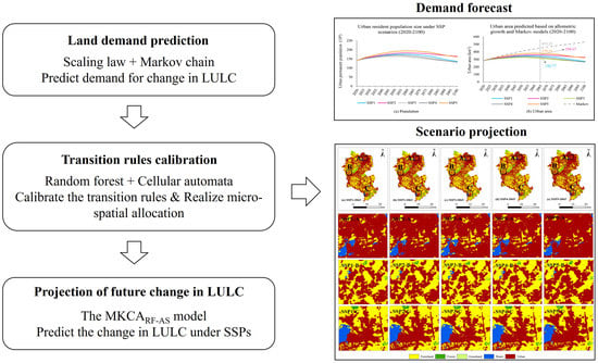
3. Methods
3.1. Calibrating Transition Rules Using Random Forest
3.2. Coupling an Allometric Scaling Law and the Markov Chain to Predict Demand for Change in LULC
3.3. Using Cellular Automata to Allocate Micro-Spatial Changes in LULC
3.4. Scenario Setting
3.5. Method for Evaluating Accuracy
4. Simulation Results
4.1. Land-Use Suitability
4.2. Simulation of Spatial Distribution of LULC
4.3. Sensitivity Analysis
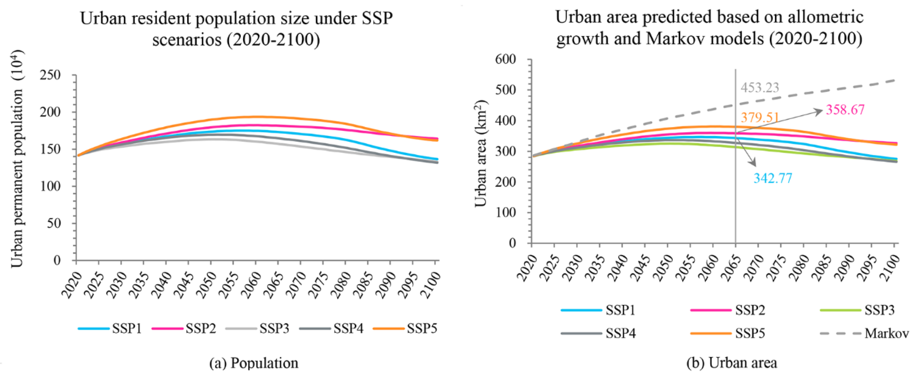
4.4. Allometric Relations between Population Size and Urban Area
4.5. Predicting Urban Land-Use Demand for 2020–2100
4.6. Spatiotemporal Evolution of LULC from 2020 to 2065
4.6.1. Correction of Transition Probability Matrix
4.6.2. Scenario Simulation
4.6.3. Analysis of Urban Expansion on the Township Scale
5. Discussion
6. Conclusions
Author Contributions
Funding
Data Availability Statement
Conflicts of Interest
References
- Beillouin, D.; Cardinael, R.; Berre, D.; Boyer, A.; Corbeels, M.; Fallot, A.; Feder, F.; Demenois, J. A global overview of studies about land management, land-use change, and climate change effects on soil organic carbon. Glob. Chang. Biol. 2022, 28, 1690–1702. [Google Scholar] [CrossRef] [PubMed]
- Ahammad, R.; Hossain, M.K.; Sobhan, I.; Hasan, R.; Biswas, S.R.; Mukul, S.A. Social-ecological and institutional factors affecting forest and landscape restoration in the Chittagong Hill Tracts of Bangladesh. Land Use Policy 2023, 125, 106478. [Google Scholar] [CrossRef]
- De Olivera, L.C.M.; de Mendonça, G.C.; Costa, R.C.A.; de Camargo, R.A.L.; Fernandes, L.F.S.; Pacheco, F.A.L.; Pissarra, T.C.T. Impacts of urban sprawl in the Administrative Region of Ribeirão Preto (Brazil) and measures to restore improved landscapes. Land Use Policy 2023, 124, 106439. [Google Scholar] [CrossRef]
- Sun, Y.; Liu, D.; Wang, P. Urban simulation incorporating coordination relationships of multiple ecosystem services. Sustain. Cities Soc. 2022, 76, 103432. [Google Scholar] [CrossRef]
- Domingo, D.; Van Vliet, J.; Hersperger, A.M. Long-term changes in 3D urban form in four Spanish cities. Landsc. Urban Plan. 2023, 230, 104624. [Google Scholar] [CrossRef]
- Jia, B.; Luo, X.; Wang, L.; Lai, X. Changes in Water Use Efficiency Caused by Climate Change, CO2 Fertilization, and Land Use Changes on the Tibetan Plateau. Adv. Atmos. Sci. 2023, 40, 144–154. [Google Scholar] [CrossRef]
- Black, B.; van Strien, M.J.; Adde, A.; Grêt-Regamey, A. Re-considering the status quo: Improving calibration of land use change models through validation of transition potential predictions. Environ. Model. Softw. 2023, 159, 105574. [Google Scholar] [CrossRef]
- Chen, Y.; Weng, Q.; Tang, L.; Wang, L.; Xing, H.; Liu, Q. Developing an intelligent cloud attention network to support global urban green spaces mapping. ISPRS J. Photogramm. Remote Sens. 2023, 198, 197–209. [Google Scholar] [CrossRef]
- Sun, S.; Parker, D.C.; Brown, D.G. From an agent-based laboratory to the real world: Effects of “neighborhood” size on urban sprawl. Comput. Environ. Urban Syst. 2023, 99, 101889. [Google Scholar] [CrossRef]
- Feng, Y.; Gao, C.; Wang, R.; Li, P.; Xi, M.; Jin, Y.; Tong, X. A moving window-based spatial assessment method for dynamic urban growth simulations. Geocarto Int. 2022, 37, 15282–15301. [Google Scholar] [CrossRef]
- Zhang, B.; Hu, S.; Wang, H.; Zeng, H. A size-adaptive strategy to characterize spatially heterogeneous neighborhood effects in cellular automata simulation of urban growth. Landsc. Urban Plan. 2023, 229, 104604. [Google Scholar] [CrossRef]
- Molinero-Parejo, R.; Aguilera-Benavente, F.; Gómez-Delgado, M.; Shurupov, N. Combining a land parcel cellular automata (LP-CA) model with participatory approaches in the simulation of disruptive future scenarios of urban land use change. Comput. Environ. Urban Syst. 2023, 99, 101895. [Google Scholar] [CrossRef]
- Halder, S.; Das, S.; Basu, S. Use of support vector machine and cellular automata methods to evaluate impact of irrigation project on LULC. Environ. Monit. Assess. 2023, 195, 3. [Google Scholar] [CrossRef] [PubMed]
- Shojaei, H.; Nadi, S.; Shafizadeh-Moghadam, H.; Tayyebi, A.; Van Genderen, J. An efficient built-up land expansion model using a modified U-Net. Int. J. Digit. Earth 2022, 15, 148–163. [Google Scholar] [CrossRef]
- Liu, J.; Xiao, B.; Li, Y.; Wang, X.; Bie, Q.; Jiao, J. Simulation of dynamic urban expansion under ecological constraints using a long short term memory network model and cellular automata. Remote Sens. 2021, 13, 1499. [Google Scholar] [CrossRef]
- Wu, X.; Liu, X.; Zhang, D.; Zhang, J.; He, J.; Xu, X. Simulating mixed land-use change under multi-label concept by integrating a convolutional neural network and cellular automata: A case study of Huizhou, China. GIScience Remote Sens. 2022, 59, 609–632. [Google Scholar] [CrossRef]
- Liang, X.; Guan, Q.; Clarke, K.C.; Liu, S.; Wang, B.; Yao, Y. Understanding the drivers of sustainable land expansion using a patch-generating land use simulation (PLUS) model: A case study in Wuhan, China. Comput. Environ. Urban Syst. 2021, 85, 101569. [Google Scholar] [CrossRef]
- Luo, Z.; Zhang, W.; Wang, Y.; Wang, T.; Liu, G.; Huang, W. Spatial optimization of ecological ditches for non-point source pollutants under urban growth scenarios. Environ. Monit. Assess. 2023, 195, 105. [Google Scholar] [CrossRef]
- Chasia, S.; Olang, L.O.; Sitoki, L. Modelling of land-use/cover change trajectories in a transboundary catchment of the Sio-Malaba-Malakisi Region in East Africa using the CLUE-s model. Ecol. Model. 2023, 476, 110256. [Google Scholar] [CrossRef]
- Lin, X.; Wang, Z. Landscape ecological risk assessment and its driving factors of multi-mountainous city. Ecol. Indic. 2023, 146, 109823. [Google Scholar] [CrossRef]
- Ou, M.; Li, J.; Fan, X.; Gong, J. Compound Optimization of Territorial Spatial Structure and Layout at the City Scale from “Production–Living–Ecological” Perspectives. Int. J. Environ. Res. Public Health 2023, 20, 495. [Google Scholar] [CrossRef]
- Ren, Q.; He, C.; Huang, Q.; Zhang, D.; Shi, P.; Lu, W. Impacts of global urban expansion on natural habitats undermine the 2050 vision for biodiversity. Resour. Conserv. Recycl. 2023, 190, 106834. [Google Scholar] [CrossRef]
- Isinkaralar, O.; Varol, C.; Yilmaz, D. Digital mapping and predicting the urban growth: Integrating scenarios into cellular automata—Markov chain modeling. Appl. Geomat. 2022, 14, 695–705. [Google Scholar] [CrossRef]
- Ouyang, X.; Xu, J.; Li, J.; Wei, X.; Li, Y. Land space optimization of urban-agriculture-ecological functions in the Changsha-Zhuzhou-Xiangtan Urban Agglomeration, China. Land Use Policy 2022, 117, 106112. [Google Scholar] [CrossRef]
- Yang, J.; Tang, W.; Gong, J.; Shi, R.; Zheng, M.; Dai, Y. Simulating urban expansion using cellular automata model with spatiotemporally explicit representation of urban demand. Landsc. Urban Plan. 2023, 231, 104640. [Google Scholar] [CrossRef]
- Overmars, K.P.; De Koning, G.H.J.; Veldkamp, A. Spatial autocorrelation in multi-scale land use models. Ecol. Model. 2003, 164, 257–270. [Google Scholar] [CrossRef]
- Arsanjani, J.J.; Helbich, M.; Kainz, W.; Boloorani, A.D. Integration of logistic regression, Markov chain and cellular automata models to simulate urban expansion. Int. J. Appl. Earth Obs. Geoinf. 2013, 21, 265–275. [Google Scholar] [CrossRef]
- Isinkaralar, O.; Varol, C. A cellular automata-based approach for spatio-temporal modeling of the city center as a complex system: The case of Kastamonu, Türkiye. Cities 2023, 132, 104073. [Google Scholar] [CrossRef]
- Van Vliet, J.; Naus, N.; Van Lammeren, R.J.; Bregt, A.K.; Hurkens, J.; Van Delden, H. Measuring the neighbourhood effect to calibrate land use models. Comput. Environ. Urban Syst. 2013, 41, 55–64. [Google Scholar] [CrossRef]
- Liao, J.; Tang, L.; Shao, G. Multi-Scenario Simulation to Predict Ecological Risk Posed by Urban Sprawl with Spontaneous Growth: A Case Study of Quanzhou. Int. J. Environ. Res. Public Health 2022, 19, 15358. [Google Scholar] [CrossRef]
- Zhang, S.; Zhong, Q.; Cheng, D.; Xu, C.; Chang, Y.; Lin, Y.; Li, B. Landscape ecological risk projection based on the PLUS model under the localized shared socioeconomic pathways in the Fujian Delta region. Ecol. Indic. 2022, 136, 108642. [Google Scholar] [CrossRef]
- Cao, W.; Dong, L.; Cheng, Y.; Wu, L.; Guo, Q.; Liu, Y. Constructing multi-level urban clusters based on population distributions and interactions. Comput. Environ. Urban Syst. 2023, 99, 101897. [Google Scholar] [CrossRef]
- Aretouyap, Z.; Abdelfattah, M.; Gaber, A. Urban sprawl analysis and shoreline extraction in Douala-Cameroon city using optical and radar sensors. Geocarto Int. 2022, 37, 14596–14608. [Google Scholar] [CrossRef]
- Wang, H.; Guo, F. City-level socioeconomic divergence, air pollution differentials and internal migration in China: Migrants vs talent migrants. Cities 2023, 133, 104116. [Google Scholar] [CrossRef]
- Yang, L.; Guo, J.; Cao, S. What structural factors have held back China’s birth rate? Environ. Dev. Sustain. 2022, 1–14. [Google Scholar] [CrossRef]
- Longley, P.A.; Batty, M.; Shepherd, J. The size, shape and dimension of urban settlements. Trans. Inst. Br. Geogr. 1991, 16, 75. [Google Scholar] [CrossRef]
- Kaufmann, T.; Radaelli, L.; Bettencourt, L.M.; Shmueli, E. Scaling of urban amenities: Generative statistics and implications for urban planning. EPJ Data Sci. 2022, 11, 50. [Google Scholar] [CrossRef]
- Abdulrasheed, M.; MacKenzie, A.R.; Whyatt, J.; Chapman, L. Allometric scaling of thermal infrared emitted from UK cities and its relation to urban form. City Environ. Interact. 2020, 5, 100037. [Google Scholar] [CrossRef]
- Lei, W.; Jiao, L.; Xu, G. Understanding the urban scaling of urban land with an internal structure view to characterize China’s urbanization. Land Use Policy 2022, 112, 105781. [Google Scholar] [CrossRef]
- Chen, Y. Multi-scaling allometric analysis for urban and regional development. Phys. A Stat. Mech. Appl. 2017, 465, 673–689. [Google Scholar] [CrossRef]
- Woldenberg, M.J. An allometric analysis of urban land use in the United States. Ekistics 1973, 36, 282–290. [Google Scholar]
- Dutton, G. Criteria of growth in urban systems. Ekistics 1973, 36, 298–306. [Google Scholar]
- Wang, X.; Meng, X.; Long, Y. Projecting 1 km-grid population distributions from 2020 to 2100 globally under shared socioeconomic pathways. Sci. Data 2022, 9, 563. [Google Scholar] [CrossRef] [PubMed]
- Li, Z.; Murshed, M.; Yan, P. Driving force analysis and prediction of ecological footprint in urban agglomeration based on extended STIRPAT model and shared socioeconomic pathways (SSPs). J. Clean. Prod. 2023, 383, 135424. [Google Scholar] [CrossRef]
- JCSB. Bulletin of the Seventh National Population Census of Jinjiang City. 2021. Available online: http://www.jinjiang.gov.cn/xxgk/zfxxgkzl/bmzfxxgk/tjj/zfxxgkml/202105/t20210531_2565668.htm (accessed on 8 January 2023).
- JCSB—Jinjiang City Statistics Bureau and National Bureau of Statistics of China. Jinjiang Statistical Yearbook in 2022; China Statistics Press: Beijing, China, 2022. [Google Scholar]
- Jiang, T.; Su, B.; Wang, Y.; Wang, G.; Luo, Y.; Zhai, J.Q.; Huang, J.; Jing, C.; Gao, M.; Lin, Q. Gridded datasets for population and economy under Shared Socioeconomic Pathways for 2020–2100. Adv. Clim. Chang. Res. 2022, 18, 381–383. [Google Scholar]
- Yang, J.; Huang, X. The 30 m annual land cover dataset and its dynamics in China from 1990 to 2019. Earth Syst. Sci. Data 2021, 13, 3907–3925. [Google Scholar] [CrossRef]
- Breiman, L. Random forests. Mach. Learn. 2001, 45, 5–32. [Google Scholar] [CrossRef]
- Ren, L.; Seklouli, A.S.; Zhang, H.; Wang, T.; Bouras, A. An adaptive Laplacian weight random forest imputation for imbalance and mixed-type data. Inf. Syst. 2023, 111, 102122. [Google Scholar] [CrossRef]
- Pan, Y.; Kong, X.; Yuan, Y.; Sun, Y.; Han, X.; Yang, H.; Zhang, J.; Liu, X.; Gao, P.; Li, Y. Detecting the foreign matter defect in lithium-ion batteries based on battery pilot manufacturing line data analyses. Energy 2023, 262, 125502. [Google Scholar] [CrossRef]
- Wu, J.; Zhao, R.; Sun, J. State transition of carbon emission efficiency in China: Empirical analysis based on three-stage SBM and Markov chain models. Environ. Sci. Pollut. Res. 2023, 1–11. [Google Scholar] [CrossRef]
- Girma, R.; Fürst, C.; Moges, A. Land use land cover change modeling by integrating artificial neural network with cellular Automata-Markov chain model in Gidabo river basin, main Ethiopian rift. Environ. Chall. 2022, 6, 100419. [Google Scholar] [CrossRef]
- Bettencourt, L.M. The origins of scaling in cities. Science 2013, 340, 1438–1441. [Google Scholar] [CrossRef] [PubMed]
- Chen, Y. Scaling, fractals and the spatial complexity of cities. In Handbook on Cities and Complexity; Edward Elgar Publishing: Cheltenham, UK, 2021. [Google Scholar]
- Feng, Y.; Wang, R.; Tong, X.; Zhai, S. Comparison of change and static state as the dependent variable for modeling urban growth. Geocarto Int. 2022, 37, 6975–6998. [Google Scholar] [CrossRef]
- Wang, H.; Guo, J.; Zhang, B.; Zeng, H. Simulating urban land growth by incorporating historical information into a cellular automata model. Landsc. Urban Plan. 2021, 214, 104168. [Google Scholar] [CrossRef]
- Lin, J.; Li, X.; Wen, Y.; He, P. Modeling urban land-use changes using a landscape-driven patch-based cellular automaton (LP-CA). Cities 2023, 132, 103906. [Google Scholar] [CrossRef]
- White, R.; Engelen, G. Cellular automata and fractal urban form: A cellular modelling approach to the evolution of urban land-use patterns. Environ. Plan. A 1993, 25, 1175–1199. [Google Scholar] [CrossRef]
- Zeng, Y.; Hesketh, T. The effects of China’s universal two-child policy. Lancet 2016, 388, 1930–1938. [Google Scholar] [CrossRef]
- Pontius, R.G.; Boersma, W.; Castella, J.-C.; Clarke, K.; de Nijs, T.; Dietzel, C.; Duan, Z.; Fotsing, E.; Goldstein, N.; Kok, K. Comparing the input, output, and validation maps for several models of land change. Ann. Reg. Sci. 2008, 42, 11–37. [Google Scholar] [CrossRef]
- Liu, X.; Liang, X.; Li, X.; Xu, X.; Ou, J.; Chen, Y.; Li, S.; Wang, S.; Pei, F. A future land use simulation model (FLUS) for simulating multiple land use scenarios by coupling human and natural effects. Landsc. Urban Plan. 2017, 168, 94–116. [Google Scholar] [CrossRef]
- Xu, T.; Gao, J.; Coco, G. Simulation of urban expansion via integrating artificial neural network with Markov chain–cellular automata. Int. J. Geogr. Inf. Sci. 2019, 33, 1960–1983. [Google Scholar] [CrossRef]
- Feng, Y.; Liu, Y.; Tong, X.; Liu, M.; Deng, S. Modeling dynamic urban growth using cellular automata and particle swarm optimization rules. Landsc. Urban Plan. 2011, 102, 188–196. [Google Scholar] [CrossRef]
- Nordbeck, S. Urban allometric growth. Geogr. Ann. Ser. B Hum. Geogr. 1971, 53, 54–67. [Google Scholar] [CrossRef]
- Lee, Y. An allometric analysis of the US urban system: 1960–80. Environ. Plan. A 1989, 21, 463–476. [Google Scholar] [CrossRef] [PubMed]
- Chen, Y.; Feng, J. A hierarchical allometric scaling analysis of Chinese cities: 1991–2014. Discret. Dyn. Nat. Soc. 2017, 2017, 5243287. [Google Scholar] [CrossRef]
- Bettencourt, L.M.; Lobo, J.; Helbing, D.; Kühnert, C.; West, G.B. Growth, innovation, scaling, and the pace of life in cities. Proc. Natl. Acad. Sci. USA 2007, 104, 7301–7306. [Google Scholar] [CrossRef]
- Lynch, M.; Trickovic, B.; Kempes, C.P. Evolutionary scaling of maximum growth rate with organism size. Sci. Rep. 2022, 12, 22586. [Google Scholar] [CrossRef]
- Jia, Y.; Tang, L.; Zhang, P.; Xu, M.; Luo, L.; Zhang, Q. Exploring the scaling relations between urban spatial form and infrastructure. Int. J. Sustain. Dev. World Ecol. 2022, 29, 665–675. [Google Scholar] [CrossRef]
- Veregin, H.; Tobler, W.R. Allometric relationships in the structure of street-level databases. Comput. Environ. Urban Syst. 1997, 21, 277–290. [Google Scholar] [CrossRef]
- Lv, M.; Chen, Z.; Yao, L.; Dang, X.; Li, P.; Cao, X. Potential Zoning of Construction Land Consolidation in the Loess Plateau Based on the Evolution of Human–Land Relationship. Int. J. Environ. Res. Public Health 2022, 19, 14927. [Google Scholar] [CrossRef]
- Chen, Y. An extended patch-based cellular automaton to simulate horizontal and vertical urban growth under the shared socioeconomic pathways. Comput. Environ. Urban Syst. 2022, 91, 101727. [Google Scholar] [CrossRef]
- Xiong, Y.; Jiao, G.; Zheng, J.; Gao, J.; Xue, Y.; Tian, B.; Cheng, J. Fertility Intention and Influencing Factors for Having a Second Child among Floating Women of Childbearing Age. Int. J. Environ. Res. Public Health 2022, 19, 16531. [Google Scholar] [CrossRef] [PubMed]
- QWCB—Quanzhou Water Conservancy Bureau. Quanzhou Water Resources Bulletin in 2020. 2020. Available online: http://slj.quanzhou.gov.cn/zwgk/tzgg/202111/t20211119_2655072.htm (accessed on 6 April 2023).
- Chen, Y.; Li, X.; Liu, X.; Zhang, Y.; Huang, M. Quantifying the teleconnections between local consumption and domestic land uses in China. Landsc. Urban Plan. 2019, 187, 60–69. [Google Scholar] [CrossRef]
- Oppenheimer, M.; Glavovic, B.; Hinkel, J.; van de Wal, R.; Magnan, A.K.; Abd-Elgawad, A.; Cai, R.; Cifuentes-Jara, M.; Deconto, R.M.; Ghosh, T. Sea level rise and implications for low lying islands, coasts and communities. In IPCC Special Report on the Ocean and Cryosphere in a Changing Climate. 2019. Available online: https://www.ipcc.ch/srocc/chapter/chapter-4-sea-level-rise-and-implications-for-low-lying-islands-coasts-and-communities/ (accessed on 15 April 2023).


| Changes in Demand for Urban Land Use | 2005–2010 | 2005–2015 | 2005–2020 | ||||||
|---|---|---|---|---|---|---|---|---|---|
| Urban Land (Cells) | FoM (%) | Urban FoM (%) | Urban Land (Cells) | FoM (%) | Urban FoM (%) | Urban Land (Cells) | FoM (%) | Urban FoM (%) | |
| Predicted change in land use by Markov model | 244,954 | 23.45 | 27.52 | 263,221 | 27.21 | 32.40 | 277,949 | 21.37 | 27.76 |
| +2% | 249,853 | 24.31 | 29.95 | 268,485 | 27.46 | 33.74 | 283,508 | 21.48 | 28.55 |
| +2% | 254,752 | 24.78 | 32.05 | 273,750 | 27.75 | 35.11 | 289,067 | 21.57 | 29.31 |
| +2% | 279,014 | 28.00 | 36.43 | 294,626 | 21.76 | 30.18 | |||
| +2% | 284,279 | 28.19 | 37.63 | 300,185 | 21.96 | 31.13 | |||
| +2% | 305,744 | 21.97 | 31.85 | ||||||
| +2% | 311,303 | 22.21 | 32.79 | ||||||
| Actual demand for urban land use | 261,381 | 25.48 | 35.02 | 292,024 | 28.27 | 39.24 | 318,210 | 22.21 | 33.68 |
| Year | 2005 | 2006 | 2007 | 2008 | 2009 | 2010 | 2011 | 2012 | 2013 | 2014 | 2015 | 2016 | 2017 | 2018 | 2019 | 2020 |
|---|---|---|---|---|---|---|---|---|---|---|---|---|---|---|---|---|
| POP | 67.7 | 72.2 | 74.0 | 76.7 | 80.9 | 117.3 | 120.7 | 124.9 | 128.4 | 132.2 | 133.5 | 135.8 | 139.0 | 141.4 | 142.8 | 141.6 |
| POP-SSNPC | 94.8 | 101.1 | 103.5 | 107.4 | 113.3 | 117.3 | 118.5 | 122.7 | 126.1 | 129.8 | 131.1 | 133.4 | 136.5 | 138.9 | 140.3 | 141.6 |
| UBA | 200.4 | 207.7 | 213.7 | 218.7 | 228.4 | 235.6 | 241.4 | 246.8 | 253.4 | 259.6 | 263.2 | 267.9 | 274.9 | 281.2 | 285.6 | 286.4 |
| UBA-AS | 195.7 | 207.7 | 212.4 | 219.8 | 231.1 | 238.6 | 241.0 | 249.0 | 255.4 | 262.4 | 264.9 | 269.0 | 275.0 | 279.5 | 282.0 | 284.6 |
| SPP Scenarios | Probability of Shifting to the Following Land-Use Type | ||||
|---|---|---|---|---|---|
| Agricultural | Woodland | Grassland | Water | Built-Up | |
| 2005–2020 | |||||
| Agricultural | 0.7829 | 0.0166 | 0.0018 | 0.0039 | 0.1948 |
| Woodland | 0.3092 | 0.6653 | 0.0005 | 0.0001 | 0.0249 |
| Grassland | 0.3487 | 0.0068 | 0.0327 | 0.0088 | 0.6031 |
| Water | 0.2218 | 0.0004 | 0.0024 | 0.5193 | 0.2561 |
| Built-up | 0.0004 | 0.0000 | 0.0000 | 0.0025 | 0.9971 |
| 2020–2065 (SSP1) | |||||
| Agricultural | 0.9132 | 0.0211 | 0.0021 | 0.0051 | 0.0585 |
| Woodland | 0.2895 | 0.6989 | 0.0004 | 0.0000 | 0.0114 |
| Grassland | 0.7454 | 0.0161 | 0.0476 | 0.0306 | 0.1606 |
| Water | 0.2870 | 0.0002 | 0.0030 | 0.6366 | 0.0733 |
| Built-up | 0.0002 | 0.0000 | 0.0000 | 0.0022 | 0.9976 |
| 2020–2065 (SSP2) | |||||
| Agricultural | 0.8966 | 0.0206 | 0.0021 | 0.0050 | 0.0757 |
| Woodland | 0.2913 | 0.6943 | 0.0004 | 0.0000 | 0.0142 |
| Grassland | 0.7043 | 0.0150 | 0.0409 | 0.0287 | 0.2114 |
| Water | 0.2793 | 0.0003 | 0.0029 | 0.6223 | 0.0953 |
| Built-up | 0.0002 | 0.0000 | 0.0000 | 0.0022 | 0.9975 |
| 2020–2065 (SSP5) | |||||
| Agricultural | 0.8740 | 0.0198 | 0.0021 | 0.0048 | 0.0994 |
| Woodland | 0.2941 | 0.6881 | 0.0004 | 0.0000 | 0.0175 |
| Grassland | 0.6402 | 0.0133 | 0.0385 | 0.0257 | 0.2826 |
| Water | 0.2685 | 0.0003 | 0.0027 | 0.6025 | 0.1260 |
| Built-up | 0.0003 | 0.0000 | 0.0000 | 0.0023 | 0.9975 |
| Land-Use Types | 2020 | 2065 (SSP1) | 2020–2065 (SSP1) | 2065 (SSP2) | 2020–2065 (SSP2) | 2065 (SSP3) | 2020–2065 (SSP3) | 2065 (SSP4) | 2020–2065 (SSP4) | 2065 (SSP5) | 2020–2065 (SSP5) |
|---|---|---|---|---|---|---|---|---|---|---|---|
| Area (km2) | Area (km2) | % | Area (km2) | % | Area (km2) | % | Area (km2) | % | Area (km2) | % | |
| Agricultural | 331.36 | 281.47 | −15.05 | 266.72 | −19.51 | 308.92 | −6.77 | 296.15 | −10.62 | 247.78 | −25.22 |
| Woodland | 25.44 | 23.23 | −8.67 | 22.39 | −11.99 | 24.83 | −2.40 | 24.03 | −5.54 | 21.51 | −15.44 |
| Grassland | 0.92 | 0.70 | −23.90 | 0.68 | −26.63 | 0.80 | −12.78 | 0.74 | −19.71 | 0.65 | −29.56 |
| Water | 11.84 | 8.36 | −29.37 | 8.18 | −30.87 | 9.10 | −23.12 | 8.70 | −26.49 | 7.84 | −33.80 |
| Built-up | 286.39 | 342.63 | 19.64 | 358.43 | 25.16 | 312.94 | 9.27 | 326.89 | 14.14 | 378.92 | 32.31 |
Disclaimer/Publisher’s Note: The statements, opinions and data contained in all publications are solely those of the individual author(s) and contributor(s) and not of MDPI and/or the editor(s). MDPI and/or the editor(s) disclaim responsibility for any injury to people or property resulting from any ideas, methods, instructions or products referred to in the content. |
© 2023 by the authors. Licensee MDPI, Basel, Switzerland. This article is an open access article distributed under the terms and conditions of the Creative Commons Attribution (CC BY) license (https://creativecommons.org/licenses/by/4.0/).
Share and Cite
Liao, J.; Tang, L.; Shao, G. Coupling Random Forest, Allometric Scaling, and Cellular Automata to Predict the Evolution of LULC under Various Shared Socioeconomic Pathways. Remote Sens. 2023, 15, 2142. https://doi.org/10.3390/rs15082142
Liao J, Tang L, Shao G. Coupling Random Forest, Allometric Scaling, and Cellular Automata to Predict the Evolution of LULC under Various Shared Socioeconomic Pathways. Remote Sensing. 2023; 15(8):2142. https://doi.org/10.3390/rs15082142
Chicago/Turabian StyleLiao, Jiangfu, Lina Tang, and Guofan Shao. 2023. "Coupling Random Forest, Allometric Scaling, and Cellular Automata to Predict the Evolution of LULC under Various Shared Socioeconomic Pathways" Remote Sensing 15, no. 8: 2142. https://doi.org/10.3390/rs15082142