Communication

Time Ring Data: Definition and Application in Spatio-Temporal Analysis of Urban Expansion and Forest Loss

School of Spatial Planning and Design, Hangzhou City University, Hangzhou 310015, China
*
Author to whom correspondence should be addressed.
Remote Sens. 2023, 15(4), 972; https://doi.org/10.3390/rs15040972
Submission received: 11 November 2022 / Revised: 13 January 2023 / Accepted: 8 February 2023 / Published: 10 February 2023
(This article belongs to the Special Issue Remote Sensing and GIS for Monitoring Urbanization and Urban Health)

Abstract

:
Remote sensing can provide spatio-temporal continuous Earth observation data and is becoming the main data source for spatial and temporal analysis. Remote sensing data have been widely used in applications such as meteorological monitoring, forest investigation, environmental health, urban planning, and water conservancy. While long-time-series remote sensing data are used for spatio-temporal analysis, this analysis is usually limited because of the large data volumes and complex models used. This study intends to develop an innovative and simple approach to reveal the spatio-temporal characteristics of geographic features from the perspective of remote sensing data themselves. We defined an efficient remote sensing data structure, namely time ring (TR) data, to depict the spatio-temporal dynamics of two common geographic features. One is spatially expansive features. Taking nighttime light (NTL) as an example, we generated a NTL TR map to exhibit urban expansion with spatial and temporal information. The speed and acceleration maps of NTL TR data indicated extraordinary expansion in the last 10 years, especially in coastal cities and provincial capitals. Beijing, Tianjin, Hebei Province, Shandong Province, and Jiangsu Province exhibited fast acceleration of urbanization. The other is spatially contractive features. We took forest loss in the Amazon basin as an example and produced a forest cover TR map. The speed and acceleration were mapped in two 10-year periods (2000–2010 and 2010–2020) in order to observe the changes in Amazon forest cover. Then, combining cropland TR data, we determined the consistency of the spatio-temporal variations and used a linear regression model to detect the association between the acceleration of cropland and forest. The forest TR map showed that, spatially, there was an apparent phenomenon of forest loss occurring in the southern and eastern Amazon basin. Temporally, the speed of forest loss was more drastic between 2000 and 2010 than that in 2010–2020. In addition, the acceleration of forest loss showed a dispersed distribution, except for in Bolivia, which demonstrated a concentrated regional acceleration. The R-squared value of the linear regression between forest and cropland acceleration reached 0.75, indicating that forest loss was closely linked to the expansion of cropland. The TR data defined in this study not only optimized the use of remote sensing data, but also facilitated their application in spatio-temporal integrative analysis. More importantly, multi-field TR data could be jointly applied to explore the driving force at spatial and temporal scales.

Graphical Abstract

1. Introduction

Spatial and temporal variation analysis of geographic features is an important part of geographic research that helps us to understand the characteristics of geographic features [1]. Furthermore, we can predict the potential variations in such characteristics so as to assess the rationality of the variations and the possible risks, and put forward corresponding countermeasures. At present, the data sources for spatio-temporal variation analysis are usually divided into ground observation data and remote sensing (RS) data [2]. With the development of RS techniques, satellite RS images have gradually become the main data source because they can provide spatio-temporal continuous Earth observations [3]. RS data, to date, have been widely used in applications such as meteorological monitoring, forest investigation, environmental health, urban planning, water conservancy, and global climate change [4,5,6,7,8,9].
However, remote sensing data may be a burden when performing long-time-series and large-geographical-scale research [10,11]. These studies involve massive amounts of data, forcing researchers to perform additional data organization work to conduct spatio-temporal change detection analysis [12]. For specific geographic features with the characteristics of a large covered range and long time series, such as flood expansion [13], urban expansion [14], and forest cover change monitoring [15], remote sensing data need to be pre-processed to fit the model inputs, which is time-consuming and labor-intensive work. A large body of work has been conducted due to the proliferation of RS data. For example, Ma built a data-intensive index to decrease the computing complexity for long-time-span and large-range RS applications [16]. Xu put forward a spatial featured data cube analysis tool conducting time-series RS data processing and analysis based on multidimensional spatio-temporal data models, took Poyang Lake data cube datasets for 20 years as an example, and successfully mapped the percentage change in the water area of Poyang Lake over a 20-year time series [10]. Such methods solved the problem of tedious data processing, but research about RS data processing for spatio-temporal distribution analysis of features is still insufficient.
It Is also essential to take into account appropriate approaches in the spatio-temporal analysis of geographic features [17]. Most studies conducting spatiotemporal analysis of RS data simply involved the cognition of the spatial distribution of features at different times [18,19,20,21]. These studies inherently spatially and temporally separated out difficult-to-mine spatio-temporal integrative information. Furthermore, when involving long-time-series or large-scale analysis, these approaches are unwieldy for understanding spatio-temporal characteristics. At present, there are no studies on how to present spatio-temporal integrative characteristics in practical applications based on long-time-series RS data.
Several studies have utilized an effective data form to store long-term changing features and present the spatial variation with time on one map [22,23,24]. For example, Gong produced one global artificial impervious area (GAIA) map from 1985 to 2018, and this data storage was convenient and the spatial variation in GAIA with time could be clearly understood. However, the GAIA data were used only for mapping, lacking further spatio-temporal dynamic analysis based on the data structure. In addition, similar studies failed to explore the general specification and potential practical value of the data form. Therefore, this study proposed time ring (TR) data from the perspective of remote sensing data organization on the basis of previous studies. The TR data are intended to exhibit the spatial variation in geographic features over time, which can intuitively show the spatio-temporal characteristics of geographic features. The TR data structure that we defined is efficient for two types of features. One is space-expansive features over time, such as urban buildings [14] and nighttime light [25]. The other is space-contractive features over time, such as forest cover [26] and glacier cover [27]. Different processing methods will be performed when producing TR data according to the different types of features.
This study provides a detailed definition of TR data and illustrates the steps involved in transforming multi-temporal RS data into TR data. Then, we introduce related calculations and applications of TR data. Two examples of nighttime light TR data and forest cover TR data are provided to explain the spatio-temporal characteristics. Additionally, we perform an ordinary linear regression analysis combining forest and cropland TR data to reveal the driving mechanism spatially and temporally. Finally, this study discusses the strengths and weaknesses of TR data and states the possible application prospects in the future.

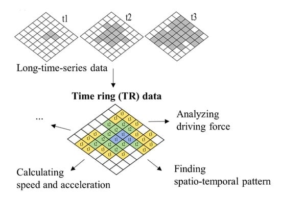
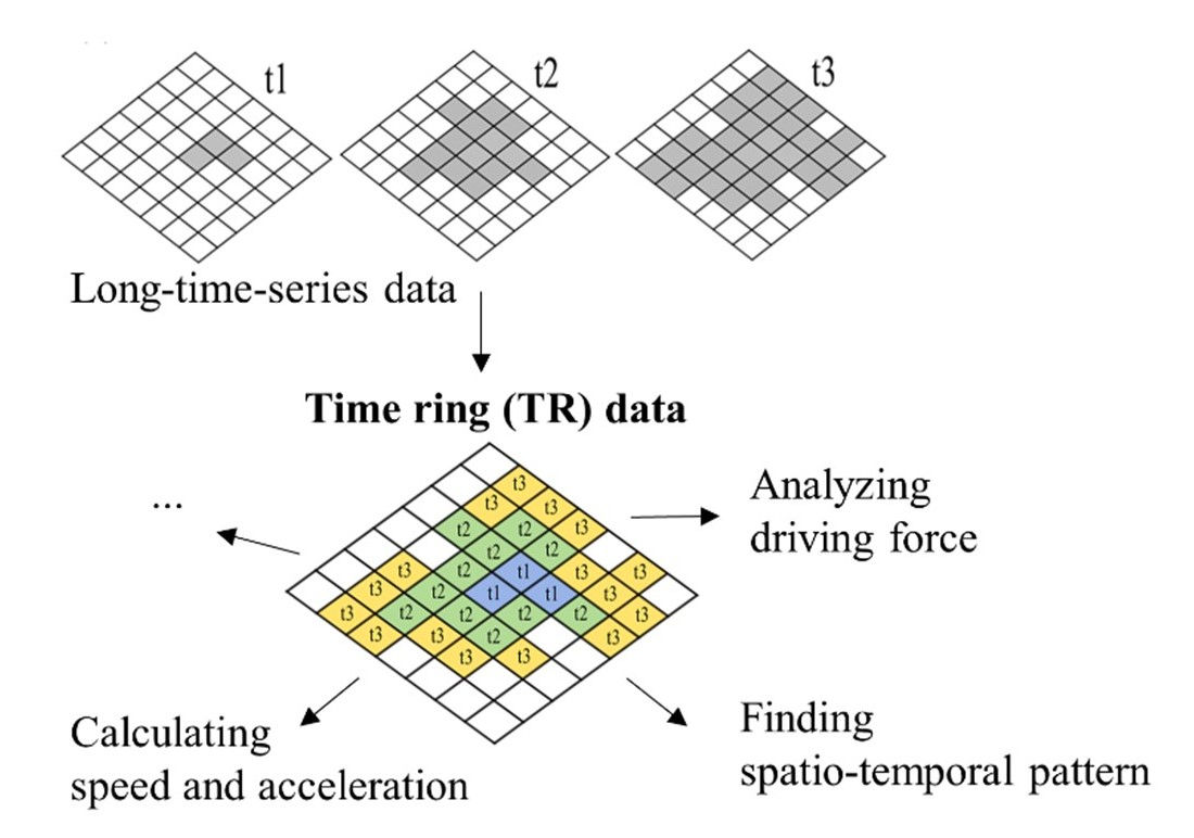
2. Details of Time Ring (TR) Data

2.1. Definition of TR Data

Time ring (TR) data are a new form based on RS data in which geographic features are exhibited like tree rings, which can clearly present the spatial variation characteristics over time (Figure 1). These data rely on long-time-series remote sensing images because a long time series can better show the spatio-temporal variation characteristics of geographic features. Too few time slices may be detrimental to their subsequent exploitation in space and time. The primary trait of TR data for geographic features is either expansive or contractive (Figure 1). For expansive features, the spatial distribution area of these features will gradually increase with temporal change, while for contractive features, the spatial distribution area of these features will gradually decrease with temporal change. The determination of expansion and contraction can be found in Section 2.2. Each grid unit in the TR data is marked by a time label in order to represent integrative temporal and spatial information. The time label denotes when the feature appears or disappears in this grid. For example, for expansive features, such as urban areas, there are different urban areas in t1, t2, and t3. Then, when forming TR data, t2 in each grid indicates that the urban area was emerging in time t2. This expression of data assures that information can be obtained regarding the time at which the spatial changes happened. Furthermore, researchers can perform analysis using a regression model combining multiple TR variables in various fields of application.

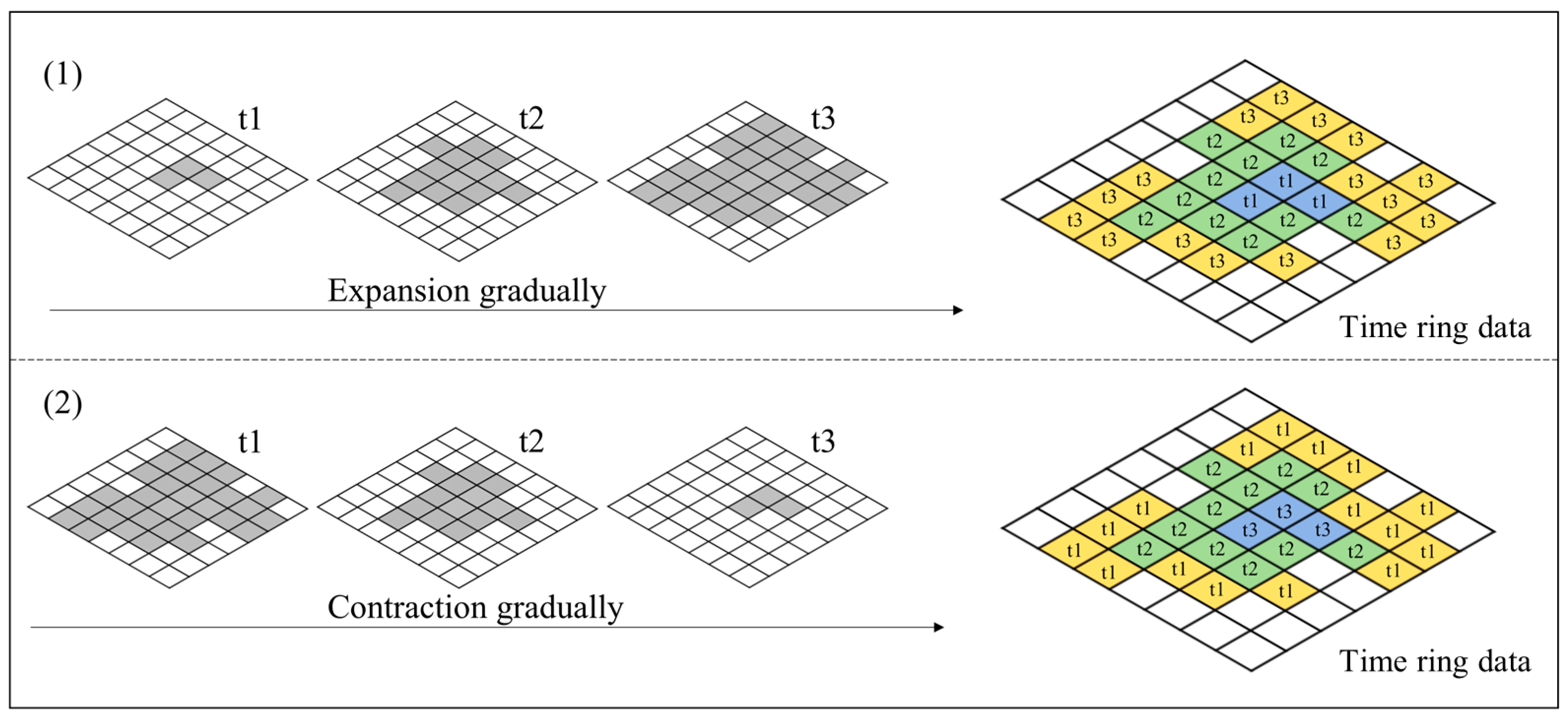
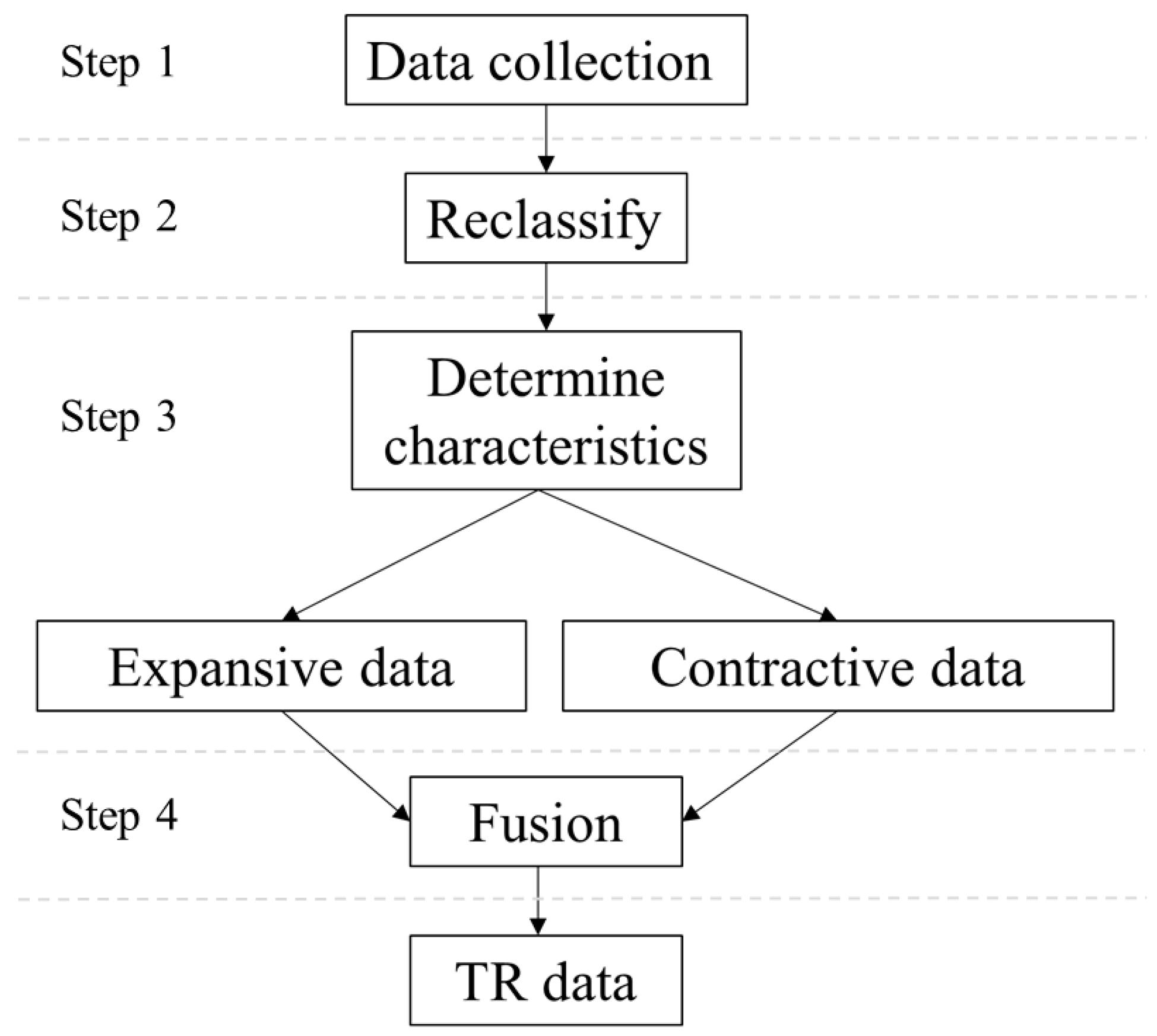
2.2. Generation of TR Data

The generation of TR data involves four steps (Figure 2). The first step is to obtain a relevant remote sensing dataset with notable geographic features. Some datasets can be downloaded based on open-source satellite sensor data, such as normalized differential vegetation index (NDVI) data released by the Moderate-Resolution Imaging Spectroradiometer (MODIS) and nighttime light data produced by the Visible Infrared Imaging Radiometer Suite (VIIRS). Others are subject to further interpretation according to the original image, such as land cover data and urban built-up area data. The second step is to reclassify all images by assigning each pixel of the feature a time label and setting the other pixels to null. The third step is to determine whether the geographic feature is spatially expansive or contractive. We sum up the number of time labels on each image and establish whether the total increased or decreased over time. If the count is increasing, we consider it an expanding feature; otherwise, it is a contracting feature. The last step is to fuse all images in chronological order and produce the TR data. If a feature is expanding outward, the central region represents an older time and the peripheral regions’ time is newer. If a feature is contracting inward, then the central region represents a newer time and the peripheral region time is older.

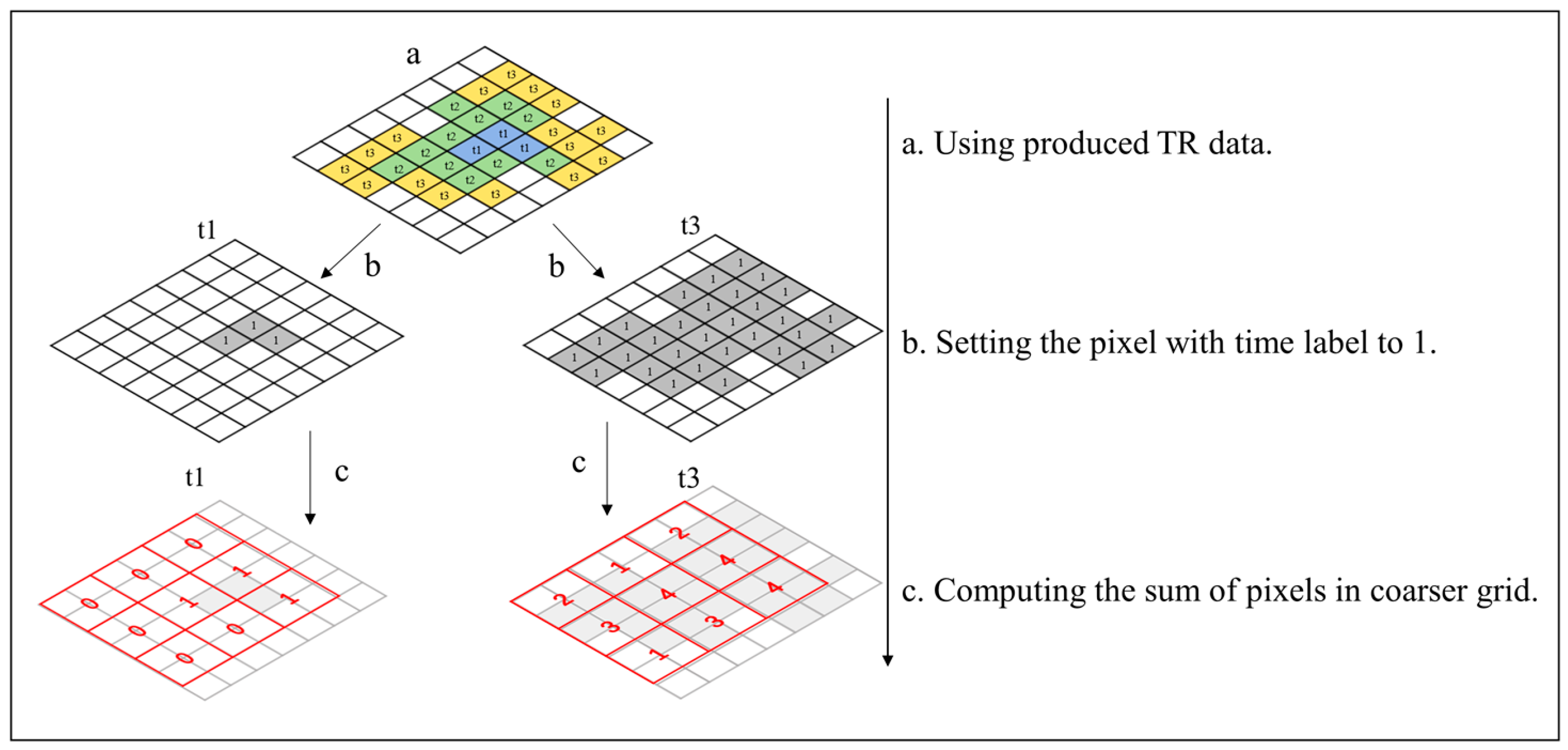
2.3. Calculation of TR Data

Producing TR data is a key step, and the subsequent related analysis will be performed with TR data. In this study, we take into account speed and acceleration as a method of calculating TR data. Speed is used to describe the state of change in features in different periods regarding, specifically, a changing extent of expansion or contraction. Additionally, acceleration is a further calculation based on speed denoting the magnitude of the impact of the driving force [14]. The calculated expression was improved on the basis of our previously published article regarding the analysis of built-up area expansion [14]. Concretely, we first set the pixel with time labels to 1 using produced TR data (Figure 3). Then, we define a fishing net with a coarser resolution (5 × 5 km) than the pixel. The 5 km grid is suitable for larger-scale studies. In practice, we can flexibly set the grid size in terms of spatial scale in the study. The sum of all pixel values in each grid of the fishing net is counted as the grid value (Figure 3). In the end, the grid value is used to compute the speed and acceleration.
In this calculation, speed is defined as the difference in grid value between two time points multiplied by the pixel size and divided by the time interval. Acceleration is defined as the difference in speed between two periods divided by the time interval. The formulae for speed and acceleration are as follows:
S p e e d i , t 0 t 1 = ( a r e a i , t 1 a r e a i , t 0 ) / ( t 1 t 0 )
S p e e d i , t 1 t 2 = ( a r e a i , t 2 a r e a i , t 1 ) / ( t 2 t 1 )
A c c e l e r a t i o n i , T = ( S p e e d i , t 1 t 2 S p e e d i , t 0 t 1 ) / T
where areat0, areat1, and areat2 represent the object areas at time t1, t2, and t3, respectively. i represents each grid defined during data preparation (Figure 3). t0→t1 and t1→t2 represent two periods for calculating their speed. T represents the interval between the two periods for calculating their acceleration. The speed and acceleration are just one form of the calculation of TR data. Subsequent studies will further explore the analysis of TR data based on other methods, such as Moran’s I.

3. Application to Urban Expansion

3.1. Nighttime Light Data

The TR data, on one hand, can be clearly used to recognize the time label when there is a spatial variation. On the other hand, they are able to characterize the driving force by combining other TR data. It is appropriate for use in the analysis of urban expansion under the context of global urbanization. Many studies have discussed the temporal variation and driving force of urban expansion by extracting the build-up area from remote sensing images, such as Landsat and Sentinel images [14,22]. In this study, we attempt to map the nighttime light (NTL) data to exhibit the urban expansion in China in 2000–2020. NTL data with a long time series can be obtained from the website https://dataverse.harvard.edu, accessed on 1 September 2022 [28]. Urban expansion represents a type of geographic feature with spatial expansion. As many studies on the spatial and temporal characteristics of urban expansion have been conducted, further influential mechanisms will not be discussed in this study. However, we produced the speed and acceleration map of NTL TR data to analyze the potential spatio-temporal characteristics.

3.2. Results of Urban Expansion

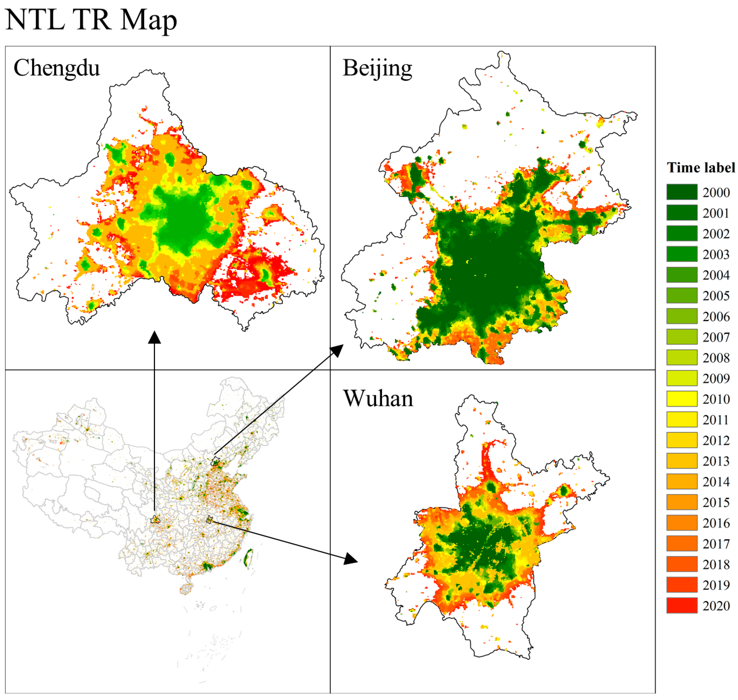
3.2.1. Spatio-Temporal Characteristics of NTL TR Data

According to the generated NTL TR map (Figure 4), comparing the three cities of Chengdu, Wuhan, and Beijing, the result shows that the largest NTL area was in Beijing in 2000, indicating the rapid development of urbanization in this period [29,30], while Chengdu and Wuhan were still in the early stages of development during this period. The NTL TR map also shows that the eastern part of Chengdu has maintained a state of rapid development in recent years. The application of urban expansion may be used to explain some phenomena caused by urban development, such as ecological environmental change.

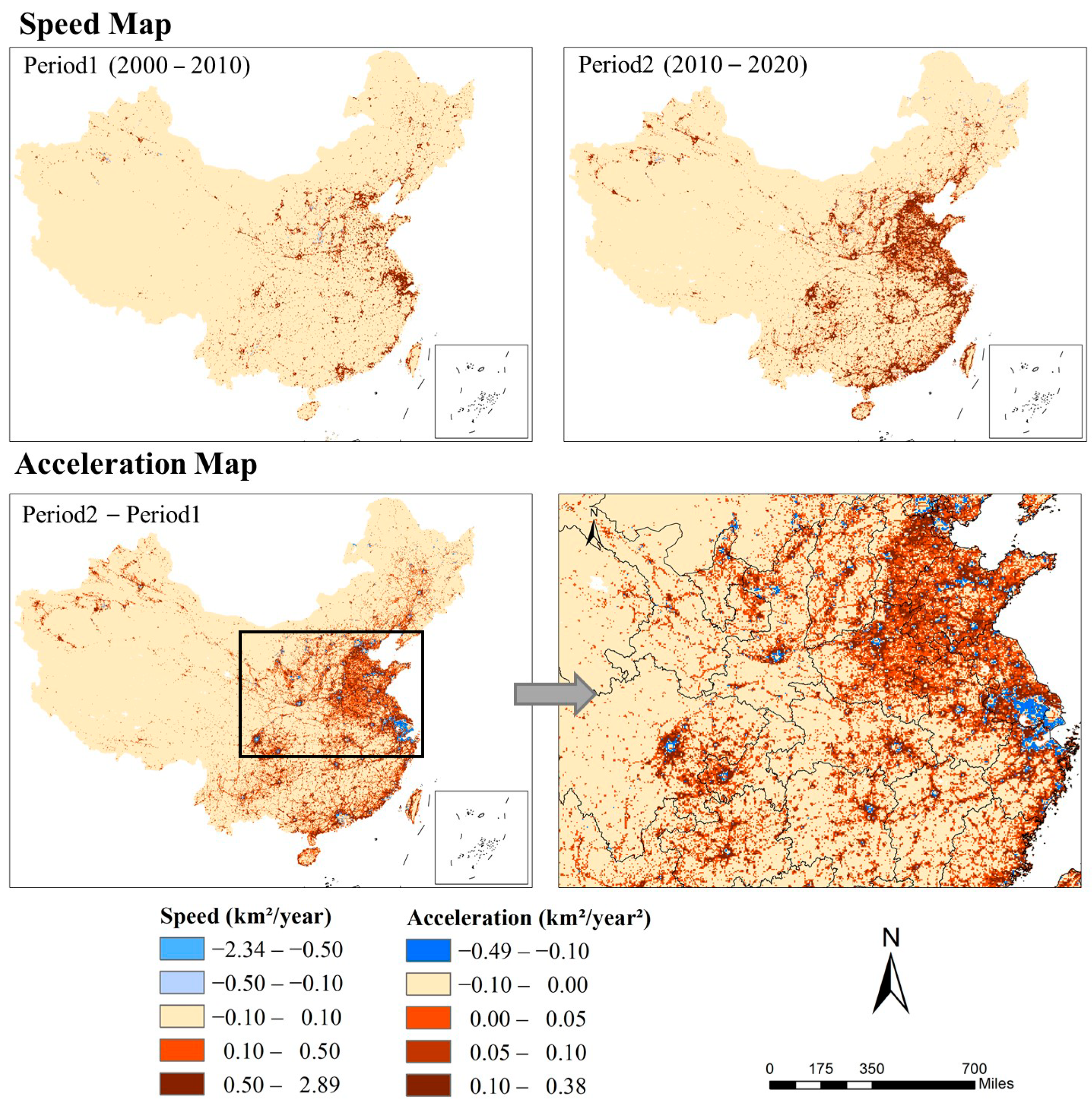
3.2.2. Analysis of Speed and Acceleration of NTL in China

The increase in the NTL area can reflect the urban expansion, while the changing speed and acceleration of the NTL can also indirectly show the expansion rate and acceleration of urban areas. During the two periods (2000–2010 and 2010–2020), from the distribution map of speed and acceleration of NTL in China (Figure 5), we can establish that the overall speed in eastern China has been relatively high since 2000, indicating that these cities have experienced a rapid expansion. In addition, some provincial capitals in the central and western regions, such as Chengdu, Xi’an, and Wuhan, have also experienced significant expansion. In contrast, some cities developed more rapidly in period 2. The acceleration map shows that Beijing, Tianjin, Hebei Province, Shandong Province, and Jiangsu Province exhibited a high acceleration in urbanization. However, there are negative variations in acceleration in the central area of some provincial capitals, indicating that the NTL in the center of these cities is decreasing, which is especially significant around Shanghai.

4. Application to Forest Cover Change

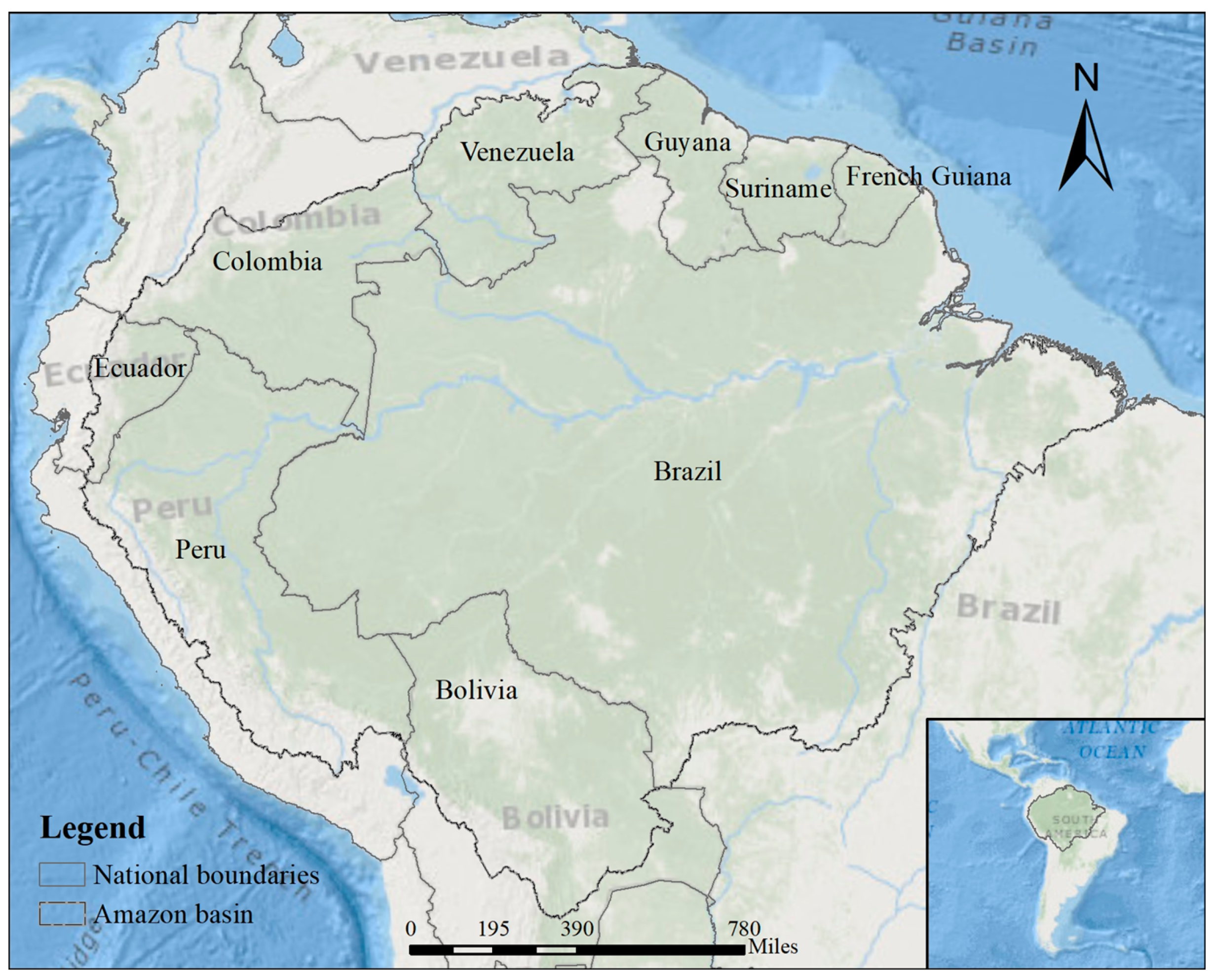
4.1. Study Area and Data

This study takes forest cover data in the Amazon basin as an example to check the utility of the TR data. The Amazon basin covers 7.05 million square kilometers, accounting for 40% of the total area of the South American continent. The region consists of parts of Brazil, Bolivia, Peru, Ecuador, Colombia, Venezuela, Guyana, Suriname, and French Guiana (Figure 6). The region has the largest tropical rainforest in the world, benefitting humankind by purifying the atmosphere and adjusting the climate. However, due to the impact of human activities, such as agricultural expansion, logging, and urban expansion, the land cover in the Amazon basin has undergone dramatic changes, especially with the massive loss of forest [31].
In this case, we screened out the forest and cropland datasets in the Amazon basin from 2000 to 2020 based on global land cover (LC) classification data. The global LC classification data can be obtained from the website https://cds.climate.copernicus.eu (accessed on 7 February 2023), which includes two sources. One is the global annual LC maps from 1992 to 2015 produced by the European Space Agency (ESA) Climate Change Initiative (CCI) LC project [32,33]. The other is the Copernicus Climate Change Service (C3S), which generated global LC maps from 2016 to 2020 that are consistent with the ESA-CCI LC maps. The LC classification data were defined using the United Nations Food and Agriculture Organization’s (UN FAO) Land Cover Classification System (LCCS). The long-time-series LC classification data with a spatial resolution of 300 m are well suited to fine spatio-temporal analysis.
We produced the forest cover TR data in the Amazon basin based on the proposed generation method. Then, we extracted forest cover data from the TR data in 2000, 2010, and 2020 in order to create speed and acceleration maps. Furthermore, we also created a cropland TR map and an acceleration map in the Amazon basin to analyze the driving force of forest cover change, and observed their spatio-temporal variation characteristics based on these two TR maps. At the same time, ordinary linear regression was also utilized to establish the relationship between acceleration changes in forest and cropland.

4.2. Results of Forest Cover Change

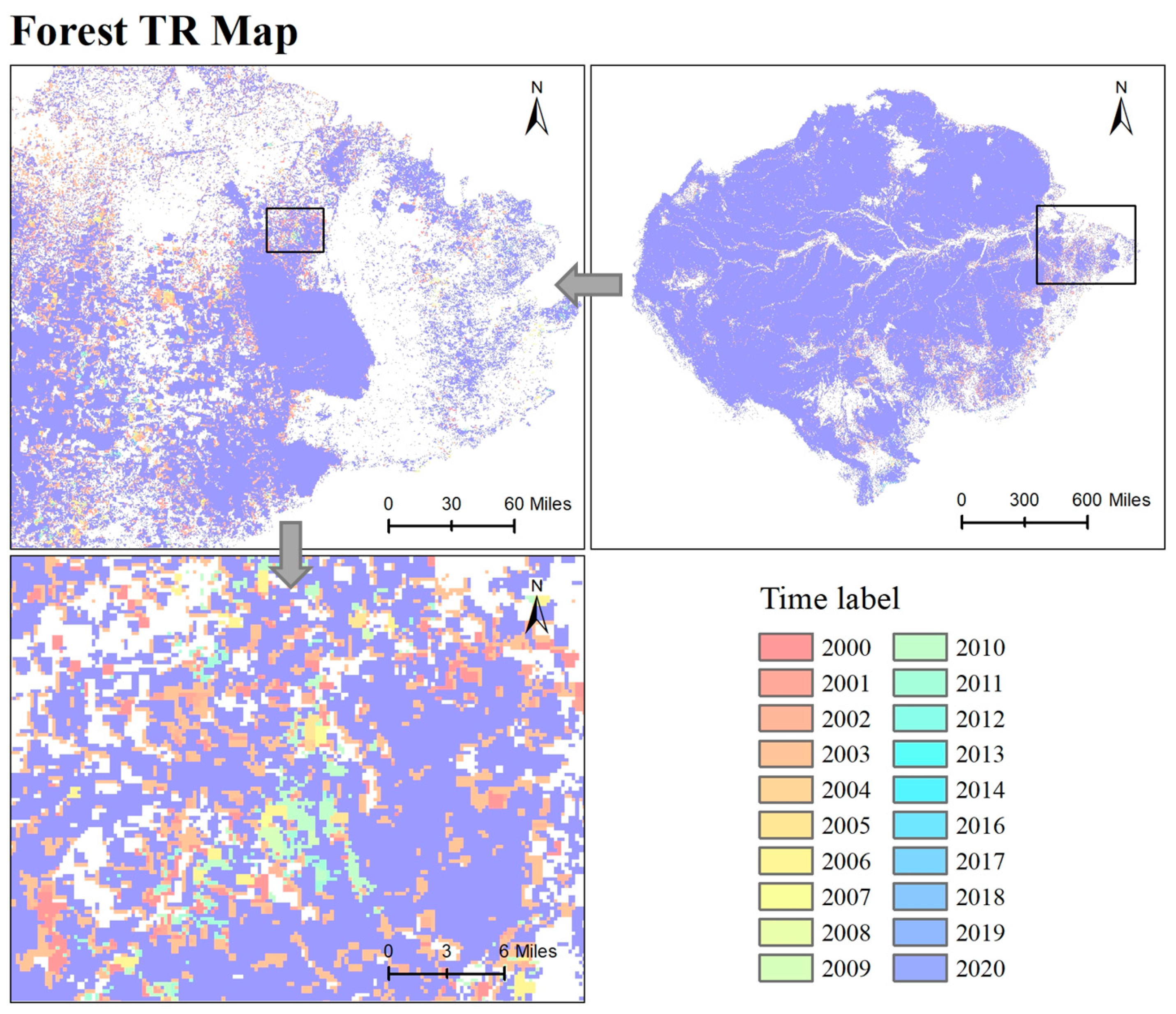
4.2.1. Spatio-Temporal Characteristics of Forest TR Data

We produced TR data based on forest cover from 2000 to 2020 in the Amazon basin (Figure 7). Despite the high level of forest cover in the Amazon basin, there has been significant loss since the beginning of the 21st century. Forest loss is usually a process occurring from the edge to the center at the local scale, so the display of TR data was obvious. Overall, forest loss mostly occurred at the edge of the Amazon basin and near the main river and its tributaries (Figure 7). From a regional perspective, an apparent phenomenon of forest loss occurring in the southern and eastern Amazon basin was observed. According to the mapping result, forest loss in the Amazon basin was most significant between 2000 and 2010.

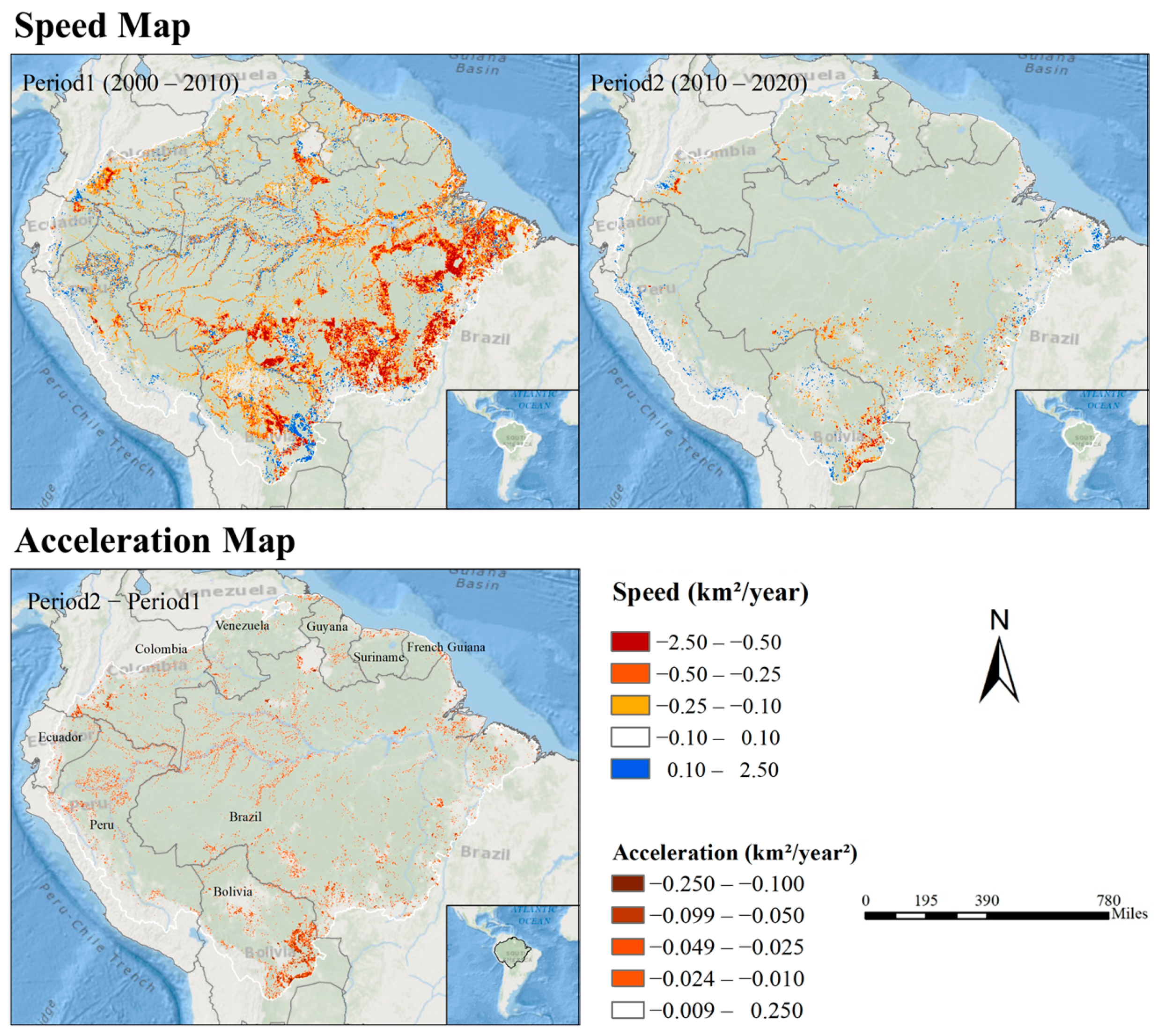
4.2.2. Analysis of Speed and Acceleration

We mapped the speed and acceleration of forest loss for two periods (2000–2010 and 2010–2020) in the Amazon basin (Figure 8). By comparing the variation in speed between these two periods, we found that the speed of forest loss was more drastic in the first period. Spatially, the speed of forest loss was higher in the southeastern Amazon basin, mainly in Brazil, than in other regions. There was also a high speed of forest loss in some local areas, such as Caquetá Province in Colombia and central Bolivia. In the period of 2010–2020, the speed of forest loss slowed down overall, with higher speed only in the southern Amazon basin. From the acceleration map, the regional characteristics of forest loss were not obvious. Only in Bolivia was there a concentrated area of acceleration of forest loss. However, there was an acceleration of forest loss occurring in the whole region of the Amazon basin.

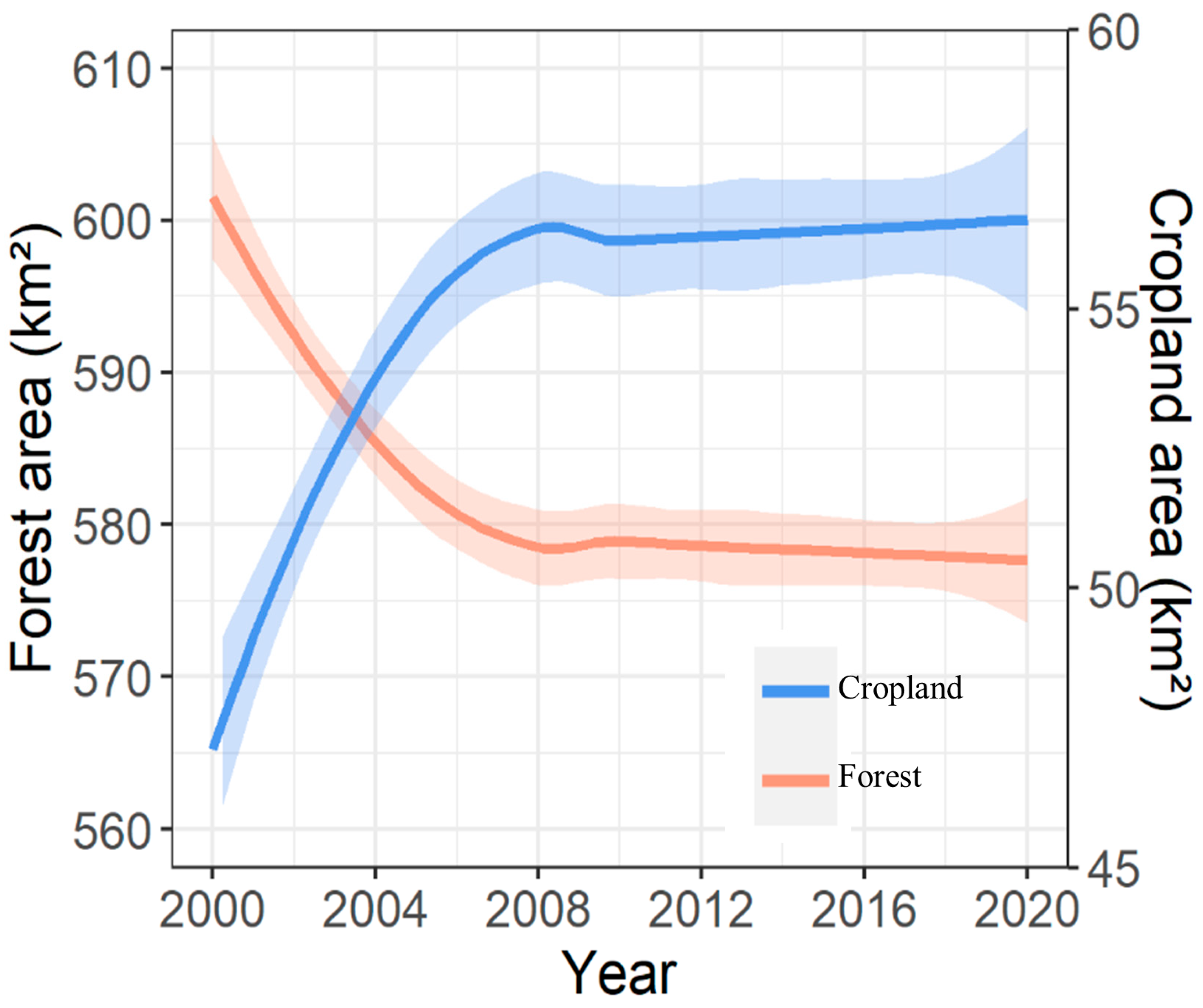
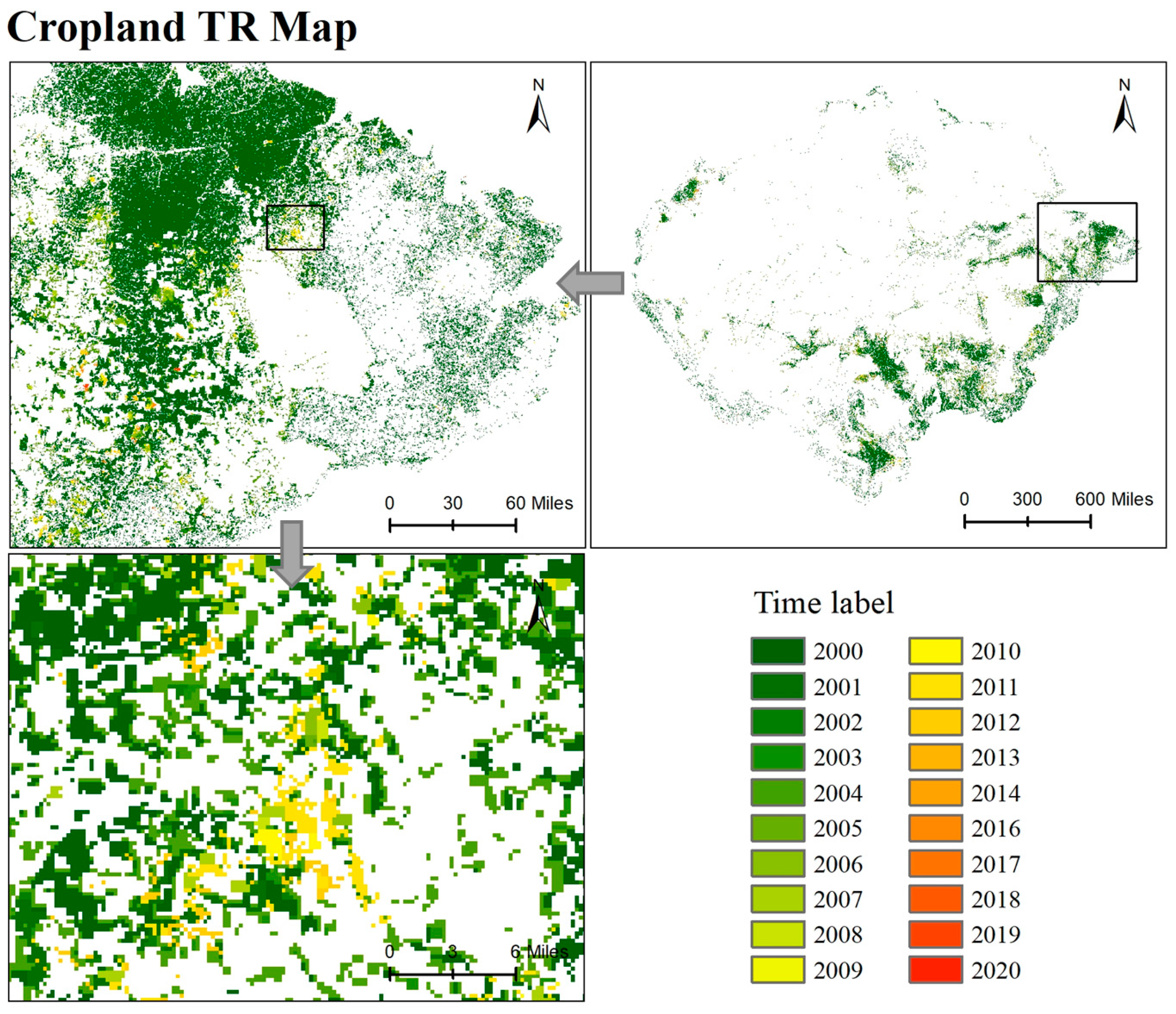
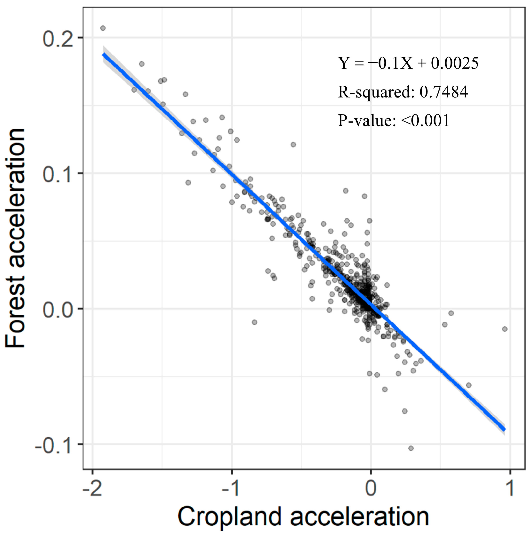
4.2.3. Driving Force of Forest Cover Change

We compared forest and cropland variation characteristics from three perspectives. Firstly, the annual temporal variation in forest and cropland in the Amazon basin showed a symmetric change (Figure 9). The forest area in the Amazon basin demonstrated a downward trend from 2000 to 2008, while the cropland area, on the contrary, displayed an upward trend. The overall forest area in the Amazon basin displayed a slight decrease between 2010 and 2020, while the cropland area displayed a slight increase during the same period. Further, we produced a cropland TR map to compare the spatio-temporal change with that of the forest TR map (Figure 10). The cropland and forest TR maps showed a high similarity of spatial variation characteristics over time. That is, areas of forest loss were usually converted into cropland in the same period. Further, the acceleration of cropland was mapped and linear regression analysis was conducted (Figure 11). The result showed that there was a negative relationship between the acceleration of cropland and forest. The R-squared value reached 0.7484, indicating a strong correlation between them.

5. Discussion

In this study, TR data were proposed to optimize the organizational approach of long-time-series remote sensing data, which was convenient for spatio-temporal analysis and modeling, as well as compensating for the defects of the separate analyses of time and space. Specifically, we used two applications to demonstrate the advantages of TR data. One is NTL in China, representing expansive geographic features. We created the NTL TR map to show the change in urban expansion. Previous studies have shown that Chinese cities and islands have undergone rapid urban expansion [34,35,36], which is consistent with our study mapping NTL TR data. However, we further found that this characteristic was particularly pronounced in coastal cities and some provincial capitals, based on the speed and acceleration maps. In addition, superior to other spatio-temporal analysis methods on urban expansion, such as the expansion contribution rate and expansion intensity index [24,37,38], we found that there was a high speed of expansion on the edge of developed cities in China, while there was a negative acceleration at the center of these cities. This may be due to the limiting of city light by the government and a shift in health awareness in these large urban centers, leading to a reduction in the use of NTL [39,40].
In addition, taking Amazon forest cover as another example, this study identified the spatio-temporal characteristics after mapping the forest TR data, providing explicit information about when and where the forest changed. We observed significant losses in forest cover occurring in the southern and eastern Amazon basin in the period of 2000–2010. The annual rates of deforestation in the Amazon maintained a high level in this decade [41]. Some behaviors, including the development of agriculture and mining, and constructing infrastructure, especially in Brazil, caused large-area deforestation until the related government’s deforestation-control program was enacted [42,43]. The massive forest loss had a great impact on climate change, such as reducing dry season rainfall, which may have directly caused the local temperature to rise [44], even leading to destructive effects on regional forest resilience because of changing climatic conditions [45].
Through the speed and acceleration maps of forest cover and cropland, we found that forest loss was linked to the expansion of cropland in the Amazon basin. Nearly 75% of the forest loss could be attributed to cropland expansion between 2000 and 2020. In addition, according to a survey of soybean expansion in South America, the Brazilian Amazon also experienced the most rapid expansion, where the land that was originally natural vegetation was converted into soybean plantations [46]. Land speculators deforested these areas and usually sold off the timber and converted the land into pasture to further sell it to a soy producer [47]. These deleterious land use changes could contribute to environmental degradation by modifying seasonal water balance and increasing the risk of flooding [48].
Urban expansion and forest loss are both the results of land use change. This transformation is linked to the economic benefits behind it. People, in terms of their own development, tend to seek out land with the greatest economic value. However, this may be wrong when looking at the long term. For example, although the deforestation for cropland in the Amazon basin may promote the economic development of the countries in the region in the short term, the loss may be enormous due to the ecological imbalance caused by forest loss. Therefore, the short-term and long-term benefits should be considered together when planning land use.
As TR data mainly rely on long-time-series data, the temporal integrity and noise of RS data may affect the quality of the production of TR data. Many remote sensing reconstruction methods have been developed [49,50,51], while TR data may help to construct missing and low-quality data from the perspective of spatial–temporal consistency. If geographic features demonstrate evident contraction and expansion, we think that this is predictable for adjacent missing time labels. However, research needs to further explore the prediction technique for TR data.
The TR data have a concise data organization form and, through mapping, these data allow researchers to intuitively understand the spatio-temporal variation characteristics of features. The generation of TR data comprises a simple data-production process, including data preparation, reclassification, feature identification, and data fusion. Similar maps for the urban expansion process have been drawn based on remote sensing technology [35,36,52], but our study systematically puts forward the concept of TR data to visualize the spatiotemporal process. Furthermore, we present the calculation methods of speed and acceleration for TR data analysis. Speed calculation provides a basis for researchers to understand the changing state of features in space and time. Additionally, acceleration helps us to explore the driving mechanism of features. In addition, it is possible to develop other approaches that address TR data to mine more spatial–temporal information.
Time intervals are important in the analysis of time ring data. When we produced TR data using long-time-series RS data, we used the acquisition time of RS data as the time label of TR data, but we also needed to determine the time span of speed and acceleration analysis. Different time spans may affect the mapping result. For that, we, taking NTL TR data in China as an example, reproduced five-year speed and acceleration maps (Supplement Figures S1 and S2). Comparing the 10-year and 5-year maps, we concluded that the longer the time span, the more obvious the characteristics in space and time. However, a shorter time span can provide finer temporal information. Therefore, we advise researchers to balance the temporal resolution and observability of results when choosing the time span to map speed and acceleration.
From our perspective, time ring (TR) data have great application prospects because they can be used to obtain information relating to spatial expansion or contraction over time and can be suitably linked to other data to analyze the change mechanism, which has practical significance in many applications. For instance, lumpy skin disease (LSD), an infectious disease of cattle transmitted by arthropods, has undergone a rapid expansion in its geographic distribution since 2012 [53]. The spatial expansion of LSD has caused substantial economic losses [54] and is closely linked to environmental factors, so we could easily identify the spatio-temporal influencing pattern by mapping the TR data of related factors. Many vector-borne diseases, such as malaria [55,56] and dengue [57,58], as a result of climate change, may spatially expand or contract over time. Additionally, the variational speed regarding space could be different when affected by environmental conditions at different times, meaning that it is usually difficult to determine the influencing relationship [59]. However, the analysis based on TR data may help us to clearly recognize the spatial and temporal characteristics of environmental risk factors associated with vector-borne diseases.
In our study, we emphasized the advantages of using RS data as the data source of TR data, but TR data are also inclusive of other data sources, such as vector features, including point features, line features, or polygon features, in geographic information science (GIS). For instance, we can use yearly OpenStreetMap road data to produce road TR data. Roads can be seen as an expansive feature, usually extending on the basis of the previous roads. This expansion is related to human activity and may cause a series of social environmental problems, so road TR data potentially have great analytic value.
There are some limitations of TR data. Firstly, TR data cannot be applied to all geographic features, as they can only be used for features that undergo spatial expansion or contraction over time. Of course, many geographic features are both expansive and contractive. One TR map struggles to display both of these states simultaneously. However, it is possible to separately exhibit the expansion and contraction of one feature based on TR data. For example, we tend to produce contractive TR maps of forests in the Amazon basin because forest loss is more dominant than forest growth in the region. However, we can also generate a TR map for forest expansion in order to find out if there are areas with a growing forest over time. The difficulty may lie in how to combine forest increases and decreases for interactive analysis, which is expected to be solved in the following study. Secondly, the produced TR data were used to reveal the distribution change in geographic features in space and time, but changes in other feature attributes have been not considered, such as the NDVI value or the strength of nighttime light. Thirdly, TR data are used to display the spatial change in features with time, inevitably leaving out information due to data fusion, but this can be ignored in the analysis of spatio-temporal distribution variation, unless researchers focus on the other attributes of geographic features.

6. Conclusions

This study defined an efficient data structure, namely time ring (TR) data, to reveal the spatio-temporal changes in geographic features based on long-time-series remote sensing data. Common geographic features are either spatially expanding or spatially contracting, so we list two applications to illustrate the practicality of TR data. Firstly, we used NTL remote sensing data as an example to exhibit urban expansion over time by producing a NTL TR map. Cities in eastern China have experienced a rapid expansion since 2000. Beijing, Tianjin, Hebei Province, Shandong Province, and Jiangsu Province exhibited a high acceleration of urbanization. However, in the center of many developed cities, the NTL decreased, revealing laws related to urban development. In addition to revealing the spatio-temporal characteristics of NTL data, a significant aspect is that we can use NTL TR data to perform an exploration of spatio-temporal dynamics, such as the relationships between NTL expansion and population distribution. In addition, taking Amazon forest cover as another example, we illustrated its spatio-temporal variation by mapping forest TR data and demonstrated an applied method of TR data by conducting the calculation of speed and acceleration and using ordinary regression modeling. The results indicate that forest loss in the Amazon basin was more significant between 2000 and 2010 in the southern and eastern regions. Forest loss is closely linked to the expansion of cropland in the Amazon basin, so it is essential to pay more attention to the causes of cropland expansion in order to take measures to avoid continuous forest loss. TR data have the advantages of small data volumes and the easy analysis of spatially and temporally changing characteristics, providing this process with great application prospects. As far as we are concerned, TR data can be applied to environmental health investigation, land use/cover change, disaster monitoring, urban development, and so on, where more analytical methods related to TR data are expected to be discussed.

Supplementary Materials

The following supporting information can be downloaded at: https://www.mdpi.com/article/10.3390/rs15040972/s1.

Author Contributions

Conceptualization, X.L. (Xinhu Li); methodology, X.L. (Xinhu Li); Validation, X.L. (Xinhu Li) and H.B.; formal analysis, X.L. (Xin Liu); data curation, X.L. (Xin Liu); writing—original draft preparation, X.L. (Xin Liu); Writing—review and editing, X.L. (Xin Liu) and X.L. (Xinhu Li); visualization, X.L. (Xin Liu); supervision, X.L. (Xinhu Li) and H.B.; project administration, X.L. (Xinhu Li) and H.B.; funding acquisition, X.L. (Xinhu Li). All authors have read and agreed to the published version of the manuscript.

Funding

This research was funded by the National Natural Science Foundation of China, grant numbers 41671444.

Data Availability Statement

The data presented in this study are available on request from the corresponding author.

Conflicts of Interest

The authors declare no conflict of interest.

References

  1. Wang, J.; Han, P.; Zhang, Y.; Li, J.; Xu, L.; Shen, X.; Yang, Z.; Xu, S.; Li, G.; Chen, F. Analysis on Ecological Status and Spatial–Temporal Variation of Tamarix Chinensis Forest Based on Spectral Characteristics and Remote Sensing Vegetation Indices. Environ. Sci. Pollut. Res. 2022, 29, 37315–37326. [Google Scholar] [CrossRef] [PubMed]
  2. Despini, F.; Ferrari, C.; Bigi, A.; Libbra, A.; Teggi, S.; Muscio, A.; Ghermandi, G. Correlation between Remote Sensing Data and Ground Based Measurements for Solar Reflectance Retrieving. Energy Build. 2016, 114, 227–233. [Google Scholar] [CrossRef]
  3. Militino, A.F.; Ugarte, M.D.; Pérez-Goya, U. An Introduction to the Spatio-Temporal Analysis of Satellite Remote Sensing Data for Geostatisticians. In Handbook of Mathematical Geosciences: Fifty Years of IAMG; Daya Sagar, B.S., Cheng, Q., Agterberg, F., Eds.; Springer International Publishing: Cham, Switzerland, 2018; pp. 239–253. ISBN 9783319789996. [Google Scholar]
  4. Liu, L.; Huang, R.; Cheng, J.; Liu, W.; Chen, Y.; Shao, Q.; Duan, D.; Wei, P.; Chen, Y.; Huang, J. Monitoring Meteorological Drought in Southern China Using Remote Sensing Data. Remote Sens. 2021, 13, 3858. [Google Scholar] [CrossRef]
  5. Gao, Y.; Skutsch, M.; Paneque-Gálvez, J.; Ghilardi, A. Remote Sensing of Forest Degradation: A Review. Environ. Res. Lett. 2020, 15, 103001. [Google Scholar] [CrossRef]
  6. Lin, L.; Di, L.; Zhang, C.; Guo, L.; Di, Y. Remote Sensing of Urban Poverty and Gentrification. Remote Sens. 2021, 13, 4022. [Google Scholar] [CrossRef]
  7. Viana, J.; Santos, J.V.; Neiva, R.M.; Souza, J.; Duarte, L.; Teodoro, A.C.; Freitas, A. Remote Sensing in Human Health: A 10-Year Bibliometric Analysis. Remote Sens. 2017, 9, 1225. [Google Scholar] [CrossRef]
  8. Yang, H.; Kong, J.; Hu, H.; Du, Y.; Gao, M.; Chen, F. A Review of Remote Sensing for Water Quality Retrieval: Progress and Challenges. Remote Sens. 2022, 14, 1770. [Google Scholar] [CrossRef]
  9. He, M.; Xu, Y.; Li, N. Population Spatialization in Beijing City Based on Machine Learning and Multisource Remote Sensing Data. Remote Sens. 2020, 12, 1910. [Google Scholar] [CrossRef]
  10. Xu, D.; Ma, Y.; Yan, J.; Liu, P.; Chen, L. Spatial-Feature Data Cube for Spatiotemporal Remote Sensing Data Processing and Analysis. Computing 2020, 102, 1447–1461. [Google Scholar] [CrossRef]
  11. Xu, C.; Du, X.; Fan, X.; Yan, Z.; Kang, X.; Zhu, J.; Hu, Z. A Modular Remote Sensing Big Data Framework. IEEE Trans. Geosci. Remote Sens. 2022, 60, 1–11. [Google Scholar] [CrossRef]
  12. Koyama, C.N.; Watanabe, M.; Hayashi, M.; Ogawa, T.; Shimada, M. Mapping the Spatial-Temporal Variability of Tropical Forests by ALOS-2 L-Band SAR Big Data Analysis. Remote Sens. Environ. 2019, 233, 111372. [Google Scholar] [CrossRef]
  13. Liu, H.; Hitchcock, D.B.; Samadi, S.Z. Spatio-Temporal Analysis of Flood Data from South Carolina. J. Stat. Distrib. Appl. 2020, 7, 11. [Google Scholar] [CrossRef]
  14. Wang, L.; Jia, Y.; Li, X.; Gong, P. Analysing the Driving Forces and Environmental Effects of Urban Expansion by Mapping the Speed and Acceleration of Built-up Areas in China between 1978 and 2017. Remote Sens. 2020, 12, 3929. [Google Scholar] [CrossRef]
  15. Suleiman, M.S.; Wasonga, O.V.; Mbau, J.S.; Elhadi, Y.A. Spatial and Temporal Analysis of Forest Cover Change in Falgore Game Reserve in Kano, Nigeria. Ecol. Process. 2017, 6, 11. [Google Scholar] [CrossRef]
  16. Ma, Y.; Wang, L.; Liu, P.; Ranjan, R. Towards Building a Data-Intensive Index for Big Data Computing—A Case Study of Remote Sensing Data Processing. Inf. Sci. 2015, 319, 171–188. [Google Scholar] [CrossRef]
  17. Chi, M.; Plaza, A.; Benediktsson, J.A.; Sun, Z.; Shen, J.; Zhu, Y. Big Data for Remote Sensing: Challenges and Opportunities. Proc. IEEE 2016, 104, 2207–2219. [Google Scholar] [CrossRef]
  18. Zhang, Y.; Cheng, J. Spatio-Temporal Analysis of Urban Heat Island Using Multisource Remote Sensing Data: A Case Study in Hangzhou, China. IEEE J. Sel. Top. Appl. Earth Obs. Remote Sens. 2019, 12, 3317–3326. [Google Scholar] [CrossRef]
  19. Ma, J.; Jin, S.; Li, J.; He, Y.; Shang, W. Spatio-Temporal Variations and Driving Forces of Harmful Algal Blooms in Chaohu Lake: A Multi-Source Remote Sensing Approach. Remote Sens. 2021, 13, 427. [Google Scholar] [CrossRef]
  20. Silva, D.; Galvanin, E.A.S.; Menezes, R. Spatio-Temporal Analysis of Land Use/Land Cover Change Dynamics in Paraguai/Jauquara Basin, Brazil. Environ. Monit. Assess. 2022, 194, 400. [Google Scholar] [CrossRef]
  21. Wu, J.; Zhang, Z.; He, Q.; Ma, G. Spatio-Temporal Analysis of Ecological Vulnerability and Driving Factor Analysis in the Dongjiang River Basin, China, in the Recent 20 Years. Remote Sens. 2021, 13, 4636. [Google Scholar] [CrossRef]
  22. Gong, P.; Li, X.; Wang, J.; Bai, Y.; Chen, B.; Hu, T.; Liu, X.; Xu, B.; Yang, J.; Zhang, W.; et al. Annual Maps of Global Artificial Impervious Area (GAIA) between 1985 and 2018. Remote Sens. Environ. 2020, 236, 111510. [Google Scholar] [CrossRef]
  23. Gong, P.; Li, X.; Zhang, W. 40-Year (1978–2017) Human Settlement Changes in China Reflected by Impervious Surfaces from Satellite Remote Sensing. Sci. Bull. 2019, 64, 756–763. [Google Scholar] [CrossRef]
  24. Zhong, Y.; Lin, A.; He, L.; Zhou, Z.; Yuan, M. Spatiotemporal Dynamics and Driving Forces of Urban Land-Use Expansion: A Case Study of the Yangtze River Economic Belt, China. Remote Sens. 2020, 12, 287. [Google Scholar] [CrossRef]
  25. Yin, Z.; Li, X.; Tong, F.; Li, Z.; Jendryke, M. Mapping Urban Expansion Using Night-Time Light Images from Luojia1-01 and International Space Station. Int. J. Remote Sens. 2020, 41, 2603–2623. [Google Scholar] [CrossRef]
  26. Ram, A.K.; Yadav, N.K.; Kandel, P.N.; Mondol, S.; Pandav, B.; Natarajan, L.; Subedi, N.; Naha, D.; Reddy, C.S.; Lamichhane, B.R. Tracking Forest Loss and Fragmentation between 1930 and 2020 in Asian Elephant (Elephas Maximus) Range in Nepal. Sci. Rep. 2021, 11, 19514. [Google Scholar] [CrossRef]
  27. Hugonnet, R.; McNabb, R.; Berthier, E.; Menounos, B.; Nuth, C.; Girod, L.; Farinotti, D.; Huss, M.; Dussaillant, I.; Brun, F.; et al. Accelerated Global Glacier Mass Loss in the Early Twenty-First Century. Nature 2021, 592, 726–731. [Google Scholar] [CrossRef] [PubMed]
  28. Chen, Z.; Yu, B.; Yang, C.; Zhou, Y.; Yao, S.; Qian, X.; Wang, C.; Wu, B.; Wu, J. An Extended Time Series (2000-2018) of Global NPP-VIIRS-like Nighttime Light Data from a Cross-Sensor Calibration. Earth Syst. Sci. Data 2021, 13, 889–906. [Google Scholar] [CrossRef]
  29. Li, C.; Wu, K.; Wu, J. Urban Land Use Change and Its Socio-Economic Driving Forces in China: A Case Study in Beijing, Tianjin and Hebei Region. Environ. Dev. Sustain. 2018, 20, 1405–1419. [Google Scholar] [CrossRef]
  30. Tian, Y.; Yin, K.; Lu, D.; Hua, L.; Zhao, Q.; Wen, M. Examining Land Use and Land Cover Spatiotemporal Change and Driving Forces in Beijing from 1978 to 2010. Remote Sens. 2014, 6, 10593–10611. [Google Scholar] [CrossRef]
  31. Qin, Y.; Xiao, X.; Dong, J.; Zhang, Y.; Wu, X.; Shimabukuro, Y.; Arai, E.; Biradar, C.; Wang, J.; Zou, Z.; et al. Improved Estimates of Forest Cover and Loss in the Brazilian Amazon in 2000–2017. Nat. Sustain. 2019, 2, 764–772. [Google Scholar] [CrossRef] [Green Version]
  32. Defourny, P.; Schouten, L.; Bartalev, S.; Bontemps, S.; Caccetta, P.; De Wit, A.J.W.; Di Bella, C.; Gérard, B.; Giri, C.; Gond, V.; et al. Accuracy Assessment of a 300 m Global Land Cover Map: The GlobCover Experience. In Proceedings of the 33rd International Symposium on Remote Sensing of Environment (ISRSE), Stresa, Italy, 4–8 May 2009; pp. 400–403. [Google Scholar]
  33. Bontemps, S.; Defourny, P.; Radoux, J.; Van Bogaert, E.; Lamarche, C.; Achard, F.; Mayaux, P.; Boettcher, M.; Brockmann, C.; Kirches, G.; et al. Consistent Global Land Cover Maps for Climate Modeling Communities: Current Achievements of the ESA’s Land Cover CCI. In Proceedings of the ESA Living Planet Symposium, Edimburgh, UK, 9–13 September 2013; Volume 2013. [Google Scholar]
  34. Huang, X.; Xia, J.; Xiao, R.; He, T. Urban Expansion Patterns of 291 Chinese Cities, 1990–2015. Int. J. Digit. Earth 2019, 12, 62–77. [Google Scholar] [CrossRef]
  35. Cao, X.; Gao, X.; Shen, Z.; Li, R. Expansion of Urban Impervious Surfaces in Xining City Based on GEE and Landsat Time Series Data. IEEE Access 2020, 8, 147097–147111. [Google Scholar] [CrossRef]
  36. Cao, W.; Zhou, Y.; Li, R.; Li, X.; Zhang, H. Monitoring Long-Term Annual Urban Expansion (1986–2017) in the Largest Archipelago of China. Sci. Total Environ. 2021, 776, 146015. [Google Scholar] [CrossRef]
  37. Hu, Z.-L.; DU, P.-J.; Guo, D.-Z. Analysis of Urban Expansion and Driving Forces in Xuzhou City Based on Remote Sensing. J. China Univ. Min. Technol. 2007, 17, 267–271. [Google Scholar] [CrossRef]
  38. Meng, H.; Zhang, K.; Ba, M.; Wen, D. Spatial Characteristics Analysis of Urban Expansion in Luoyang, China. J. Geogr. Inf. Syst. 2022, 14, 153–174. [Google Scholar] [CrossRef]
  39. Du, X.; Shen, L.; Wong, S.W.; Meng, C.; Yang, Z. Night-Time Light Data Based Decoupling Relationship Analysis between Economic Growth and Carbon Emission in 289 Chinese Cities. Sustain. Cities Soc. 2021, 73, 103119. [Google Scholar] [CrossRef]
  40. Xu, D.; Gao, J. The Night Light Development and Public Health in China. Sustain. Cities Soc. 2017, 35, 57–68. [Google Scholar] [CrossRef]
  41. PRODES 2019 Amazon Deforestation Database. Available online: www.obt.inpe.br/prodes (accessed on 1 September 2022).
  42. Kröger, M. Inter-Sectoral Determinants of Forest Policy: The Power of Deforesting Actors in Post-2012 Brazil. For. Policy Econ. 2017, 77, 24–32. [Google Scholar] [CrossRef]
  43. Fearnside, P.M. The Roles and Movements of Actors in the Deforestation of Brazilian Amazonia. Ecol. Soc. 2008, 13, 23. [Google Scholar] [CrossRef]
  44. Cohn, A.S.; Bhattarai, N.; Campolo, J.; Crompton, O.; Dralle, D.; Duncan, J.; Thompson, S. Forest Loss in Brazil Increases Maximum Temperatures within 50 Km. Environ. Res. Lett. 2019, 14, 84047. [Google Scholar] [CrossRef] [Green Version]
  45. Zemp, D.C.; Schleussner, C.F.; Barbosa, H.M.J.; Rammig, A. Deforestation Effects on Amazon Forest Resilience. Geophys. Res. Lett. 2017, 44, 6182–6190. [Google Scholar] [CrossRef]
  46. Song, X.P.; Hansen, M.C.; Potapov, P.; Adusei, B.; Pickering, J.; Adami, M.; Lima, A.; Zalles, V.; Stehman, S.V.; Di Bella, C.M.; et al. Massive Soybean Expansion in South America since 2000 and Implications for Conservation. Nat. Sustain. 2021, 4, 784–792. [Google Scholar] [CrossRef] [PubMed]
  47. Zalles, V.; Hansen, M.C.; Potapov, P.V.; Stehman, S.V.; Tyukavina, A.; Pickens, A.; Song, X.P.; Adusei, B.; Okpa, C.; Aguilar, R.; et al. Near Doubling of Brazil’s Intensive Row Crop Area since 2000. Proc. Natl. Acad. Sci. USA 2019, 116, 428–435. [Google Scholar] [CrossRef]
  48. Nosetto, M.D.; Paez, R.A.; Ballesteros, S.I.; Jobbágy, E.G. Higher Water-Table Levels and Flooding Risk under Grain vs. Livestock Production Systems in the Subhumid Plains of the Pampas. Agric. Ecosyst. Environ. 2015, 206, 60–70. [Google Scholar] [CrossRef]
  49. Li, S.; Xu, L.; Jing, Y.; Yin, H.; Li, X.; Guan, X. High-Quality Vegetation Index Product Generation: A Review of NDVI Time Series Reconstruction Techniques. Int. J. Appl. Earth Obs. Geoinf. 2021, 105, 102640. [Google Scholar] [CrossRef]
  50. Chu, D.; Shen, H.; Guan, X.; Chen, J.M.; Li, X.; Li, J.; Zhang, L. Long Time-Series NDVI Reconstruction in Cloud-Prone Regions via Spatio-Temporal Tensor Completion. Remote Sens. Environ. 2021, 264, 112632. [Google Scholar] [CrossRef]
  51. Shen, H.; Li, X.; Cheng, Q.; Zeng, C.; Yang, G.; Li, H.; Zhang, L. Missing Information Reconstruction of Remote Sensing Data: A Technical Review. IEEE Geosci. Remote Sens. Mag. 2015, 3, 61–85. [Google Scholar] [CrossRef]
  52. Liu, F.; Zhang, Z.; Zhao, X.; Liu, B.; Wang, X.; Yi, L.; Zuo, L.; Xu, J.; Hu, S.; Sun, F.; et al. Urban Expansion of China from the 1970s to 2020 Based on Remote Sensing Technology. Chinese Geogr. Sci. 2021, 31, 765–781. [Google Scholar] [CrossRef]
  53. Şevik, M.; Doğan, M. Epidemiological and Molecular Studies on Lumpy Skin Disease Outbreaks in Turkey during 2014–2015. Transbound. Emerg. Dis. 2017, 64, 1268–1279. [Google Scholar] [CrossRef] [PubMed]
  54. Machado, G.; Korennoy, F.; Alvarez, J.; Picasso-Risso, C.; Perez, A.; VanderWaal, K. Mapping Changes in the Spatiotemporal Distribution of Lumpy Skin Disease Virus. Transbound. Emerg. Dis. 2019, 66, 2045–2057. [Google Scholar] [CrossRef]
  55. Liu, X.; Song, C.; Ren, Z.; Wang, S. Predicting the Geographical Distribution of Malaria-Associated Anopheles Dirus in the South-East Asia and Western Pacific Regions Under Climate Change Scenarios. Front. Environ. Sci. 2022, 10, 841966. [Google Scholar] [CrossRef]
  56. Gething, P.W.; Smith, D.L.; Patil, A.P.; Tatem, A.J.; Snow, R.W.; Hay, S.I. Climate Change and the Global Malaria Recession. Nature 2010, 465, 342–345. [Google Scholar] [CrossRef] [PubMed]
  57. Ren, Z.; Wang, D.; Ma, A.; Hwang, J.; Bennett, A.; Sturrock, H.J.W.; Fan, J.; Zhang, W.; Yang, D.; Feng, X.; et al. Predicting Malaria Vector Distribution under Climate Change Scenarios in China: Challenges for Malaria Elimination. Sci. Rep. 2016, 6, 20604. [Google Scholar] [CrossRef] [PubMed]
  58. Messina, J.P.; Brady, O.J.; Golding, N.; Kraemer, M.U.G.; Wint, G.R.W.; Ray, S.E.; Pigott, D.M.; Shearer, F.M.; Johnson, K.; Earl, L.; et al. The Current and Future Global Distribution and Population at Risk of Dengue. Nat. Microbiol. 2019, 4, 1508–1515. [Google Scholar] [CrossRef] [PubMed]
  59. Rocklöv, J.; Dubrow, R. Climate Change: An Enduring Challenge for Vector-Borne Disease Prevention and Control. Nat. Immunol. 2020, 21, 479–483. [Google Scholar] [CrossRef]
Figure 1. The general form of time ring (TR) data: (1) for spatially expansive feature; and (2) for spatially contractive feature.
Remotesensing 15 00972 g001
Figure 2. The generation steps of time ring (TR) data.
Remotesensing 15 00972 g002
Figure 3. The data preparation for computing speed and acceleration. The data take the TR data with expansive features as an example. One grid can contain four pixels in this figure.
Remotesensing 15 00972 g003
Figure 4. The urban NTL time ring (TR) map from 2000 to 2020 in China.
Remotesensing 15 00972 g004
Figure 5. The speed and acceleration maps of NTL in China. The negative value in the speed legend represents the speed of NTL reduction, and the negative value of acceleration represents the acceleration of NTL reduction.
Remotesensing 15 00972 g005
Figure 6. The study area of the Amazon basin in South America.
Remotesensing 15 00972 g006
Figure 7. The forest time ring (TR) map from 2000 to 2020 in the Amazon basin.
Remotesensing 15 00972 g007
Figure 8. The speed and acceleration maps of forest loss in the Amazon basin. The negative value in the speed legend represents the speed of forest loss, and the negative value of acceleration represents the acceleration of forest loss.
Remotesensing 15 00972 g008
Figure 9. The temporal variation of forest and cropland in the period of 2000–2020 in the Amazon basin.
Remotesensing 15 00972 g009
Figure 10. The cropland time ring (TR) map from 2000 to 2020 in the Amazon basin.
Remotesensing 15 00972 g010
Figure 11. The linear regression result between the acceleration of cropland and forest.
Remotesensing 15 00972 g011
Disclaimer/Publisher’s Note: The statements, opinions and data contained in all publications are solely those of the individual author(s) and contributor(s) and not of MDPI and/or the editor(s). MDPI and/or the editor(s) disclaim responsibility for any injury to people or property resulting from any ideas, methods, instructions or products referred to in the content.

