
A Multi-Scale Spatial Difference Approach to Estimating Topography Correlated Atmospheric Delay in Radar Interferograms
Abstract
:1. Introduction
2. Model and Estimation Approach
2.1. Model
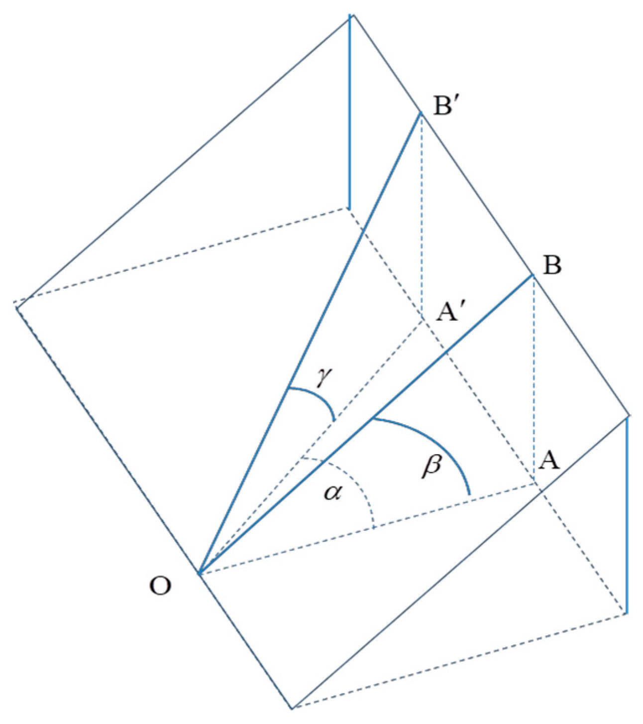
2.2. Estimation Approach
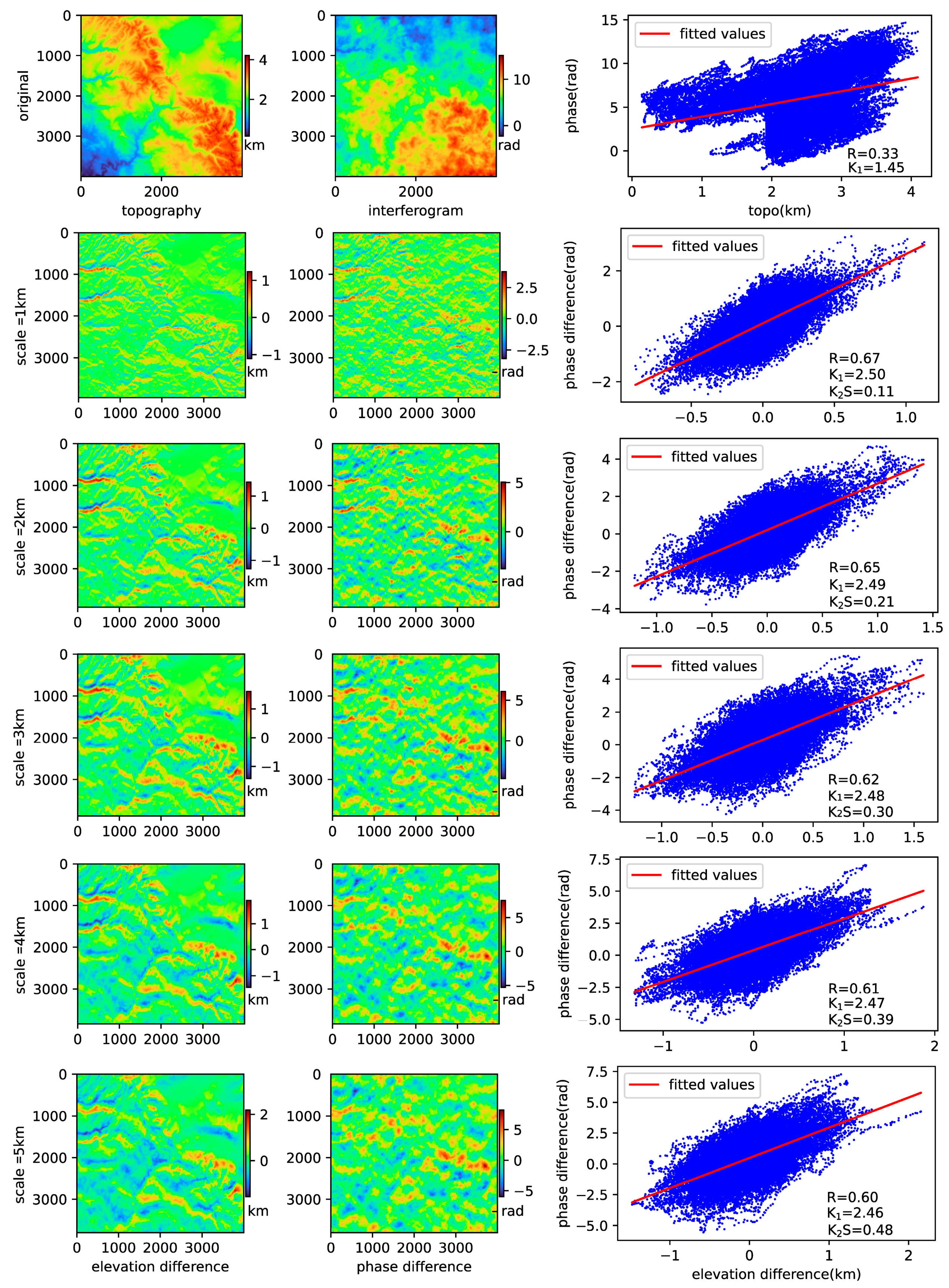
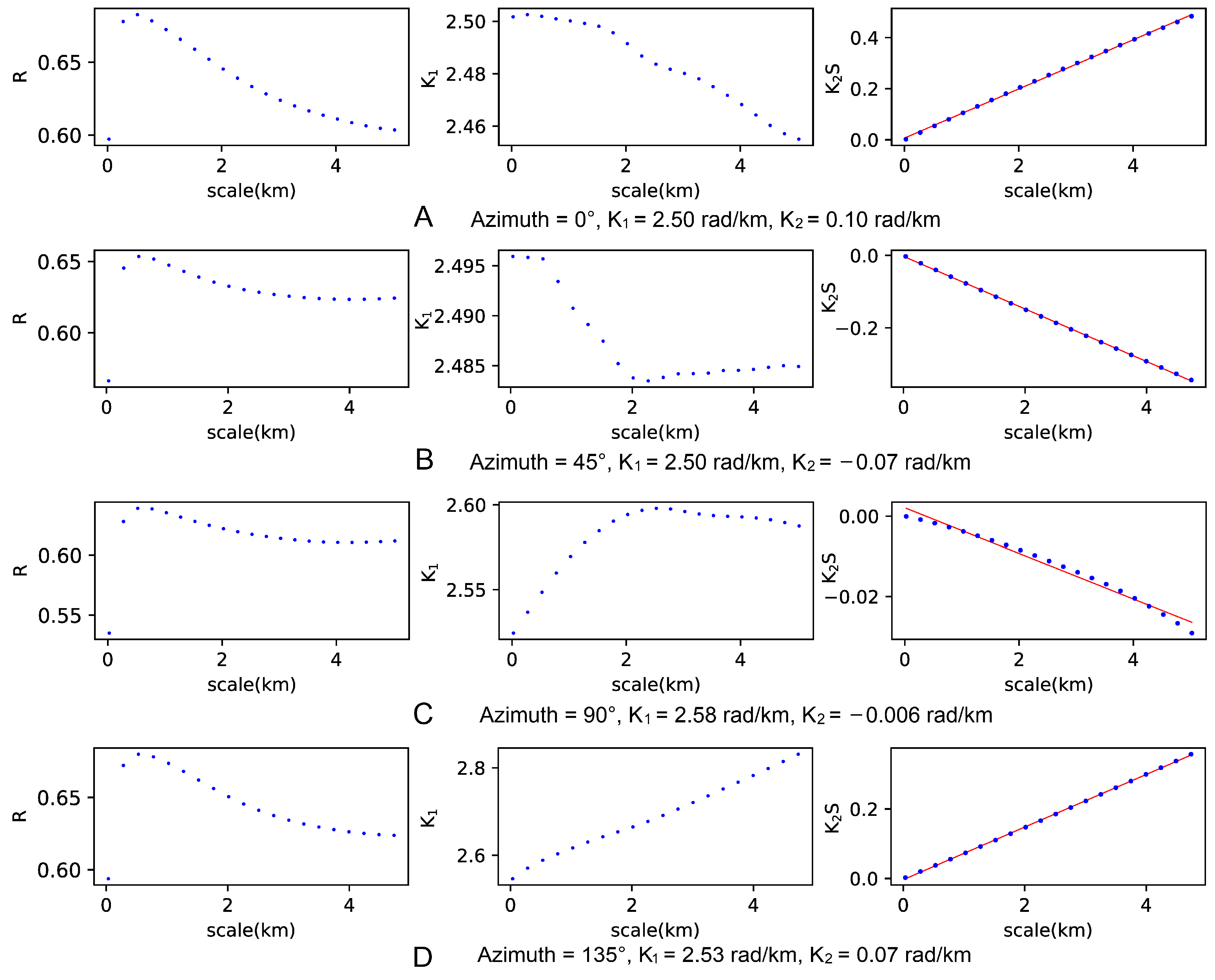
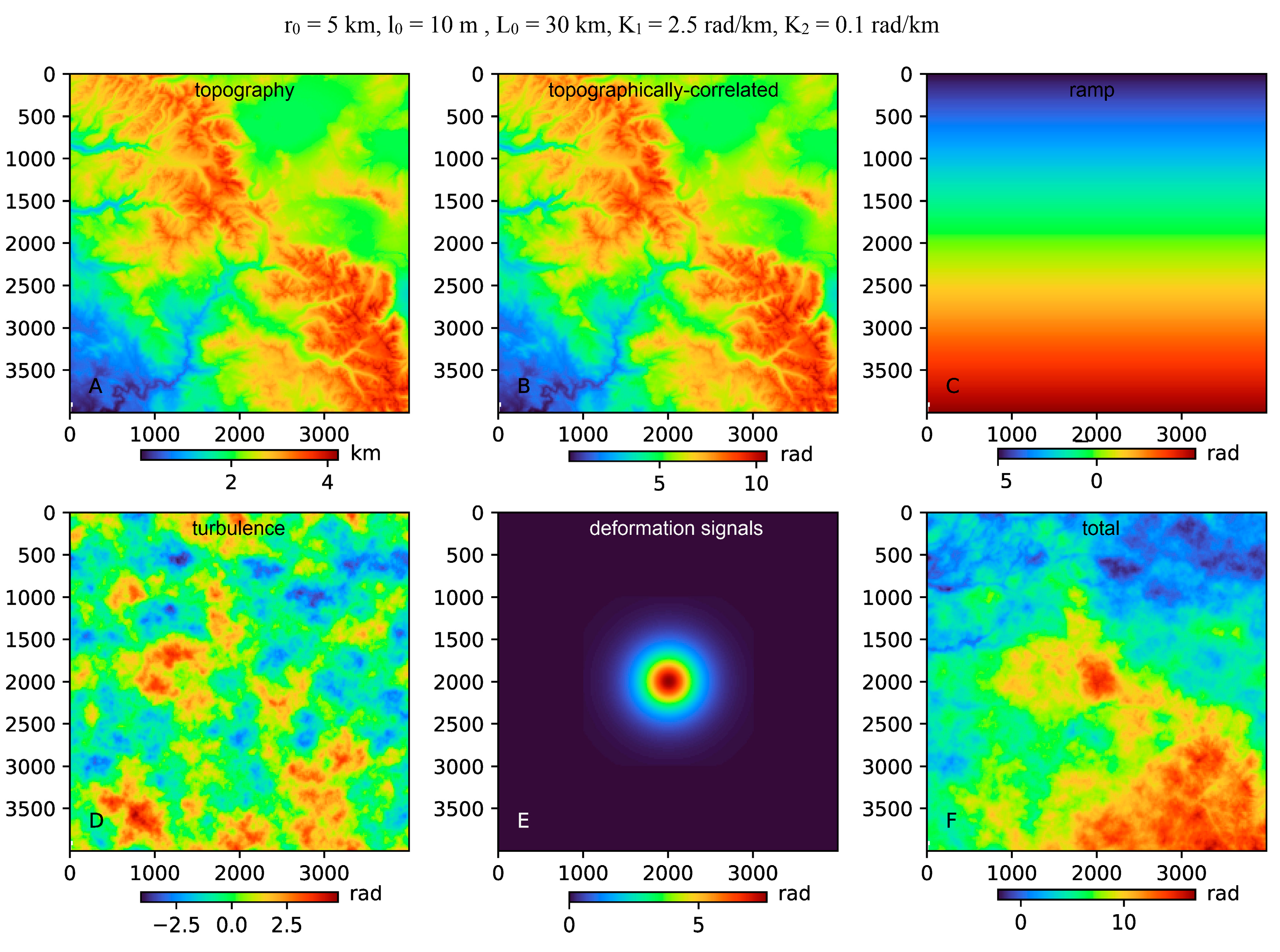
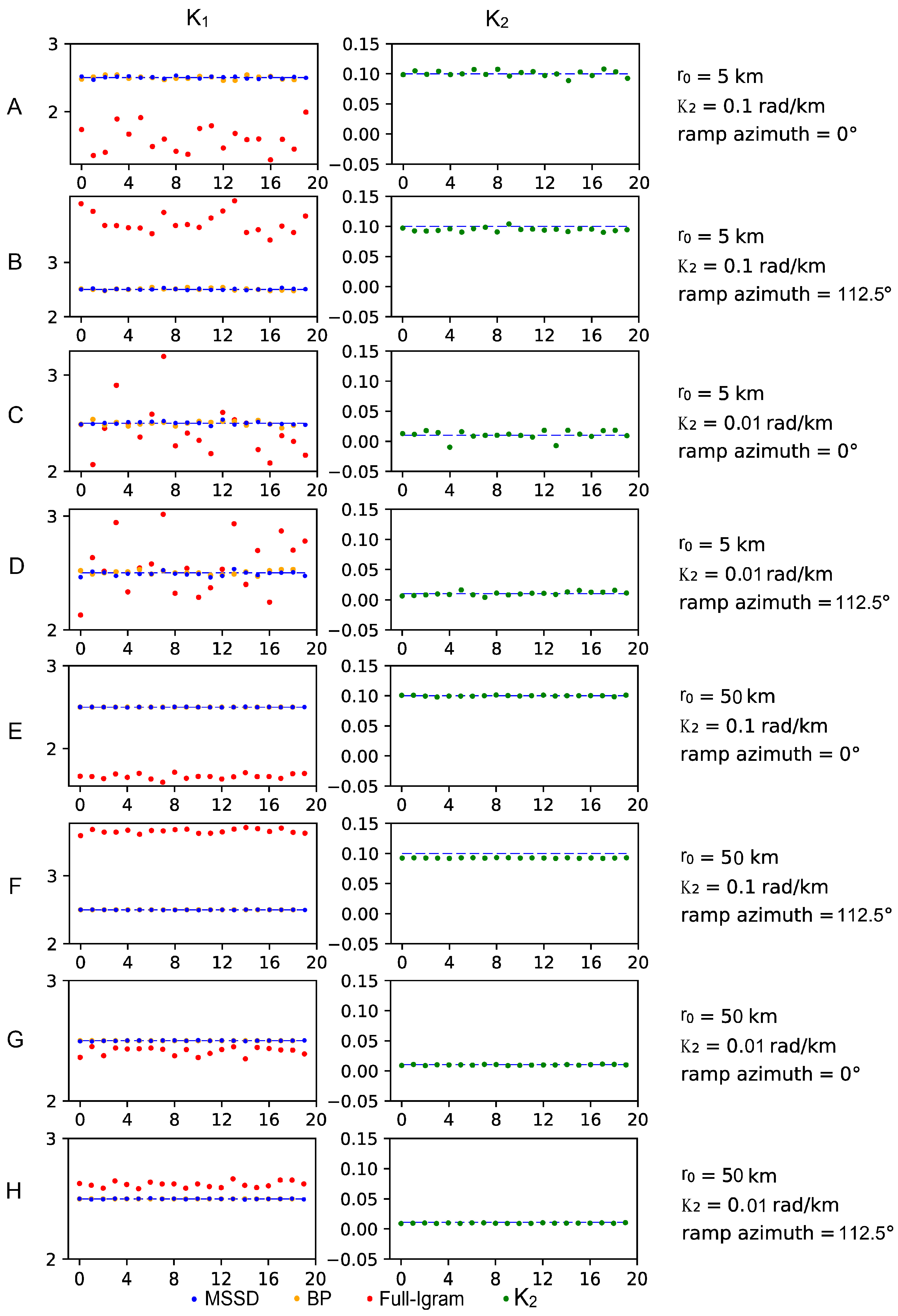
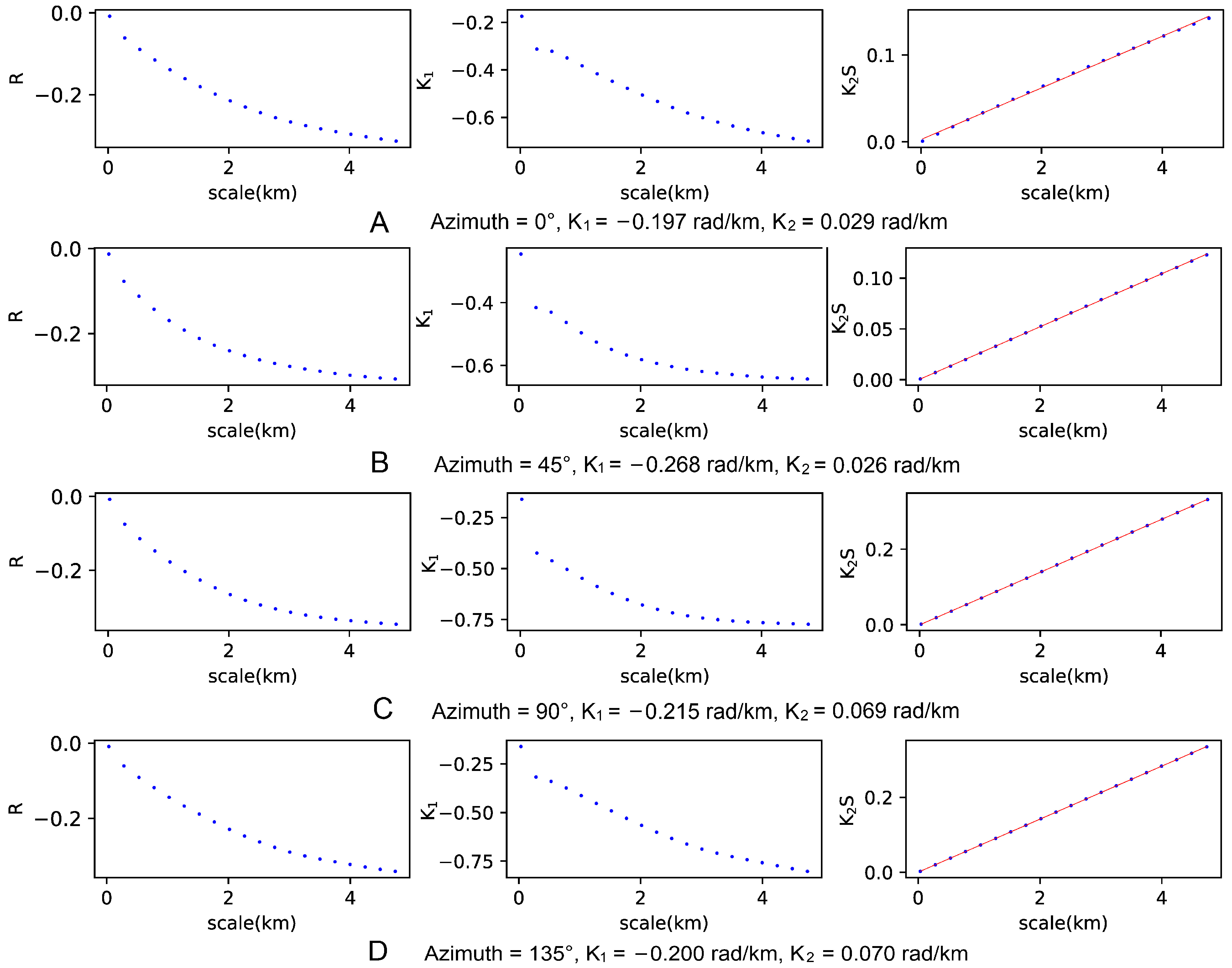
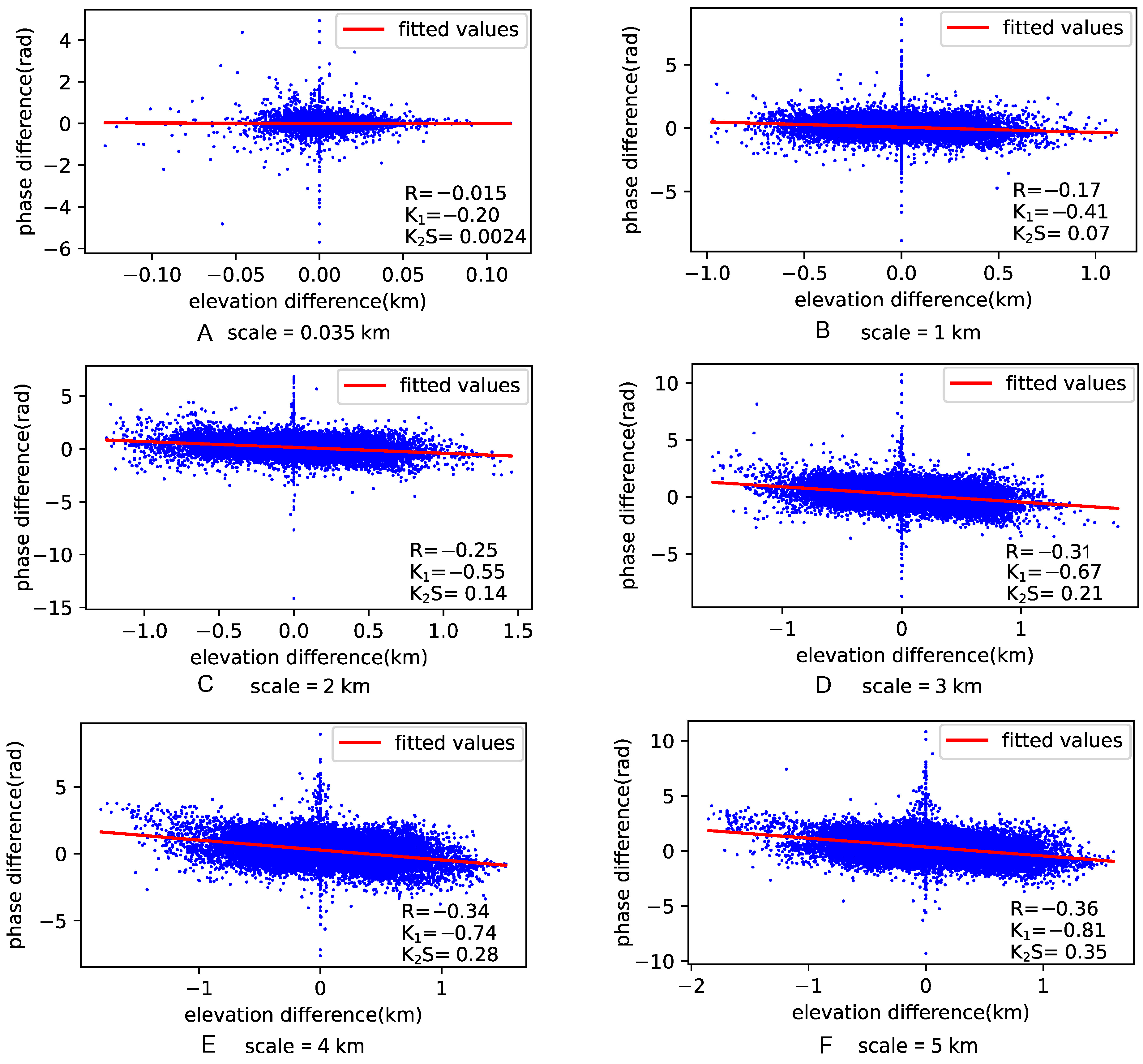
3. Synthetic Test
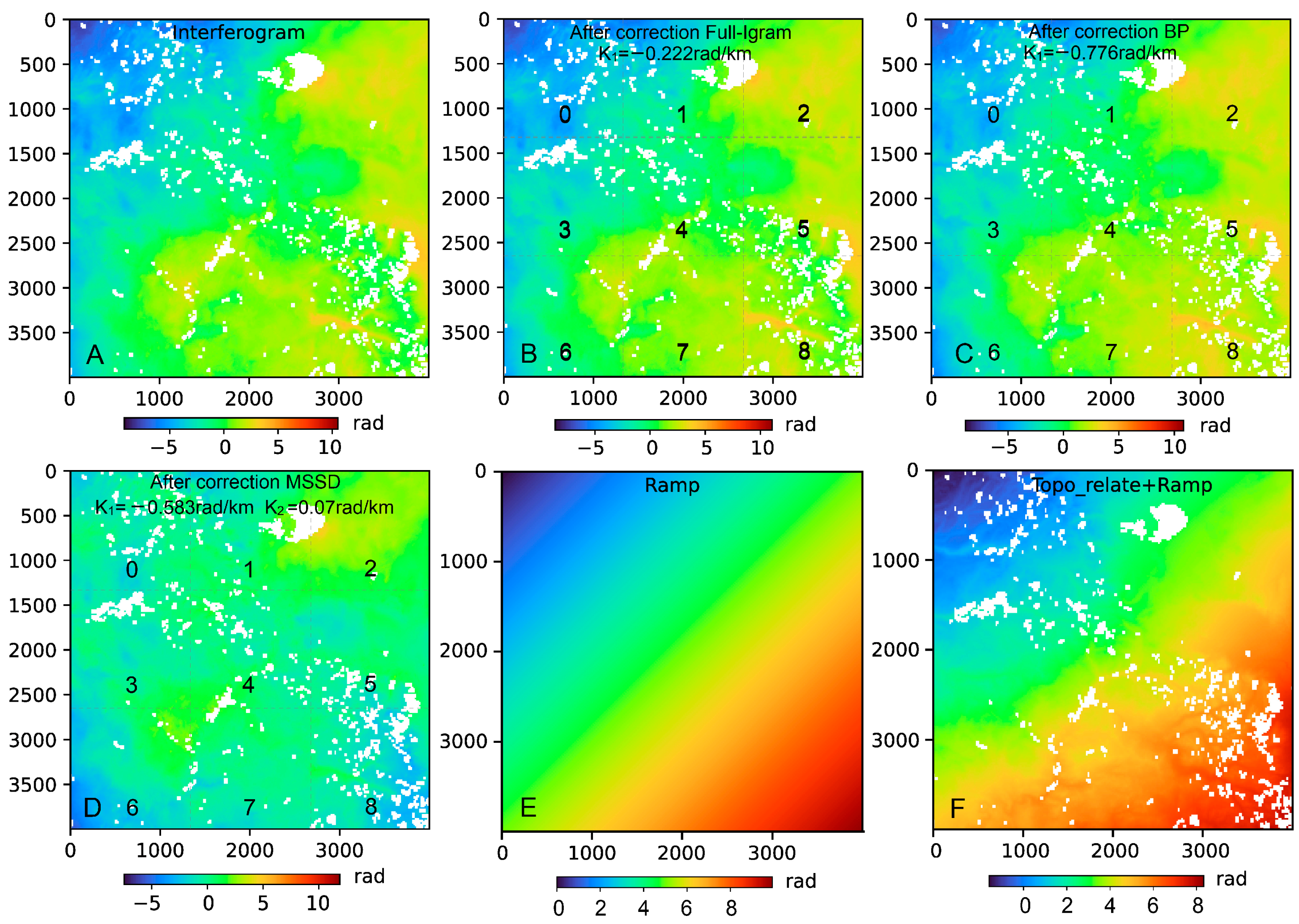
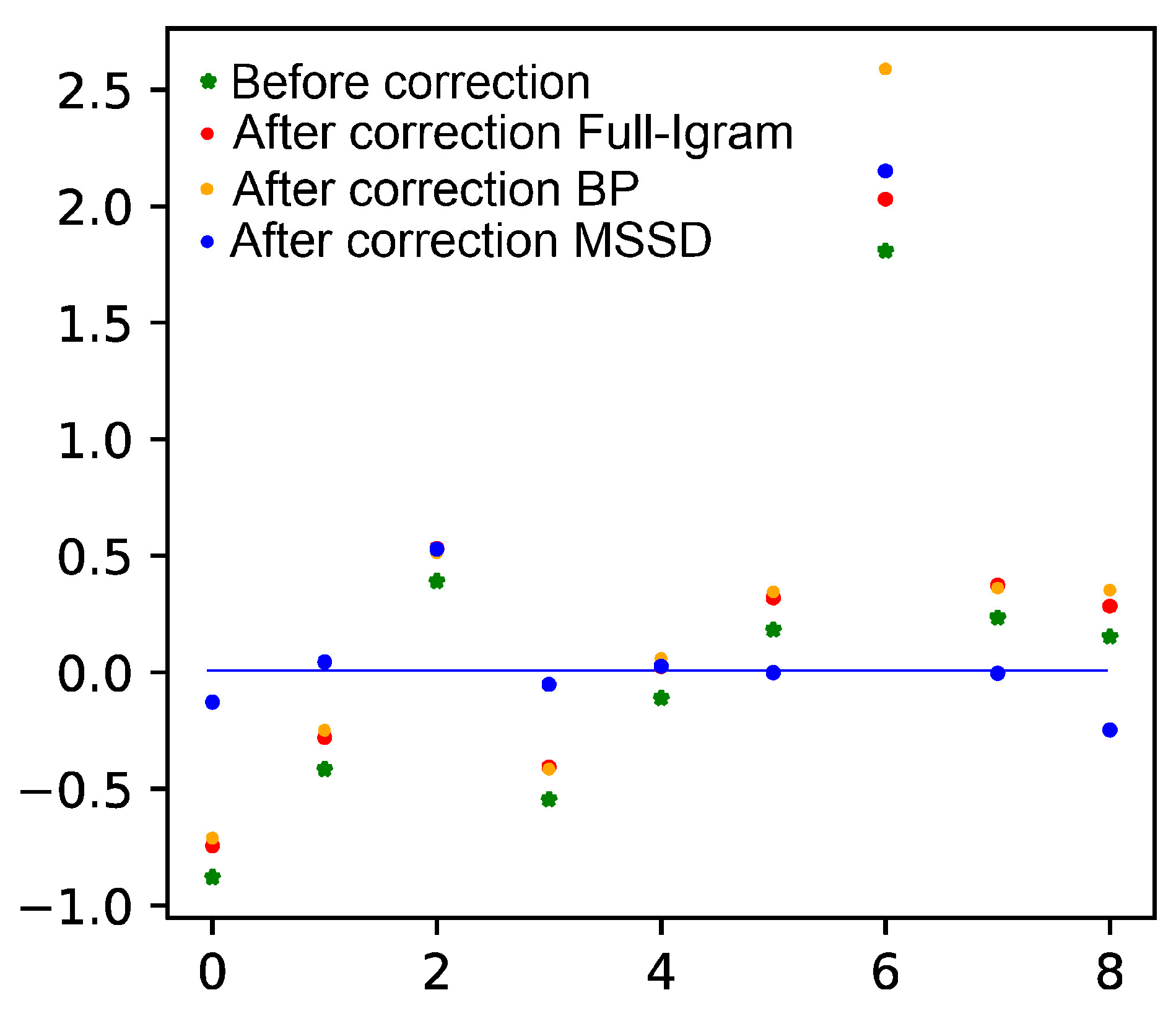
4. Correcting Real Interferogram
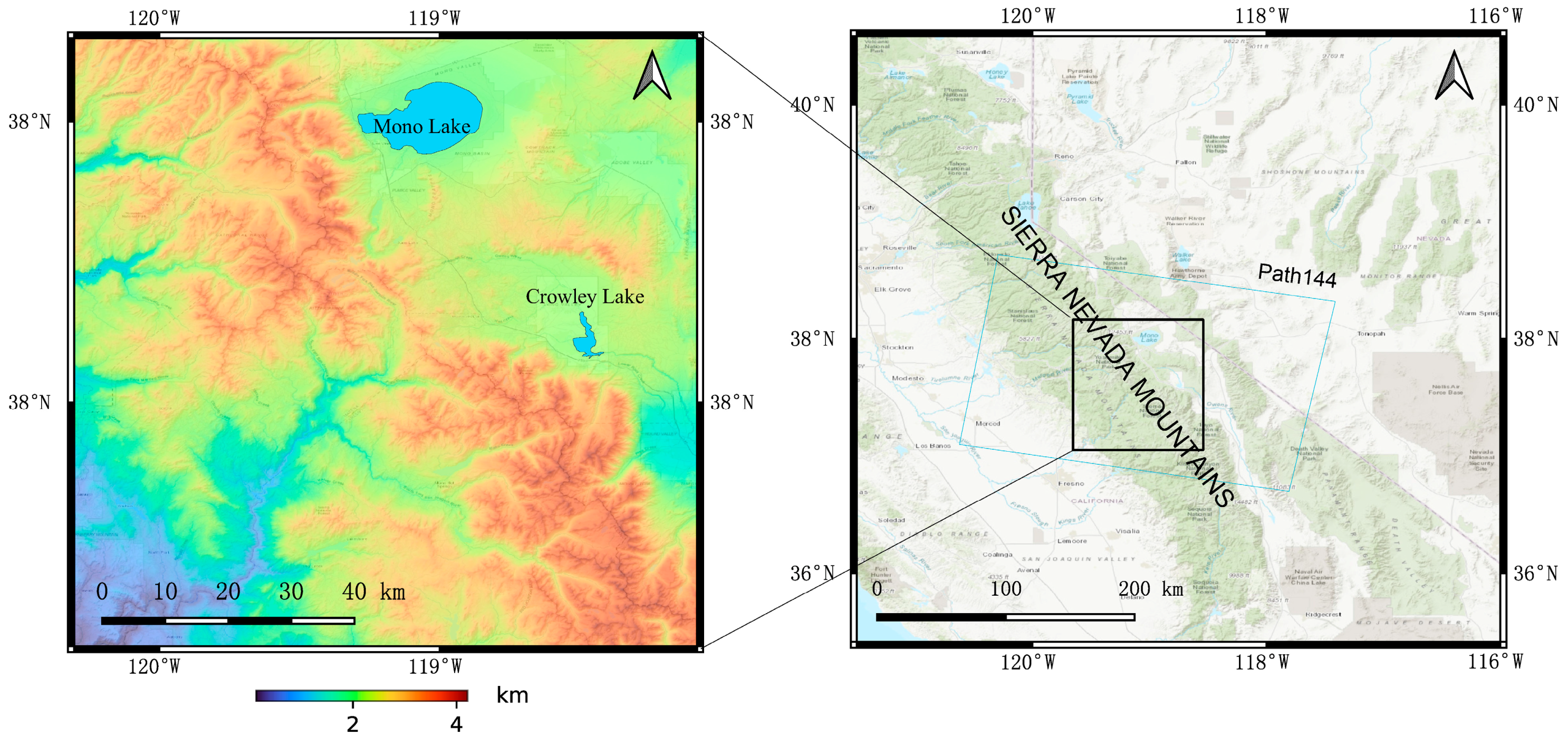
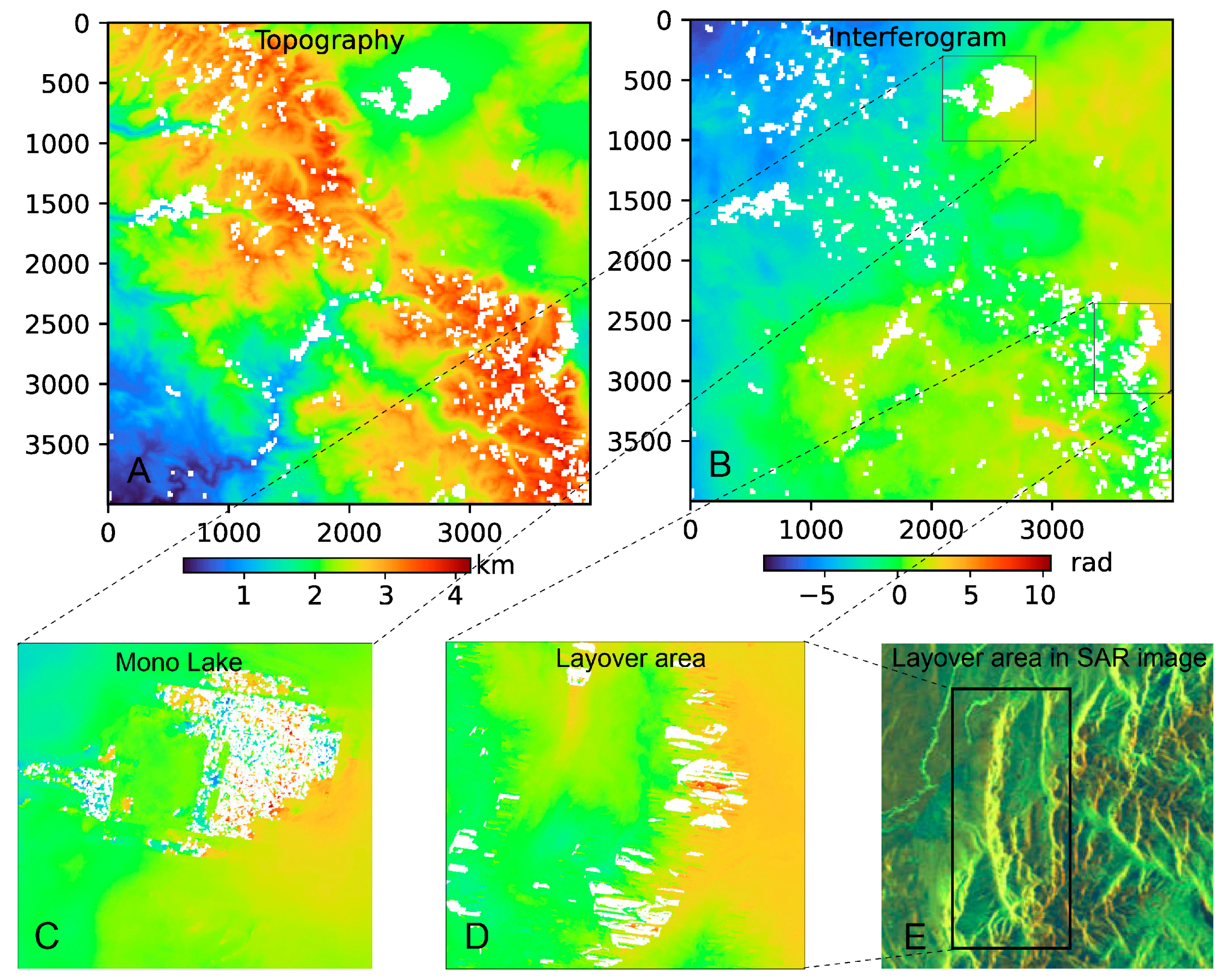
4.1. Sierra Nevada Mountains
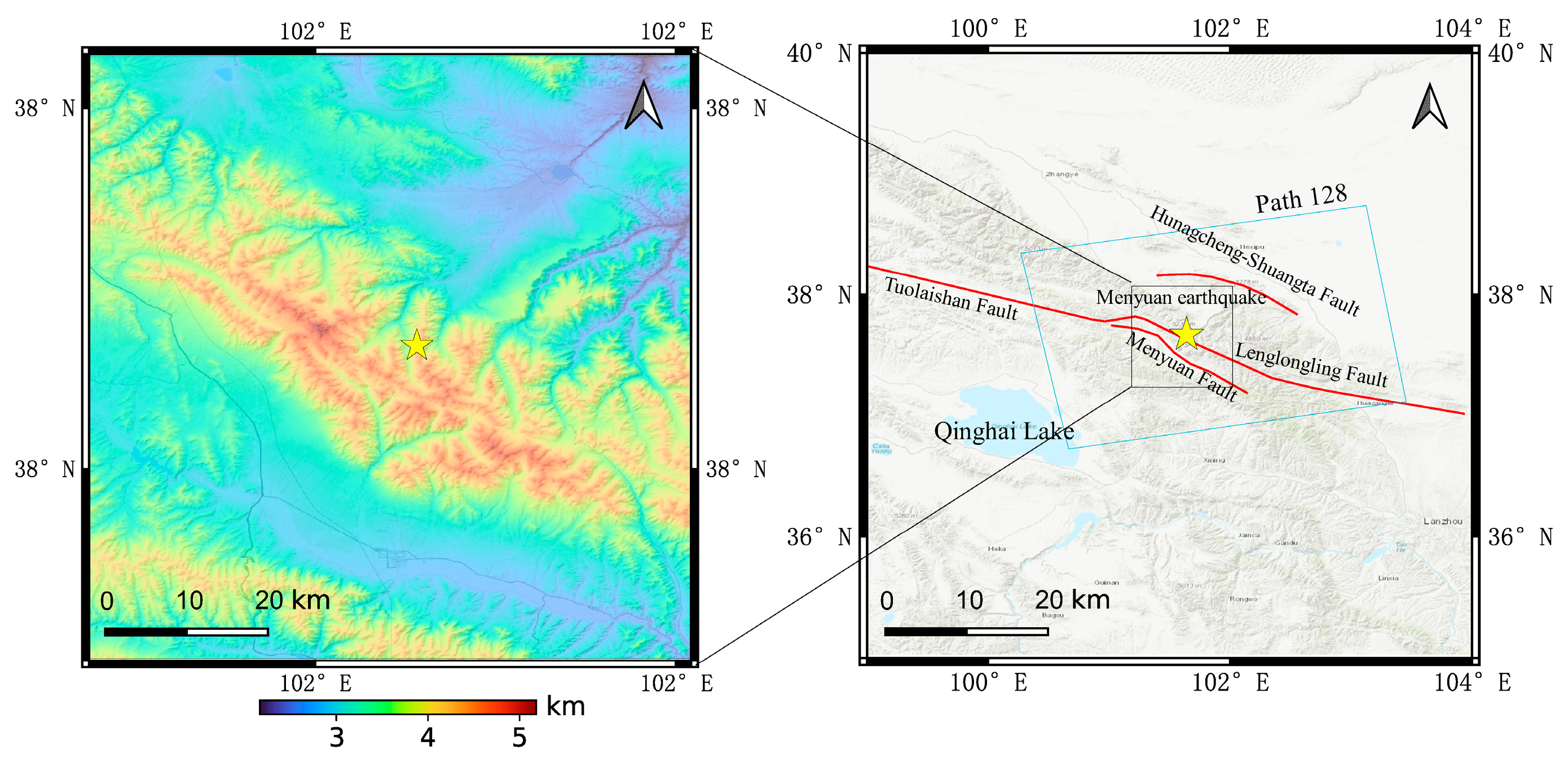
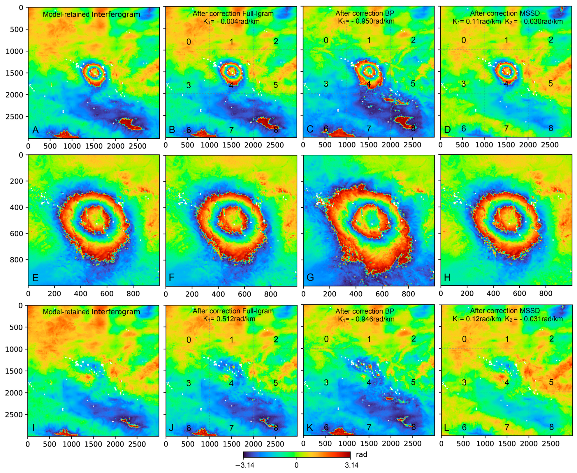
4.2. 2016 Menyuan Earthquake
5. Discussion and Conclusions
Author Contributions
Funding
Data Availability Statement
Acknowledgments
Conflicts of Interest
Appendix A

References
- Gong, W.; Thiele, A.; Hinz, S.; Meyer, F.J.; Hooper, A.; Agram, P.S. Comparison of Small Baseline Interferometric SAR Processors for Estimating Ground Deformation. Remote Sens. 2016, 8, 330. [Google Scholar] [CrossRef]
- Wang, H.; Wright, T.J.; Yu, Y.; Lin, H.; Jiang, L.; Li, C.; Qiu, G. InSAR Reveals Coastal Subsidence in the Pearl River Delta, China. Geophys. J. Int. 2012, 191, 1119–1128. [Google Scholar] [CrossRef]
- Lu, Z.; Fielding, E.; Patrick, M.R.; Trautwein, C.M. Estimating Lava Volume by Precision Combination of Multiple Baseline Spaceborne and Airborne Interferometric Synthetic Aperture Radar: The 1997 Eruption of Okmok Volcano, Alaska. IEEE Trans. Geosci. Remote Sens. 2003, 41, 1428–1436. [Google Scholar] [CrossRef]
- Zhu, L.; Ji, L.; Liu, C.; Xu, J.; Liu, X.; Liu, L.; Zhao, Q. The 8 January 2022, Menyuan Earthquake in Qinghai, China: A Representative Event in the Qilian-Haiyuan Fault Zone Observed Using Sentinel-1 SAR Images. Remote Sens. 2022, 14, 6078. [Google Scholar] [CrossRef]
- Huang, C.; Zhang, G.; Zhao, D.; Shan, X.; Xie, C.; Tu, H.; Qu, C.; Zhu, C.; Han, N.; Chen, J. Rupture Process of the 2022 Mw6.6 Menyuan, China, Earthquake from Joint Inversion of Accelerogram Data and InSAR Measurements. Remote Sens. 2022, 14, 5104. [Google Scholar] [CrossRef]
- Luo, Q.; Perissin, D.; Lin, H.; Li, Q.; Duering, R. Railway Subsidence Monitoring by High Resolution INSAR Time Series Analysis in Tianjin. In Proceedings of the 2011 19th International Conference on Geoinformatics, Shanghai, China, 24–26 June 2011; pp. 1–4. [Google Scholar] [CrossRef]
- Samsonov, S.V.; Tiampo, K.F.; Feng, W. Fast Subsidence in Downtown of Seattle Observed with Satellite Radar. Remote Sens. Appl. Soc. Environ. 2016, 4, 179–187. [Google Scholar] [CrossRef]
- Chen, M.; Tomás, R.; Li, Z.; Motagh, M.; Li, T.; Hu, L.; Gong, H.; Li, X.; Yu, J.; Gong, X. Imaging Land Subsidence Induced by Groundwater Extraction in Beijing (China) Using Satellite Radar Interferometry. Remote Sens. 2016, 8, 468. [Google Scholar] [CrossRef]
- Dong, J.; Zhang, L.; Tang, M.; Liao, M.; Xu, Q.; Gong, J.; Ao, M. Mapping Landslide Surface Displacements with Time Series SAR Interferometry by Combining Persistent and Distributed Scatterers: A Case Study of Jiaju Landslide in Danba, China. Remote Sens. Environ. 2018, 205, 180–198. [Google Scholar] [CrossRef]
- Zebker, H.A.; Rosen, P.A.; Hensley, S. Atmospheric Effects in Interferometric Synthetic Aperture Radar Surface Deformation and Topographic Maps. J. Geophys. Res. Solid Earth 1997, 102, 7547–7563. [Google Scholar] [CrossRef]
- Gray, A.L.; Mattar, K.E.; Sofko, G. Influence of Ionospheric Electron Density Fluctuations on Satellite Radar Interferometry. Geophys. Res. Lett. 2000, 27, 1451–1454. [Google Scholar] [CrossRef]
- Doin, M.-P.; Lasserre, C.; Peltzer, G.; Cavalié, O.; Doubre, C. Corrections of Stratified Tropospheric Delays in SAR Interferometry: Validation with Global Atmospheric Models. J. Appl. Geophys. 2009, 69, 35–50. [Google Scholar] [CrossRef]
- Hanssen, R.F. Radar Interferometry: Data Interpretation and Error Analysis; Springer Science & Business Media: Berlin/Heidelberg, Germany, 2001; Volume 2. [Google Scholar]
- Yu, C.; Li, Z.; Penna, N.T. Interferometric Synthetic Aperture Radar Atmospheric Correction Using a GPS-Based Iterative Tropospheric Decomposition Model. Remote Sens. Environ. 2018, 204, 109–121. [Google Scholar] [CrossRef]
- Li, Z.; Muller, J.-P.; Cross, P.; Fielding, E.J. Interferometric Synthetic Aperture Radar (InSAR) Atmospheric Correction: GPS, Moderate Resolution Imaging Spectroradiometer (MODIS), and InSAR Integration. J. Geophys. Res. Solid Earth 2005, 110. [Google Scholar] [CrossRef]
- Kim, J.-R.; Lin, S.-Y.; Yun, H.-W.; Tsai, Y.-L.; Seo, H.-J.; Hong, S.; Choi, Y. Investigation of Potential Volcanic Risk from Mt. Baekdu by DInSAR Time Series Analysis and Atmospheric Correction. Remote Sens. 2017, 9, 138. [Google Scholar] [CrossRef]
- Tang, W.; Liao, M.; Yuan, P. Atmospheric Correction in Time-Series SAR Interferometry for Land Surface Deformation Mapping—A Case Study of Taiyuan, China. Adv. Space Res. 2016, 58, 310–325. [Google Scholar] [CrossRef]
- Vollrath, A.; Zucca, F.; Bekaert, D.; Bonforte, A.; Guglielmino, F.; Hooper, A.J.; Stramondo, S. Decomposing DInSAR Time-Series into 3-D in Combination with GPS in the Case of Low Strain Rates: An Application to the Hyblean Plateau, Sicily, Italy. Remote Sens. 2017, 9, 33. [Google Scholar] [CrossRef]
- Emardson, T.R.; Simons, M.; Webb, F.H. Neutral Atmospheric Delay in Interferometric Synthetic Aperture Radar Applications: Statistical Description and Mitigation. J. Geophys. Res. Solid Earth 2003, 108, 2231. [Google Scholar] [CrossRef]
- Li, Z.W.; Ding, X.L.; Huang, C.; Zou, Z.R.; Chen, Y.L. Atmospheric Effects on Repeat-Pass InSAR Measurements over Shanghai Region. J. Atmos. Sol.-Terr. Phys. 2007, 69, 1344–1356. [Google Scholar] [CrossRef]
- Lin, Y.N.; Simons, M.; Hetland, E.A.; Muse, P.; DiCaprio, C. A Multiscale Approach to Estimating Topographically Correlated Propagation Delays in Radar Interferograms. Geochem. Geophys. Geosyst. 2010, 11. [Google Scholar] [CrossRef]
- Bekaert, D.P.S.; Walters, R.J.; Wright, T.J.; Hooper, A.J.; Parker, D.J. Statistical Comparison of InSAR Tropospheric Correction Techniques. Remote Sens. Environ. 2015, 170, 40–47. [Google Scholar] [CrossRef]
- DiCaprio, C.J.; Simons, M. Importance of Ocean Tidal Load Corrections for Differential InSAR. Geophys. Res. Lett. 2008, 35. [Google Scholar] [CrossRef]
- Fu, Y.; Freymueller, J.T.; Jensen, T. Seasonal Hydrological Loading in Southern Alaska Observed by GPS and GRACE. Geophys. Res. Lett. 2012, 39. [Google Scholar] [CrossRef]
- Shirzaei, M.; Bürgmann, R. Topography Correlated Atmospheric Delay Correction in Radar Interferometry Using Wavelet Transforms. Geophys. Res. Lett. 2012, 39. [Google Scholar] [CrossRef]
- Delacourt, C.; Briole, P.; Achache, J.A. Tropospheric Corrections of SAR Interferograms with Strong Topography. Application to Etna. Geophys. Res. Lett. 1998, 25, 2849–2852. [Google Scholar] [CrossRef]
- Bürgmann, R.; Rosen, P.A.; Fielding, E.J. Synthetic Aperture Radar Interferometry to Measure Earth’s Surface Topography and Its Deformation. Annu. Rev. Earth Planet. Sci. 2000, 28, 169–209. [Google Scholar] [CrossRef]
- Hanssen, R.F. Atmospheric Heterogeneities in ERS Tandem SAR Interferometry; DEOS Report 98.1; Delft University Press: Delft, The Netherlands, 1998. [Google Scholar]
- Andrews, L.C.; Phillips, R.L. Laser Beam Propagation through Random Media; SPIE: Bellingham, WA, USA, 2005; pp. 58–77. [Google Scholar] [CrossRef]
- Chatterjee, M.R.; Mohamed, F.H.A. Investigation of Profiled Beam Propagation through a Turbulent Layer and Temporal Statistics of Diffracted Output for a Modified von Karman Phase Screen. In Free-Space Laser Communication and Atmospheric Propagation XXVI; SPIE: Bellingham, WA, USA, 2014; Volume 8971, p. 897102. [Google Scholar] [CrossRef]
- Kiyoo, M. Relations between the Eruptions of Various Volcanoes and the Deformations of the Ground Surfaces around Them. Earthq. Res. Inst. 1958, 36, 99–134. [Google Scholar]
- Agram, P.S.; Gurrola, E.M.; Lavalle, M.; Sacco, G.F.; Rosen, P.A. The InSAR Scientific Computing Environment (ISCE): An Earth Science SAR Processing Framework, Toolbox, and Foundry. In Proceedings of the American Geophysical Union, Fall Meeting 2016, San Francisco, CA, USA, 12–16 December 2016. [Google Scholar]
- Chen, C.W.; Zebker, H.A. Phase Unwrapping for Large SAR Interferograms: Statistical Segmentation and Generalized Network Models. IEEE Trans. Geosci. Remote Sens. 2002, 40, 1709–1719. [Google Scholar] [CrossRef]
- Gao, Y.; Tang, X.; Li, T.; Lu, J.; Li, S.; Chen, Q.; Zhang, X. A Phase Slicing 2-D Phase Unwrapping Method Using the L1-Norm. IEEE Geosci. Remote Sens. Lett. 2022, 19, 1–5. [Google Scholar] [CrossRef]
- U.S. Geological Survey (USGS). Available online: http://earthquake.usgs.gov/earthquakes/search/ (accessed on 16 June 2016).
- Global Centroid Moment Tensor Catalogue (GCMT). Available online: http://www.globalcmt.org/CMTsearch.html (accessed on 16 June 2016).
- Li, Y.; Jiang, W.; Zhang, J.; Luo, Y. Space Geodetic Observations and Modeling of 2016 Mw 5.9 Menyuan Earthquake: Implications on Seismogenic Tectonic Motion. Remote Sens. 2016, 8, 519. [Google Scholar] [CrossRef]
- Okada, Y. Surface Deformation Due to Shear and Tensile Faults in a Half-Space. Bull. Seismol. Soc. Am. 1985, 75, 1135–1154. [Google Scholar] [CrossRef]


| Group | A | B | C | D | E | F | G | H | |
|---|---|---|---|---|---|---|---|---|---|
(MSSD) | AVG | 2.503 | 2.505 | 2.500 | 2.492 | 2.500 | 2.499 | 2.500 | 2.500 |
| S.D. | 0.016 | 0.013 | 0.016 | 0.019 | 0.002 | 0.002 | 0.003 | 0.003 | |
BP | AVG | 2.499 | 2.507 | 2.498 | 2.507 | 2.500 | 2.500 | 2.500 | 2.500 |
| S.D. | 0.025 | 0.019 | 0.023 | 0.019 | 0.000 | 0.000 | 0.000 | 0.000 | |
(Full-Igram) | AVG | 1.603 | 3.734 | 2.426 | 2.569 | 1.665 | 3.656 | 2.413 | 2.620 |
| S.D. | 0.200 | 0.192 | 0.268 | 0.252 | 0.031 | 0.032 | 0.033 | 0.024 | |
(MSSD) | AVG | 0.101 | 0.095 | 0.011 | 0.011 | 0.100 | 0.093 | 0.010 | 0.010 |
| S.D. | 0.005 | 0.003 | 0.008 | 0.003 | 0.001 | 0.000 | 0.001 | 0.000 | |
| Sub Region | 0 | 1 | 2 | 3 | 4 | 5 | 6 | 7 | 8 |
|---|---|---|---|---|---|---|---|---|---|
| Original | −0.878 | −0.416 | 0.391 | −0.545 | −0.111 | 0.183 | 1.808 | 0.234 | 0.153 |
| Full-Igram | −0.743 | −0.280 | 0.532 | −0.406 | 0.024 | 0.319 | 2.030 | 0.374 | 0.284 |
| BP | −0.710 | −0.249 | 0.513 | −0.416 | 0.058 | 0.345 | 2.589 | 0.361 | 0.352 |
| MSSD | −0.128 | 0.044 | 0.528 | −0.052 | 0.026 | −0.001 | 2.151 | −0.004 | −0.248 |
| Sub Area | 0 | 1 | 2 | 3 | 4 | 5 | 6 | 7 | 8 |
|---|---|---|---|---|---|---|---|---|---|
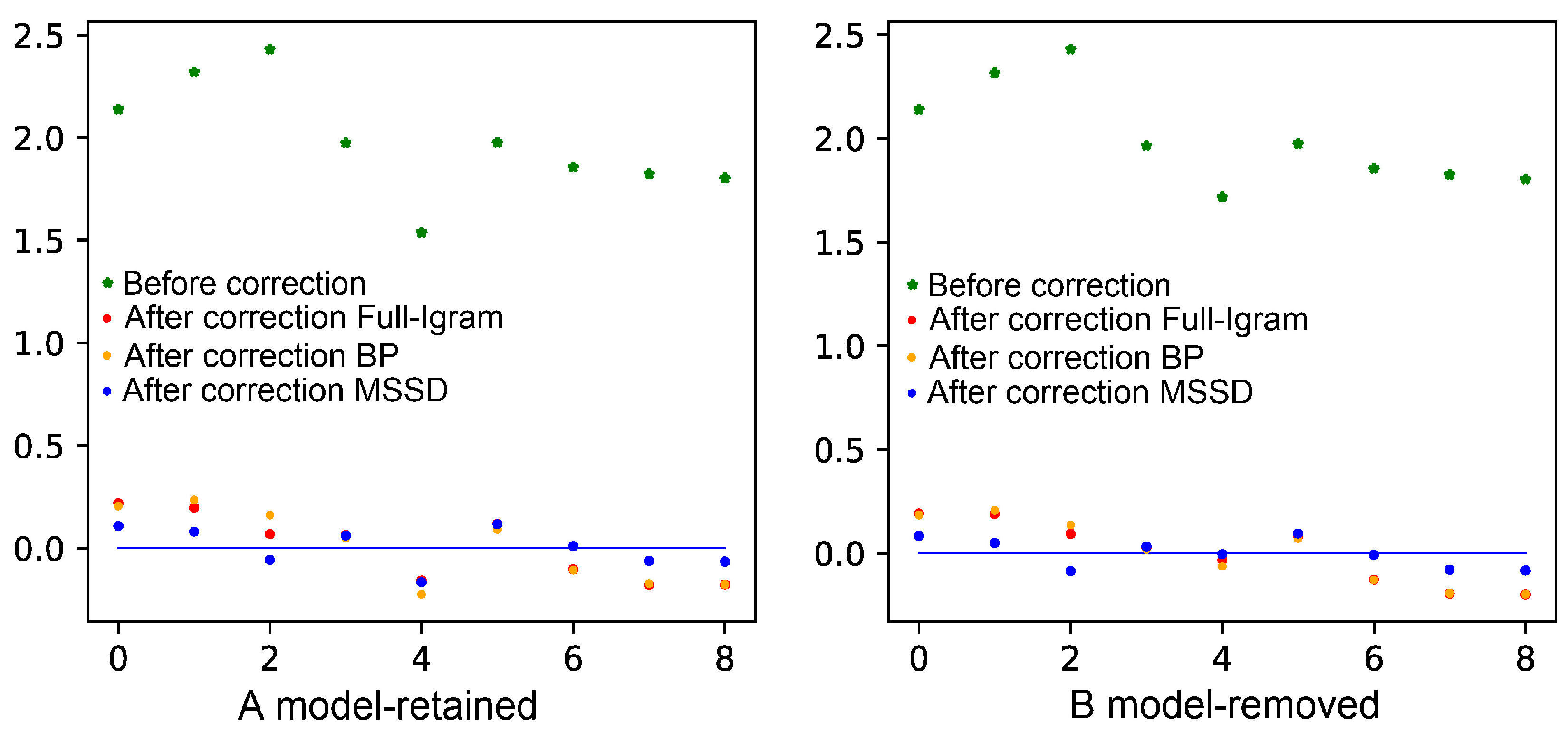
| Orignal | 2.138 | 2.320 | 2.431 | 1.975 | 1.538 | 1.976 | 1.856 | 1.824 | 1.802 |
| Full-Igram | 0.219 | 0.198 | 0.068 | 0.064 | −0.158 | 0.119 | −0.103 | −0.180 | −0.178 |
| BP | 0.205 | 0.235 | 0.161 | 0.049 | −0.226 | 0.090 | −0.107 | −0.173 | −0.177 |
| MSSD | 0.108 | 0.080 | −0.057 | 0.061 | −0.166 | 0.117 | 0.010 | −0.063 | −0.066 |
| Sub Area | 0 | 1 | 2 | 3 | 4 | 5 | 6 | 7 | 8 |
|---|---|---|---|---|---|---|---|---|---|
| Orignal | 2.138 | 2.315 | 2.430 | 1.966 | 1.717 | 1.974 | 1.855 | 1.825 | 1.802 |
| Full-Igram | 0.191 | 0.190 | 0.093 | 0.027 | −0.033 | 0.082 | −0.127 | −0.195 | −0.199 |
| BP | 0.184 | 0.206 | 0.136 | 0.019 | −0.064 | 0.069 | −0.129 | −0.193 | −0.198 |
| MSSD | 0.083 | 0.049 | −0.086 | 0.032 | −0.004 | 0.095 | −0.008 | −0.079 | −0.083 |
Disclaimer/Publisher’s Note: The statements, opinions and data contained in all publications are solely those of the individual author(s) and contributor(s) and not of MDPI and/or the editor(s). MDPI and/or the editor(s) disclaim responsibility for any injury to people or property resulting from any ideas, methods, instructions or products referred to in the content. |
© 2023 by the authors. Licensee MDPI, Basel, Switzerland. This article is an open access article distributed under the terms and conditions of the Creative Commons Attribution (CC BY) license (https://creativecommons.org/licenses/by/4.0/).
Share and Cite
Yu, Z.; Huang, G.; Zhao, Z.; Huang, Y.; Zhang, C.; Zhang, G. A Multi-Scale Spatial Difference Approach to Estimating Topography Correlated Atmospheric Delay in Radar Interferograms. Remote Sens. 2023, 15, 2115. https://doi.org/10.3390/rs15082115
Yu Z, Huang G, Zhao Z, Huang Y, Zhang C, Zhang G. A Multi-Scale Spatial Difference Approach to Estimating Topography Correlated Atmospheric Delay in Radar Interferograms. Remote Sensing. 2023; 15(8):2115. https://doi.org/10.3390/rs15082115
Chicago/Turabian StyleYu, Zhigang, Guoman Huang, Zheng Zhao, Yingchun Huang, Chenxi Zhang, and Guanghui Zhang. 2023. "A Multi-Scale Spatial Difference Approach to Estimating Topography Correlated Atmospheric Delay in Radar Interferograms" Remote Sensing 15, no. 8: 2115. https://doi.org/10.3390/rs15082115