Article

LiteST-Net: A Hybrid Model of Lite Swin Transformer and Convolution for Building Extraction from Remote Sensing Image

1
College of Computer Science, Chengdu University, Chengdu 610106, China
2
Sichuan Urban Informatization Surveying and Mapping Engineering Technology Research Center, Chengdu 610084, China
3
Chengdu Institute of Survey & Investigation, Chengdu 610084, China
*
Author to whom correspondence should be addressed.
Remote Sens. 2023, 15(8), 1996; https://doi.org/10.3390/rs15081996
Submission received: 1 March 2023 / Revised: 6 April 2023 / Accepted: 8 April 2023 / Published: 10 April 2023
(This article belongs to the Special Issue Intelligent Remote Sensing Data Interpretation)

Abstract

:
Extracting building data from remote sensing images is an efficient way to obtain geographic information data, especially following the emergence of deep learning technology, which results in the automatic extraction of building data from remote sensing images becoming increasingly accurate. A CNN (convolution neural network) is a successful structure after a fully connected network. It has the characteristics of saving computation and translation invariance with improved local features, but it has difficulty obtaining global features. Transformers can compensate for the shortcomings of CNNs and more effectively obtain global features. However, the calculation number of transformers is excessive. To solve this problem, a Lite Swin transformer is proposed. The three matrices Q, K, and V of the transformer are simplified to only a V matrix, and the v of the pixel is then replaced by the v with the largest projection value on the pixel feature vector. In order to better integrate global features and local features, we propose the LiteST-Net model, in which the features extracted by the Lite Swin transformer and the CNN are added together and then sampled up step by step to fully utilize the global feature acquisition ability of the transformer and the local feature acquisition ability of the CNN. The comparison experiments on two open datasets are carried out using our proposed LiteST-Net and some classical image segmentation models. The results show that compared with other networks, all metrics of LiteST-Net are the best, and the predicted image is closer to the label.

Graphical Abstract

1. Introduction

Building data are a basic component of geographic information data, which can play an important role in many fields such as urban management, illegal building investigation, demolition cost estimation, etc. Extracting building data from remote sensing images is undoubtedly the fastest and most efficient way to obtain city-level building data. However, even though building data collection from remote sensing images is much more efficient than field measurement, manually obtaining city-level building data remains a huge project. Therefore, decades ago, numerous scholars attempted to use machine learning to automatically extract building data from remote sensing images [1,2,3,4,5,6,7,8]. Although machine learning can automatically extract ground objects from remote sensing images to a certain extent, its performance largely depends on the characteristics of artificial design, for which it is difficult to simultaneously achieve both comprehensiveness and high accuracy. Therefore, the use of machine learning is greatly limited.
In recent years, deep learning has gradually replaced traditional machine learning in the field of computer vision, because of its ability to automatically extract the features required by tasks. The early deep learning network is mainly fully connected; that is, all neurons in each layer are connected with all neurons in the previous layer and the next layer. This kind of network involves a huge amount of computation, which means that the network is not too deep and can only be used for some simple classification tasks. The emergence of LeNet [9] has alleviated this problem by adopting a convolutional structure with shared weights, which substantially reduces the computational complexity. LeNet still has a fully connected layer, which is because it ultimately outputs a probability of 10 numbers. The calculation amount of the fully connected layer is still large, and it does not allow images of unrestricted size to be input. In 2014, researchers from the Visual Geometry Group of Oxford University and Google DeepMind jointly developed a new deep convolution neural network: VGGNet [10]. VGGNet explores the relationship between the depth of a convolution neural network and its performance. The authors constructed a 16–19-layer deep convolution neural network and carried out experiments, demonstrating that increasing the depth of the network can affect the final performance of the network to a certain extent, significantly reducing the error rate. At the same time, the generalization of VGGNet is also very good. VGG remains fully connected. Long et al. [11] proposed a full convolution network in 2015, using convolution to replace the full connection in the network such that images of any size can be input, and the operation speed was improved. FCN realizes semantic segmentation in a real sense, but the segmentation accuracy is not sufficiently high. In the same year, Ronneberger et al. [12] proposed the classic UNet segmentation model based on the FCN network. It is simple, efficient, easy to understand, and easy to build, and can be trained from few data. It has quickly become the mainstream segmentation network in medicine, remote sensing, and other fields. Badrinarayanan et al. [13] proposed a SegNet network model similar to UNet. This model records the index information of the maximum value during max pooling downsampling and then realizes nonlinear upsampling through the corresponding pooling index during decoding, so there is no need to learn at the upsampling stage, and there are fewer network parameters. Zhao et al. [14] proposed a network model called PSPNet, which uses a pyramid pooling module to process feature information of the backbone network and then concatenate them together, and the pyramid pooling module enhances the receptive field of the network and improves the accuracy of segmentation. In 2014, Google released DeepLabV1 [15], in which a dilated convolution is proposed to increase the receptive field. Subsequently, Google has successively released some semantic segmentation network models, such as DeepLabV2 [16] and DeepLabV3 [17], which have increased image segmentation accuracy. Hou et al. [18] proposed a new pooling strategy, called strip pooling, which considers a long but narrow kernel, i.e., 1xN or Nx1. Yu et al. [19] proposed an efficient and effective architecture with a good trade-off between speed and accuracy, termed Bilateral Segmentation Network or BiSeNet V2. The proposal of ViT [20] introduced the transformer [21] from natural language processing to computer vision and broke CNN’s dominant position in this field. The transformer uses only a standard transformer encoder and can achieve the same or even better effect as a CNN, but its structure can only be used for image classification. Zheng [22] proposed a network called SETR, which reshapes the output of the transformer from vectors into an image. Although the performance of SETR is not very good, it is the first attempt to apply a transformer to the field of semantic segmentation. Since every token of the transformer has to be operated with all other tokens, it is very difficult to apply to high-resolution images. In order to solve this problem, Liu et al. [23] proposed a Swin transformer, which limits the operation of the transformer to a small window, instead of the whole image, and improves the operation speed.
With the rapid development of deep learning, many scholars have applied it to the extraction of buildings from remote sensing images, mainly based on convolution neural networks. Most of the innovations optimize the network according to the characteristics of buildings in remote sensing images to improve the accuracy of building extraction. Liu et al. [24] proposed a spatial residual convolution module called spatial residual initiation (SRI). Yi et al. [25] proposed a deep convolutional neural network named DeepResUnet. Diakogiannis et al. [26] proposed a network called Resunet-a. Ye et al. [27] proposed a network named RFA-UNet. Yu et al. [28] proposed an end-to-end network to extract buildings from high-resolution remote sensing images. Liu et al. [29] also used a residual connection network to extract buildings from remote sensing images. Pan et al. [30] proposed a generative countermeasure network based on spatial and channel attention mechanisms. Protopapadakis et al. [31] proposed a deep neural network based on stacked automatic encoder drive and semi-supervised learning. Cheng et al. [32] proposed an automatic building segmentation network named deep active ray network (DARNet). Chen et al. [33] proposed a novel fully convolutional neural network called the Context Feature Enhancement Network (CFENet) to extract buildings from remote sensing images. Na et al. [34] proposed segmentation networks based on a domain adaptive transfer attack (DATA) scheme for building extraction from aerial images. Some scholars also start with the loss function to improve the accuracy of building extraction. Yuan et al. [35] proposed a loss function considering the spatial relationship of pixels. There are also some scholars who start from a lightweight network to improve the running speed of the network. Wang et al. [36] proposed a lightweight U-shaped residual network to extract buildings from remote sensing images on low computing power or a portable device. Chen et al. [37] proposed a dense residual neural network with fewer parameters to extract buildings from remote sensing images. Miao et al. [38] proposed a Feature Residual Analysis Network (FRA-Net) to realize fast and accurate building extraction. Liu et al. [39] proposed a lightweight network for single-image super-resolution. Some scholars have added attention mechanisms to convolutional neural networks to enhance the ability to capture global features [40,41,42,43,44,45], achieving some improvements in performance, but the transformer is a more effective global feature capture structure. With the increasing popularity of transformers, many scholars have also applied them to the interpretation of remote sensing images and achieved good results. Liu et al. [46] proposed a transformer-based model, Informer, to predict rice yield across the Indian Indo-Gangetic Plains. Yuan et al. [47] proposed a multi-scale adaptive network based on the Swin transformer. The network fused the multi-level feature map of the Swin transformer to capture multi-scale information and improved the accuracy of building segmentation. Chen et al. [48] proposed a multi-scale feature learning transformer network. Chen et al. [49] proposed a sparse token transformer to learn the global dependency of tokens in both spatial and channel dimensions. Wang et al. [50] proposed a network called BuildFormer, which fuses the features extracted by the CNN and the features extracted by the transformer to obtain higher segmentation accuracy. However, it is easy to cause gradient explosion in the network, making training difficult.
Although many networks using transformers have been proposed, most are spliced and combined with different models or combined with a CNN, with little improvement to the transformer itself. The combination of different structures can indeed achieve better results, and an important direction of research involves reducing the computation amount of the transformer while preserving its global feature acquisition ability.
The innovations and contributions of this paper are as follows.
(1)
A simplified Swin transformer called Lite Swin transformer is proposed. The Q, K, and V matrices of the transformer are simplified into only a V matrix. The contribution weight between pixels is calculated as VVT. The output feature value is replaced by the V value of the pixel with the largest weight rather than the weighted sum of all pixels. In this way, the model has fewer parameters and faster calculation speed.
(2)
A model integrating Lite Swin transformer and CNN is proposed. In the model, the features extracted from the two are fused at all levels and upsampled step by step.
(3)
We conduct experiments on common open datasets and compare the performance with that of common network models.
The architecture of LiteST-Net, the Lite Swin transformer algorithm, and the dataset used in the experiment are introduced in the next section. The software and hardware equipment used in the experiment, the evaluation metrics of the experiment, and the experimental results of various main network models on the dataset are introduced in the third part. The fourth part is a discussion of the generalization and ablation. The last part is the summary and prospects.

2. Methodology and Materials

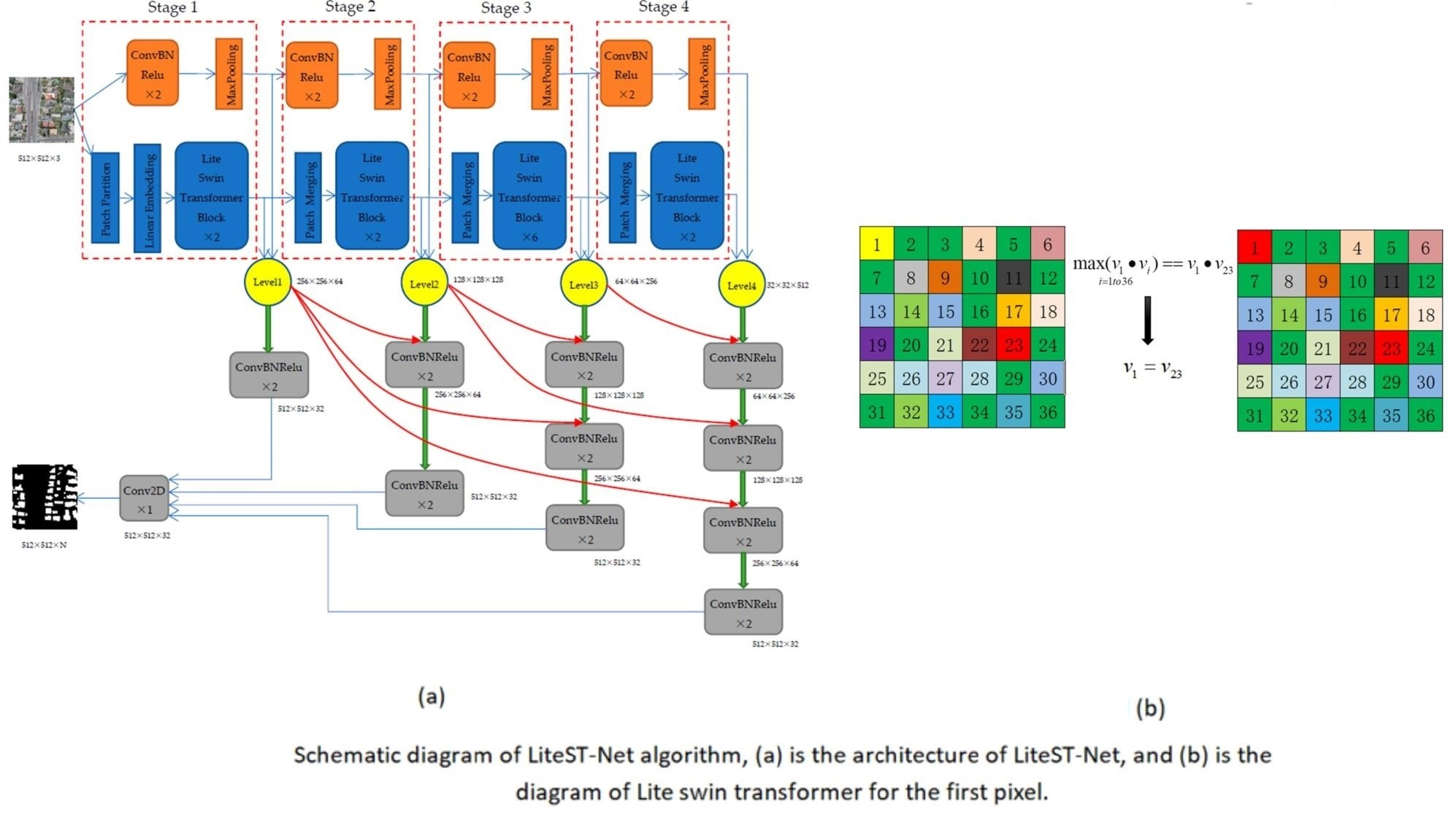
2.1. LiteST-Net Architecture

Although the transformer can better capture global features and become a more popular network structure, the transformer needs to perform a self-attention operation with all points in the process of capturing the global features, which results in an excess of captured information. In order to highlight the global features, the local features are ignored to a certain extent. The convolution operation makes up for this shortcoming. The convolution kernel generally has a size of 3 × 3, with more focus on local features. Therefore, we fuse the convolution and transformer at the same level, upsample step by step, and then fuse different levels to obtain the output.
LiteST-Net consists of three modules in total. The top orange part in Figure 1 is the convolution module that captures local features. There are four stages in total, and four levels of features are output. Each stage consists of two convolution blocks and one MaxPooling block. The kernel size in the convolution block is 3 × 3, BatchNorm is used for batch normalization, and ReLu is used as the activation function. The kernel size of MaxPooling is 2, and the stride is also 2. Therefore, after MaxPooling, the length and width of the feature map will be reduced by half.
The blue part in the middle of Figure 1 is the Lite Swin transformer module, which can also be seen as four stages, where each stage outputs one feature map, and the size of the feature map is consistent with that of the convolution module. The structure of the Lite Swin transformer module is basically the same as that of the Swin transformer, except that the transformer used is the Lite Swin transformer. The algorithm of Lite Swin transformer will be described in detail later. The first stage of Swin transformer module includes a PatchPartition, a LinearEmbedding, and two Lite Swin transformer blocks. The role of PatchPartition is to convert the input image into tokens, while the role of LinearEmbedding is to stretch the dimensions of the tokens to better extract features in Lite Swin transformer. The second and fourth stages of Swin Transformer module contain a PatchMerging block and two Lite Swin transformer blocks. The third stage contains a PatchMerging block and six Lite Swin transformer blocks. PatchMerging results in halving of the length and width of a feature map and doubling the number of channels to save computation and extract more abstract features. The number of Lite Swin transformer blocks in each stage is consistent with the original Swin transformer.
The feature maps of different levels are obtained by fusing features of the convolution module and the Lite Swin transformer module, which is the yellow part in Figure 1. Differently from the way channels are spliced in other papers, in this paper, we directly use the method of adding for fusion to reduce the amount of model parameters.
The gray part in Figure 1 is the decoding module. In all gray rectangular boxes, there are two convolutional blocks, and each convolutional block has convolution with a kernel size of 3 × 3, BatchNorm, and ReLu activation function. The green down arrow represents transpose convolution. The kernel size of transpose convolution is 2, and the stride is also 2. Therefore, after each transpose convolution, the length and width of the feature map will be doubled, and the number of channels will be halved. The red curve represents a skip connection, which means adding two features in the channel. The decoding process is to upsample step by step and fuse the features of the same level at the same time.
The decoding of level 1 involves doubling the length and width and halving the channels through a transpose convolution block (that is, the green arrow down in the figure), and the decoded image is obtained through two convolution blocks. The decoding of level 2 involves doubling the length and width, halving the channels through a transpose convolution block, adding level 1 to it, and then fusing it through two convolution blocks. The above operation is repeated to obtain a decoded image. The process of decoding level 3 is to first double the length and width, halve the channels through a transpose convolution block, add level 2 to it, and then fuse it with two convolution blocks. The above operation is repeated twice, and level 1 added during the process to obtain the decoded image. The process of decoding level 4 is to double the length and width, halve the number of channels through a transpose convolution block, add level 3 to it, and then fuse it with two convolution blocks. The above operation is repeated three times; level 2 and level 1 are added during the process to obtain the decoded image.
The decoding of four levels of features will result in four decoded images, all of which are 512 × 512 × 32 in size. After adding the four decoded images, a convolution layer is used to change the number of channels into the number of segmentation categories (which is two in this paper, namely, buildings and background) so as to obtain the final output.

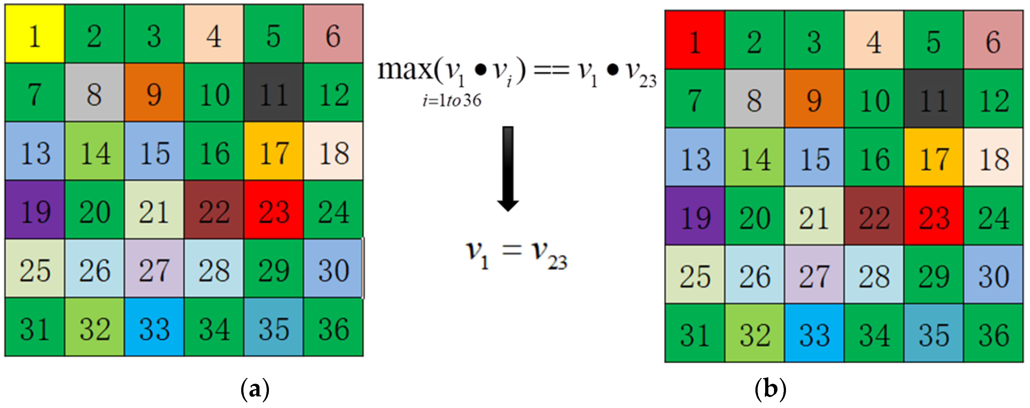
2.2. Lite Swin Transformer

The core of the transformer is the self-attention mechanism, in which the input feature is multiplied by three matrices, WQ, WK, and WV, which are learnable parameters. Therefore, after multiplication, three token matrices, Q, K, and V will be obtained. Q is the query token, K is the queried token, and V is the learned token. We can obtain the weight of the contribution of all other pixels to the pixel by multiplying the q token of a pixel to the k tokens of all other pixels. After normalizing the weight, we multiply it to the corresponding v values of these pixels, respectively, and then add them to get the final contribution value of all pixels to the pixel. The formula is as follows.
Attention ( Q , K , V ) = softmax ( Q K T d k ) V
Since each pixel in the image needs to be multiplied with all other pixels, the results are weighted and summed. With the increase in image size and channels, the amount of computation also sharply increases. If the number of pixels is N, the time complexity is O (N2). Therefore, some algorithms, such as the Swin transformer, limit self-attention to a small window to reduce the amount of computation. However, the consequence of this is that it limits the global feature acquisition ability of self-attention, and even if the operation is limited in a small window, the amount of operation is still relatively large. This means that many computers with a general configuration are unable to use self-attention for model training or the training time is very long.
In order to reduce computing cost, we simplify the three matrices WQ, WK, and WV of self-attention into one WV matrix. The transformer uses QKT to obtain the contribution weight of all pixels to a certain pixel, then multiplies this weight by the corresponding v, and sums to get the feature value of this pixel. Because we remove Q and K, we use VVT to obtain the contribution weight of all pixels to a certain pixel, and because VVT is a symmetric matrix, the theoretical time complexity can be reduced to O (N2/2). As shown in Figure 2, for a two-dimensional token, the contribution weight of token 2 and token 3 to token 1 is the projection of token 2 and token 3 on token 1. This projection can be calculated by the inner product, namely, VVT. However, if V is normalized, the pixel with the largest projection in the V direction of a pixel must be the pixel itself. Therefore, we do not use softmax, which also saves the amount of computation.
After calculating the weight of all pixels to a certain pixel, we do not use the weighted sum of the transformer to calculate the final feature value of the pixel. Inspired by the idea of maximum pooling, we consider that the final contribution value of all pixels to a certain pixel does not need to be weighted and summed by the contribution of all pixels but only replaced by the token v of the pixel with the largest contribution to a certain pixel; that is, it only needs to be replaced by the token v of the pixel that has the largest projection on a certain pixel. As shown in Figure 3, the feature value of pixel 1 is yellow before the Lite Swin transformer, as shown in Figure 3a. If the contribution weight of pixel 23 to pixel 1 is greater than that of all other pixels, then the feature value of the pixel 1 becomes red after the Lite Swin transformer, the same as the feature value of pixel 23, as shown in Figure 3b.
The Lite Swin transformer is represented by pseudocode as Algorithm 1:
Algorithm 1: Lite Swin transformer
Input: feature map, window size
Output: V
1:  Cut the feature map into small feature maps according to the window size
2:  for small feature in small feature maps
3:    Flatten small feature to get a series of Tokens, marked as A
4:    Multiply A by WV to get the V of all Tokens
5:    For each token, calculate the inner product of all other tokens and it, and the formula is VVT
6:    for v in V
7:      take v of the token with the largest inner product to replace its v
8:    end for
9:    reshape V as same as small feature
10:  end for
11:  Splice V as same shape as original input feature map
12:  Move the window position by half the window size, and perform steps 1-11 again
13:  Return V

2.3. WHU Building Dataset and Preprocessing

For our experiment, we selected the aerial dataset of the WHU building dataset [51]. This dataset is labeled by Professor Ji Shunping. The aerial dataset includes more than 220,000 independent buildings extracted from aerial images with a spatial resolution of 0.075 m and covering 450 square kilometers of Christchurch, New Zealand. The original aerial data are from the New Zealand Land Information Service website with a ground resolution of 0.075 m. For training on most computers, the data are sampled to 0.3 m at ground resolution and then cropped into 8189 tiles of 512 × 512 pixels. We divided all tiles into three parts: a training set (4736 tiles, including 130,500 buildings), a validation set (1036 tiles, including 14,500 buildings), and a test set (2416 tiles, including 42,000 buildings). Each tile contains a TIF format image that has three channels and a label that has a single channel.

2.4. Massachusetts Building Dataset and Preprocessing

In order to widely verify the progressiveness of our method, we also chose the Massachusetts Buildings Dataset [52] for experiments. The area covered by this dataset of images corresponding to locations in Boston, USA, corresponds to an area of about 340 square kilometers. There are 151 aerial images in the original dataset, and the size of each image is 1500 × 1500 pixels, with a ground resolution of 1 m and three-channel TIF image format, and the corresponding label is single-channel TIF.
In order to maintain consistency with the image size of the WHU building dataset and not adjust the depth learning model parameters, the original image is cropped to a size of 512 × 512 pixels, one original image is cut into nine images, and the places without pixels are filled with 0 value. A total of 1359 images were obtained after cropping, with 1233 images for the training set and 126 images for the test set.

3. Experiment and Results

3.1. Hardware and Software for Experiment

The computer hardware used in the experiment is configured as follows: the CPU is Intel i5-9400f, the memory is Kingston DDR4 8G, and the GPU is one NVIDIA GeForce RTX 2060 Super 8G. The version of Python is 3.6.8, and both Tensorflow and Pytorch are used as the deep learning framework for model training, depending on the original code of the author.
AdamOptimizer [53] was used for back propagation, and the learning rate was set to 0.0001 during training. The sum of L2 regularization and binary cross entropy was used as the total loss to prevent overfitting. The total loss is shown in Equation (1). The maximum number of training epochs was set to 100. After each epoch, evaluation was performed on the validation dataset. Unlike the stopping standard used in [47], in which training was stopped if the metrics in the validation set no longer increased for 10 consecutive epochs, our stopping standard was that if loss in the validation set was no longer reduced for 10 consecutive epochs, then training was stopped.
TotalLoss = BinaryCrossEntropy + L 2 L 2 = | | w | | 2 2 = i | w i 2 |

3.2. Evaluation Metrics

When the recall value rises, the precision will decline, and vice versa. Therefore, we do not use them alone as the evaluation metric but in combination for F1-score as the evaluation metric. The other two evaluation metrics are the most commonly used, mIoU and Accuracy. The method for calculation of these is shown in Equations (3)–(7).
The formula for mIoU is:
mIoU = 1 N + 1 i = 0 N T P T P + F N + F P
The formula for Accuracy is:
Accuracy = T P + T N T P + T N + F P + F N
The formula for the F1-score is:
F 1 - Score = 2 × P r e c i s o n × R e c a l l P r e c i s o n + R e c a l l
where precision and recall are:
P r e c i s o n = T P T P + F P
R e c a l l = T P T P + F N
In all formulas, N is the number of the foreground. TP is the abbreviation for true positive, which is the number of pixels correctly predicted as the foreground. FP is the abbreviation for false positive, which is the number of background pixels misjudged as the foreground. TN is the abbreviation for true negative, which is the number of pixels correctly predicted as the background. FN is the abbreviation for false negative, which is the number of foreground pixels misjudged as background. In Equation (3), the building and background are regarded as the foreground to obtain IoU, and the average value is then taken as mIoU. The foreground in Equations (5)–(7) is the building.

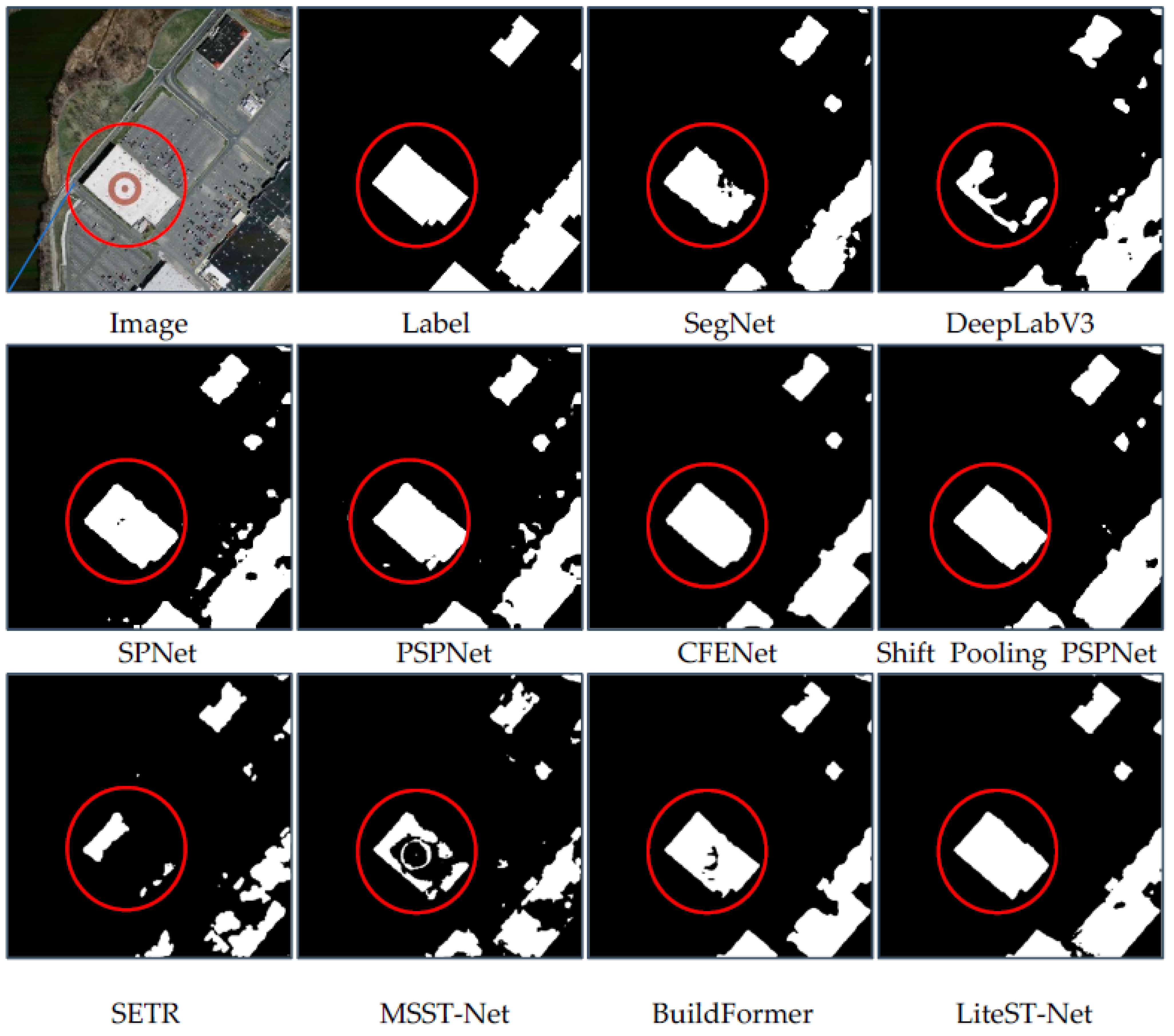
3.3. Results on the WHU Building Dataset

The experimental results on the WHU building dataset are shown in Table 1. It can be seen that our method performs best in three evaluation metrics: mIoU, F1-score, and Accuracy.
The encoders of SegNet, DeepLabV3, SPNet, CFENet, PSPNet, and Shift Pooling PSPNet are pure convolutional neural networks. Among them, the best performer is Shift Pooling PSPNet, followed by CFENet. The worst performer is SegNet, and DeepLab V3 is the second worst. PSPNet and SPNet are in the middle. Shift Pooling PSPNet uses the Shift Pooling pyramid pooling module instead of PSPNet’s pyramid pooling module, so that the pixels at the edge of the pooling grid can also capture complete local features, and the performance is greatly improved. It can be seen from Table 1 that the mIoU of Shift Pooling PSPNet is 2.4% higher than that of PSPNet and 1% higher than that of CFENet, which is the second best performer; the F1-score of Shift Pooling PSPNet is 2.6% higher than that of PSPNet and 1.2% higher than that of CFENet; the Accuracy of Shift Pooling PSPNet is 0.7% higher than that of PSPNet and 0.2% higher than that of CFENet; the mIou, F1-Score, and Accuracy of Shift Pooling PSPNet are 5.3%, 5.9%, and 1.3% higher, respectively, than the worst SegNet. This is enough to show that the receptive field of the network is an important factor to improve the performance of the model. However, the convolution kernel of the convolutional neural network is usually small, and its performance is superior when capturing local features but inadequate for global features.
The introduction of the transformer into the coder of SETR, MSST-Net, BuildFormer, and LiteST-Net can compensate for the deficiency of the convolutional neural network in capturing global features. The SETR and MSST-Net encoders are pure transformers, while BuildFormer and LiteST-Net encoders have both transformers and convolutional neural networks. From Table 1, it can be seen that the performance of encoders with the pure transformer is poor even for MSST-Net, which has relatively good performance among these encoders but is slightly worse than some encoders using only convolutional neural network, while the encoders using both transformer and convolutional neural network have better performance. This shows that although the transformer can capture global information, it needs to calculate with all pixels, so the amount of captured information is huge, and the information of local features will be submerged. If both the transformer and convolutional neural network are used for encoding, they can complement each other so as to achieve better results.
Our proposed LiteST-Net not only uses the transformer and convolution neural network at the same time but also carries out feature fusion at each level, which is more able to capture information of different scales than BuildFormer which only carries out feature fusion at one level. It can be seen from Table 1 that the mIoU of LiteST-Net is 1.9% higher than that of BuildFormer; for F1-score, LiteST-Net is 1.9% higher than BuildFormer; for Accuracy, LiteST-Net is 0.5% higher than BuildFormer, because the value of the evaluation metric has exceeded 90%, so it is excellent to increase 1.9%. On the other hand, compared with Shift Pooling PSPNet, which is the best in the pure convolution neural network, mIoU increased by 3%, F1-score increased by 3.1%, and Accuracy increased by 0.7%, and it can be said that the improvement is significant.
Figure 4 and Figure 5 show the visualization results of some recent deep learning networks on the WHU building test dataset. Figure 4 shows the visualization results for small buildings, and Figure 5 shows the visualization results for large buildings.
From Figure 4, we can see that SegNet, DeepLabV3, PSPNet, SPNet, CFENet, and Shift Pooling PSPNet, which use the convolution as the encoder, rarely miss in the detection of small houses, but we can see that the edges of the houses are too smooth, and the right angles and straight lines of the houses are simplified into curves, as shown in the red rectangular box in Figure 4.
SETR, MSST-Net, and BuildFormer, which use the transformer as the encoder, may miss detection in some cases. As shown in the red rectangle in Figure 4, many pixels of the house are misjudged as background. However, the right angles and straight lines of the house extracted by the network model with transformer as the encoder are more obvious, and the segmentation ability of the house edge pixels is stronger. Because our network model uses the convolution and transformer encoders at the same time and integrates at different levels, it can have the advantages of the convolution and transformer at the same time, so the extracted houses are less likely to be missed in detection, and the edge information of houses can be well retained, matching closest to the labels.
As seen from the house extraction results shown in Figure 5, SegNet has the worst extraction effect and misjudges the different texture parts on both sides of the house as the background. This is basically consistent with the metric ranking in Table 1. Among the other networks using convolution as encoder, DeepLabV3, PSPNet, SPNet, CFENet, and Shift Pooling PSPNet, the best performing is CFENet, which can show the right angle of the building clearly, but there are some errors, as shown in the two spots up the red rectangle in Figure 5. For the other convolution networks, although missed detection is not obvious, the pixel segmentation effect of the edge of the building is poor, and the right angles and straight lines cannot be recognized, as shown in the red rectangle in Figure 5.
The networks with transformer as encoder, SETR, MSST-Net, and BuildFormer, are better than the networks with the convolutional encoder. For the networks with the transformer as the encoder, there are fewer missed houses in detection, and the straight line and right angle of the house edge are clearly identifiable, as shown in the red rectangular box in Figure 5. However, some false detections are also found using this kind of network, as shown in the upper part of the red rectangle in Figure 5, which is particularly obvious for SETR. Our network model uses convolution and transformer encoders at the same time and integrates them at different levels, so it can have the advantages of both convolution and transformer at the same time. Even if there are some false positives, the amount is very small. The straight line and right angle of the edge are basically consistent with the label.

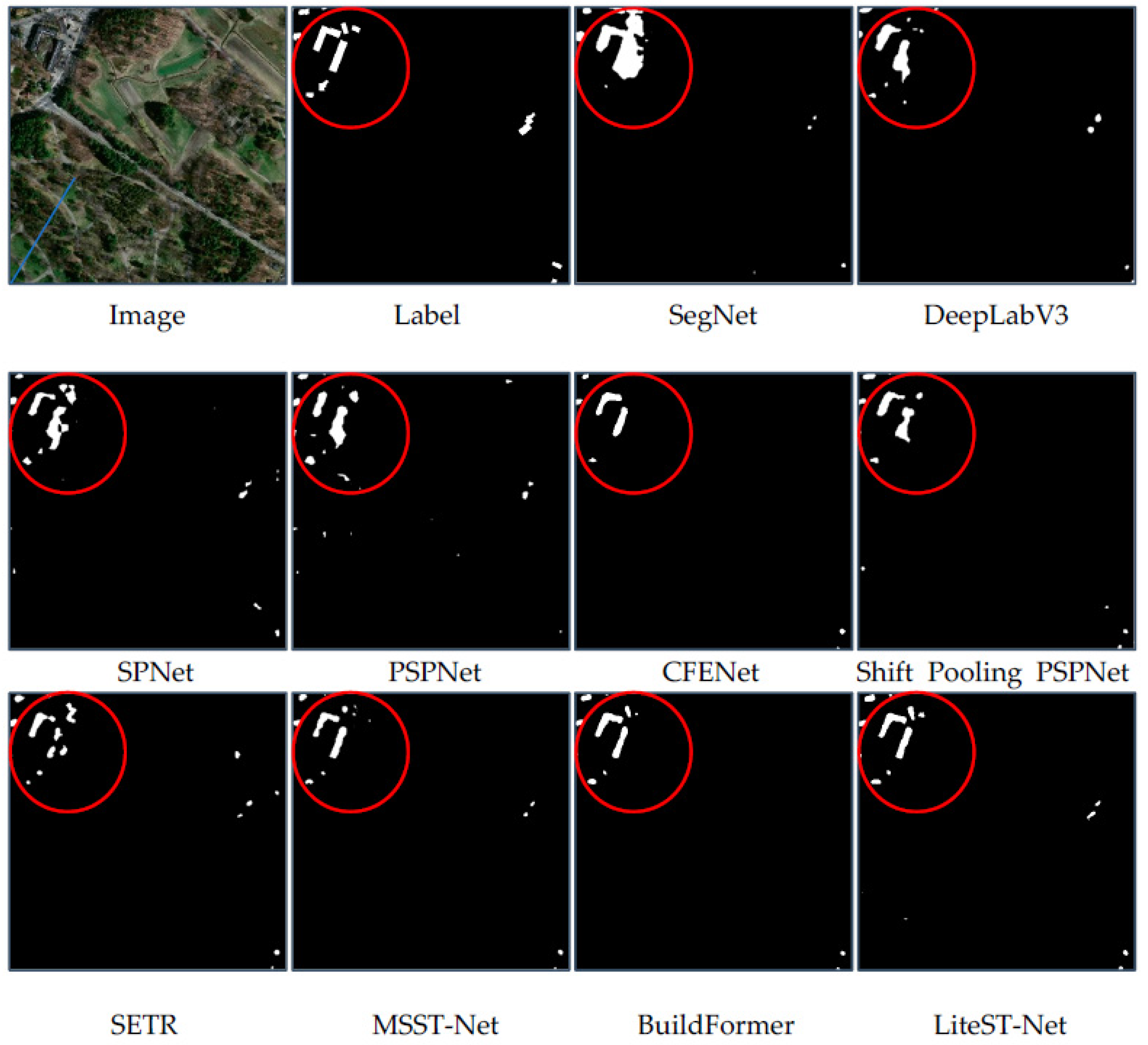
3.4. Results on the Massachusetts Building Dataset

The experimental results on the Massachusetts building dataset are shown in Table 2. It can be seen that our method performs best in the three evaluation metrics of mIoU, F1-score, and Accuracy. Compared with Shift Pooling PSPNet, which is the second best among all encoders, the mIoU increased by 1.1%; the F1-score increased by 1.8%. On the other hand, the mIoU of LiteST-Net is 3.6% higher than that of BuildFormer, which is the second best among transformer encoders; for F1-score, LiteST-Net is 5.4% higher than BuildFormer; for Accuracy, LiteST-Net is 0.5% higher than BuildFormer.
The encoders of SegNet, DeepLabV3, SPNet, CFENet, PSPNet, and Shift Pooling PSPNet are pure convolutional neural networks. Among them, the best performing is Shift Pooling PSPNet; it is consistent with the WHU building dataset, but different from the WHU building dataset; the second best is PSPNet. DeepLab V3 is the worst network, SegNet is the second worst, and CFENet and SPNet are in the middle. The ranking of networks is slightly different from that on the WHU building dataset, but in general, Shift Pooling PSPNet is the best. It can be seen from Table 2 that the mIoU of Shift Pooling PSPNet is 3.6% higher than PSPNet, the second best, and 4% higher than CFENet, the third best; the F1-score of Shift Pooling PSPNet is 4.3% higher than that of PSPNet and 5.6% higher than that of CFENet; the Accuracy of Shift Pooling PSPNet is 1.8% higher than that of PSPNet and 1.2% higher than that of CFENet.
SETR, MSST-Net, BuildFormer, and LiteST-Net introduce transformer into the encoder to compensate for the lack of a convolutional neural network to capture global features. Among them, the encoders of SETR and MSST-Net are pure transformers, while the encoders of BuildFormer and LiteST-Net have both transformers and convolutional neural networks. From Table 2, it can be seen that the performance of the pure transformer encoder is poor. Even the good MSST-Net among them is slightly worse than many encoders that only use the convolutional neural network. This is different from the performance of the WHU building dataset. We find that the performance of the pure transformer network is not as good as that of the pure convolution neural network on the dataset with low labeling accuracy, and the error tolerance is lower than that of CNN. The encoder using both transformer and convolutional neural network has better performance, which shows that this network has better error-tolerance ability even on the dataset with low labeling accuracy.
Figure 6 shows the visualization of networks for large buildings on the Massachusetts building dataset. DeepLabV3 and SETR have the worst performance on the large buildings, with a high rate of false negative. MSST-Net also has a high rate of false negative on large buildings. This shows that the false negative of these three networks will increase on the dataset with low labeling accuracy and low resolution. For the rest of the network models, except for a small amount of false negative in SegNet and BuildFormer, most of the network models can detect complete large houses, as shown in the red circle in Figure 6.
From all the visual images on the test data of Massachusetts buildings, we can see that the performance of our LiteST-Net is the best; there are basically no false negatives, the house edges are very clear, and the straight lines and right angles of the house are clear. This is consistent with the results on the WHU building dataset.
Figure 7 shows the visualization of small buildings on the Massachusetts building dataset. Due to the fact that networks using convolutional encoders pay more attention to local features, there are many false positive pixels in the prediction of small buildings, especially in SegNet. The least false positive pixels are in CFENet, but they have some false negative pixels, as shown in the prediction results in the red circle in Figure 7. Networks using transformer as an encoder have a stronger ability to capture global features, so there are far fewer false positive pixels. Of these, SETR is the worst but it is also better than most convolutional networks. BuildFormer and LiteST-Net have the fewest false positive pixels, but BuildFormer has some false negative pixels.
From all the images, we can see that the LiteST-Net proposed by us is also the best in extracting small buildings, with not only the fewest false positive pixels but also the fewest false negative pixels, and it is closest to the label.

4. Discussion

4.1. Ablation Experiment

In order to directly compare the complexity of the models, we use get_ model_ complexity_ info function in ptflops library to obtain the parameter amounts of several models that perform well on the WHU building dataset, as shown in Table 3.
From the table, we can see that MSST-Net has the least number of parameters, only 16.28 M. CFENet has highest parameter amount, at 44.06 M. If our network LiteST-Net uses the original transformer algorithm, the parameter amount is 20.97 M, and when Lite Swin transformer is used, since the three matrices Q, K, and V are simplified into a V matrix, the parameter amount is reduced to 18.03 M. Although the parameter amount of our LiteST-Net is not the least, it is the second least and only 1 M more than the least, MSST-Net. Therefore, it is very worthwhile to increase the segmentation accuracy by adding only 1.75 M parameters.
In order to verify whether the performance would decrease after reducing the parameter, we conducted an ablation experiment on the WHU building dataset. In the experiment, we used the same LiteST-Net network, including the same decoding structure, the same training strategy, same loss function, etc.
The experimental results in Table 4 show that when we use the original Swin transformer fused by multi-level convolutional, the mIoU is 91.8, F1-score is 92.2, and Accuracy is 98.3. When using our proposed Lite Swin transformer fused by multi-level fusion, all metrics have been improved by 0.1 to 0.3. Although the improvement is not significant, at least it has been proven that our method does not lose accuracy while reducing weight. When using Lite Swin transformer to fuse with the final level of convolution, the mIoU is 91.3, F1-score is 91.7, and accuracy is 98.2, which is a significant decrease compared with the metrics of multi-level fusion. Through ablation experiments, it can be seen that the Lite Swin transformer proposed by us not only does not have reduced accuracy, but that it is even slightly improved. The multi-level fusion with convolution greatly improves accuracy.

4.2. Generalizations Discussion

Generalization performance is an important indicator to measure the quality of a network. In Table 5, we list the mIoU of all networks on the WHU building validation dataset and test dataset and their difference. From the table, we can see that the most differences are between 0 and −1, which indicates that most networks have good generalization.
The generalization of SETR is the best; the mIoU on the test set is 0.7 higher than that on the validation set. MSST-Net is the second best in generalization; the mIoU on the test set is only 0.1 lower than that on the validation set. Shift Pooling PSPNet and LiteST-Net ranked third, with the mIoU on the test set 0.5 lower than that on the validation set.
SegNet has the worst generalization, with the mIoU on the test set 2.5 lower than that on the validation set. The generalization of BuildFormer is the second worst, with the mIoU on the test set 1.3 lower than that on the validation set.

5. Conclusions

In this paper, we have made improvements to the Swin transformer and proposed a new network called LiteST-Net. Specifically, first of all, the original Q, K, and V matrices are simplified into a V matrix, and VVT is used as the weight of the contribution between pixels. Then, we present the method of calculating the features by weighting all pixels and directly use the V of the pixel with the largest weight to replace it. Through these improvements, Swin transformer’s training parameters have been reduced by two-thirds. Using the improved Swin transformer, we propose a multi-level fusion network named LiteST-Net. In this network, we fused the features of improved Swin Transformer and convolution at four scales, and then decoded them.
On the two open building datasets, we use the classic convolutional neural networks SegNet, DeepLab V3, PSPNet, SPNet, CFENet, Shift Pooling PSPNet, and some networks with transformer as the encoder, SETR, MSST-Net, and BuildFormer, to compare with our proposed networks. The results show that compared with other networks, our network is almost the best in three metrics: mIoU, F1-score, and Accuracy. From the visual images on the test set, our network has the least erroneous pixels, most of the building edge pixels are classified correctly, and building edge straight lines and right angles can be clearly distinguished, even the same as ground truth. Although this article only explores the performance of our proposed network in extracting buildings from remote sensing images, theoretically, our network can also be used for segmentation of other objects, such as roads and water.
Our Lite Swin transformer is lighter than the original swin transformer, but the computational complexity has not decreased, and we still need to calculate the weight score of pixels one by one. In future work, we will further explore a new network that can replace the global feature capture capability of transformer, a network with faster computing speed, to save hardware resources.

Author Contributions

W.Y. designed the comparative experiments, coded the software, and wrote the manuscript; J.S. prepared data; X.Z. managed the project; J.W. revised the manuscript. All authors have read and agreed to the published version of the manuscript.

Funding

This research was Funded by Sichuan Urban Informatization Surveying and Mapping Engineering Technology Research Center, No. CDKC-2022001.

Data Availability Statement

The data used in this study are from open datasets. The datasets can be downloaded from https://gpcv.whu.edu.cn/data/building_dataset.html (accessed on 20 June 2020). Code can be downloaded from https://github.com/chinaericy/LiteST-Net (accessed on 2 April 2023).

Acknowledgments

We would like to thank the anonymous reviewers for their constructive and valuable suggestions on the earlier drafts of this manuscript.

Conflicts of Interest

The authors declare no conflict of interest.

References

  1. Turker, M.; Koc-San, D. Building extraction from high-resolution optical spaceborne images using the integration of support vector machine (SVM) classification, Hough transformation and perceptual grouping. Int. J. Appl. Earth Obs. Geoinf. 2015, 34, 58–69. [Google Scholar] [CrossRef]
  2. Dornaika, F.; Moujahid, A.; El Merabet, Y.; Ruichek, Y. Building detection from orthophotos using a machine learning approach: An empirical study on image segmentation and descriptors. Expert Syst. Appl. 2016, 58, 130–142. [Google Scholar] [CrossRef]
  3. Ok, A.O. Automated detection of buildings from single VHR multispectral images using shadow information and graph cuts. ISPRS J. Photogramm. Remote Sens. 2013, 86, 21–40. [Google Scholar] [CrossRef]
  4. Awrangjeb, M.; Zhang, C.; Fraser, C.S. Improved building detection using texture information. Int. Arch. Photogramm. Remote Sens. Spat. Inf. Sci. 2011, 38, 143–148. [Google Scholar] [CrossRef] [Green Version]
  5. Huang, X.; Zhang, L. A multidirectional and multiscale morphological index for automatic building extraction from multispectral GeoEye-1 imagery. Photogramm. Eng. Remote Sens. 2011, 77, 721–732. [Google Scholar] [CrossRef]
  6. Huang, X.; Zhang, L. Morphological building/shadow index for building extraction from high-resolution imagery over urban areas. IEEE J. Sel. Top. Appl. Earth Obs. Remote Sens. 2011, 5, 161–172. [Google Scholar] [CrossRef]
  7. Li, Z.; Shi, W.; Wang, Q.; Miao, Z. Extracting manmade objects from high spatial resolution remote sensing images via fast level set evolutions. IEEE Trans. Geosci. Remote Sens. 2014, 53, 883–899. [Google Scholar]
  8. Zhang, T.; Huang, X.; Wen, D.; Li, J. Urban building density estimation from high-resolution imagery using multiple features and support vector regression. IEEE J. Sel. Top. Appl. Earth Obs. Remote Sens. 2017, 10, 3265–3280. [Google Scholar] [CrossRef]
  9. Lecun, Y.; Bottou, L.; Bengio, Y.; Haffner, P. Gradient-based learning applied to document recognition. Proc. IEEE 1998, 86, 2278–2324. [Google Scholar] [CrossRef] [Green Version]
  10. Simonyan, K.; Zisserman, A. Very Deep Convolutional Networks for Large-Scale Image Recognition. In Proceedings of the International Conference on Learning Representations, San Diego, CA, USA, 7–9 May 2015; pp. 1–14. Available online: https://arxiv.org/abs/1409.1556 (accessed on 3 July 2021).
  11. Long, J.; Shelhamer, E.; Darrell, T. Fully convolutional networks for semantic segmentation. In Proceedings of the IEEE Conference on Computer Vision and Pattern Recognition, Washington, DC, USA, 7–12 June 2015; pp. 3431–3440. [Google Scholar]
  12. Ronneberger, O.; Fischer, P.; Brox, T. Convolutional networks for biomedical image segmentation. In Proceedings of the 2015 Medical Image Computing and Computer Assisted Intervention, Piscataway, NJ, USA, 5–9 October 2015; pp. 234–241. [Google Scholar]
  13. Badrinarayanan, V.; Kendall, A.; Cipolla, R. Segnet: A deep convolutional encoder-decoder architecture for image segmentation. IEEE Trans. Pattern Anal. Mach. Intell. 2017, 39, 2481–2495. [Google Scholar] [CrossRef]
  14. Zhao, H.; Shi, J.; Qi, X.; Wang, X.; Jia, J. Pyramid scene parsing network. In Proceedings of the 2017 IEEE Conference on Computer Vision and Pattern Recognition (CVPR), Honolulu, HI, USA, 21–26 July 2017; pp. 6230–6239. [Google Scholar]
  15. Chen, L.C.; Papandreou, G.; Kokkinos, I.; Murphy, K.; Yuille, A.L. Semantic image segmentation with deep convolutional nets and fully connected crfs. arXiv 2014, arXiv:1412.7062. [Google Scholar]
  16. Chen, L.; Papandreou, G.; Kokkinos, I.; Murphy, K.; Yuille, A.L. DeepLab: Semantic image segmentation with deep convolutional nets, atrous convolution, and fully connected crfs. IEEE Trans. Pattern Anal. Mach. Intell. 2018, 40, 834–848. [Google Scholar] [CrossRef] [PubMed] [Green Version]
  17. Chen, L.C.; Papandreou, G.; Schroff, F.; Adam, H. Rethinking Atrous Convolution for Semantic Image Segmentation. arXiv 2017, arXiv:1706.05587. [Google Scholar]
  18. Hou, Q.; Zhang, L.; Cheng, M.M.; Feng, J. Strip Pooling: Rethinking Spatial Pooling for Scene Parsing. In Proceedings of the 2020 IEEE/CVF Conference on Computer Vision and Pattern Recognition (CVPR), Seattle, WA, USA, 13–19 June 2020. [Google Scholar]
  19. Yu, C.; Gao, C.; Wang, J.; Yu, G.; Shen, C.; Sang, N. BiSeNet V2: Bilateral Network with Guided Aggregation for Real-Time Semantic Segmentation. Int. J. Comput. Vis. 2021, 129, 3051–3068. [Google Scholar] [CrossRef]
  20. Dosovitskiy, A.; Beyer, L.; Kolesnikov, A.; Weissenborn, D.; Zhai, X.; Unterthiner, T.; Dehghani, M.; Minderer, M.; Heigold, G.; Gelly, S.; et al. An image is worth 16x16 words:Transformers for image recognition at scale. arXiv 2020, arXiv:2010.11929. [Google Scholar]
  21. Vaswani, A.; Shazeer, N.; Parmar, N.; Uszkoreit, J.; Jones, L.; Gomez, A.N.; Kaiser, L.; Polosukhin, I. Attention is All You Need. arXiv 2017, arXiv:1706.03762. [Google Scholar]
  22. Zheng, S.; Lu, J.; Zhao, H.; Zhu, X.; Luo, Z.; Wang, Y.; Fu, Y.; Feng, J.; Xiang, T.; Torr, P.H.S.; et al. Rethinking Semantic Segmentation from a Sequence-to-Sequence Perspective with Transformers. arXiv 2020, arXiv:2012.15840. [Google Scholar]
  23. Liu, Z.; Lin, Y.; Cao, Y.; Hu, H.; Wei, Y.; Zhang, Z.; Lin, S.; Guo, B. Swin Transformer: Hierarchical Vision Transformer using Shifted Windows. arXiv 2021, arXiv:2103.14030. [Google Scholar]
  24. Liu, P.; Liu, X.; Liu, M.; Shi, Q.; Yang, J.; Xu, X.; Zhang, Y. Building footprint extraction from high-resolution images via spatial residual inception convolutional neural network. Remote Sens. 2019, 11, 830. [Google Scholar] [CrossRef] [Green Version]
  25. Yi, Y.N.; Zhang, Z.J.; Zhang, W.C.; Zhang, C.R.; Li, W.D.; Zhao, T. Semantic segmentation of urban buildings from vhr remote sensing imagery using a deep convolutional neural network. Remote Sens. 2019, 11, 1774. [Google Scholar] [CrossRef] [Green Version]
  26. Diakogiannis, F.I.; Waldner, F.; Caccetta, P.; Wu, C. Resunet-a: A deep learning framework for semantic segmentation of remotely sensed data. ISPRS J. Photogramm. Remote Sens. 2020, 162, 94–114. [Google Scholar] [CrossRef] [Green Version]
  27. Ye, Z.; Fu, Y.; Gan, M.; Deng, J.; Comber, A.; Wang, K. Building extraction from very high resolution aerial imagery using joint attention deep neural network. Remote Sens. 2019, 11, 2970. [Google Scholar] [CrossRef] [Green Version]
  28. Yu, B.; Yang, L.; Chen, F. Semantic segmentation for high spatial resolution remote sensing images based on convolution neural network and pyramid pooling module. IEEE J. Sel. Top. Appl. Earth Obs. Remote Sens. 2018, 11, 3252–3261. [Google Scholar] [CrossRef]
  29. Liu, Y.H.; Zhou, J.; Qi, W.H.; Li, X.L.; Gross, L.; Shao, Q.; Zhao, Z.G.; Ni, L.; Fan, X.W.; Li, Z.Q. Arc-net: An efficient network for building extraction from high-resolution aerial images. IEEE Access 2020, 8, 154997–155010. [Google Scholar] [CrossRef]
  30. Pan, X.; Yang, F.; Gao, L.; Chen, Z.; Zhang, B.; Fan, H.; Ren, J. Building extraction from high-resolution aerial imagery using a generative adversarial network with spatial and channel attention mechanisms. Remote Sens. 2019, 11, 917. [Google Scholar] [CrossRef] [Green Version]
  31. Protopapadakis, E.; Doulamis, A.; Doulamis, N.; Maltezos, E. Stacked autoencoders driven by semi-supervised learning for building extraction from near infrared remote sensing imagery. Remote Sens. 2021, 13, 371. [Google Scholar] [CrossRef]
  32. Cheng, D.; Liao, R.; Fidler, S.; Urtasun, R. Darnet: Deep active ray network for building segmentation. In Proceedings of the IEEE/CVF Conference on Computer Vision and Pattern Recognition, Long Beach, CA, USA, 15–20 June 2019; pp. 7431–7439. [Google Scholar]
  33. Chen, J.; Zhang, D.; Wu, Y.; Chen, Y.; Yan, X. A Context Feature Enhancement Network for Building Extraction from High-Resolution Remote Sensing Imagery. Remote Sens. 2022, 14, 2276. [Google Scholar] [CrossRef]
  34. Na, Y.; Kim, J.H.; Lee, K.; Park, J.; Hwang, J.Y.; Choi, J.P. Domain Adaptive Transfer Attack (DATA)-based Segmentation Networks for Building Extraction from Aerial Images. IEEE Trans. Geosci. Remote Sens. 2020, 59, 5171–5182. [Google Scholar] [CrossRef]
  35. Yuan, W.; Xu, W. NeighborLoss: A Loss Function Considering Spatial Correlation for Semantic Segmentation of Remote Sensing Image. IEEE Access 2021, 9, 75641–75649. [Google Scholar] [CrossRef]
  36. Wang, Y.; Zhao, L.; Liu, L.; Hu, H.; Tao, W. URNet: A U-Shaped Residual Network for Lightweight Image Super-Resolution. Remote Sens. 2021, 13, 3848. [Google Scholar] [CrossRef]
  37. Chen, M.; Wu, J.; Liu, L.; Zhao, W.; Tian, F.; Shen, Q.; Zhao, B.; Du, R. DR-Net: An Improved Network for Building Extraction from High Resolution Remote Sensing Image. Remote Sens. 2021, 13, 294. [Google Scholar] [CrossRef]
  38. Miao, Y.; Jiang, S.; Xu, Y.; Wang, D. Feature Residual Analysis Network for Building Extraction from Remote Sensing Images. Appl. Sci. 2022, 12, 5095. [Google Scholar] [CrossRef]
  39. Liu, H.; Cao, F.; Wen, C.; Zhang, Q. Lightweight multi-scale residual networks with attention for image super-resolution. Knowl. Based Syst. 2020, 203, 106103. [Google Scholar] [CrossRef]
  40. Guo, M.; Liu, H.; Xu, Y.; Huang, Y. Building extraction based on U-Net with an attention block and multiple losses. Remote Sens. 2020, 12, 1400. [Google Scholar] [CrossRef]
  41. Tian, Q.; Zhao, Y.; Li, Y.; Chen, J.; Chen, X.; Qin, K. Multiscale building extraction with refined attention pyramid networks. IEEE Geosci. Remote Sens. Lett. 2021, 19, 8011305. [Google Scholar] [CrossRef]
  42. Das, P.; Chand, S. AttentionBuildNet for Building Extraction from Aerial Imagery. In Proceedings of the 2021 International Conference on Computing, Communication, and Intelligent Systems (ICCCIS), Greater Noida, India, 19–20 February 2021; pp. 576–580. [Google Scholar]
  43. Chen, Z.; Li, D.; Fan, W.; Guan, H.; Wang, C.; Li, J. Self-attention in reconstruction bias U-Net for semantic segmentation of building rooftops in optical remote sensing images. Remote Sens. 2021, 13, 2524. [Google Scholar] [CrossRef]
  44. Deng, W.; Shi, Q.; Li, J. Attention-Gate-Based Encoder–Decoder Network for Automatical Building Extraction. IEEE J. Sel. Top. Appl. Earth Obs. Remote Sens. 2021, 14, 2611–2620. [Google Scholar] [CrossRef]
  45. Cai, J.; Chen, Y. MHA-Net: Multipath Hybrid Attention Network for building footprint extraction from high-resolution remote sensing imagery. IEEE J. Sel. Top. Appl. Earth Obs. Remote Sens. 2021, 14, 5807–5817. [Google Scholar] [CrossRef]
  46. Liu, Y.; Wang, S.; Chen, J.; Chen, B.; Wang, X.; Hao, D.; Sun, L. Rice Yield Prediction and Model Interpretation Based on Satellite and Climatic Indicators Using a Transformer Method. Remote Sens. 2022, 14, 5045. [Google Scholar] [CrossRef]
  47. Yuan, W.; Xu, W. MSST-Net: A Multi-Scale Adaptive Network for Building Extraction from Remote Sensing Images Based on Swin Transformer. Remote Sens. 2021, 13, 4743. [Google Scholar] [CrossRef]
  48. Chen, X.; Qiu, C.; Guo, W.; Yu, A.; Tong, X.; Schmitt, M. Multiscale feature learning by transformer for building extraction from satellite images. IEEE Geosci. Remote Sens. Lett. 2022, 19, 2503605. [Google Scholar] [CrossRef]
  49. Chen, K.; Zou, Z.; Shi, Z. Building Extraction from Remote Sensing Images with Sparse Token Transformers. Remote Sens. 2021, 13, 4441. [Google Scholar] [CrossRef]
  50. Wang, L.; Fang, S.; Meng, X.; Li, R. Building extraction with vision Transformer. IEEE Trans. Geosci. Remote Sens. 2021, 60, 5625711. [Google Scholar] [CrossRef]
  51. Ji, S.P.; Wei, S.Q. Building extraction via convolutional neural networks from an open remote sensing building dataset. Acta Geod. Cartogr. Sin. 2019, 48, 448–459. [Google Scholar]
  52. Mnih, V. Machine Learning for Aerial Image Labeling; University of Toronto: Toronto, ON, Canada, 2013. [Google Scholar]
  53. Kingma, D.P.; Ba, J. Adam: A method for stochastic optimization. In Proceedings of the 3rd International Conference for Learning Representations, San Diego, CA, USA, 7–9 May 2015; pp. 1–15. [Google Scholar]
Figure 1. Architecture of the LiteST-Net network model. The orange part is the convolution module, the blue part is the Lite Swin transformer module, and the yellow part shows the extracted features of different levels. The gray part is the decoding module, in which the thick green down arrow is the transpose convolution, and the red curve is the addition of features. The number in the lower right corner of blocks shows the size and channels of the feature.
Remotesensing 15 01996 g001
Figure 2. Schematic diagram of contribution weight of two-dimensional tokens.
Remotesensing 15 01996 g002
Figure 3. Schematic diagram of maximum weight replacement of the Lite Swin transformer. The number is the sequence number of the pixel, and the color is the feature value of the pixel, that is, v in Lite Swin transformer. (a) is the feature map before the Lite Swin transformer, and (b) is the feature map of the first pixel after being calculated by the Lite Swin transformer.
Remotesensing 15 01996 g003
Figure 4. Prediction of classic networks for small buildings on the WHU building test dataset. The red box shows the predicted results of various models for the same small building.
Remotesensing 15 01996 g004
Figure 5. Prediction of classic networks for large buildings on the WHU building test dataset. The red box shows the predicted results of various models for the same large building.
Remotesensing 15 01996 g005
Figure 6. Prediction of large building on the Massachusetts building test dataset. The red circle shows the predicted results of various models for the same large building.
Remotesensing 15 01996 g006
Figure 7. Prediction of small buildings on the Massachusetts building test dataset. The red circle shows the predicted results of various models for the same small building.
Remotesensing 15 01996 g007
Table 1. Results of classic networks on the WHU building test dataset.
EncoderMethodsmIoU (%)F1-Score (%)Accuracy (%)
CNNSegNet 83.883.596.4
DeepLab V384.684.3 96.7
PSPNet86.786.897.0
SPNet87.387.597.2
CFENet88.188.297.5
Shift Pooling PSPNet89.189.497.7
TransformerSETR83.583.1 96.3
MSST-Net88.088.2 97.4
BuildFormer90.290.697.9
LiteST-Net92.192.598.4
Table 2. Results of classic semantic segmentation on the Massachusetts building test dataset.
EncoderMethodsmIoU (%)F1-Score (%)Accuracy (%)
CNNSegNet 69.966.790.7
DeepLab V367.563.889.3
PSPNet71.870.090.8
SPNet70.668.090.6
CFENet71.468.791.4
Shift Pooling PSPNet75.474.392.6
TransformerSETR67.963.590.2
MSST-Net71.068.690.9
BuildFormer72.970.792.0
LiteST-Net76.576.192.5
Table 3. Parameter amount of several models that perform well on the WHU building dataset.
MethodsParams (M)
CFENet44.06
Shift Pooling PSPNet42.69
MSST-Net16.28
BuildFormer18.08
LiteST-Net (Swin transformer)20.97
LiteST-Net (Lite Swin transformer)18.03
Table 4. Results of LiteST-Net on the WHU building test dataset.
MethodsmIoU (%)F1-Score (%)Accuracy (%)
LiteST-Net
(original Swin transformer + multi-level Conv)
91.892.298.3
LiteST-Net
(Lite Swin transformer + last level Conv)
91.391.798.2
LiteST-Net
(Lite Swin transformer + multi-level Conv)
92.192.598.4
Table 5. mIoU of all networks on validation and test dataset of the WHU building dataset.
MethodsmIoU of Validation
Dataset (%)
mIoU of Test
Dataset (%)
Test Validation (%)
SegNet 86.383.8−2.5
DeepLab V385.284.6−0.6
PSPNet87.486.7−0.7
SPNet87.987.3−0.6
CFENet89.088.1−0.9
Shift Pooling PSPNet89.689.1−0.5
SETR82.883.50.7
MSST-Net88.188.0−0.1
BuildFormer91.590.2−1.3
LiteST-Net92.692.1−0.5
Disclaimer/Publisher’s Note: The statements, opinions and data contained in all publications are solely those of the individual author(s) and contributor(s) and not of MDPI and/or the editor(s). MDPI and/or the editor(s) disclaim responsibility for any injury to people or property resulting from any ideas, methods, instructions or products referred to in the content.

