Interpretation of Latent Codes in InfoGAN with SAR Images

Abstract

Generative adversarial networks (GANs) can synthesize abundant photo-realistic synthetic aperture radar (SAR) images. Some modified GANs (e.g., InfoGAN) are even able to edit specific properties of the synthesized images by introducing latent codes. It is crucial for SAR image synthesis since the targets in real SAR images have different properties due to the imaging mechanism. Despite the success of the InfoGAN in manipulating properties, there still lacks a clear explanation of how these latent codes affect synthesized properties; thus, editing specific properties usually relies on empirical trials, which are unreliable and time-consuming. In this paper, we show that latent codes are almost disentangled to affect the properties of SAR images in a nonlinear manner. By introducing some property estimators for latent codes, we are able to decompose the complex causality between latent codes and different properties. Both qualitative and quantitative experimental results demonstrate that the property value can be computed by the property estimators; inversely, the required latent codes can be computed given the desired properties. Unlike the original InfoGAN, which only provides the visual trend between properties and latent codes, the properties of SAR images can be manipulated numerically by latent codes as users expect.

1. Introduction

Synthetic aperture radar (SAR) is considered a well-established technology for providing day-and-night and weather-independent remote sensing images. Therefore, it is widely used in geological exploration, ocean research, disaster monitoring, the military, environmental and earth system monitoring, etc. [1,2,3,4,5,6]. However, SAR is always an expensive means of imaging because the expenditure for airplane flights or satellites launch is much higher than other optical or infrared imaging devices [7,8]. Hence, the cost of obtaining abundant SAR images is quite high.

To obtain SAR images in an efficient, effective, and economic manner, numerous generative models are utilized to synthesize images, such as variational auto-encoder (VAE) [9,10,11], generative adversarial network (GAN) [12,13,14,15,16], and diffusion models [17,18,19,20,21]. The VAE takes an image from a target distribution and compresses it into a low-dimensional latent space [9,10]. Then, the decoder’s mission is to take that latent space representation and reproduce the original image [9]. The GAN’s generator directly samples from a relatively low-dimensional random variable and produces an image. Then, the discriminator predicts whether the produced image belongs to a target distribution or not [12]. Diffusion models are inspired by nonequilibrium thermodynamics. They define a Markov chain of diffusion steps to slowly add random noise to data and then learn to reverse the diffusion process to construct desired data samples from the noise [17,18]. In this paper, we will focus on the Information Maximization GAN (InfoGAN).

The GAN was proposed by Goodfellow et al., containing a generator network, G, and a discriminator network, D [12,22]. The generator manages to approximate the real data distribution from a random distribution, and the discriminator estimates the probability that the input sample is a real image or synthesized by the generator. Such optimization is achieved by a mini-max two-player game, thus, it is termed “adversarial”. It should be noted that the GAN only adopts a simple noise vector as the input to G without imposing any restrictions on how the generator uses this noise [22]. In this case, the direction of image generation can hardly be controlled as we expect since the noise is used by the generator in a highly entangled way [23]. However, SAR images naturally include some semantically meaningful properties due to the imaging mechanism. For instance, some rotation, translation, and scaling of the target usually emerge with different view angles between the radar and the target [13]. To further control the generation direction of the GAN, X. Chen et al. proposed the InfoGAN to further disentangle the input noise by introducing latent codes [24]. A strong correlation between latent codes and those properties will be established by maximizing their mutual information during the InfoGAN’s training.

Although the InfoGAN can generate SAR images with semantically meaningful properties by latent codes, the relation between properties and latent codes still lacks clear interpretation [23,25]. It brings in two problems: (1) How is the property value obtained given a set of latent codes? (2) How are satisfying latent codes obtained given a desired property value? In this paper, we introduce several property estimators to interpret the relation between properties and latent codes in different cases. The results show that a single latent code retains an approximately tanh relation with a certain property while multiple latent codes are combined to edit different properties in a complex nonlinear manner. The main contribution of this paper is that a clear interpretation is provided of the relation between properties and latent codes, providing the possibility to edit the properties analytically by manipulating latent codes as users expect.

This paper aims to provide a numerical interpretation of the relation between some properties of generated SAR images and latent codes in the InfoGAN. The highlight of this work is that users can control those properties by manipulating latent codes. In the original InfoGAN, the relation between properties and latent codes is observed only empirically. The rest of this paper is organized as follows. Section 2 introduces how these properties emerge in SAR imaging and the mechanism of the InfoGAN. Section 3 describes how to quantify the relation between properties and latent codes. In Section 4, experimental results are provided and analyzed with fully simulated, semi-simulated, and real SAR images (with/without a background) in various cases. Section 5 provides some discussion on the experiments. Section 6 concludes this paper.

2. Background Knowledge and Motivation

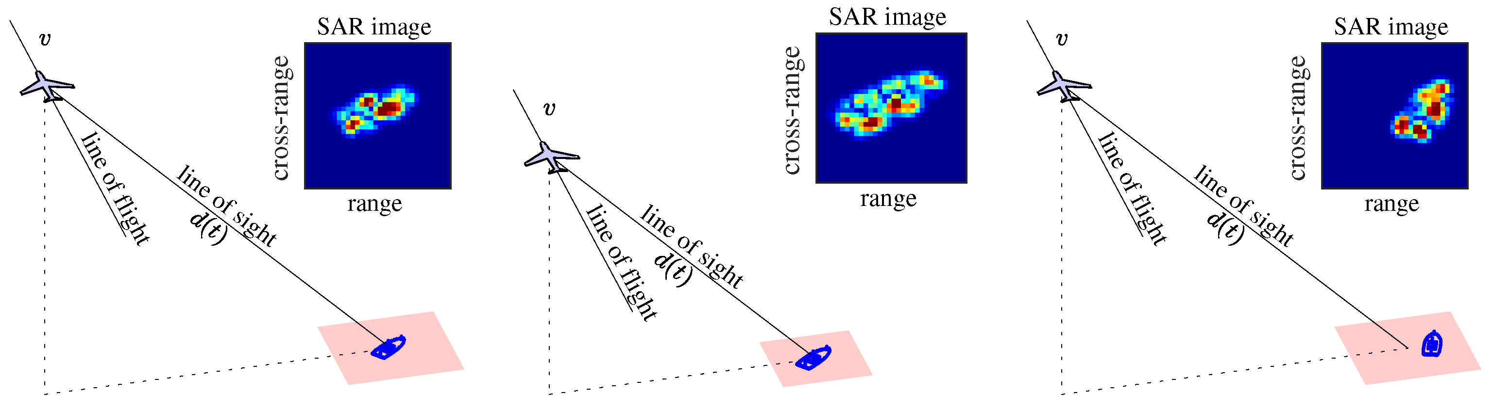
2.1. Basic SAR Principles

A radar image is obtained by transmitting repeated pulses and processing the echoes returned from the target [26,27,28,29,30,31,32]. A common choice for the pulse is a linear-frequency-modulated continuous-wave (LFM-CW) signal, transmitted in the form of a series of chirps. The received signal, which is scattered from a target, is delayed and changed in amplitude as compared to the transmitted signal, containing in that way the information about the target position and reflectivity. The received signal from an elementary (a point) scatter, after an appropriate mixing with the transmitted signal, demodulation, compensation, and residual video phase filtering is of the form [1]

$$\begin{array}{c}\hfill S(m,t)=\sigma exp\left(j{\omega }_0\frac{2d\left(t\right)}{c}\right)exp\left(-j2\pi \frac{B(t - m{T}_r)}{T_r}\frac{2d\left(t\right)}{c}\right)\end{array}$$

(1)

where $\sigma$ is the reflection coefficient of the scattering point, ${\omega }_0$ is the radar operating frequency, $exp(j{\omega }_0\frac{2d\left(t\right)}{c})$ is the scattering phase, and $exp(-j2\pi \frac{B}{T_r}(t-m{T}_r)\frac{2d\left(t\right)}{c})$ describes the phase variation due to the varying distance. The transmission and receiving procedure is repeated every $T_r$ second (the pulse repetition interval—PRI).

In SAR imaging, the radar platform movement is crucial in producing a high-resolution image. Therefore, SAR systems are based on a pulsed radar installed on a platform with a forward movement. The distance between the radar moving at a constant velocity v and a point target on the ground can be described as [2]

$$\begin{array}{c}\hfill d\left(t\right)=\sqrt{d_0^2+{\left(vt\right)}^2}\end{array}$$

(2)

where $t=0$ is the time of closest approach when the distance is minimum as $d\left(0\right)=d_0$. Assume M pulses are transmitted and N range cells are inside a pulse interval, $t=n{T}_s$. The received echo signal can form an $M\times N$ data matrix of complex samples. The column dimension corresponds to the range direction. Note, the radar acquires a range line in each PRI thus forming the row dimension of the data matrix, termed the azimuth direction. In the case of multi-point targets, the superposition principle applies. Therefore, the raw SAR data are the echoes from the illuminated scene (of multiple points or even continuous targets) sampled both in the range direction and azimuth direction.

Different from optical sensors, however, raw SAR data do not provide any visible information on the scene [1]. It is only after basic SAR processing steps that an image is obtained. In a very simplified way, the complete processing can be understood as two separate matched filter operations along with the range and azimuth dimensions; instead of performing a convolution in the time domain, multiplication in the frequency domain is adopted due to the much lower computational load. The first step is to compress the transmitted chirp signals to a short pulse. Azimuth compression follows the same basic reasoning; that is, the signal is convolved with its reference function, which is the complex conjugate of the response expected from a point target on the ground. The SAR image is efficiently calculated using, for example, the two-dimensional fast Fourier transform (FFT) codes [33].

To know a target or scene for analysis, detection, or classification, it is desirable to have its SAR image acquired from different positions [34,35]. Different relative viewing angles (resulting from changes in flight direction or target movement in different revisits) result in a kind of target rotation in SAR images. The radar revisits could be also conducted from different distances to the target or the target could move between revisits resulting in a kind of target shifting and/or scaling in the SAR image. These kinds of target changes in radar images will be referred to as properties of the target, as illustrated in Figure 1. In some cases, numerous revisits or observations may be expensive or in some hostile or unique environments even not possible. Then, it would be of interest to use the available set of data and try to synthesize new possible images, preferably with controlled properties, defined by, for example, different rotations, translation, and scaling that would at the same time fully correspond to the existing data. To this aim, we will present and apply the GAN and InfoGAN.

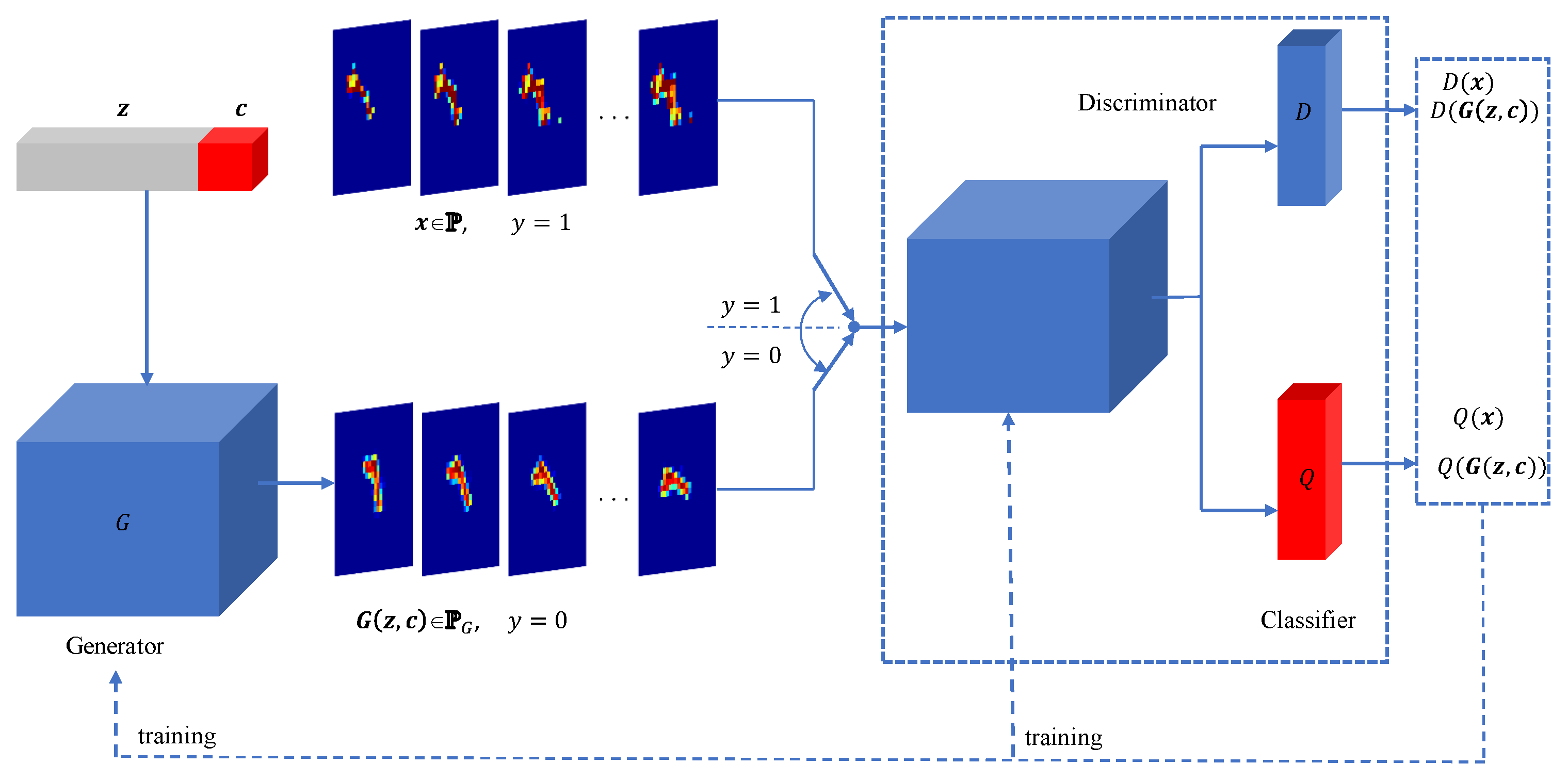
2.2. GAN and InfoGAN

The main task of a generative adversarial network is to train a transposed neural network to produce images that match real images ${\mathbf{x}}_n$ from a set $\mathbb{P}$ [12,36]. It means that the GAN learns a generator (transposed convolution neural network), denoted by G, to synthesize images close to $\mathbb{P}$ by feeding the generator with a noise vector $\mathbf{z}$, commonly Gaussian or uniformly distributed. $\mathbf{G}\left(\mathbf{z}\right)$ denotes an image from a set of generated images, ${\mathbb{P}}_G$. The generator is trained against an adversarial discriminator network, D, whose structure corresponds to a convolution neural network with the aim to distinguish (discriminate the cases) if the sample image as the input to the discriminator is from the true dataset of images, $\mathbb{P}$, or from the generator-produced set of images, ${\mathbb{P}}_G$. The basic structure of a GAN is included in Figure 2.

After both networks, the generator and the discriminator, are initialized by random weights, the training process is defined based on the loss function. First, we will consider the discriminator only. At its input, we have an image (as is common for a convolutional neural network), either a sample image $\mathbf{x}$ from the set of real data, $\mathbb{P}$, or a synthesized image, $\mathbf{G}\left(\mathbf{z}\right)$, produced by the generator with a random input noise, $\mathbf{z}$. The output of the discriminator is a scalar denoted by $D(·)$. It is either $D\left(\mathbf{x}\right)$ or $D\left(\mathbf{G}\right(\mathbf{z}\left)\right)$. The output value of the discriminator is normalized such that $0\le D\left(\mathbf{x}\right),D\left(\mathbf{G}\right(\mathbf{z}\left)\right)\le 1$. The aim of the discriminator is to discriminate the cases when the input is (i) a real image from $\mathbb{P}\left(\mathbf{x}\right)$ or (ii) a generated “fake” (synthesized) image $\mathbf{G}\left(\mathbf{z}\right)$, by learning to produce the output values $D\left(\mathbf{x}\right)$ close to 1 and the values $D\left(\mathbf{G}\right(\mathbf{z}\left)\right)$ close to 0. The target signal, which will be used during the supervised learning, will be denoted by $y_{\mathbf{x}}$. It assumes that the values are as follows:

• $y_{\mathbf{x}}=1$ if the input to the discriminator is a real image $\mathbf{x}$ from the set $\mathbb{P}\left(\mathbf{x}\right)$;
• $y_{\mathbf{x}}=0$ if the input to the discriminator is a synthesized image, $G\left(\mathbf{z}\right)$, being output from the generator.

The value of the target signal, $y_{\mathbf{x}}$, is provided at the output of the discriminator as a reference signal for the loss function calculation during the training process. A simple loss function could be in a quadratic form

$$\mathcal{L}\left(D\right)=y_{\mathbf{x}}{D}^2\left(\mathbf{x}\right)+(1-y_{\mathbf{x}}){(1-D\left(\mathbf{G}\left(\mathbf{z}\right)\right))}^2.$$

(3)

This function assumes only one of two values $\mathcal{L}\in \{D^2\left(\mathbf{x}\right),(1-D{\left(\mathbf{G}\left(\mathbf{z}\right)\right)}^2\}$. Since $0\le D\left(\mathbf{x}\right),D\left(G\right(\mathbf{z}\left)\right)\le 1$, the loss function will reach its maximum value $\mathcal{L}\left(D\right)=1$ for any input to the discriminator, either $\mathbf{x}$ or $\mathbf{G}\left(\mathbf{x}\right)$, if $D\left(\mathbf{x}\right)=1$ and $D\left(G\right(\mathbf{z}\left)\right)=0$. Therefore, by maximizing the loss function $\mathcal{L}\left(D\right)$, we can achieve the ideal discriminator performance.

In a vanilla GAN, the cross-entropy form of the loss function is used (with the same aim and the same qualitative analysis as in the quadratic loss function) [37]. The cross-entropy form of the loss function is defined by $y_{\mathbf{x}}logD\left(\mathbf{x}\right)+(1-y_{\mathbf{x}})log(1-D\left(\mathbf{G}\left(\mathbf{z}\right)\right)$, with the learning process for the discriminator neural network defined as

$$\underset{D}{max}\mathcal{L}\left(D\right)=\underset{D}{max}\{y_{\mathbf{x}}logD\left(\mathbf{x}\right)+(1-y_{\mathbf{x}})log(1-D\left(\mathbf{G}\left(\mathbf{z}\right)\right)\}.$$

(4)

It is easy to conclude that, for $0\le D\left(\mathbf{x}\right),D\left(G\right(\mathbf{z}\left)\right)\le 1$, this loss function achieves its maximum $\mathcal{L}\left(D\right)=0$ when $D\left(\mathbf{x}\right)=1$ and $D\left(G\right(\mathbf{z}\left)\right)=0$.

The maximization of the cross-entropy loss function is commonly conducted over a set (mini-batch) of input real images, ${\mathbf{x}}_1$, ${\mathbf{x}}_2$,…, ${\mathbf{x}}_m$, and generated images, $\mathbf{G}\left({\mathbf{z}}_1\right),\mathbf{G}\left({\mathbf{z}}_2\right),\dots ,\mathbf{G}\left({\mathbf{z}}_m\right)$. The expression for the cross-entropy loss function will also be simplified by omitting $y_{{\mathbf{x}}_i}$. Namely, it will be assumed that the input to the discriminator is fed by alternating ${\mathbf{x}}_1$ and $\mathbf{G}\left({\mathbf{z}}_1\right)$, then ${\mathbf{x}}_2$ and $\mathbf{G}\left({\mathbf{z}}_2\right)$, and so on in succession until ${\mathbf{x}}_m$ and $\mathbf{G}\left({\mathbf{z}}_m\right)$. In this way, we may write two loss function terms: (i) $logD\left({\mathbf{x}}_i\right)$ for ${\mathbf{x}}_i$ and (ii) $log(1-D\left(\mathbf{G}\left({\mathbf{z}}_i\right)\right))$ for $\mathbf{G}\left({\mathbf{z}}_i\right)$ as $logD\left({\mathbf{x}}_i\right)+log(1-D\left(\mathbf{G}\left({\mathbf{z}}_i\right)\right))$, for each $i=1,2,\cdots ,m$. The mean value over $2m$ images (m real images and m generated images) is then defined by

$$\underset{D}{max}\mathcal{L}\left(D\right)=\underset{D}{max}\frac{1}{m}\sum _{i=1}^m\left(logD\left({\mathbf{x}}_i\right)+log(1-D\left(\mathbf{G}\left({\mathbf{z}}_i\right)\right))\right).$$

(5)

After the discriminator is trained (in the first cycle) based on the loss function (5), its weights are frozen and the generator network is now trained for this cycle. Since the generator does not have any knowledge about the real images, the part $logD\left(\mathbf{x}\right)$ is not used in the loss function for the generator weight training (only generated images are used, when $y_{{\mathbf{x}}_i}=0$). The aim of the generator is to produce images as similar to those from the set $\mathbb{P}\left(\mathbf{x}\right)$ as possible. Within the loss function framework, this aim will be achieved if the generator can close the gap between the discriminator output values $D\left(\mathbf{x}\right)$ and $D\left(\mathbf{G}\right(\mathbf{x}\left)\right)$ as much as possible. Since it can not change $D\left(\mathbf{x}\right)$, this should be conducted by increasing the value of $D\left(\mathbf{G}\right(\mathbf{x}\left)\right)$ toward 1 or, in other words, by making the new loss function $\mathcal{L}\left(G\right)=log(1-D(\mathbf{G}\left(\mathbf{z}\right)\left)\right)$ as small as possible, that is (within the same mini-batch), find

$$\underset{G}{min}\{\frac{1}{m}\sum _{i=1}^{m}log(1-D\left(\mathbf{G}\left({\mathbf{z}}_i\right)\right))\}.$$

(6)

After the generator is trained in this way (in the first cycle), its weights are frozen and the discriminator network is trained again within the second cycle. These cycles are continued for a defined number of echoes when the GAN is assumed to be fully trained. In the ideal case, after the training is finished, the discriminator will not be able to discriminate the real and the synthesized images from the generator, meaning it will produce the output $D\left(\mathbf{x}\right)=D\left(G\right(\mathbf{z}\left)\right)=1/2$ and the loss function value of form (5) will be $\mathcal{L}\left(D\right)=2log(1/2)=-4$.

The combined loss function of GAN for both the discriminator and the generator can be summarized by the following expression:

$$\begin{array}{cc}\hfill \underset{G}{min}\underset{D}{max}\mathcal{L}(G,D)=& {\mathbb{E}}_{\mathbf{x}}\{logD\left(\mathbf{x}\right)\}\hfill \\ \hfill & +{\mathbb{E}}_{\mathbf{z}}\{log(1-D\left(\mathbf{G}\left(\mathbf{z}\right)\right))\}.\hfill \end{array}$$

(7)

It is clear from (7) that no restrictions are imposed on the input noise data; thus, the properties are highly entangled in generated images. To generate images with semantically meaningful properties, the InfoGAN introduces latent codes, $\mathbf{c}=[c_1,c_2,\cdots ,c_n]$, and a classifier, Q, with the same architecture sharing the trainable parameters with the discriminator. The purpose of classifier is to maximize the mutual information $I(\mathbf{c};\mathbf{G}(\mathbf{z},\mathbf{c}\left)\right)$ between $\mathbf{c}$ and $\mathbf{G}(\mathbf{z},\mathbf{c})$, defined as follows:

$$\begin{array}{c}\hfill I(\mathbf{c};\mathbf{G}(\mathbf{z},\mathbf{c}\left)\right)=H\left(\mathbf{c}\right)-H\left(\mathbf{c}\right|(\mathbf{z},\mathbf{c}))\end{array}$$

(8)

where $H\left(\mathbf{c}\right)=-{\sum }_{i}p\left(c_i\right)log\left(p\left(c_i\right)\right)$ is the entropy of $\mathbf{c}=[c_1,c_2,\cdots ,c_n]$. The mutual information $I(\mathbf{c};\mathbf{G}(\mathbf{z},\mathbf{c}\left)\right)$ means that if $\mathbf{c}$ and $\mathbf{G}(\mathbf{z},\mathbf{c})$ are independent, then $I(\mathbf{c};\mathbf{G}(\mathbf{z},\mathbf{c}\left)\right)=0$, because knowing c reveals nothing about the $\mathbf{G}(\mathbf{z},\mathbf{c})$ (degraded to the classic GAN); by contrast, if $\mathbf{c}$ and $\mathbf{G}(\mathbf{z},\mathbf{c})$ are strongly related, then maximal mutual information is attained. It means that the information in the latent code $\mathbf{c}$ should not be lost in the generation process. Hence, the information-regularized loss function is as follows:

$$\begin{array}{cc}\hfill \underset{G}{min}\underset{D}{max}{\mathcal{L}}_I(G,D)=& {\mathbb{E}}_{\mathbf{x}}\{logD\left(\mathbf{x}\right)\}+{\mathbb{E}}_{\mathbf{z}}\{log(1-D\left(\mathbf{G}\left(\mathbf{z}\right)\right))\}\hfill \\ \hfill & + \lambda I(\mathbf{c};\mathbf{G}(\mathbf{z},\mathbf{c}\left)\right).\hfill \end{array}$$

(9)

Figure 2 shows the architecture of an InfoGAN. To show the difference between the GAN and InfoGAN vividly, we particularly provide some generated images from two networks in Figure 3. Here, we set one latent code, $c_1$, in the InfoGAN and show the generated images corresponding to 25 values of $c_1$ uniformly distributed within $[-1$, $1]$. We further utilize a commonly used quantitative measurement, i.e., Fréchet Inception Distance (FID) [38,39], to evaluate the quality of generated SAR images produced by the GAN and InfoGAN, respectively. The FID measures similarity between two sets of images (${\mathbf{z}}_1$ and ${\mathbf{z}}_2$), and it is defined as follows:

$$\begin{array}{c}\hfill \mathrm{FID}({\mathbf{z}}_1,{\mathbf{z}}_2)={\parallel {\mu }_{z_1}-{\mu }_{z_2}\parallel }_2^2+\mathrm{Tr}[{\mathrm{\Psi }}_{z_1}+{\mathrm{\Psi }}_{z_2}-2{\left({\mathrm{\Psi }}_{z_1}{\mathrm{\Psi }}_{z_2}\right)}^{\frac{1}{2}}],\end{array}$$

(10)

where ${\parallel \parallel }_2^2$ denotes the squared $L_2$ norm, $\mu$ is the mean of a dataset, $Tr$ denotes the trace of a matrix, ${\mathrm{\Psi }}_{z_1}$ and ${\mathrm{\Psi }}_{z_2}$ refer to the covariance matrices of ${\mathbf{z}}_1$ and ${\mathbf{z}}_2$, respectively. Hence, a small value of FID means a high similarity between two datasets ($FID=0$ only when ${\mathbf{z}}_1$ is completely the same as ${\mathbf{z}}_2$). We computed the $FID$ between SAR images generated by two GAN models and training SAR images, as shown in

Table 1. The FID of images generated by two GANs and training images.

Model	FID
GAN	18.74
InfoGAN	17.59

. It is clear that the images generated by two GANs are almost equally similar to the training images (slightly favoring the InfoGAN), while only the InfoGAN focuses on property manipulation using latent codes.

3. Methodology

Next, we will consider SAR images of the target taken with various setups and relate them to the latent codes in the InfoGAN. The aim is to train the InfoGAN to synthesize available images with various target properties and to produce new ones by changing latent codes. This process could be controlled by relating the latent codes to the SAR image transformations. Cases with one and two properties will be considered. In the analysis of one property, we will use one or two latent codes, while in the case of two-properties two latent codes are used.

3.1. Property Measurement

When the radar illuminates a target (for example, a vehicle, a ship, or any other object of interest) in two different visits, SAR images may differ due to different viewing angles, target maneuvering, or different distances between the radar and the target in these two illuminations. The changes in the radar image can be described by a rotation (with possible changes in the reflectivity or visibility of some scatters in the target). Other possible change in the SAR image results from the possible distance change between the radar and the target and may be described by a scaling of the target in SAR images (with possible changes in the radar image structures due to the fusing or separation of close scatters due to the resolution values). This will be referred to as the scaling property. In addition, the target relative position can be changed in two different illuminations, causing shifts in the radar image.

To quantify these properties of radar images, we should introduce their relative measures with respect to one SAR image, assumed to be the reference image. To this aim, we will use the cross-correlation function to evaluate the similarity between two images [40]. Assume $\mathbf{X}$ and $\mathbf{Y}$ are two images of the same size, $N\times N$. The cross-correlation between these two images, $r(\mathbf{X},\mathbf{Y})$, is defined as

$$\begin{array}{cc}\hfill r(\mathbf{X},\mathbf{Y})& =\frac{{\sum }_i{\sum }_j(X(i,j)-\overline{X}){\sum }_i{\sum }_j(Y(i,j)-\overline{Y})}{\sqrt{{\sum }_i{\sum }_j{(X(i,j)-\overline{X})}^2}\sqrt{{\sum }_i{\sum }_j{(Y(i,j)-\overline{Y})}^2}}\hfill \end{array}$$

(11)

$$\begin{array}{cc}\hfill \overline{X}& =\frac{1}{N^2}\sum _i\sum _{j}X(i,j),\overline{Y}=\frac{1}{N^2}\sum _i\sum _{j}Y(i,j)\hfill \end{array}$$

(12)

where $\overline{X}$ and $\overline{Y}$ denote the mean of images $\mathbf{X}$ and $\mathbf{Y}$, and the denominator normalizes the cross-correlation to the range from 0 to 1. The summation range is from 1 to N for all sums in (11) and (12). It can be observed that $r(\mathbf{X},\mathbf{Y})$ will be 1 if $\mathbf{X}=\mathbf{Y}$, and $r(\mathbf{X},\mathbf{Y})$ will assume a value smaller than 1 if $\mathbf{X}$ is becoming more different from $\mathbf{Y}$.

If we want to use cross-correlation to measure the translation of a target ${\mathbf{I}}_j$ with respect to the reference image ${\mathbf{I}}_0$, then we will perform the translation operation of the reference image ${\mathbf{I}}_0$ for different $d_x$ with steps $\mathrm{\Delta }{d}_x$ and $d_y$ with steps $\mathrm{\Delta }{d}_y$, denoted by ${\mathcal{T}}_{\delta }\left\{{\mathbf{I}}_0\right\}$, and find the resulting translation parameter as the position $d_x$, $d_y$ when the maximum of the function $r({\mathcal{T}}_{\delta }\left\{{\mathbf{I}}_0\right\},{\mathbf{I}}_j)$ is found

$$\begin{array}{c}\hfill {\delta }_S\left(j\right)=arg\underset{\delta }{max}\left\{r({\mathcal{T}}_{\delta }\left\{{\mathbf{I}}_0\right\},{\mathbf{I}}_j)\right\},\end{array}$$

(13)

where ${\delta }_S$ is, in general, a vector, with corresponding shifts in the direction of the range and cross-range [6].

Similarly, we say that the original image is rotated for ${\delta }_R$ when the maximum of the cross-correlation between the reference image, rotated for an angle ${\delta }_R$, and the considered image ${\mathbf{I}}_j$ is found, that is

$$\begin{array}{c}\hfill {\delta }_R\left(j\right)=arg\underset{\delta }{max}\left\{r({\mathcal{R}}_{\delta }\left\{{\mathbf{I}}_0\right\},{\mathbf{I}}_j)\right\},\end{array}$$

(14)

where now ${\mathcal{R}}_{\delta }\left\{{\mathbf{I}}_0\right\}$ denotes the reference image rotated for an angle ${\delta }_R\left(j\right)$. The rotated and reference image may differ in reflectivity, meaning that the maximum value of the cross-correlation will not be equal to one. To reduce the influence of the variations in the reflectivity during the rotations, we can introduce a threshold (limiting) or even consider only the support functions (the support function of an image assumes value 0 where the image is 0 or close to 0 and 1 otherwise) of the considered objects. The rotation parameter is then calculated as

$$\begin{array}{c}\hfill {\delta }_R\left(j\right)=arg\underset{\delta }{max}\left\{r({\mathcal{R}}_{\delta }\left\{{\mathbf{H}}_T\left\{{\mathbf{I}}_0\right\}\right\},{\mathbf{H}}_T\left\{{\mathbf{I}}_j\right\})\right\},\end{array}$$

(15)

where ${\mathbf{H}}_T\left\{\mathbf{I}\right\}$ denotes the limited version of the image $\mathbf{I}$, with a threshold T, that is

$$\begin{array}{c}\hfill {\mathbf{H}}_T\left\{I(i,j)\right\}=\left\{\begin{array}{cc}I(i,j)\hfill & \mathrm{for}I(i,j)\le T\hfill \\ T\hfill & \mathrm{for}I(i,j)>T.\hfill \end{array}\right.\end{array}$$

(16)

Finally, the scaling property is defined in the same way, as the position of the maximum correlation between the considered image ${\mathbf{I}}_j$ and the scaled reference image ${\mathcal{S}}_{\delta }\left\{{\mathbf{I}}_0\right\}$ for a scaling parameter $\delta$, that is

$$\begin{array}{c}\hfill {\delta }_A\left(j\right)=arg\underset{\delta }{max}\left\{r({\mathcal{S}}_{\delta }\left\{{\mathbf{I}}_0\right\},{\mathbf{I}}_j)\right\}.\end{array}$$

(17)

After we introduced measures of various mage transformations, we are now ready to relate them with latent codes in the InfoGAN.

3.2. Relation of the Properties and Latent Codes

As mentioned above, we have three collocations of property–latent code pairs, i.e., one property—one latent code, one property—two latent codes, and two properties—two latent codes. It is necessary to clarify that the cross-correlation will not be sensitive enough to gauge each individual property if we combine three properties together. To simplify the issue and avoid entanglement among latent codes, we only consider one latent code and two latent codes. It is the reason why such three collocations are set in our experiments.

One property—one latent code: Next, we assume that the InfoGAN is trained with P real SAR images when one of the considered properties (for example, the relative angle of a target with respect to the radar direction) changes. After the learning process, the InfoGAN is able to synthesize the corresponding SAR images, in an ideal case the same as the real original images, with the latent code ${\mathbf{c}}_1$, being related to the property change in the particular SAR images. After the learning process has finished, we generate a new set of K latent code values ${\mathbf{c}}_1={[c_1\left(1\right),c_1\left(2\right),\cdots ,c_1\left(K\right)]}^T$. Then, a set of images is generated using the values $c_1\left(k\right)$, $k=1,2,\cdots ,K$, and random input noises ${\mathbf{z}}_k$. The obtained images are denoted by

$$\begin{array}{c}\hfill {\mathbf{I}}_k=\mathbf{G}({\mathbf{z}}_k,c_1\left(k\right)),k=1,2,\cdots ,K.\end{array}$$

(18)

Then, we use one of the measures (13), (15), or (17) to calculate the measure of properties for each synthesized SAR image from the set. The relative measure of the rotation with respect to the reference image ${\mathbf{I}}_0$ is calculated using

$$\begin{array}{c}\hfill \begin{array}{cc}\hfill {\delta }_R\left(1\right)& =argmax\left\{r({\mathcal{R}}_{\delta }\left\{{\mathbf{H}}_T\left\{{\mathbf{I}}_0\right\}\right\},{\mathbf{H}}_T\left\{{\mathbf{I}}_1\right\})\right\}\hfill \\ \hfill {\delta }_R\left(2\right)& =argmax\left\{r({\mathcal{R}}_{\delta }\left\{{\mathbf{H}}_T\left\{{\mathbf{I}}_0\right\}\right\},{\mathbf{H}}_T\left\{{\mathbf{I}}_2\right\})\right\}\hfill \\ \hfill & \cdots \hfill \\ \hfill {\delta }_R\left(K\right)& =argmax\left\{r({\mathcal{R}}_{\delta }\left\{{\mathbf{H}}_T\left\{{\mathbf{I}}_0\right\}\right\},{\mathbf{H}}_T\left\{{\mathbf{I}}_K\right\})\right\}\hfill \end{array}\end{array}$$

(19)

(a) Linear model: For the rough analysis, we consider a linear model for the approximation of the obtained measure of rotation and the latent code used to produce the corresponding image

$$\begin{array}{c}\hfill {\widehat{\delta }}_R\left(k\right)=v_1{c}_1\left(k\right)+v_0,k=1,2,\cdots ,K.\end{array}$$

(20)

where $v_0$ and $v_1$ are two unknown parameters. To estimate them, we can write a matrix form of these equations

$$\begin{array}{c}\hfill {\widehat{\delta }}_R=\left[\begin{array}{c}{\widehat{\delta }}_R\left(1\right)\\ {\widehat{\delta }}_R\left(2\right)\\ ⋮\\ {\widehat{\delta }}_R\left(K\right)\end{array}\right]=\left[\begin{array}{cc}{c}_1\left(1\right)& 1\\ c_1\left(2\right)& 1\\ ⋮\\ c_1\left(K\right)& 1\end{array}\right]\left[\begin{array}{c}{v}_1\\ v_0\end{array}\right]=\mathbf{A}\mathbf{V},\end{array}$$

(21)

where $\mathbf{A}$ is a matrix with a column of latent code and a column of 1, and $\mathbf{V}={[v_1,v_0]}^T$.

Now, we can obtain the optimal parameters $v_0$ and $v_1$ by optimizing the following equation:

$$\begin{array}{c}\hfill \mathbf{V}=argmin\parallel {\delta }_R-{\hat{\delta }}_R{\parallel }_2^2\end{array}$$

(22)

where ${\delta }_R$ represents the vector column of the values obtained from (19) and ${\widehat{\delta }}_R$ is given by (21). The solution is

$$\begin{array}{c}\hfill \mathbf{V}={\left({\mathbf{A}}^T\mathbf{A}\right)}^{-1}{\mathbf{A}}^T{\widehat{\delta }}_R.\end{array}$$

(23)

After the relation between the considered property (rotation) and latent code is established, we can now use it to calculate a satisfying value of the latent code $c_1$ to produce a SAR image, ${\mathbf{I}}_d$, for any desired rotation angle ${\delta }_{Rd}$,

$$\begin{array}{c}\hfill c_1=\frac{{\delta }_{Rd}-v_0}{v_1},\end{array}$$

(24)

as ${\mathbf{I}}_d=\mathbf{G}(\mathbf{z},c_1)$.

The linear model is very simple; however, as will be seen from the experiments, it can be used as a rough model only. Namely, the true relation between rotation and latent code is nonlinear, governed by the nonlinearity in the InfoGAN.

(b) Nonlinear model: From the experiments, we concluded that a general form of a function (following the sigmoid function at the output of the neural network) is quite an appropriate model for the relation between the physical properties of the SAR image and the latent codes. The sigmoid follows the tanh function. A nonlinear model of, for example, rotation, with one latent code ${\mathbf{c}}_1$ could be written as follows:

$$\begin{array}{c}\hfill {\widehat{\delta }}_R\left(k\right)=v_{3}tanh(v_1{c}_1\left(k\right)+v_2)+v_0,k=1,2,\cdots ,K.\end{array}$$

(25)

The solution to the minimization problem (22) cannot be obtained in an analytic form in this case. However, the tools for numerical solutions to this problem are well developed in all programming environments. Therefore, we may say that the values of $\mathbf{V}={[v_0,v_1,v_2,v_3]}^T$ can be obtained from a set of k nonlinear equations in (25). After the model coefficients, $\mathbf{V}$, are found, we can again easily find a latent code $c_1$ to generate a SAR image, ${\mathbf{I}}_d$, with a desired parameter ${\delta }_{Rd}$, as

$$\begin{array}{c}\hfill c_1=\frac{1}{v_1}{tanh}^{-1}\left(\frac{{\delta }_{Rd}}{v_3}-v_0\right)-v_2.\end{array}$$

(26)

as ${\mathbf{I}}_d=\mathbf{G}(\mathbf{z},c_1)$.

One property—two latent codes: In SAR images, after the basic property change, we can expect other changes to occur as well (such as changes in the reflectivity and visibility of scatters). This means that, even with one geometric property change, we may still use more than one latent code. Now, we extend the analysis to two latent codes $c_1$ and $c_2$. The linear model for a two-latent-code space can be expressed as

$$\begin{array}{c}\hfill {\widehat{\delta }}_R(k_1,k_2)=v_2{c}_2\left(k_2\right)+v_1{c}_1\left(k_1\right)+v_0,k_1,k_2=1,2,\cdots ,K.\end{array}$$

If we form a stacked column vector ${\widehat{\delta }}_R$ with $K^2$ elements ${\widehat{\delta }}_R(k_1,k_2)$, a $K^2\times 3$ matrix $\mathbf{A}$ with rows $[c_2\left(k_2\right),c_1\left(k_1\right),1]$, and the column vector of unknown coefficients $\mathbf{V}={[v_2,v_1,v_0]}^T$, then the solution is again obtained in the form $\mathbf{V}={\left({\mathbf{A}}^T\mathbf{A}\right)}^{-1}{\mathbf{A}}^T{\widehat{\delta }}_R$.

In this case, the latent code values for a given property, for example, rotation ${\delta }_{Rd}$, are not unique since all combinations of the latent codes are along the line

$$v_2{c}_2+v_1{c}_1=v_0-{\delta }_{Rd}$$

(27)

in the $c_1$-$c_2$ plane, which will produce the same desired rotation ${\delta }_{Rd}$. The desired rotation can be obtained by fixing one latent code, $c_1$ or $c_2$, and calculating the other latent code value.

For two latent codes, the nonlinear model is of the form

$$\begin{array}{c}{\widehat{\delta }}_R(k_1,k_2)=v_{4}tanh(v_1{c}_1\left(k_1\right)+v_2{c}_2\left(k_2\right)+v_3)+v_0,\\ k_1,k_2=1,2,\cdots ,K\end{array}$$

(28)

The optimization of parameters $v_4$, $v_3$, $v_2$, $v_1$, and $v_0$ is conducted using common nonlinear fitting tools. The line for a desired ${\delta }_{Rd}$ is obtained in the form

$$\begin{array}{c}\hfill v_1{c}_1+v_2{c}_2={tanh}^{-1}\left(\frac{{\delta }_{Rd}-v_0}{v_4}\right).\end{array}$$

(29)

Again, a desired ${\delta }_{Rd}$ can be achieved with all pairs of $(c_1,c_2)$ on the previous line.

In the nonlinear model, we further introduce a quadratic term in the argument of the tanh function as

$$\begin{array}{c}{\delta }_R(k_1,k_2)=v_{7}tanh(P_R(c_1\left(k\right),c_2\left(k_2\right))+v_0,\\ k_1,k_2=1,2,\cdots ,K.\end{array}$$

(30)

where $P_R(c_1\left(k\right),c_2\left(k_2\right))=v_1{c}_1^2\left(k_1\right)+v_2{c}_2^2\left(k_2\right)+v_3{c}_1\left(k_1\right)c_2\left(k_2\right)+v_4{c}_1\left(k\right),+v_5{c}_2\left(k\right)+v_6$, $k_1,k_2=1,2,\cdots ,K$. For a desired ${\delta }_{Rd}$, ($c_1$, $c_2$) should be satisfied by the following relation

$$\begin{array}{c}\hfill P_R(c_1,c_2)={tanh}^{-1}\left(\frac{{\delta }_{Rd-v_0}}{v_7}\right)\end{array}$$

(31)

meaning all combinations of the latent codes are along a quadratic form line. Namely, (31) is a general quadratic equation, producing conic sections (circles, ellipses, parabolas, and hyperbolas) in the $c_1$-$c_2$ plane, depending on the specific parameter $v_0,v_1,v_2,\cdots ,v_7$ values.

Two properties—two latent codes: For a simultaneous change in two properties, we will use two codes and a nonlinear model. In the nonlinear model, we will use a linear argument form of the tanh function and a quadratic argument of this function. In the case of the linear argument, we will use the model

$$\begin{array}{cc}\hfill {\delta }_R(k_1,k_2)& =v_{4}tanh(v_1{c}_1\left(k_1\right)+v_2{c}_2\left(k_2\right)+v_3)+v_0,\hfill \\ \hfill {\delta }_S(k_1,k_2)& =v_{9}tanh(v_6{c}_1\left(k_1\right)+v_7{c}_2\left(k_2\right)+v_8)+v_5,\hfill \end{array}$$

(32)

The quadratic argument model is of the form

$$\begin{array}{cc}\hfill {\delta }_R(k_1,k_2)& =v_{7}tanh(P_R(c_1\left(k\right),c_2\left(k_2\right))+v_0,\hfill \end{array}$$

(33)

$$\begin{array}{cc}\hfill {\delta }_S(k_1,k_2)& =v_{15}tanh(P_S(c_1\left(k\right),c_2\left(k_2\right))+v_8,\hfill \\ \hfill & k_1,k_2=1,2,\cdots ,K,\hfill \end{array}$$

(34)

where the polynomial arguments for the two properties are defined by

$$\begin{array}{cc}\hfill P_R(c_1\left(k_1\right),c_2\left(k_2\right))=& v_1{c}_1^2\left(k_1\right)+v_2{c}_2^2\left(k_2\right)+v_3{c}_1\left(k_1\right)c_2\left(k_2\right)\hfill \\ \hfill & +v_4{c}_1\left(k_1\right)+v_5\left(c\left(k2\right)\right)+v_6,\hfill \end{array}$$

(35)

$$\begin{array}{cc}\hfill P_S(c_1\left(k_1\right),c_2\left(k_2\right))=& v_9{c}_1^2\left(k_1\right)+v_{10}{c}_2^2\left(k_2\right)+v_{11}{c}_1\left(k_1\right)c_2\left(k_2\right)\hfill \\ \hfill & +v_{12}{c}_1\left(k_1\right)+v_{13}\left(c\left(k2\right)\right)+v_{14},\hfill \end{array}$$

(36)

for $k_1,k_2=1,2,\cdots ,K$. These two systems are independently solved for the corresponding sets of coefficients in the model.

In this case, the desired SAR image is generated at the intersection of the lines producing the desired rotation, ${\delta }_{Rd}$, and scaling, ${\delta }_{Sd}$, since for each of them we get the corresponding lines as in (29) and (31).

All the previous setups will be illustrated and explained in detail in the next section dealing with experimental results. It is worth noting that motion error is a key problem in the practical application of SAR image formation [41]. Specifically, SAR images will be unfocused or blurred if there are motion errors. Here, we clarify that the relation between motion error and latent codes is beyond the scope of this paper because (1) motion error is a complex issue that could be too difficult for one or two latent codes to capture its physical regulation; (2) motion error is also difficult to gauge numerically while the objective of this paper is to provide a numerical interpretation of the relation between properties (i.e., the properties should be gauged numerically and easily) and latent codes. Nonetheless, it is still an important issue worth studying in the future and could be feasible to interpret by introducing more smart estimators and regularization.

4. Experiments

Dataset: In our experiments, four kinds of datasets are utilized as shown in Figure 4 and

Table 2. The detailed information of each dataset.

Dataset	Property	Spatial Size	Number of Samples
simulated	rotation	$28\times 28$	$13/121$
semi-simulated	rotation	$28\times 28$	601
semi-simulated	translation	$28\times 28$	151
semi-simulated	scaling	$28\times 28$	301
semi-simulated	rotation and translation	$28\times 28$	3721
semi-simulated	rotation and scaling	$28\times 28$	1891
semi-simulated	translation and scaling	$28\times 28$	3751
real without background	rotation	$28\times 28$	60
real with background	rotation	$28\times 28$	60

:

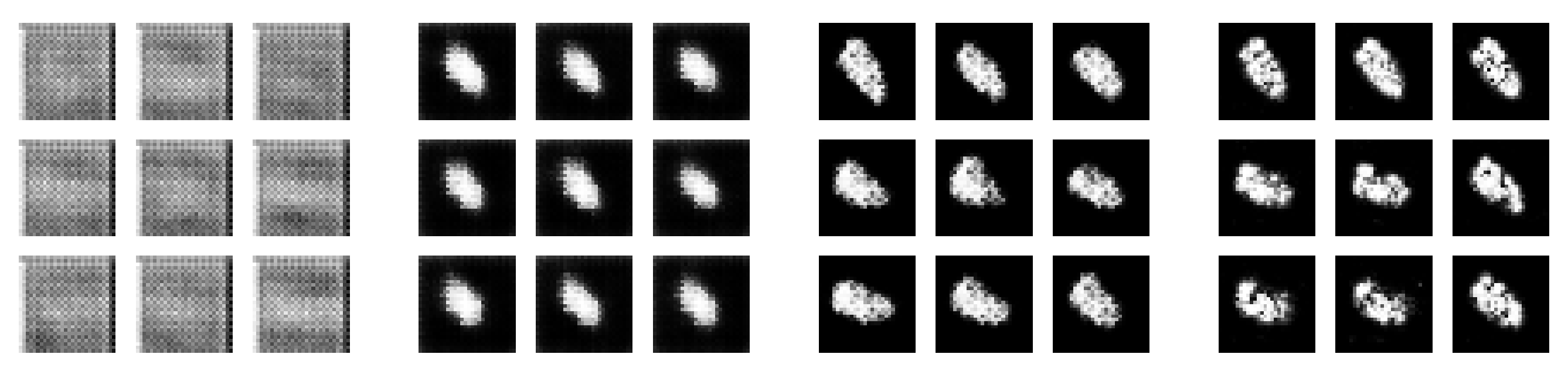
• Simulated SAR images: This dataset contains SAR images produced by a simulation model, retaining the scattering characteristics with rotation, translation, and scaling.
• Semi-simulated SAR images: In this dataset, real images are manually rotated, translated, and scaled; thus, it is termed semi-simulated SAR images. It is worth noting the purpose of this dataset without scattering characteristics is to demonstrate the validity of our method in a clear and intuitive manner. The conclusions are also applicable to other datasets.
• Real SAR images without background: This dataset concludes SAR images from MSTAR that is a popular and open-access dataset of SAR images. The background of SAR images is removed by self-matching CAM.
• Real SAR images with background: This dataset is the same as the above except for the maintained background.

The above four datasets have their specific purposes in the following experiments. The simulated data are used to comprehensively demonstrate the validity of the numerical relation computed by the property estimators because the properties of these images are a priori known. The semi-simulated data provide the images of real objects with precisely defined properties. The third dataset and the fourth dataset are used to test the performance of property estimators on realistic SAR images without property annotations (the estimation of ground-truth property is illustrated in the following contents).

InfoGAN architecture: The generator G contains one fully connected layer and four transposed convolutional layers. The input $\mathbf{z}$ to the generator is a one-dimensional vector concatenating pure noise and latent codes in the length of $N_z$ ($N_z=N_N+N_C$), where $N_N$ and $N_C$ denote the length of noise and latent codes. Unless specified, $N_z=62$ in this paper. $N_C$ equals the number of classes and latent codes. The discriminator D contains four convolutional layers and one fully connected layer. The classifier Q contains four convolutional layers and two fully connected layers. D and Q share the parameters for all convolutional layers. In our experiments, there are two latent codes at most; thus, two single neurons are set in the output layer of Q.

Table 3. The architecture of the generator, G.

Layer	Input Shape	Output Shape	Activation
Fully connected	$N_z$	6272
Reshape	6272	$7\times 7\times 128$
BatchNormalize	$7\times 7\times 128$	$7\times 7\times 128$	Sigmoid
TransposedConv2D	$7\times 7\times 128$	$14\times 14\times 128$
BatchNormalize	$14\times 14\times 128$	$14\times 14\times 128$	Sigmoid
TransposedConv2D	$14\times 14\times 128$	$28\times 28\times 64$
BatchNormalize	$28\times 28\times 64$	$28\times 28\times 64$	Sigmoid
TransposedConv2D	$28\times 28\times 64$	$28\times 28\times 32$
BatchNormalize	$28\times 28\times 32$	$28\times 28\times 32$	Sigmoid
TransposedConv2D	$28\times 28\times 32$	$28\times 28\times 1$	Sigmoid

and

Table 4. The architecture of the discriminator D and the classifier, Q.

Layer	Input Shape	Output Shape	Activation
Conv2D	$28\times 28\times 1$	$14\times 14\times 32$	Leaky ReLU
Conv2D	$14\times 14\times 32$	$7\times 7\times 64$	Leaky ReLU
Conv2D	$7\times 7\times 64$	$4\times 4\times 128$	Leaky ReLU
Conv2D	$4\times 4\times 128$	$4\times 4\times 256$	Leaky ReLU
Flatten	$4\times 4\times 256$	4096
D: Fully connected	4096	1	Sigmoid
Q: Fully connected	4096	128
Fully connected	128	$N_C$	Sigmoid

show the details of G, D, and Q, respectively. To avoid modifying the InfoGAN’s architecture, we assign a 0 weight to the loss function of the second one of two latent codes when only one latent code is required.

In the following experiments, the simulated images are of size $28\times 28$ pixels, while the real data images are downsampled to this size. The learning process for the InfoGAN lasted about 10 minutes with 10,000 iterations on a laptop computer with a CPU of 3.2 GHz, RAM of 32 GB, and GPU NVIDIA Geforce RTX 3070. Larger images can be processed in the same way with some increase in the computation time. It should be pointed out that 10,000 iterations are set from an empirical observation on the generated SAR images in the training process, as shown in Figure 5. It shows that, in the early stages of training (50 and 500 iterations), the generated images are quite rough even in the basic shape of the object. When the number of iterations reaches 5000, some details are captured but still not perfect. For 10,000 iterations, the details are further completed; thus, we chose 10,000 as the number of iterations. It is worth pointing out that overfitting is an important and challenging problem in the GAN’s training, whereas there are few trustworthy and robust overfitting check algorithms. Generally, it is recognized as an acceptable GAN when the generator can produce visually satisfactory images and the discriminator is not completely fooled by the generator. The InfoGANs in the following experiments are also checked in this manner.

4.1. Simulated SAR Images

The SAR images of a ship are simulated in this experiment. The radar operating frequency $f_0=157$ GHz, $T_r=93.75$ μs, with 28 pulses and 28 range cells inside a pulse. The target is illuminated from different angles (or the target is rotated) with an angle from ${10}^{\circ }$ to ${70}^{\circ }$ with respect to the line of flight. For the first experiment, only the rotation is considered since it is the most complex property for simulated SAR images as discussed in Section 2.

The InfoGAN described above (Table 3 and Table 4) was trained with only one latent code, $c_1$, activated. For the beginning, only 13 training images ($5^{\circ }$ step) were used to train the InfoGAN. The reason why we set 13 is to demonstrate that the InfoGAN’s continuous latent code can capture the trend of how properties change with a limited number of training images. In fact, we started from thousands of training samples and succeeded in manipulating the properties. Then, we gradually reduced the number of training images to seek the minimum number of training images for obtaining acceptable results. Finally, we found about 13 is basically enough for this rotation range in this dataset. Using a small number of images to train the InfoGAN increases the practical value of this method. Therefore, we first set only a few samples (13 SAR images) for training to show that the InfoGAN can learn the relation between properties and latent codes from a limited number of training samples. After the InfoGan was trained, we tested various values of $c_1$ and generated new SAR images. The resulting images covered almost the whole rotation angle range. This means that some rotation angles not appearing in training can be synthesized by manipulating the latent code $c_1$ values with examples as shown in Figure 6.

For a detailed analysis of the relation between the rotation angle, ${\delta }_R$, and the latent code, $c_1$, the number of training images was increased to 121 within the same range from ${10}^{\circ }$ to ${70}^{\circ }$ with respect to the line of flight.

After the InfoGAN was trained, we generated a set of images corresponding to the various values of the latent code, $c_1\left(1\right),\cdots ,c_1\left(K\right),K=30$, uniformly sampled from the interval $[-1.5,1.5]$. After the SAR images were synthesized using these latent code values, the rotation angles, ${\delta }_R\left(k\right)$, $k=1,2,\cdots ,K$, were measured for the obtained SAR images with each latent code, using (19), and the parameters $\mathbf{V}$ of a linear and nonlinear model were calculated by Equation (23) or solving the system (25), respectively. The liner model solution is shown in the Figure 7 (top-left) with a green line, while the measured angles ${\delta }_R\left(k\right)$ are given by dots. This panel shows that the rotation angle changes in an approximately linear way with respect to $c_1$. A direct comparison of the measured angle, ${\delta }_R\left(k\right)$, and the estimated angle by a linear model, ${\widehat{\delta }}_R\left(k\right)$, is shown in Figure 7 (bottom-left). The procedure was repeated with the nonlinear model (25) and the corresponding results are shown Figure 7 (top-right) and Figure 7 (bottom-right). It is clear that the nonlinear model performs better than the linear model, which will be even more evident in the next experiments.

Finally, the model was tested with four desired rotation angles, ${\delta }_{Rd}=21.{67}^{\circ }$, $33.{33}^{\circ }$, $45.{33}^{\circ }$, and $56.{67}^{\circ }$. The latent code values, $c_1$, for these rotations were calculated using (26). Then, the InfoGAN produced the synthesized SAR images, shown in Figure 7 (bottom row). The estimated rotations ${\delta }_R\left(k\right)$ were obtained from (19). They are within a few degrees of margin with respect to the desired ones.

4.2. Real Object from a SAR Image with Simulated Properties

After the simulated SAR examples, before a real data example, as an intermediate step, we shall consider a SAR image from the real dataset MSTAR [42] (a popular public SAR image dataset, which will be elaborated in the next subsection), but to fully control the transformations, we will produce new images by rotating, scaling, and shifting the assumed real SAR image. Unless otherwise specified, the background in each SAR image has been removed before all experiments by using self-matching CAM [43,44]. Recall that geometrical transformations will be, in general, referred to the properties. As in Section 3, we set three cases for the considered images and the InfoGAN: (1) one property—one latent code; (2) one property—two latent codes; (3) two properties—two latent codes. Here, we particularly clarify that this kind of manual rotation/translation/scaling is different in scattering properties in real scenarios. The purpose for which we set this toy data is to show how latent codes affect geometric properties in a clear and intuitive manner. The results of real properties in real SAR images are analyzed in the next subsection.

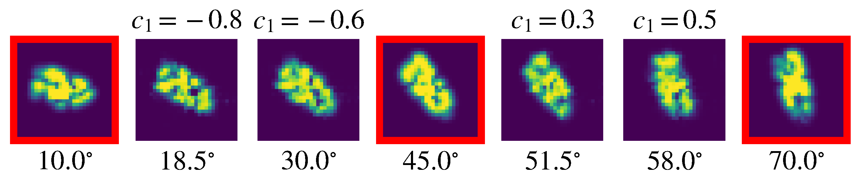
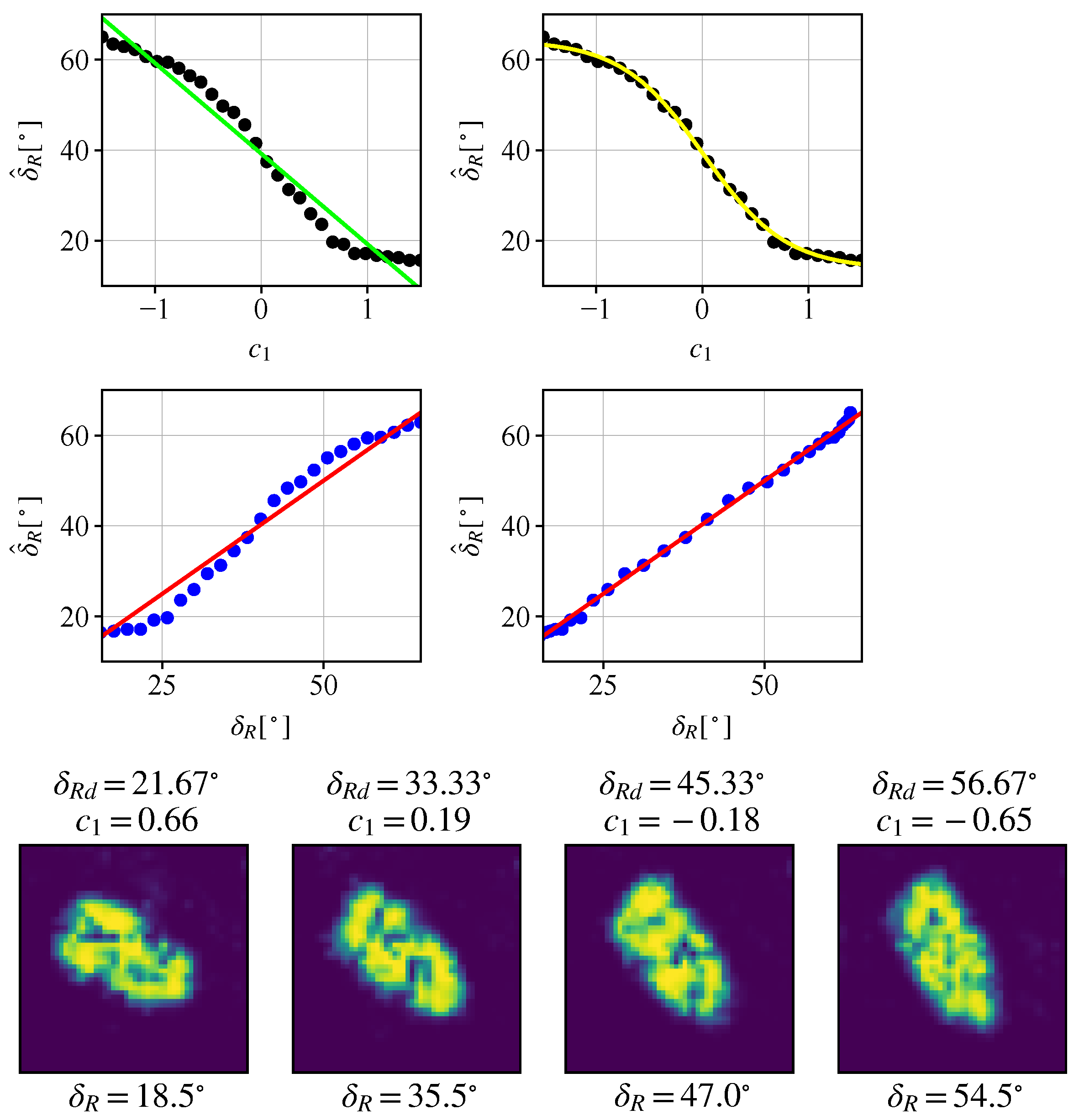
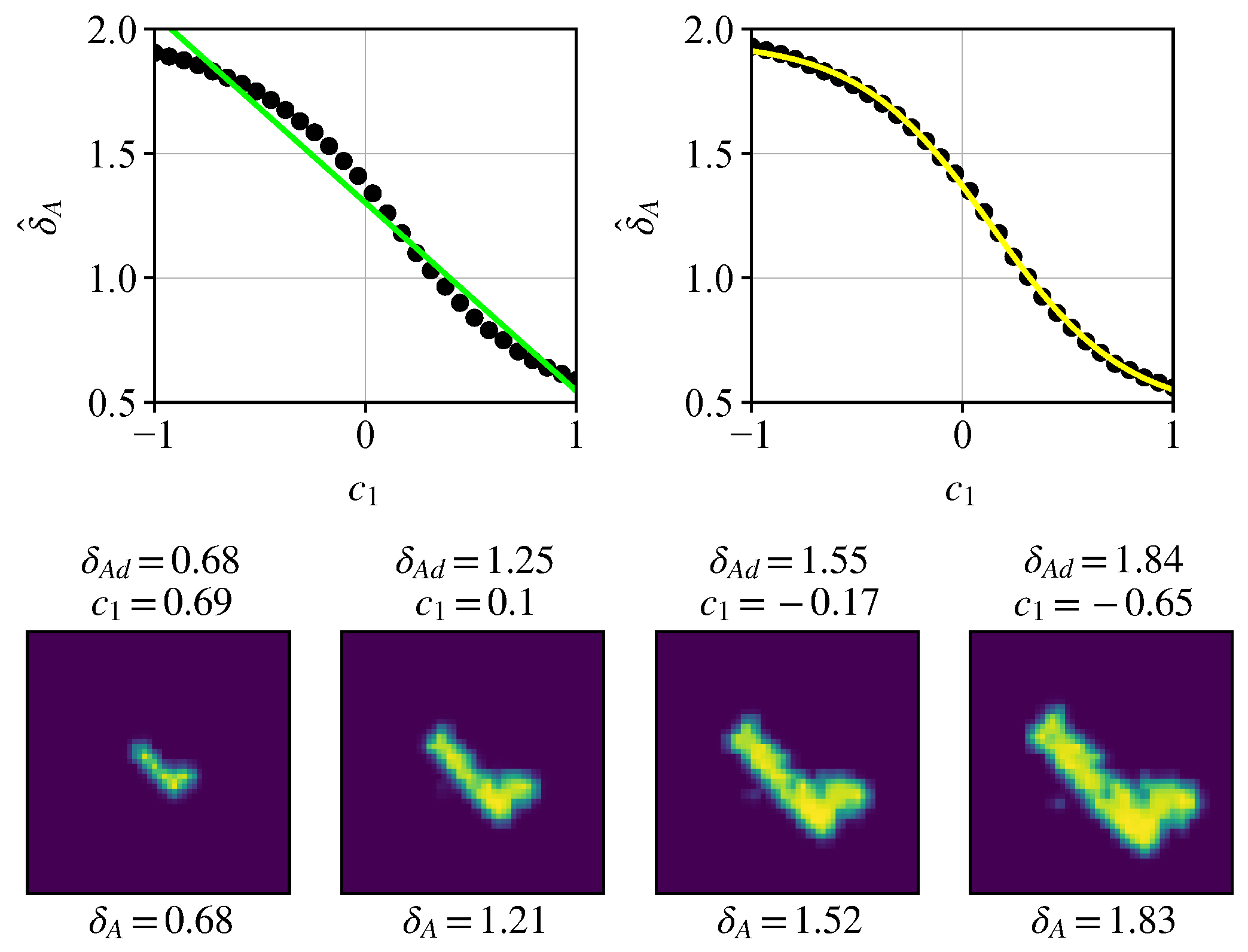
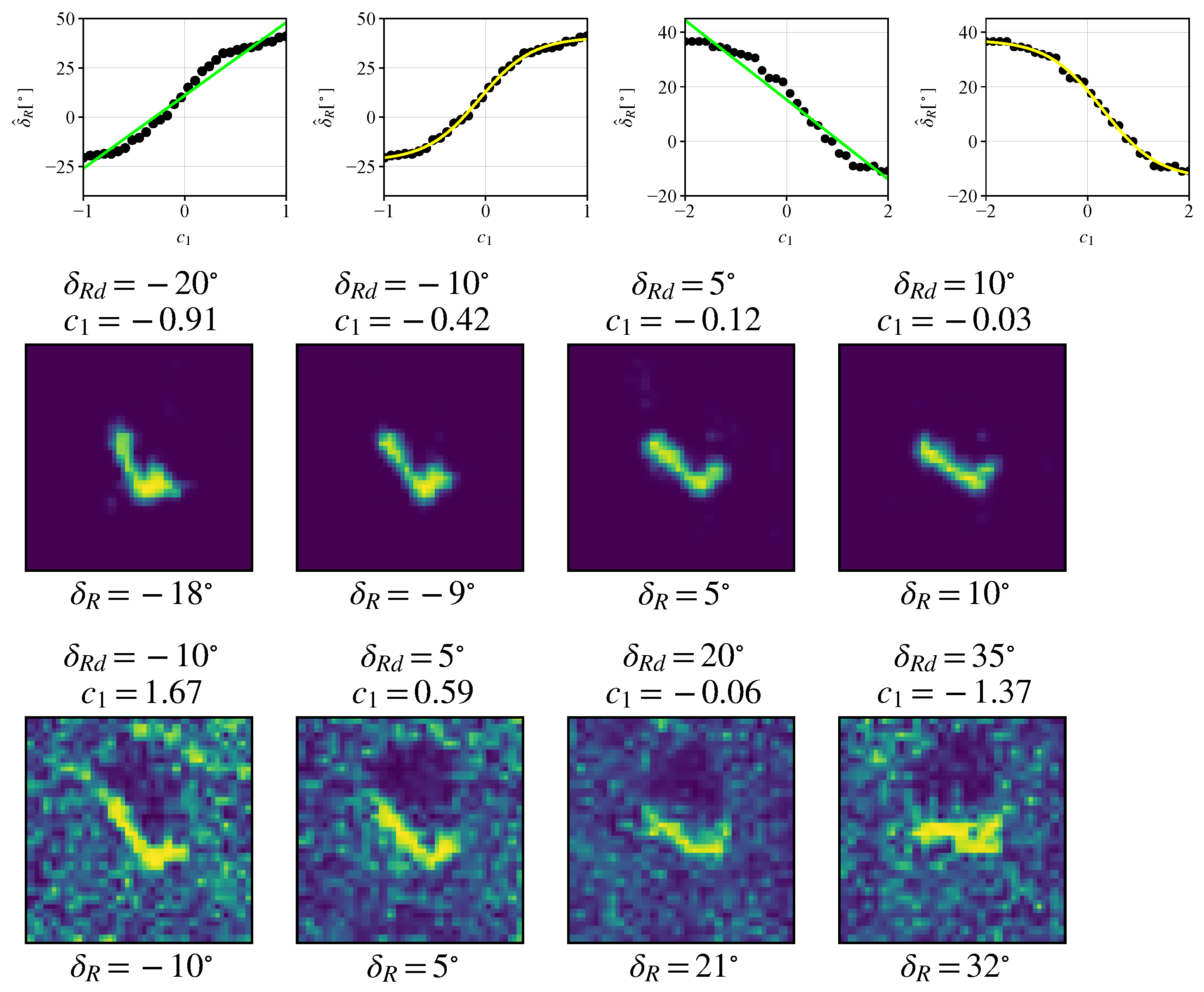
4.2.1. One Property—One Latent Code

All three properties were considered separately: for rotation, a real SAR image was analytically rotated from $-30$ to 30 degrees to obtain 601 images; for translation, the target in a real image was translated from $-6$ to 6 pixels from the original position to obtain 151 images; for scaling, the target in a real image was scaled from $0.5$ to 2 times of the original size to obtain 301 images. After the InfoGAN was trained independently with three datasets, respectively (in three separate experiments), we synthesized the new images corresponding to the various values of the latent code, $c_1\left(1\right),\cdots ,c_1\left(K\right),K=30$, uniformly sampled from the interval $[-1.0,1.0]$ for each property. Then, the properties, ${\delta }_R$, ${\delta }_S$, and ${\delta }_A$ can be measured by (19) and the estimated properties, ${\widehat{\delta }}_R$, ${\widehat{\delta }}_S$, and ${\widehat{\delta }}_A$, can be calculated using (20) and (25). The comparison of the measured properties and estimated properties shows that the nonlinear estimator performs better than the linear estimator in all cases, especially for rotation (top-right) and scaling (bottom-right), as shown in Figure 8. For each case, we synthesized SAR images for four desired ${\delta }_{Rd}$, ${\delta }_{Sd}$, and ${\delta }_{Ad}$, respectively, using $c_1$ calculated by (26). The estimated properties of the synthesized SAR images, ${\delta }_R$, ${\delta }_S$, and ${\delta }_A$, are measured by (19). We can see that the agreement is good in all considered cases.

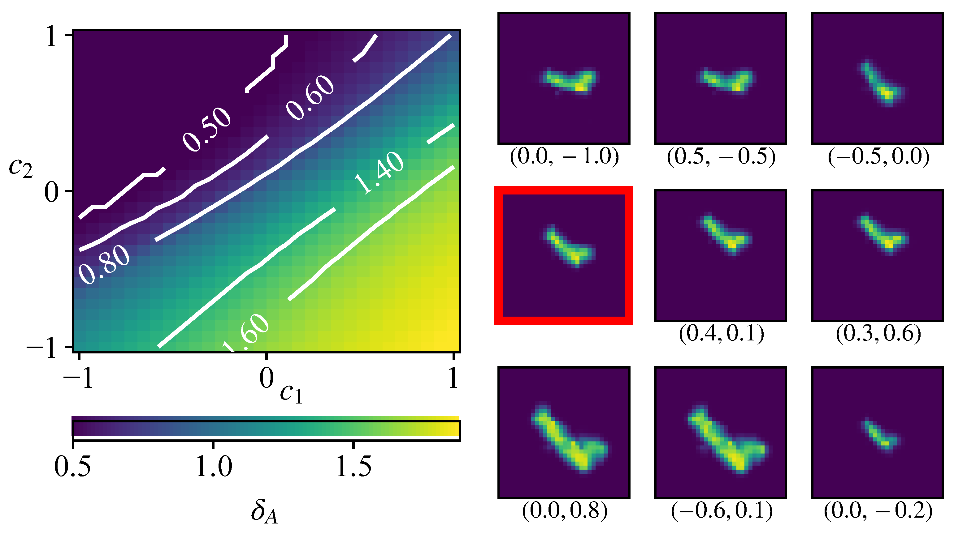
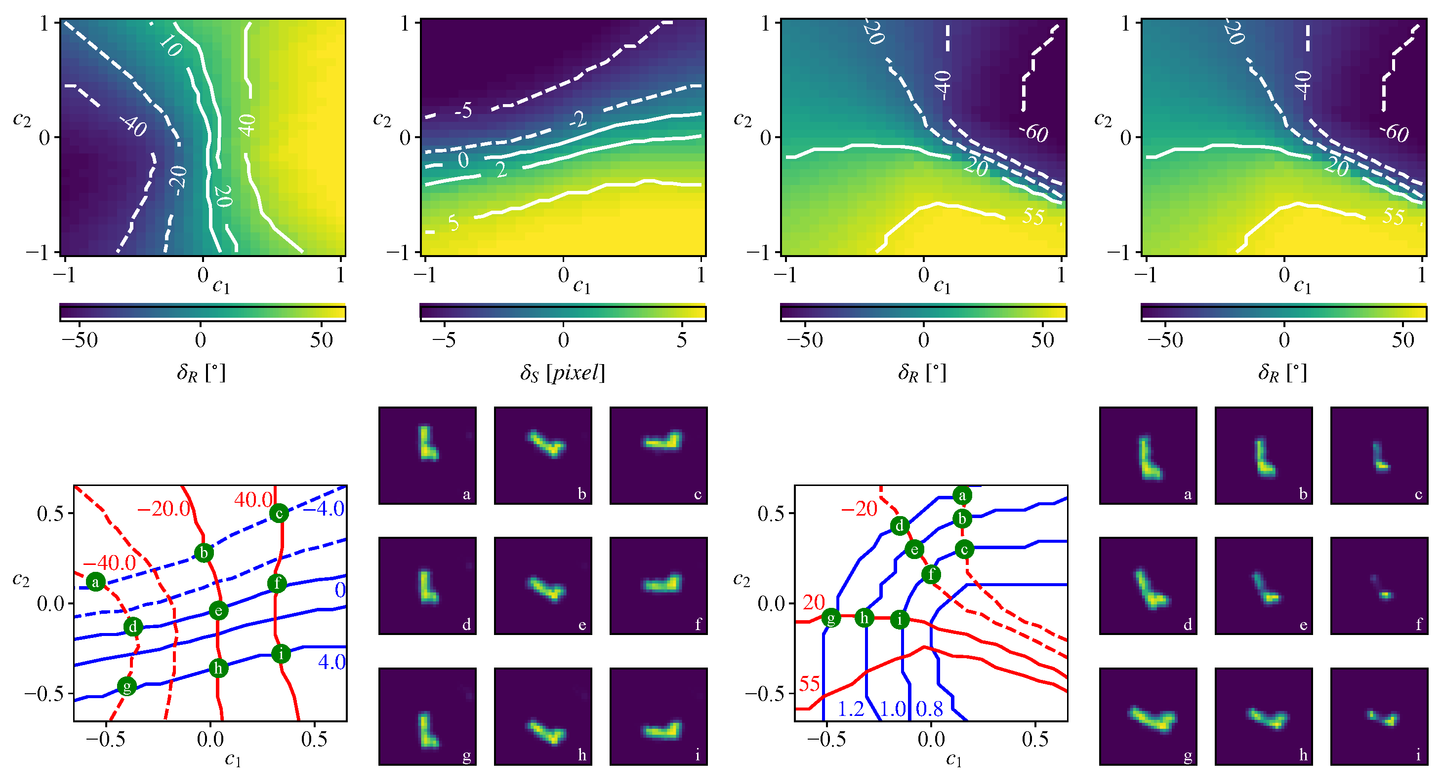
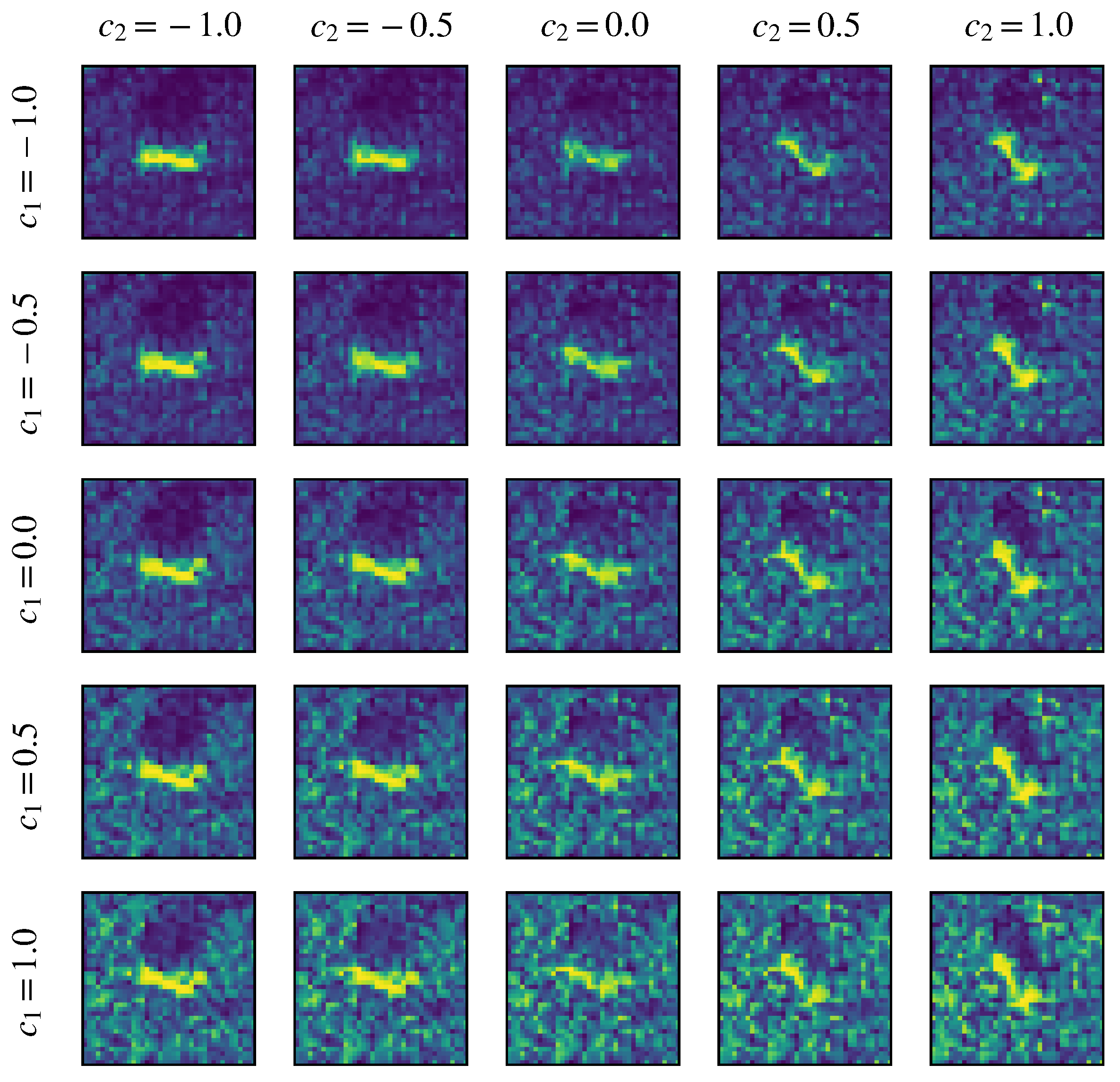
4.2.2. One Property—Two Latent Codes

Now, we introduce two latent codes $c_1$ and $c_2$ to train the InfoGAN with input images exhibiting one-property variations in order to check whether one property will remain within one latent code or will propagate to the other latent code as well. We use completely the same data as in Section 4.2.1, i.e., the only difference is that two latent codes are considered here. Taking rotation, for instance, we have generated 900 images with ${\delta }_R(k_1,k_2)$, $k_1,k_2=1,2,\cdots ,30$, from the InfoGAN trained with both $c_1$ and $c_2$ activated. Figure 9 reveals that the value of a specific property is spread over the available latent codes and therefore is determined by multiple pairs of $c_1$ and $c_2$, because the solution to (31) is not unique, as discussed in Section 3.

To show this relation vividly, we generated several SAR images by using some selected values of $c_1$ and $c_2$, as shown in Figure 9 (bottom-right). In this panel, consisting of $3\times 3$ images, the first and the second image in the top row are with different $c_1$ and $c_2$ but both result in the same ${\delta }_R=-{20}^{\circ }$. In comparison, the third one in the top row shows ${\delta }_R={25}^{\circ }$ with $c_1=-0.5$ and $c_2=0.0$. This comparison further demonstrates the solution to (27) is not unique. This conclusion is also applicable to ${\delta }_S$ and ${\delta }_A$ as shown in the second and the third row; thus, it is feasible to retain or change any property by manipulating $c_1$ and $c_2$. Finally, the properties measured by (19) and the estimated properties using (30) are compared in Figure 10 to validate the performance of the estimator (only the nonlinear model is considered because the relation between one property and two latent codes is obviously much more complex than the linear model). The results show that ${\widehat{\delta }}_R$, ${\widehat{\delta }}_S$, and ${\widehat{\delta }}_A$, calculated by (30), basically match the ${\delta }_R$, ${\delta }_S$, and ${\delta }_A$, respectively, even though the accuracy is slightly lower than in Figure 9.

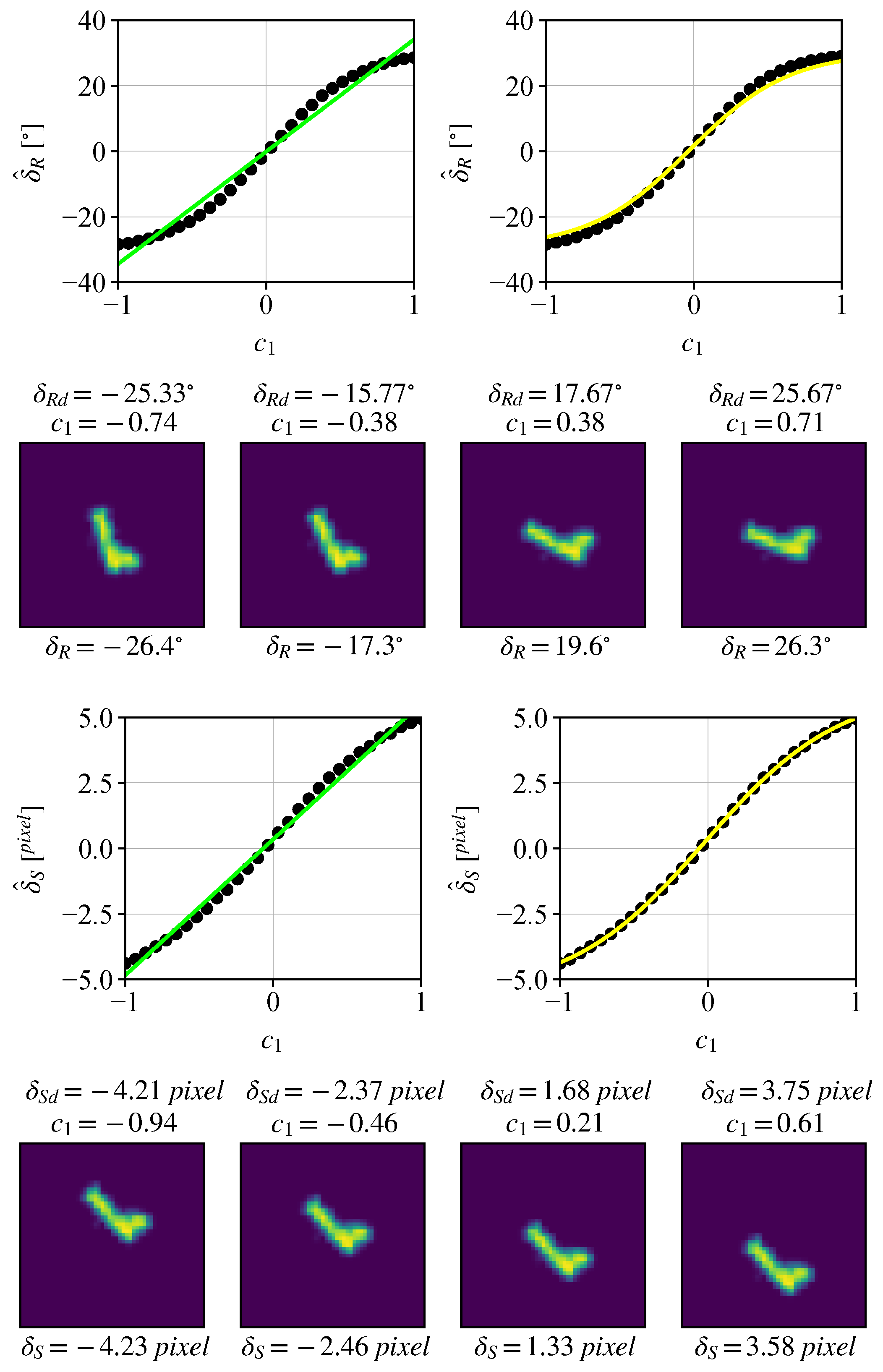
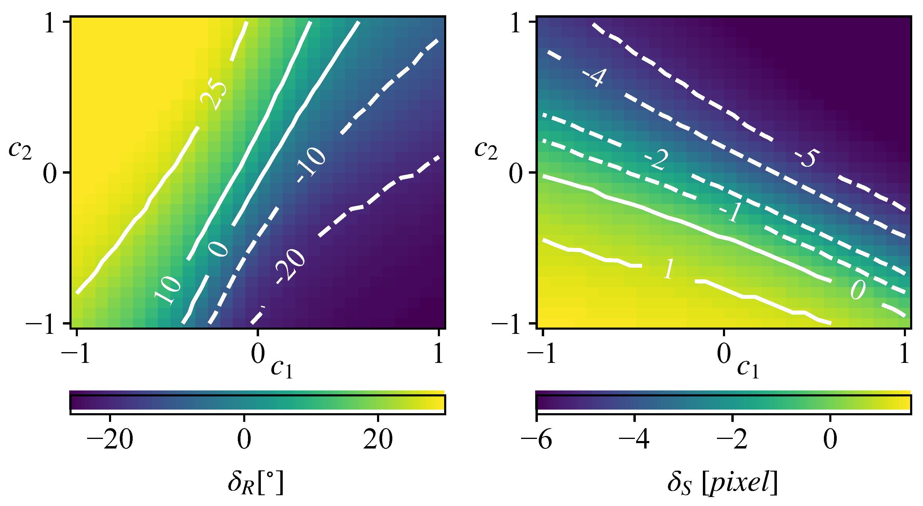
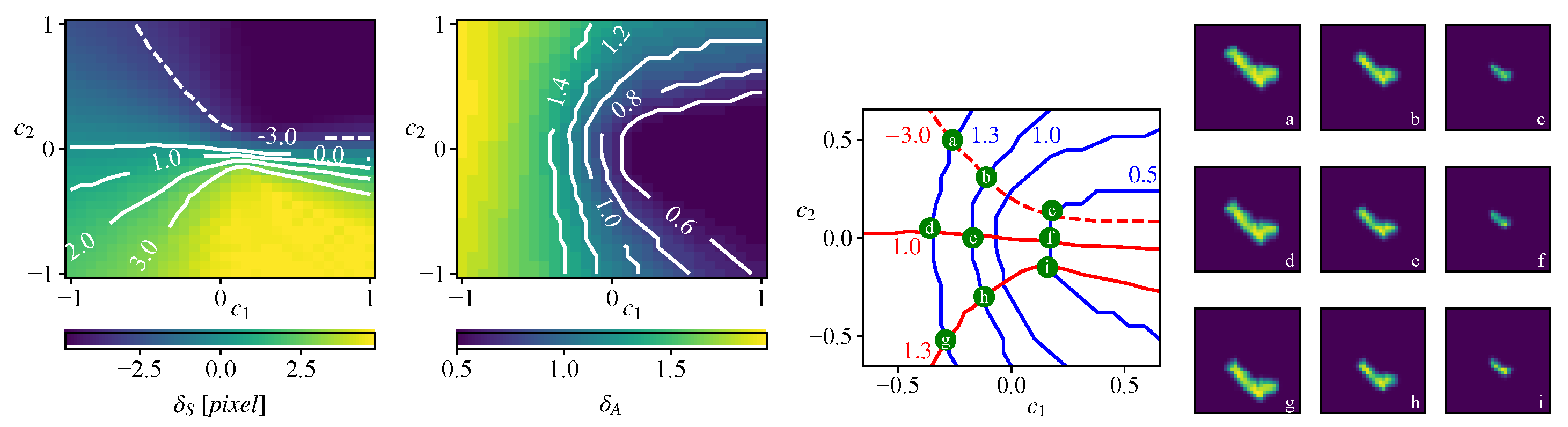
4.2.3. Two Properties—Two Latent Codes

In this experiment, we consider two entangled properties emerging in each training SAR image simultaneously. Firstly, we generate three combinations of training data: rotation–translation, rotation–scaling, and translation–scaling. For rotation–translation, there are 3721 training images with 61 rotation angles uniformly dividing $[-{60}^{\circ },{60}^{\circ }]$ and 61 translation pixels uniformly dividing $[-6,6]$. For rotation–scaling, there are 1891 training images with 31 scaling uniformly dividing $[0.5,2]$ and 61 rotation angles uniformly dividing $[-{60}^{\circ },{60}^{\circ }]$. For translation–scaling, there are 3751 training images with 121 translation pixels uniformly dividing $[-6,6]$ and 31 scaling uniformly dividing $[0.5,2]$. We have generated 900 images for each property using different combinations of $c_1$ and $c_2$ and show their relation in Figure 11 and Figure 12. Next, we conduct an experiment to visualize how to edit the entangled properties by manipulating $c_1$ and $c_2$. In each case, we select 9 combinations of $c_1$ and $c_2$ in intersections of two contour lines (green dots in the bottom-left of Figure 11 and Figure 12). The synthesized SAR images, by using these ($c_1$, $c_2$) in the bottom-right, show that if $c_1$ and $c_2$ are along one curve only the property corresponding to this curve will be changed while the other property remains still. Furthermore, given two desired properties, for example, ${\delta }_{Rd}$ and ${\delta }_{Sd}$, the satisfying combination of $c_1$ and $c_2$ is unique in a certain range (the green dots). Thus, it is feasible to precisely edit either a single property or two properties simultaneously by manipulating $c_1$ and $c_2$ as we expected.

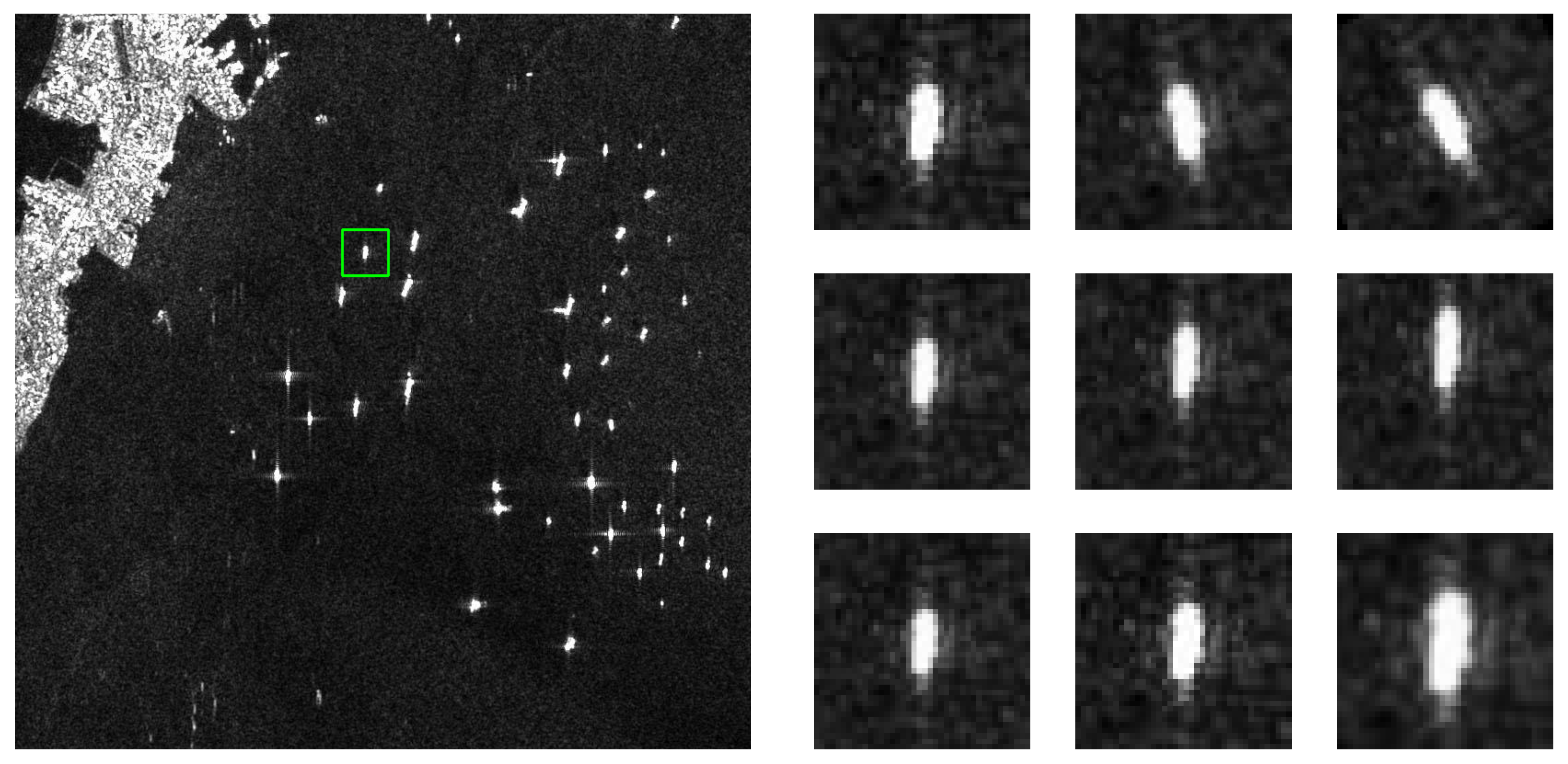
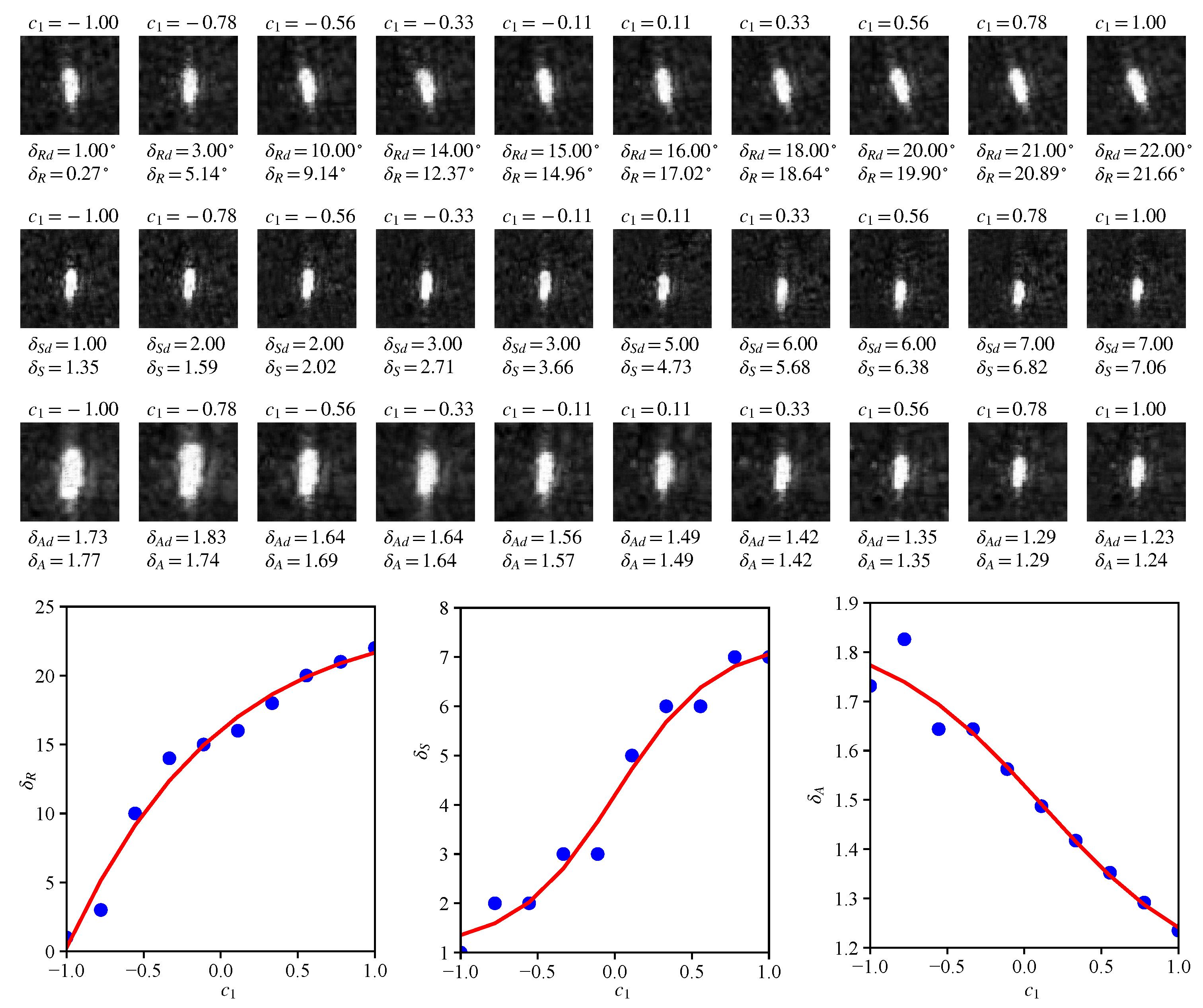
4.3. Real SAR Images with Suppressed Background

The real-measured dataset is a MSTAR dataset with SAR images of ground stationary targets released by the MSTAR program supported by the Defense Advanced Research Projects Agency (DARPA) of the United States [42]. The MSTAR dataset includes 2536 SAR images for training and 2636 for testing with 10 classes of vehicles. We chose 60 images of 2S1 (self-propelled artillery) with rotation angles (with respect to one called the reference SAR image) from $[-{34}^{\circ }$, ${44}^{\circ }]$. The images are downsampled to the size of $28\times 28$ pixels.

After the InfoGAN was trained with only $c_1$ activated, the same experiments as for simulated SAR images were conducted, as shown in Figure 13. We can see that the latent code $c_1$, after the training process, is associated with the SAR image rotation. The modeling of the rotation angle and the latent code was performed using the linear and nonlinear model (Figure 13, top row). While the linear model is simple, the nonlinear model fits the data better. Finally, the model was used to synthesize new SAR images for a given desired rotation angle, ${\delta }_{Rd}$. The obtained images are shown in the bottom row of Figure 13 for four desired angles. The estimated rotation angles, ${\widehat{\delta }}_R$, of the SAR images synthesized with $c_1$ calculated by (26), are given in this panel as well, and we can see that they are close to the desired ones, ${\delta }_{Rd}$.

4.4. SAR Images with Background

Furthermore, we conducted the same experiments with real SAR images, but not removing the background, and the results are similar to the previous experiment, as shown in Figure 13, where the measured and modeled rotation angle is shown (with respect to the reference SAR image). Four synthesized SAR images with the desired rotation, controlled by the latent code values, are given in Figure 13 (bottom). The experiment with the included background was repeated with two latent codes in the InfoGAN. Some synthesized SAR images are shown in Figure 14. As can be seen from this figure, the latent code $c_1$ controls the rotation, while the latent code $c_2$, in this case, takes control over the background intensity. Thus, if we want to obtain images with suppressed backgrounds, we can use high values of $c_2$.

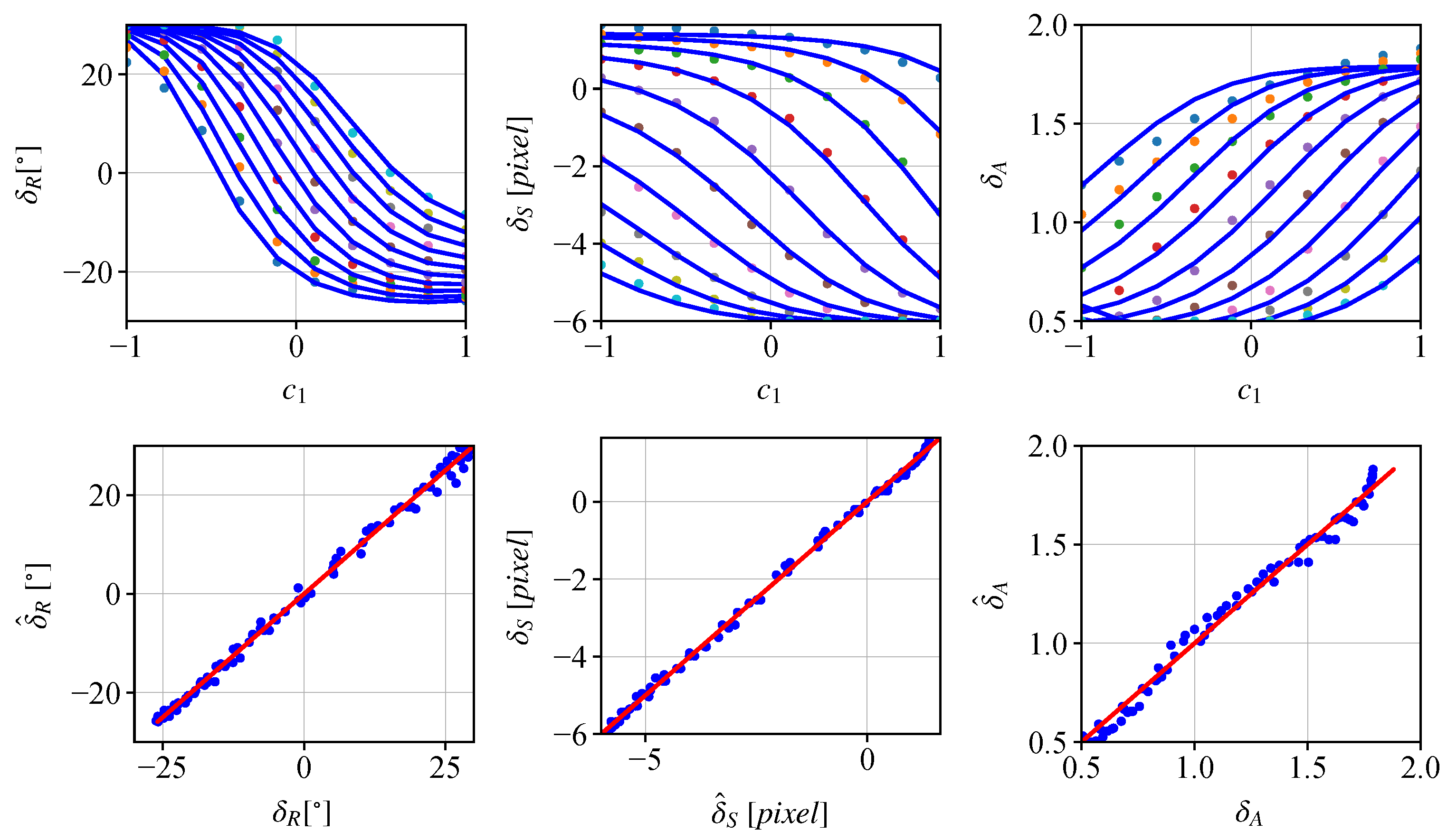
4.5. Robustness and Generalization Analysis on Other SAR Datasets

Here, we introduce another dataset, AIR-SARShip-1.0 (released by the Chinese Academy of Sciences and University of Chinese Academy of Sciences), to further demonstrate the robustness and generalization of the proposed method. AIR-SARShip-1.0 comprises 31 images from Gaofen-3 satellite SAR images, including harbors, islands, reefs, and the sea surface in different conditions. The backgrounds include various scenarios, such as the nearshore and open sea. We selected a SAR image indexed as 05_8_21 from the AIR-SARShip-1.0 and cropped a slice of a ship target as a baseline image, shown in Figure 15. Then we manually imposed three properties to the baseline image, as in Section 4. Specifically, there are 30 images uniformly dividing the rotation range (from $1^{\circ }$ to ${30}^{\circ }$), 15 images uniformly dividing the translation range (from 1 to 15 pixels), and 15 images uniformly dividing the scaling range (from 1 to $1.8$), as shown in Figure 15.

Next, we implemented the same experiments on these three groups of SAR images to interpret the relation between each property and the latent code, $c_1$. Figure 16 presents the synthesized SAR images and estimated values of the properties. A similar conclusion can be drawn to the previous experiments, which further proves the robustness and generalization of our method on different datasets.

5. Discussion

The experiments were carried out with four datasets: simulated images, real objects from SAR images with simulated properties, SAR images with suppressed backgrounds, and SAR images with backgrounds. In the first experimental setup, the results demonstrate that the relation between a single latent code and one property matches a sigmoid function. In the second case, the results show that quadratic terms in the argument are required to cater to more complex relations when two latent codes are considered. The third and fourth experimental setups further demonstrate such a conclusion is applicable to real SAR images. Therefore, it is possible to synthesize SAR images of these properties by manipulating latent codes according to such a relation interpreted by our proposed method.

6. Conclusions

This paper sheds some light on interpreting the relation between different properties of SAR images and latent codes in the InfoGAN. In general, the unclear relation between properties and latent codes is modeled in a numerical manner by proposing property estimators. Specifically, the trend of how properties vary with latent codes can be measured mathematically, i.e., the corresponding property can be computed regarding a specific collocation of latent codes and the latent codes can also be computed provided some desired properties. In this case, it is feasible to produce a large scale of photo-realistic SAR images with numerical properties by manipulating the latent codes in the InfoGAN, which could alleviate the shortage of data for deep learning techniques with SAR images.

References

1. Ender, J.; Amin, M.G.; Fornaro, G.; Rosen, P.A. Recent Advances in Radar Imaging. IEEE Signal Process. Mag. 2014, 31, 15. [Google Scholar] [CrossRef]
2. Moreira, A.; Prats-Iraola, P.; Younis, M.; Krieger, G.; Hajnsek, I.; Papathanassiou, K.P. A Tutorial on Synthetic Aperture Radar. IEEE Geosci. Remote Sens. Mag. 2013, 1, 6–43. [Google Scholar] [CrossRef] [Green Version]
3. Song, L.; Bai, B.; Li, X.; Niu, G.; Liu, Y.; Zhao, L. Space-Time Varying Plasma Sheath Effect on Hypersonic Vehicle-borne SAR Imaging. IEEE Trans. Aerosp. Electron. Syst. 2022, 58, 4527–4539. [Google Scholar] [CrossRef]
4. Ge, B.; An, D.; Chen, L.; Wang, W.; Feng, D.; Zhou, Z. Ground Moving Target Detection and Trajectory Reconstruction Methods for Multi-Channel Airborne Circular SAR. IEEE Trans. Aerosp. Electron. Syst. 2022, 58, 2900–2915. [Google Scholar] [CrossRef]
5. Berizzi, F.; Martorella, M.; Giusti, E. Radar Imaging for Maritime Observation; CRC Press: Boca Raton, FL, USA, 2018. [Google Scholar]
6. Popović, V.; Djurović, I.; Stanković, L.; Thayaparan, T.; Daković, M. Autofocusing of SAR Images Based on Parameters Estimated from the PHAF. Signal Process. 2010, 90, 1382–1391. [Google Scholar] [CrossRef]
7. Franceschetti, G.; Guida, R.; Iodice, A.; Riccio, D.; Ruello, G. Efficient Simulation of Hybrid Stripmap/Spotlight SAR Raw Signals from Extended Scenes. IEEE Trans. Geosci. Remote Sens. 2004, 42, 2385–2396. [Google Scholar] [CrossRef]
8. Ding, B.; Wen, G.; Huang, X.; Ma, C.; Yang, X. Data Augmentation by Multilevel Reconstruction Using Attributed Scattering Center for SAR Target Recognition. IEEE Geosci. Remote Sens. Lett. 2017, 14, 979–983. [Google Scholar] [CrossRef]
9. Diederik, P.; Kingma, M.W. Auto-Encoding Variational Bayes. arXiv 2013, arXiv:1312.6114. [Google Scholar]
10. Qian, D.; Cheung, W.K. Learning Hierarchical Variational Autoencoders With Mutual Information Maximization for Autoregressive Sequence Modeling. IEEE Trans. Pattern Anal. Mach. Intell. 2023, 45, 1949–1962. [Google Scholar] [CrossRef]
11. Jin, F.; Sengupta, A.; Cao, S. mmFall: Fall Detection Using 4-D mmWave Radar and a Hybrid Variational RNN AutoEncoder. IEEE Trans. Autom. Sci. Eng. 2022, 19, 1245–1257. [Google Scholar] [CrossRef]
12. Goodfellow, I.; Pouget-Abadie, J.; Mirza, M.; Xu, B.; Warde-Farley, D.; Ozair, S.; Courville, A.; Bengio, Y. Generative Adversarial Nets. Adv. Neural Inf. Process. Syst. 2014, 63, 139–144. [Google Scholar]
13. Doi, K.; Sakurada, K.; Onishi, M.; Iwasaki, A. GAN-Based SAR-to-Optical Image Translation with Region Information. In Proceedings of the IGARSS 2020—2020 IEEE International Geoscience and Remote Sensing Symposium, Waikoloa, HI, USA, 26 September–2 October 2020; pp. 2069–2072. [Google Scholar]
14. Du, S.; Hong, J.; Wang, Y.; Qi, Y. A High-Quality Multicategory SAR Images Generation Method With Multiconstraint GAN for ATR. IEEE Geosci. Remote Sens. Lett. 2022, 19, 1–5. [Google Scholar] [CrossRef]
15. Liu, Q.; Zhou, H.; Xu, Q.; Liu, X.; Wang, Y. PSGAN: A Generative Adversarial Network for Remote Sensing Image Pan-Sharpening. IEEE Trans. Geosci. Remote Sens. 2021, 59, 10227–10242. [Google Scholar] [CrossRef]
16. Xie, W.; Cui, Y.; Li, Y.; Lei, J.; Du, Q.; Li, J. HPGAN: Hyperspectral Pansharpening Using 3-D Generative Adversarial Networks. IEEE Trans. Geosci. Remote Sens. 2021, 59, 463–477. [Google Scholar] [CrossRef]
17. Nichol, A.; Dhariwal, P.; Ramesh, A.; Shyam, P.; Sishkin, P.; McGrew, B.; Sutskever, I.; Chen, M. GLIDE: Towards Photorealistic Image Generation and Editing with Text-Guided Diffusion Models. arXiv 2021, arXiv:2112.10741v3. [Google Scholar]
18. Ramesh, A.; Dhariwal, P.; Nichol, A.; Chu, C.; Chen, M. Hierarchical Text-Conditional Image Generation with CLIP Latents. arXiv 2022, arXiv:2204.06125. [Google Scholar]
19. Saharia, C.; Chan, W.; Saxena, S.; Li, L.; Whang, J.; Denton, E.; Ghasemipour, S.K.S.; Ayan, B.K.; Madhavi, S.S.; Lopez, R.G.; et al. Photorealistic Text-to-Image Diffusion Models with Deep Language Understanding. arXiv 2022, arXiv:2205.11487. [Google Scholar]
20. Rombach, R.; Blattmann, A.; Lorenz, D.; Esser, P.; Ommer, B. High-resolution image synthesis with latent diffusion models. In Proceedings of the IEEE/CVF Conference on Computer Vision and Pattern Recognition, New Orleans, LA, USA, 19–24 June 2022; pp. 10684–10695. [Google Scholar]
21. Ho, J.; Jain, A.; Abbeel, P. Denoising Diffusion Probabilistic Models. Adv. Neural Inf. Process. Syst. 2020, 33, 6840–6851. [Google Scholar]
22. Pan, Z.; Yu, W.; Yi, X.; Khan, A.; Yuan, F.; Zheng, Y. Recent Progress on Generative Adversarial Networks (GANs): A Survey. IEEE Access 2019, 7, 36322–36333. [Google Scholar] [CrossRef]
23. Yang, C.; Shen, Y.; Zhou, B. Semantic hierarchy emerges in deep generative representations for scene synthesis. Int. J. Comput. Vis. 2021, 129, 1451–1466. [Google Scholar] [CrossRef]
24. Chen, X.; Duan, Y.; Houthooft, R.; Schulman, J.; Sutskever, I.; Abbeel, P. Infogan: Interpretable Representation Learning by Information Maximizing Generative Adversarial Nets. In Proceedings of the 30th Conference on Neural Information Processing Systems (NIPS 2016), Barcelona, Spain, 5–10 December 2016; p. 29. [Google Scholar]
25. Schwegmann, C.P.; Kleynhans, W.; Salmon, B.P.; Mdakane, L.W.; Meyer, R.G. Synthetic Aperture Radar Ship Discrimination, Generation and Latent Variable Extraction using Information Maximizing Generative Adversarial Networks. In Proceedings of the 2017 IEEE International Geoscience and Remote Sensing Symposium (IGARSS), Fort Worth, TX, USA, 23–28 July 2017; IEEE: Piscataway, NJ, USA, 2017; pp. 2263–2266. [Google Scholar]
26. Martorella, M.; Giusti, E.; Demi, L.; Zhou, Z.; Cacciamano, A.; Berizzi, F.; Bates, B. Target Recognition by Means of Polarimetric ISAR Images. IEEE Trans. Aerosp. Electron. Syst. 2011, 47, 225–239. [Google Scholar] [CrossRef]
27. Wu, Q.; Zhang, Y.D.; Amin, M.G.; Himed, B. High-resolution Passive SAR Imaging Exploiting Structured Bayesian Compressive Sensing. IEEE J. Sel. Top. Signal Process. 2015, 9, 1484–1497. [Google Scholar] [CrossRef]
28. Papson, S.; Narayanan, R.M. Classification via the Shadow Region in SAR Imagery. IEEE Trans. Aerosp. Electron. Syst. 2012, 48, 969–980. [Google Scholar] [CrossRef]
29. Stanković, L.; Brajović, M.; Stanković, I.; Ioana, C.; Daković, M. Reconstruction Error in Nonuniformly Sampled Approximately Sparse Signals. IEEE Geosci. Remote Sens. Lett. 2021, 18, 28–32. [Google Scholar] [CrossRef]
30. Stanković, L. ISAR Image Analysis and Recovery with Unavailable or Heavily Corrupted Data. IEEE Trans. Aerosp. Electron. Syst. 2015, 51, 2093–2106. [Google Scholar] [CrossRef] [Green Version]
31. Brisken, S.; Martorella, M.; Mathy, T.; Wasserzier, C.; Worms, J.G.; Ender, J.H. Motion Estimation and Imaging with a Multistatic ISAR System. IEEE Trans. Aerosp. Electron. Syst. 2014, 50, 1701–1714. [Google Scholar] [CrossRef]
32. Arnous, F.I.; Narayanan, R.M.; Li, B.C. Application of Multidomain Data Fusion, Machine Learning and Feature Learning Paradigms Towards Enhanced Image-based SAR Class Vehicle Recognition. In Proceedings of the Radar Sensor Technology XXV, International Society for Optics and Photonics, Online, 12–17 April 2021; Volume 11742, p. 1174209. [Google Scholar]
33. Franceschetti, G.; Schirinzi, G. A SAR Processor Based on Two-dimensional FFT Codes. IEEE Trans. Aerosp. Electron. Syst. 1990, 26, 356–366. [Google Scholar] [CrossRef]
34. Zhang, S.; Pavel, M.S.R.; Zhang, Y.D. Crossterm-free Time-frequency Representation Exploiting Deep Convolutional Neural Network. Signal Process. 2022, 192, 108372. [Google Scholar] [CrossRef]
35. Belloni, C.; Balleri, A.; Aouf, N.; Le Caillec, J.M.; Merlet, T. Explainability of Deep SAR ATR Through Feature Analysis. IEEE Trans. Aerosp. Electron. Syst. 2021, 57, 659–673. [Google Scholar] [CrossRef]
36. Fahimi, F.; Dosen, S.; Ang, K.K.; Mrachacz-Kersting, N.; Guan, C. Generative Adversarial Networks-Based Data Augmentation for Brain–Computer Interface. IEEE Trans. Neural Networks Learn. Syst. 2021, 32, 4039–4051. [Google Scholar] [CrossRef]
37. Song, R.; Huang, Y.; Xu, K.; Ye, X.; Li, C.; Chen, X. Electromagnetic Inverse Scattering With Perceptual Generative Adversarial Networks. IEEE Trans. Comput. Imaging 2021, 7, 689–699. [Google Scholar] [CrossRef]
38. O’Reilly, J.A.; Asadi, F. Pre-trained vs. Random Weights for Calculating Fréchet Inception Distance in Medical Imaging. In Proceedings of the 2021 13th Biomedical Engineering International Conference (BMEiCON), Ayutthaya, Thailand, 19–21 November 2021; pp. 1–4. [Google Scholar]
39. Sekar, A.; Perumal, V. CFC-GAN: Forecasting Road Surface Crack Using Forecasted Crack Generative Adversarial Network. IEEE Trans. Intell. Transp. Syst. 2022, 23, 21378–21391. [Google Scholar] [CrossRef]
40. Chen, S.J.; Shen, H.L. Multispectral Image Out-of-Focus Deblurring Using Interchannel Correlation. IEEE Trans. Image Process. 2015, 24, 4433–4445. [Google Scholar] [CrossRef] [PubMed]
41. Pu, W. SAE-Net: A Deep Neural Network for SAR Autofocus. IEEE Trans. Geosci. Remote Sens. 2022, 60, 1–14. [Google Scholar] [CrossRef]
42. The Sensor Data Management System, MSTAR Database. Available online: https://www.sdms.afrl.af.mil/index.php?collection=mstar (accessed on 3 August 2022).
43. Feng, Z.; Zhu, M.; Stanković, L.; Ji, H. Self-matching CAM: A Novel Accurate Visual Explanation of CNNs for SAR Image Interpretation. Remote Sens. 2021, 13, 1772. [Google Scholar] [CrossRef]
44. Feng, Z.; Ji, H.; Stanković, L.; Fan, J.; Zhu, M. SC-SM CAM: An Efficient Visual Interpretation of CNN for SAR Images Target Recognition. Remote Sens. 2021, 13, 4139. [Google Scholar] [CrossRef]
Figure 1. Synthetic aperture radar setup with various relative positions of the radar and the target. The mechanism of SAR imaging (left). The emergence of scaling of the target in a SAR image (middle). The emergence of rotation and translation of the target in a SAR image (right).
Remotesensing 15 01254 g001
Figure 2. The architecture of GAN and InfoGAN. The basic GAN is obtained by excluding the red blocks and latent codes c .
Remotesensing 15 01254 g002
Figure 3. The comparison of generated SAR images between GAN and InfoGAN. The rotation angles are not controllable in GAN (left). The rotation angles are highly related to the latent code, c 1 (right).
Remotesensing 15 01254 g003
Figure 4. Illustration of SAR image samples from four datasets considered in the experimental setup: simulated SAR images with different viewing angles (top row); a radar image from the MSTAR dataset, with suppressed background, rotated for various angles (second row); SAR images from MSTAR dataset corresponding to different viewing angles of the same target, with suppressed background (third row); SAR images from MSTAR dataset corresponding to different viewing angles with a background (bottom row).
Remotesensing 15 01254 g004
Figure 5. Some images generated by InfoGAN with different numbers of iterations in the training process: 50 iterations (first); 500 iterations (second); 5000 iterations (third); 10,000 iterations (fourth).
Remotesensing 15 01254 g005
Figure 6. Real and synthesized SAR images for various rotation angles. The first, fourth, and seventh images (marked by red squares) are SAR images used for the training of the InfoGAN, while the second, third, fifth, and sixth images are the SAR images synthesized by the InfoGAN with the latent code values c 1 = 0.8 , 0.6 , 0.3 , 0.5 , respectively.
Remotesensing 15 01254 g006
Figure 7. The results for the estimated and modeled rotation angle for the SAR images synthesized by the InfoGAN trained with simulated SAR images. The rotation angles in SAR images as a function of the latent code, c 1 , measured by cross-correlation (black dots) and the estimated values with a linear model (green line) (top-left). The rotation angles in SAR images as a function of the latent code, c 1 , measured by cross-correlation (black dots) and the estimated values with a nonlinear model (yellow line) (top-right). Comparison of the measured angle values by cross-correlation with the ones obtained using the linear model (blue dots), where the red line denotes the ideal case that δ ^ R ( k ) = δ R ( k ) for all k (middle-left). Comparison of the estimated angle values with the ones obtained using the nonlinear model (blue dots) (middle-right). The synthesized SAR images using c 1 calculated by (26) for four desired rotation angles, δ R d = 21 . 67 , 33 . 33 , 45 . 33 , 56 . 67 (bottom row). The estimated rotations of the synthesized SAR images, δ R ( k ) are calculated using (19). They are close to the desired ones.
Remotesensing 15 01254 g007
Figure 8. The results for the measured and modeled rotation (top), translation (middle), and scaling (bottom) for the SAR images synthesized by the InfoGAN trained with the second dataset. In each case, we show the relation between c 1 and the considered property (dots), approximations using linear (green line in left subplots) and nonlinear models (yellow line in right subplots), and synthesized SAR images using c 1 calculated by (26) for four desired δ R d , δ S d , and δ A d . The estimated properties of the synthesized SAR images, δ R , δ S , and δ A , are measured by (19). They are close to the desired ones.
Remotesensing 15 01254 g008aRemotesensing 15 01254 g008b
Figure 9. The relation between each property and two latent codes. The relation between rotation angle δ R and c 1 , c 2 (top-left). The relation between translation pixels δ S and c 1 , c 2 (top-right). The relation between scaling δ A and c 1 , c 2 (bottom-left). The synthesized SAR images corresponding to ( c 1 , c 2 ) labeled below each image except for the original image (marked by red square) (bottom-right). In this panel (bottom-right), the first two images in the top row exhibit the same rotation angle δ R with different c 1 and c 2 , i.e., c 1 = 0.0 , c 2 = 1.0 and c 1 = 0.5 , c 2 = 0.5 , both resulting in 20 rotation. The third one in the top row shows δ R = 25 with c 1 = 0.5 and c 2 = 0.0 . These figures further demonstrate the solution to (31) is not unique; thus, it is possible to retain or change property by manipulating c 1 and c 2 . This conclusion is also applicable to translation δ S and scaling δ A , as shown in the second and the third rows (bottom-right).
Remotesensing 15 01254 g009aRemotesensing 15 01254 g009b
Figure 10. The comparison of three estimated properties δ ^ R , δ ^ S , and δ ^ A , using (30), and the measured ones, δ R , δ S , and δ A , using (19). The relation with δ R (dots) and two latent codes, c 1 and c 2 (different colors denote different values of c 2 ) (top-left). The δ ^ R is shown with blue lines. They are close to the δ R . The comparison of δ R and δ ^ R (top-right). The results of δ S and δ ^ S are shown in the middle-right and middle-left images, respectively. The results of δ A and δ ^ A are shown in the bottom-right and bottom-left images, respectively.
Remotesensing 15 01254 g010
Figure 11. The relation between rotation–translation and two latent codes. The relation between rotation angle δ R and c 1 , c 2 (top-left). The relation between translation δ S and c 1 , c 2 (top-right). The overlapped curves of the above two contours as well as some selected intersections (green dots) (bottom-left). The synthesized SAR images with ( c 1 , c 2 ) corresponding to the coordinates of the green dots in the former contour (bottom-right). Here nine collocations of c 1 and c 2 are selected and labeled as a, b, c, d, e, f, g, h, and i in contour maps.
Remotesensing 15 01254 g011
Figure 12. The relation between translation–scaling and two latent codes. The relation between translation angle δ S and c 1 , c 2 (top-left). The relation between scaling δ A and c 1 , c 2 (top-right). The overlapped curves of the above two contours as well as some selected intersections (green dots) (bottom-left). The synthesized SAR images with ( c 1 , c 2 ) corresponding to the coordinates of the green dots in the former contour (bottom-right).
Remotesensing 15 01254 g012
Figure 13. The results for the estimated and modeled rotation angle for the SAR images synthesized by the InfoGAN trained with real SAR images. The rotation angles in SAR images as a function of the latent code, c 1 , measured by cross-correlation (black dots) and the estimated values with a linear model (green line) (top-left). The rotation angles in SAR images as a function of the latent code, c 1 , measured by cross-correlation (black dots) and the estimated values with a nonlinear model (yellow line) (top-right). The synthesized SAR images using c 1 calculated by (26) for four desired rotation angles, δ R d = 20 , 10 , 5 , 10 (bottom row). The estimated rotations of the synthesized SAR images, δ R ( k ) , are calculated using (19).
Remotesensing 15 01254 g013
Figure 14. The synthesized SAR images (with background). Two latent codes are used.
Remotesensing 15 01254 g014
Figure 15. Some samples from AIR-SARShip-1.0 dataset. A large-scale SAR image indexed as 05_8_21 in AIR-SARShip-1.0 (left). A slice of one ship (marked by a green box in left subfigure) with three properties manually manipulated (right).
Remotesensing 15 01254 g015
Figure 16. Some experimental results of AIR-SARShip-1.0 dataset. The first, second, and third rows are SAR images produced by InfoGAN with one latent code, c 1 [ 1 , 1 ] , corresponding to rotation, translation, and scaling, respectively. The fourth row shows the comparison between measured rotation (left), translation (middle), and scaling (right) by blue dots and corresponding estimated properties (red curve).
Remotesensing 15 01254 g016