Article

Mapping Forage Biomass and Quality of the Inner Mongolia Grasslands by Combining Field Measurements and Sentinel-2 Observations

1
State Key Laboratory of Vegetation and Environmental Change, Institute of Botany, Chinese Academy of Sciences, Beijing 100093, China
2
University of Chinese Academy of Sciences, Beijing 100049, China
3
Institute of Ecology, College of Urban and Environmental Sciences, and Key Laboratory for Earth Surface Processes of the Ministry of Education, Peking University, Beijing 100871, China
*
Author to whom correspondence should be addressed.
Remote Sens. 2023, 15(8), 1973; https://doi.org/10.3390/rs15081973
Submission received: 20 February 2023 / Revised: 30 March 2023 / Accepted: 3 April 2023 / Published: 8 April 2023

Abstract

:
Grasslands provide essential forage sources for global livestock production. Remote sensing approaches have been widely used to estimate the biomass production of grasslands from regional to global scales, but simultaneously mapping the forage biomass and quality metrics (e.g., crude fiber and crude protein) is still relatively lacking despite an increasing need for better livestock management. We conducted novel gradient grass-cutting experiments and measured hyperspectral reflectance, forage biomass, crude fiber per area (CFarea), and crude protein per area (CParea) across 19 temperate grassland sites in the Xilingol region, Inner Mongolia, China. Based on these measurements, we identified sensitive spectral bands, calculated nine potential spectral indices (Normalized Difference Vegetation Index, Enhanced Vegetation Index, Red Edge Normalized Difference Vegetation Index, Red-Edge Inflection Point, Inverted Red-Edge Chlorophyll Index algorithm, Normalized Difference Red Edge Index, Nitrogen Reflectance Index, Normalized Greenness Index, Land Surface Water Index) and established Random Forest (RF) models that well predicted forage biomass (R2 = 0.67, NRMSE = 12%), CFarea (R2 = 0.59, NRMSE = 14%), and CParea (R2 = 0.77, NRMSE = 10%). Among these nine indices, Land Surface Water Index (LSWI, calculated by R785-900 and R2100-2280) was identified to be the most important predictor and was then used to establish empirical power law models, showing comparable prediction accuracies (forage biomass, R2 = 0.53; NRMSE = 14%; CFarea, R2 = 0.40, NRMSE = 17%; CParea, R2 = 0.72, NRMSE = 11%) in comparison to Random Forest models. Combining the empirical power law models with the LSWI calculated from Sentinel-2 observations, we further mapped the forage biomass and quality and estimated the livestock carrying capacity. The predicted forage biomass, CFarea, and CParea all showed a significant increase with higher mean annual precipitation, but showed no significant correlations with mean annual temperature. Compared with the estimates based on crude protein, the conventional approach solely based on forage biomass consistently overestimated livestock carrying capacity, especially in wetter areas. Our work provides an approach to simultaneously map the forage biomass and quality metrics and recommends a LSWI-based power law model for rapid and low-cost assessment of regional forage status to guide better livestock management.

1. Introduction

Grasslands cover more than one third of the global land area and provide essential forage sources for livestock production and food systems [1,2]. The livestock carrying capacity of grasslands theoretically depends on both forage biomass production and its quality (e.g., contents of crude fiber and crude protein) [3]. Accurately and timely mapping forage biomass and integrated quality metrics on a landscape scale is increasingly needed for better livestock management, especially in grasslands that are sensitive to climate variability and human activities [4,5]. Vegetation indices derived from broadband satellite images, such as the Normalized Difference Vegetation Index (NDVI) and Enhanced Vegetation Index (EVI), have been conventionally used to estimate vegetation biomass and productivity from regional to global scales [6,7,8,9], but these indices perform poorly in estimating forage quality [10]. However, easy-to-use approaches for simultaneous and timely estimates of forage biomass and quality are relatively lacking.
Ground-based, airborne, and/or satellite spectroscopy provide potential tools for rapid and non-destructive estimation of forage quality. Spectral bands in the Visible Near Infrared (VNIR) regions and the Short-Wave Infrared (SWIR) regions have been found to be indicative of leaf Nitrogen (N) due to spectral absorptions by chlorophyll pigments and chlorophyll binding proteins in the VNIR and by other proteins in the SWIR [11,12]. Canopy foliar N content, which is closely related to crude protein (CP), was thus found to show strong positive correlations with canopy spectral reflectance in cultivated grasslands and pastures [13,14]. Crude fiber (CF) content has also been found to show a good relationship with the SWIR spectral bands [15,16] because these bands can reflect the overtones of the chemical groups C-H related to fiber components [17]. However, CF likely shows a weaker correlation with canopy reflection in comparison with CP and biomass [16,18].
The recent development of remote sensing technologies (e.g., UAV hyperspectral imagery) and machine learning algorithms enables more accurate estimation of forage quality [19,20,21]. However, the high cost to acquire hyperspectral data hinders the application-oriented mapping of forage quality and biomass for large areas. Freely available satellite data with fine spatial resolution, such as the Sentinel-2 (S2) multispectral instrument images, provide potential alternative data for evaluating forage quality and biomass in grasslands [16,22,23]. These approaches rely on a labor-intensive and time-consuming field survey across natural gradients in combination with satellite data to establish models for prediction. There is thus a need for alternative approaches to create gradients and establish predictive models. Additionally, compared with the method of machine learning algorithms, single spectral indices are easier to use for rapid and low-cost forage assessment, but such approaches are lacking for simultaneously mapping forage biomass and quality.
Temperate grasslands in the Inner Mongolia Autonomous Region (IMAR) of China are located at the southernmost edge of the Eurasian steppe and provide important ecosystem services, including livestock production [24]. Climate change and overgrazing have resulted in vegetation degradation over the past few decades [25,26]. Consequently, the stability of grassland productivity has decreased significantly and potentially threatens the sustainability of local livestock production systems [27]. In this context, the development of a low-cost and real-time monitoring system for forage biomass and quality is crucial for the conservation and management of regional grassland resources.
In this study, we conducted novel gradient grass-cutting experiments and measured spectral reflectance, forage biomass, crude fiber per area (CFarea), and crude protein per area (CParea) across 19 temperate grassland sites in Xilingol region, IMAR, China. The gradient grass-cutting experiments can facilitate a quick establishment of models to predict regional forage production and quality. Based on the field measurements, we then established Random Forest models and empirical power law models using a single indices to predict forage biomass, CFarea, and CParea. By combining optical remote sensing data (field spectral data and S2 images) with empirical power law models, we further mapped the forage quality and biomass of temperate grasslands in the Xilingol region, IMAR, China. The specific objectives of this study were to: (1) identify the sensitive spectral bands and indices for forage biomass and quality estimation based on gradient grass-cutting experiments, (2) predict forage biomass and quality on the field scale, by establishing spectroscopy-based models (e.g., Random Forest model and empirical regression model), and (3) propose an easy-to-use approach to map the regional forage biomass and quality by combining S2 data with ground-based measurements. Our study estimated CFarea and CParea in a mass per unit area (g/m2, density) because of their important implications for carrying capacity analysis and regional grazing management [12,28].

2. Material and Methods
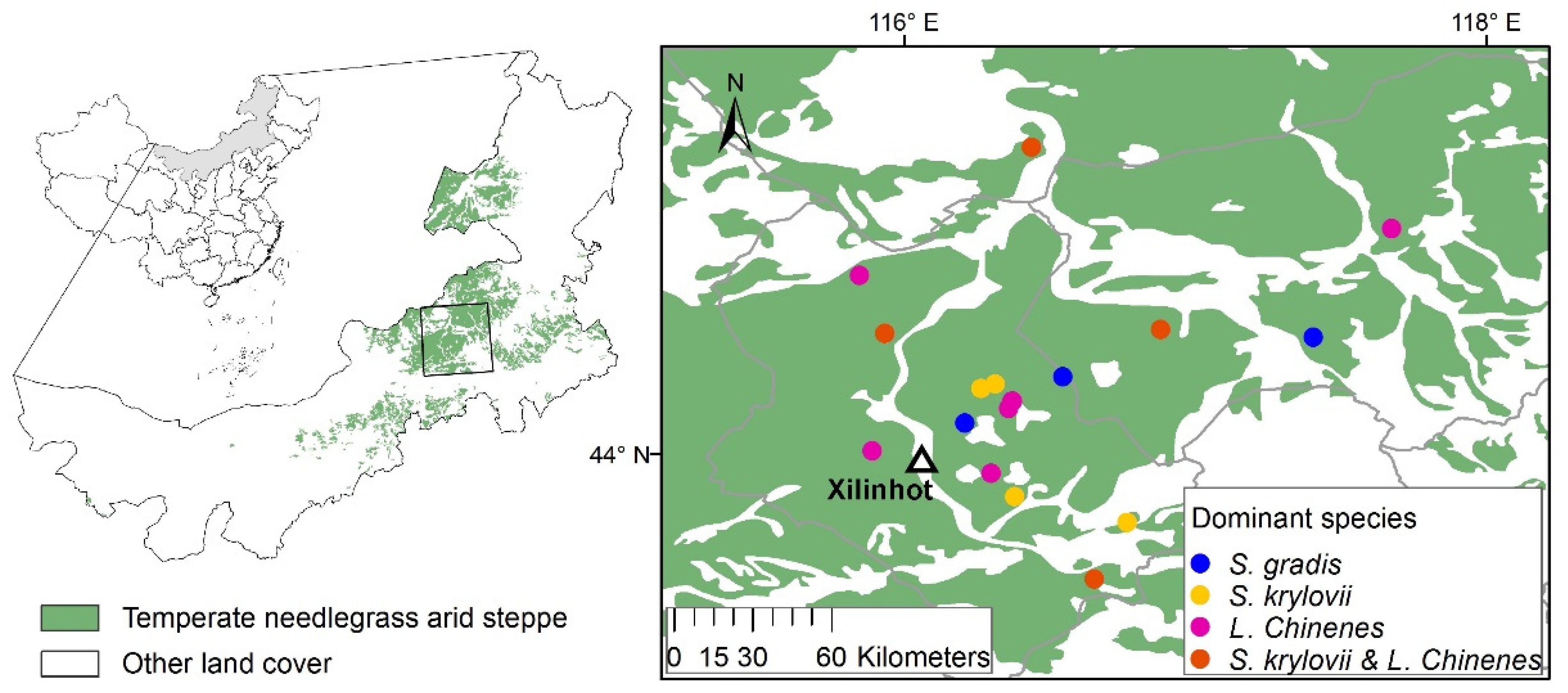
2.1. Study Area

The study was conducted in temperate grasslands in the Xilingol region of IMAR, northern China (Figure 1). This region is characterized by a continental semi-arid climate, with a mean annual precipitation of 267 mm and mean annual temperature of 1.0 °C [27]. Precipitation occurs predominately in summer (June–August) in synchrony with high temperatures. Four types of grassland communities, either dominated by single species such as Leymus chinensis, Stipa grandis, and Stipa Krylovii, or co-dominated by L. chinensis and needlegrass (e.g., S. Krylovii), account for more than 82% of the total vegetation coverage in this region [29]. Three to six replicated sites were randomly selected for each community type, and there were 19 sites in total (Figure 1).

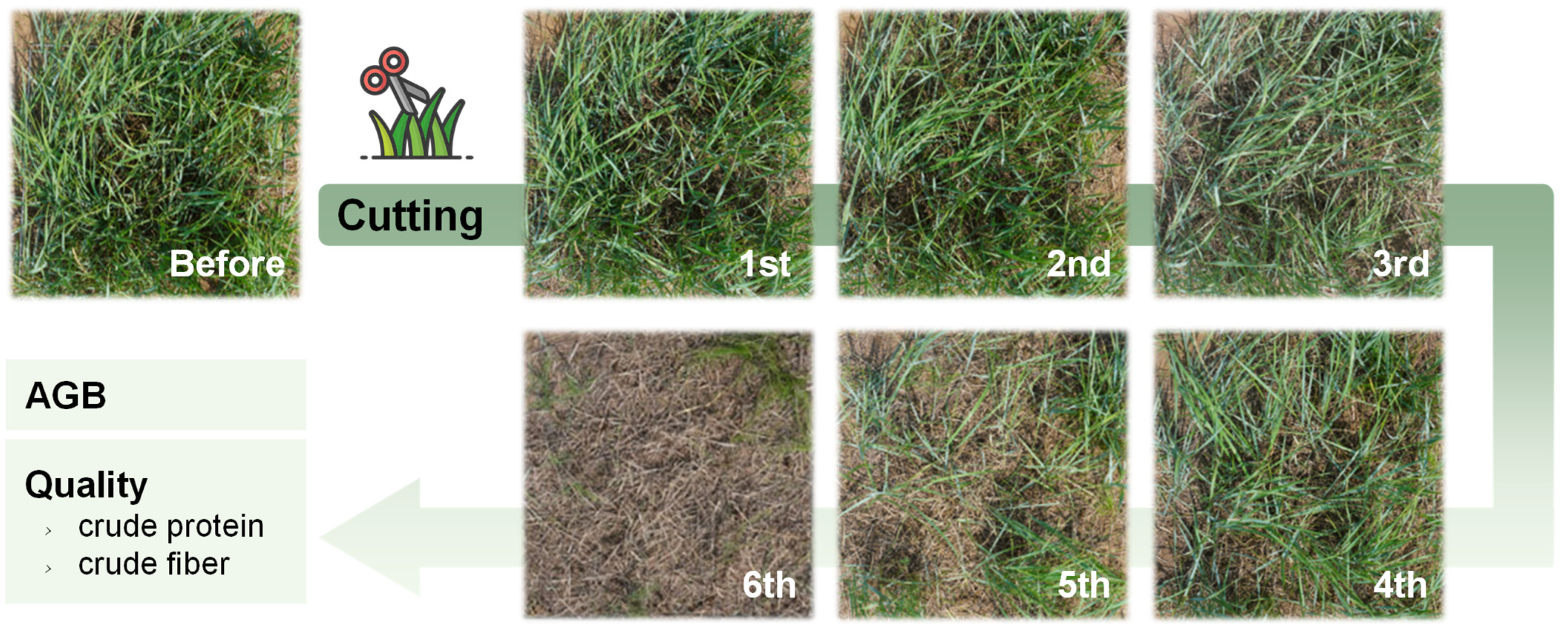
2.2. Gradient Grass-Cutting Experiments and Field Measurements

To facilitate a quick establishment of models to predict forage biomass, CFarea, and CParea, we conducted gradient grass-cutting experiments at 19 sites during the peak growing season in August 2021 (Table S1). At each replicated site (3–6 replicates for each community type), we selected one 10 m × 10 m plot within a larger homogeneous area. In each plot, one 60 cm × 60 cm quadrat was randomly selected to conduct the gradient grass-cutting experiments. Plant shoots were cut randomly with scissors to create 5 to 8 gradients of vegetation coverage until all the aboveground biomass was removed (see an example in Figure 2 and Figure S1). The amount of cutting in each quadrat depended on the initial vegetation coverage in the quadrat (Table S1). The removed biomass of each cutting was labelled separately for further measurements of dry mass and forage quality in the laboratory. Other information, including the latitude, longitude, elevation, plant species, and coverage, was recorded simultaneously.
In each quadrat, ground-based spectral reflectance was measured separately for the initial status and after each cutting under clear sky conditions. Spectral measurements were conducted using an SR-5400 Hi-Res Portable Spectroradiometer (Spectral Evolution Inc., Lawrence, MA, USA) that can detect a light spectral range from 350 to 2500 nm. The spectrometer collects data at 2.5 nm, 5.5 nm, and 5.8 nm sampling interval in the 350–700 nm, 700–1500 nm, and 1500–2500 nm spectral regions, respectively. The spectral data were obtained at a 1 nm spectral interval. Prior to each spectral measurement, a calibration was conducted using a white reference panel, and thus the measured data represented the absolute reflectance. Spectral measurements were conducted at ca. 1.50 m above the grassland canopy for an area of 60 cm × 60 cm. The device was set to automatically conduct ten single measurements and average these measurements into one reflectance curve for further analysis. Low-quality data due to bad weather (e.g., windy or cloudy) or instrument failures were removed prior to further analysis.

2.3. Laboratory Measurements of Forage Biomass and Quality

The plant samples were oven-dried at 65 °C for 72 h, weighed, and ground. Concentration of forage crude protein was quantified by multiplying N concentrations by 6.25 (reference to a national standard GB/T6432-2018, General administration of quality supervision, People’s Republic of China). N concentration was measured using an elemental analyzer (vario MACRO cube, Elementar, Germany). Concentrations of crude fiber were measured using an automatic fiber analyzer (ANKOM 2000i, ANKOM Technology, Macedon, NY, USA). The forage biomass (g m−2) before each cutting was calculated as the summed dry mass of all following cuttings. The amounts of CFarea and CParea (g m−2) were calculated based on forage biomass and corresponding concentrations of crude fiber and crude protein, respectively.

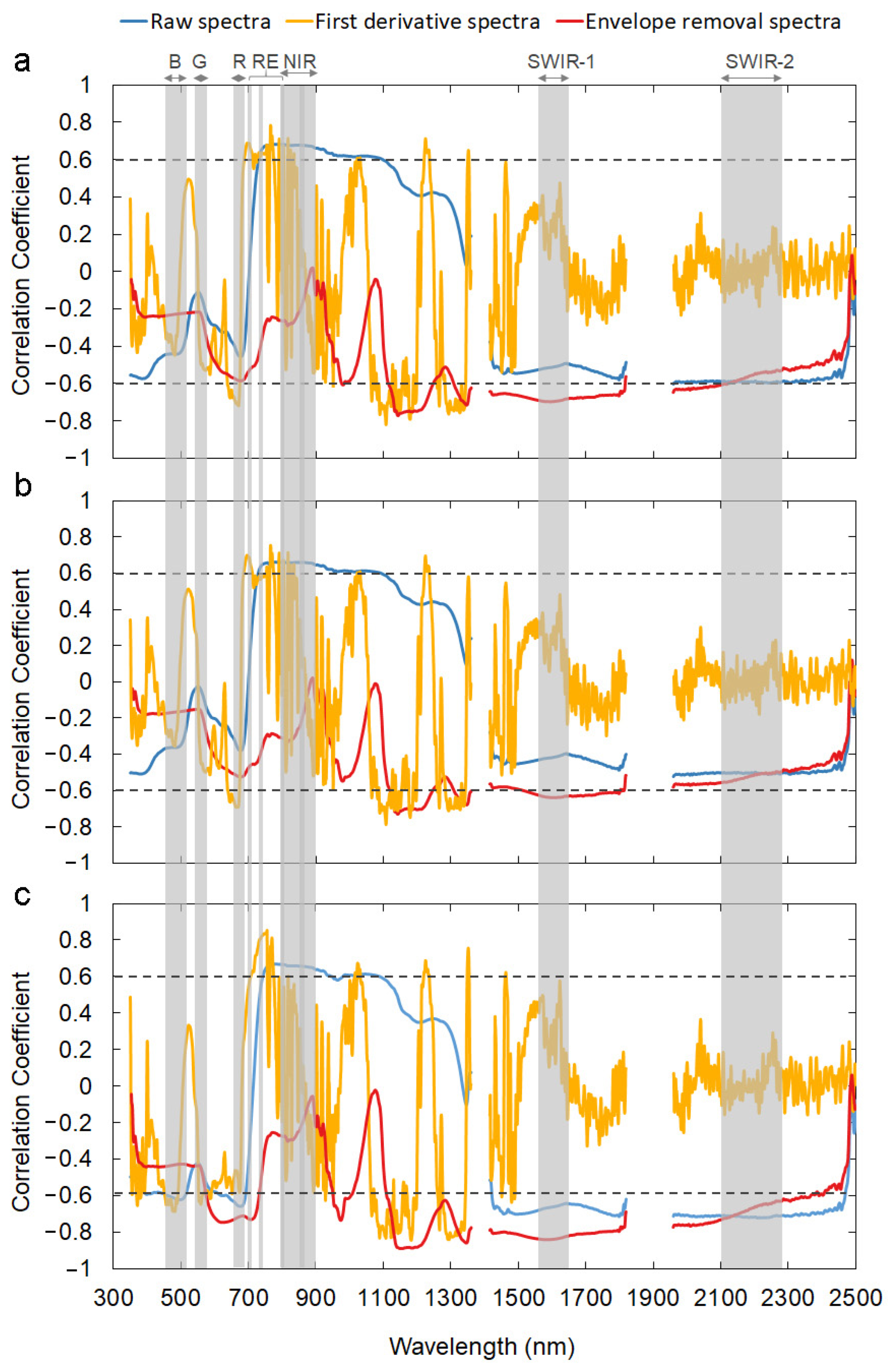
2.4. Identifying Sensitive Spectral Bands

We conducted an analyses of ground-measured spectral data to identify the sensitive spectral bands, which further helped to select potential spectral indices for model construction (See Section 2.5). Raw spectrum reflectance data were preprocessed before further analysis. Two water vapor absorption bands (1400 nm and 1900 nm) were first removed due to strong noise. Random noises were further eliminated by Savitzky-Golay (SG) filtering to derive denoised raw spectral curves of each measurement [30]. Previous studies showed that, compared with the raw spectral reflectance, the first derivative transformation of spectrum can reduce or eliminate the influence of background and atmospheric scattering and thus improve the contrast of different spectral absorption features [14]. In addition, the envelope elimination method can effectively strengthen the absorption and reflection characteristics of spectral curves and normalize data to a consistent spectral background, thereby improving the comparison of eigenvalues with other spectral curves [31]. Therefore, derivative transformation and envelope removal were conducted for the denoised spectral curves. Correlation analyses with forage biomass and quality were conducted separately using raw, derivative transformed, and envelope removal spectral data. The sensitive bands were further recognized based on the correlations (r > 0.6) between spectral reflectance and forage biomass, CFarea, and CParea, respectively.

2.5. Empirical Models for Forage Biomass and Quality Predictions

Nine spectral indices (Table 1) were selected as potential predictors of forage biomass and quality based on three criteria. First, the spectral indices were derived from sensitive spectral bands (see Section 2.4). Second, the spectral indices were theoretically indicative of forage biomass and/or quality-based previous studies (Table 1). Third, only common bands of ground-measured and S2 reflectance were used for the analysis. Field in situ measured data of spectral reflectance were resampled to the S2 spectral configuration. The average reflectance values of corresponding bands were calculated according to S2 wavelength (Table S2) and further used to calculate the nine spectral indices, including NDVI, EVI, NDVI705, REIP, IRECI, NDRE, NRI, NGI, and LSWI (see more details in Table 1).
Two modelling approaches were used to predict forage biomass, CFarea, and CParea. Machine learning algorithms such as Random Forest (RF) analyses have been successfully applied to develop spatially explicit estimates of forage biomass and quality [16,22,32]. We first conducted RF model analyses using all nine spectral indices as predictors [33]. The permutation-based variable importance for each predictor was estimated as the reduction in Root-Mean-Square Error (RMSE) [34,35]. We further conducted regression model analyses using the most important predictor identified by the RF model analyses. Model accuracies of the regression models were estimated using the Leave-One-Out Cross Validation (LOOCV) approach and reported as the coefficient of determination (R2), the Root Mean-Square Error (RMSE) and Normalized Root Mean Squared Error (NRMSE), respectively [36]. The LOOCV approach is a special case of k-fold cross-validation that divides the raw data into k (k = n, n is the number of samples) training subsets of equal size, and the overall accuracy is calculated as the average of the accuracy values computed for each subset. It has been widely used to estimate model accuracies, especially for data of a small sample size [37,38,39]. The model accuracies of the RF models and regression models were further compared. We aim to derive regression models with good accuracies because they are easier to use for monitoring and management purposes.
Table 1. Indices used as potential predictors of forage biomass and quality.
IndicesNameAbbrev. Calculation FormulaReference
Vegetation indicesNormalized Difference Vegetation IndexNDVI (NIR − R)/(NIR + R)[40]
Enhanced Vegetation IndexEVI NIR R NIR + 6   ×   R 7.5   ×   B + 1   ×   2.5 [41]
Indices with red-edge wavelengthsRed Edge Normalized Difference Vegetation IndexNDVI705(RE1 − RE2)/(RE1 + RE2)[42]
Red-Edge Inflection PointREIP 705 + 35 × R + RE 3 2 RE 1 R E 2 R E 1 [43]
Inverted Red-Edge Chlorophyll Index algorithmIRECI RE 3 R RE 1 / RE 2 [44]
Normalized Difference Red Edge indexNDRE(NIR2 − RE2)/(NIR2 +RE2)[45]
Indices with green wavelengthNitrogen Reflectance IndexNRI(G − R)/(G + R)[46]
Normalized Greenness IndexNGI(RE2 − G)/(RE2 + G)[47]
Moisture sensitive indexLand Surface Water IndexLSWI(SWIR − NIR)/(SWIR + NIR)[48]
Note: B represents the blue band (band 2 of Sentinel-2), G represents the green band (band 3 of Sentinel-2), NIR and NIR2 represent the near-infrared bands (band 8 and band 8A of Sentinel-2), R represents the red band (band 4 of Sentinel-2), RE1, RE2, and RE3 represent the three vegetation red edge bands (band 5, band 6, and band 7 of Sentinel-2), SWIR represents the shortwave infrared band (band 12 of Sentinel-2).

2.6. Mapping Forage Biomass and Quality, and Livestock Carrying Capacity

For large-scale mapping, we used S2 data as previous studies have shown that models developed based on spectroradiometer data, resampling to the S2 configuration, can coincide well with S2 images [49]. Because S2 data only reported averages for each band number, we thus calculated average reflectance values of corresponding bands according to S2 Wavelength (Table S2). Our results showed that the spec-field LSWI agreed well with S2 LSWI data (r = 0.52, p = 0.02) (Figure S2), further guaranteeing that these two datasets could be combined to perform reliable predictions of forage status. We collected all the available S2 L2A data (spatial resolution 10 m) within a temporal window of 7 days before the sampling period (1–7 August 2021) from the Google Earth Engine (GEE) platform. Images with cloud and cloud-shadow contamination were removed, and finally two images on 31 July 2021 (S2-B) and 2 August 2021 (S2-A) were selected for the analysis in this study. Based on the empirical regression models in Section 2.5 and corresponding S2 images, we mapped the forage biomass, CFarea, and CParea. We used the empirical regression model because it is easier for practical application and only showed slightly weaker performance than RF models (see Section 3.2). We further analyzed the relationships between predicted forage biomass, CFarea, and CParea and climate variables, including mean annual precipitation (MAP) and mean annual temperature (MAT). MAP and MAT data were obtained from meteorological stations of the China Meteorological Administration and were interpolated to grid cells with a spatial resolution of 10 km using ANUSPLINE software [50].
In the study area, forage was only harvested once a year in the temperate grassland areas. The stocks of peak biomass, CFarea, and CParea can thus roughly indicate the annual forage production, which can be further used to estimate carrying capacity [24]. Biomass alone is not exactly indicative of edible feed for herbivores as the quality of the feed is also an important determinant of grassland carrying capacity [51]. In this study, the livestock carrying capacity was estimated using the predicted forage biomass and CParea. Based on a national standard sheep unit conversion of grass-fed livestock, an animal units (AU) refers to sheep with a mass of 50 kg that consume 1.4 kg of dry matter (forage biomass) and 182 g crude protein per day (reference to the national standard NY/T635-2015 and NY/T3647-2020; Ministry of Agriculture and Rural affairs of the People’s Republic of China). Livestock carrying capacity was then calculated by forage biomass and CParea divided into annual herbage consumption per AU. All statistical analyses were conducted in MATLAB for Windows (Version 2016b, The MathWorks, Inc., Natick, MA, USA) and ArcGIS (Version 10.7, ESRI, Inc., Redlands, CA, USA).

3. Results

3.1. Sensitive Spectral Bands for Forage Biomass and Quality Predictions

Vegetation coverage prior to grass-cutting experiments ranged from 45% to 90% (mean ± sd: 62 ± 13%) across the nineteen plots. Forage biomass, CFarea, and CParea ranged from 179 to 996 (411 ± 194) g m−2, 53 to 366 (128 ± 71) g m−2, and 18 to 88 (42 ± 18) g m−2, respectively (Table S1). Generally, five to eight cuttings were conducted in each quadrat, creating six to nine gradients of vegetation coverage (Table S1). The gradient grass-cutting experiments created clear changes in spectral reflectance after each cutting (Figure S3).
The correlation coefficients for forage biomass, CFarea, and CParea varied across spectrum wavebands. One or more of the three spectrum (raw spectra, first derivative spectra, and envelope removal spectra) showed high correlation coefficients (r > 0.6, p < 0.01) with forage biomass, CFarea, and CParea in the red (650–680 nm), red-edge (698–713 nm, 733–748 nm, 773–793 nm), near-infrared (NIR, 785–900 nm), and short-wave infrared bands (SWIR, 1565–1655 nm and 2100–2280 nm) (Figure 3).The correlation was weak for forage biomass and CFarea in the blue (458–523 nm) and green bands (543–578 nm), while it was fairly strong for CParea. Compared with forage biomass and CFarea, CParea showed stronger correlations with raw spectra, in both the red and SWIR bands, while the correlation coefficients for all these three variables were similar in the NIR region (Figure 3a–c). Similarly, compared with forage biomass and CFarea, CParea showed a stronger correlation with the first derivative spectra in the red band and parts of the NIR bands, and a stronger correlation with the envelope removal spectra in the SWIR bands (Figure 3a–c). Based on the analysis of sensitive spectra bands, we selected nine spectral indices as potential predictors for forage biomass, CFarea, and CParea, including two vegetation indices, four indices with red-edge bands, two indices with a green band, and one moisture-sensitive index (LSWI) (see Section 2.5; Table 1).

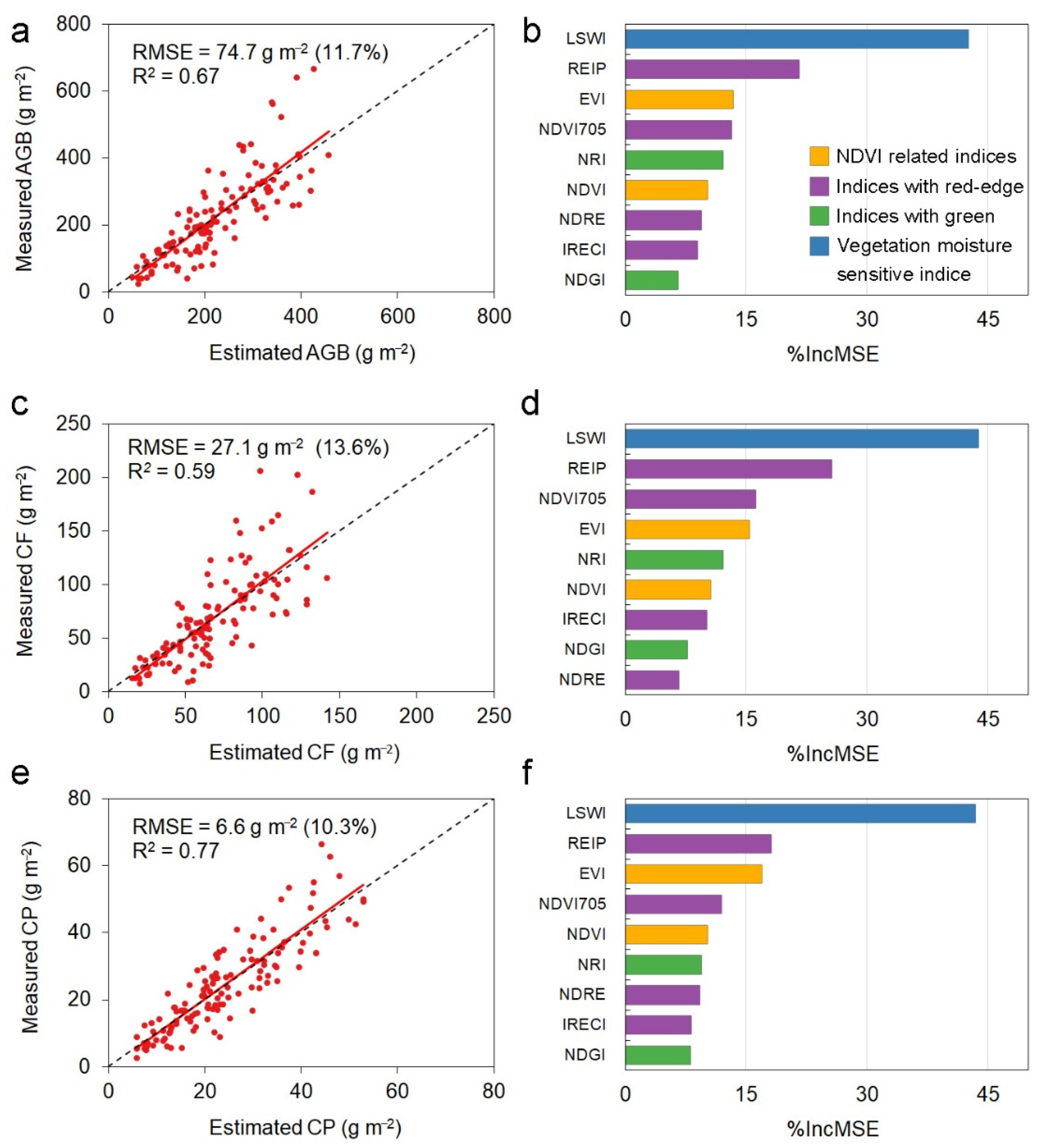
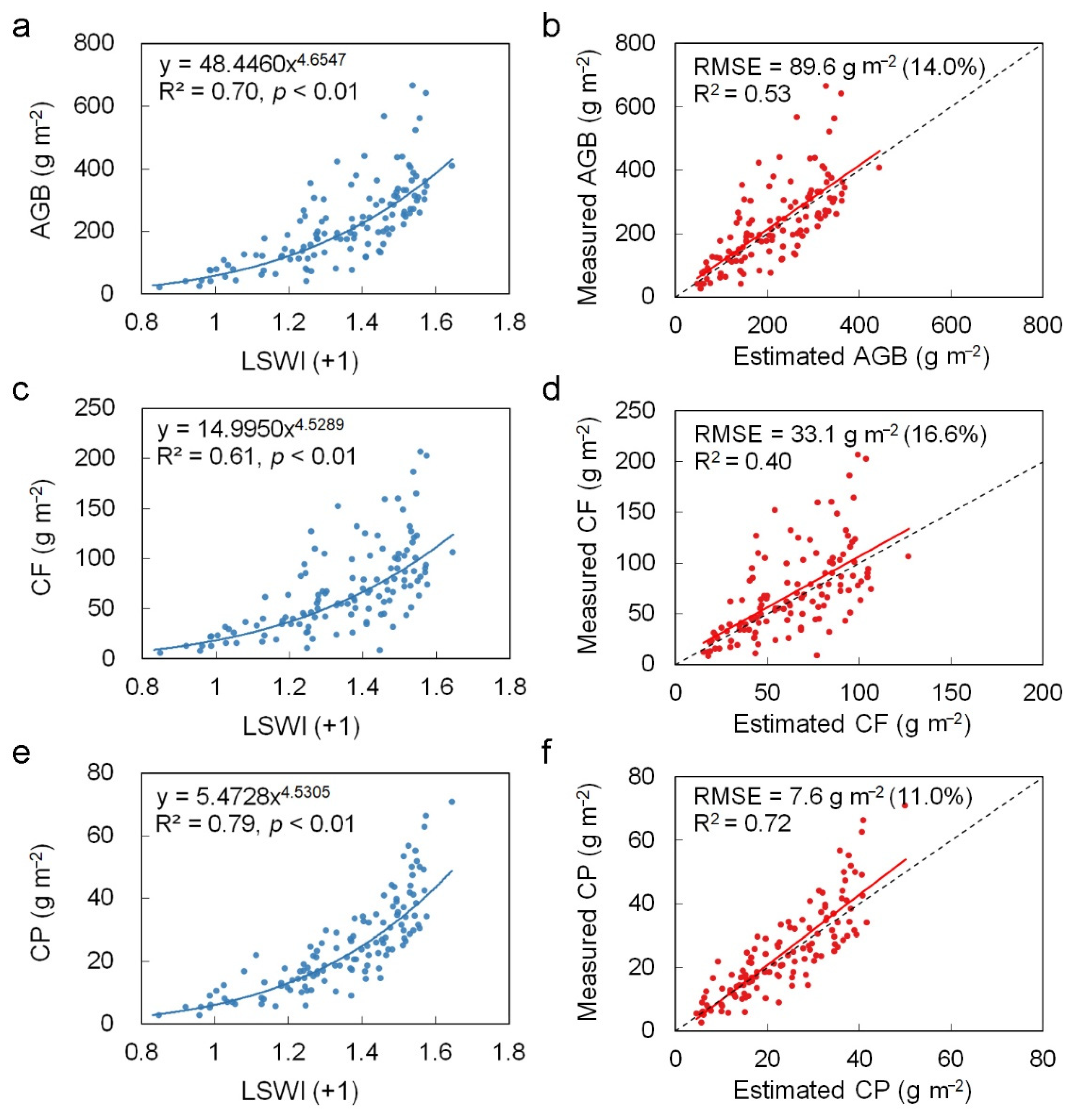
3.2. Performances of Random Forest Models and Power Law Models

Random Forest models using all nine indices well predicted forage biomass (R2 = 0.67, RMSE = 74.7 g m−2), crude fiber (R2 = 0.59, RMSE = 27.1 g m−2), and crude protein per area (R2 = 0.77, RMSE = 6.6 g m−2) (Figure 4a,c,e). Intriguingly, LSWI was the most important predictor for all three models (Figure 4b,d,f), implying a potential approach that simply uses LSWI to predict forage biomass, CFarea, and CParea. Our further analysis showed that forage biomass (R2 = 0.70, p < 0.01), CFarea (R2 = 0.61, p < 0.01), and CParea (R2 = 0.79, p < 0.01) all increased significantly with LSWI in the form of a power law model (Figure 5a,c,e). The power law models well predicted the forage biomass (RMSE = 91.9 g m−2), crude fiber (RMSE = 33.1 g m−2), and crude protein per area (RMSE = 7.6 g m−2) (Figure 5b,d,f). The Random Forest and power law models both predicted CParea better than forage biomass and CFarea (Figure 4 and Figure 5). Although the power law models showed slightly lower prediction accuracies than those of the Forest models, the power law models using LSWI as the single predictor has an advantage for a rapid assessment of regional forage status. An additional analysis showed that residuals of power law models showed no significant difference from 0, implying no overestimation or underestimation of the measured values (forage biomass, p = 0.87; CParea, p = 0.88; CFarea, p = 0.84).

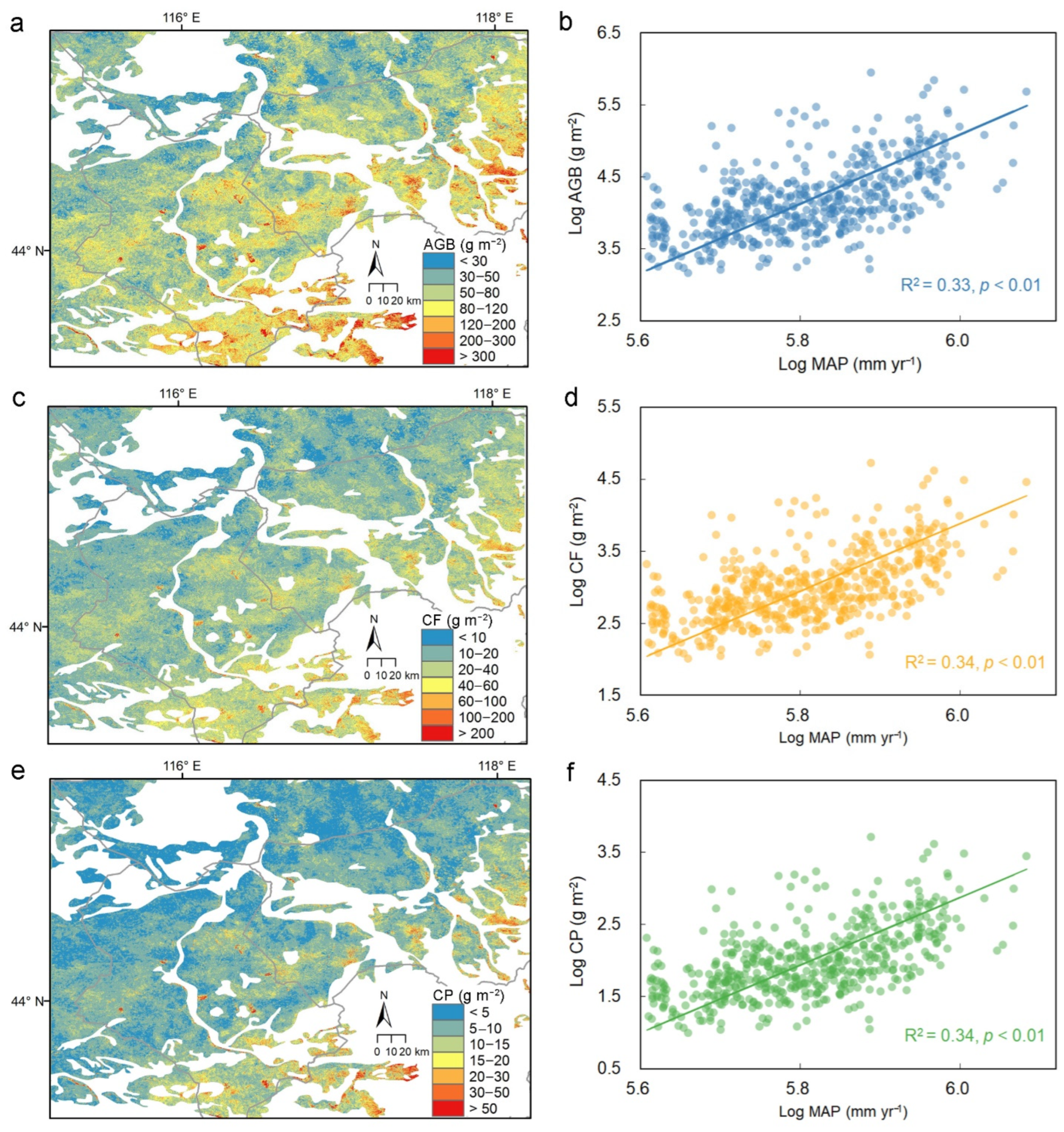
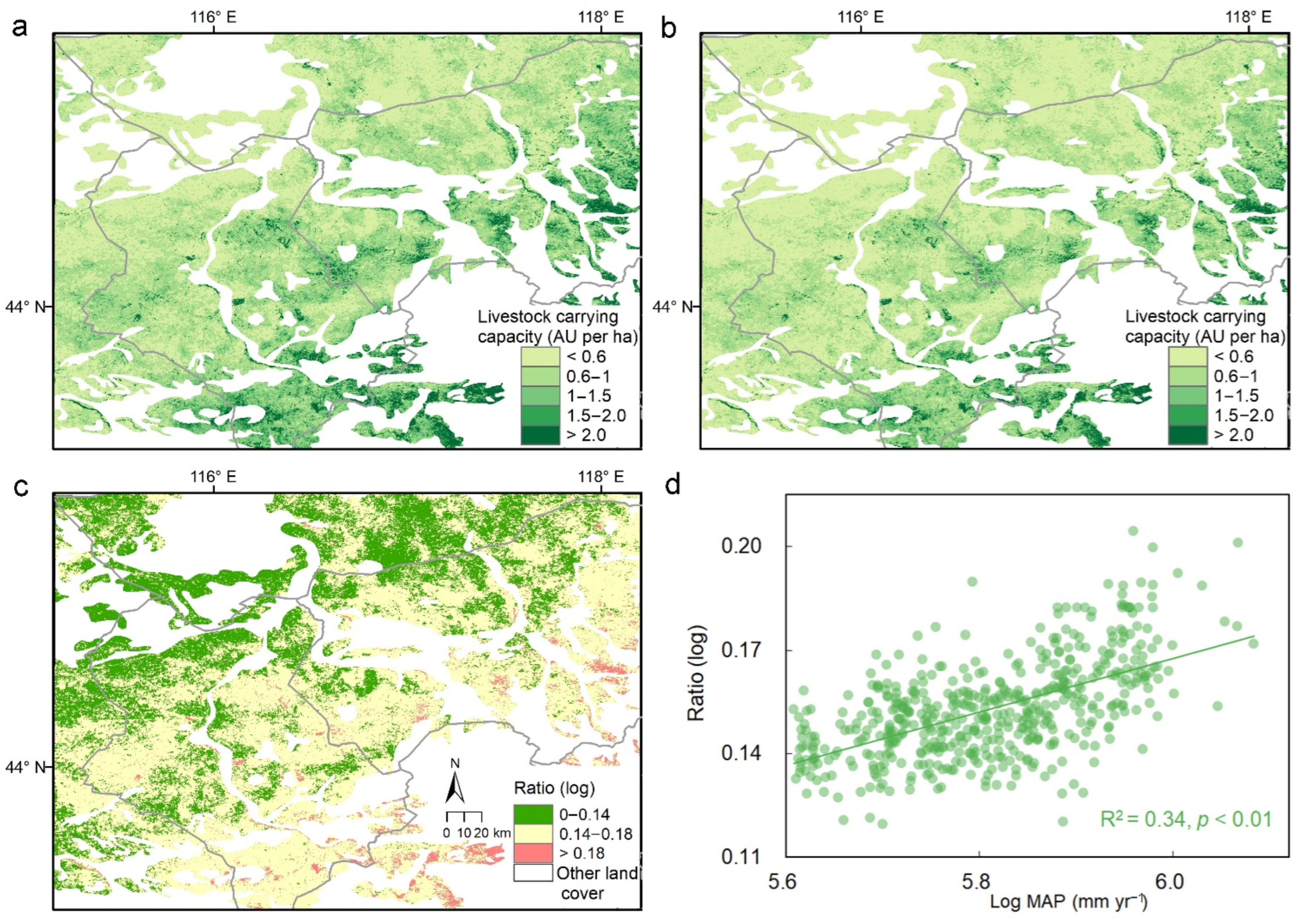
3.3. Regional Patterns of Forage Status and Livestock Carrying Capacity

Using the empirical power law models and corresponding LSWIs calculated from S2 imagery, we separately mapped the forage biomass, CFarea, and CParea in the study area (Figure 6a,c,e). Forage biomass, CFarea, and CParea all showed lower values in the northwest and higher values in the southeast (Figure 6a,c,e), being significantly correlated with MAP (R2 = 0.34, p < 0.01; Figure 6b,d,f), but showed a weak correlation with MAT (R2 = 0.02, p < 0.01; Figure S4a). The average of forage biomass, CFarea, and CParea in the study area were 75.5 ± 61.8 g m−2, 23.0 ± 18.0 g m−2, and 8.38 ± 6.59 g m−2, respectively.
The estimates of livestock carrying capacity based on forage biomass and crude protein showed similar spatial patterns (Figure 7a,b). However, livestock carrying capacity was generally overestimated when using forage biomass in comparison with estimates based on crude protein (1.46 ± 1.32 vs. 1.25 ± 0.93 AU per ha). This overestimation showed significant spatial heterogeneity: it was overestimated by 12–15% in the northwest region with a drier climate, while it was overestimated by more than 20% in the southeast region with wetter climate (Figure 7c). Overall, the ratio of livestock carrying capacity based on forage biomass versus that based on crude protein increased significantly with MAP (R2 = 0.34, p < 0.01; Figure 7d) but only showed weak correlation with MAT (R2 = 0.03, p < 0.01; Figure S4b).

4. Discussion

4.1. Sensitive Spectral Bands and Spectral Indices for Forage Status

Our analysis showed that the spectra of the red-edge, NIR, and SWIR bands were significantly correlated with forage biomass and quality. Similarly, previous work in New Zealand temperate grasslands [14] and in highly diverse Mediterranean permanent grasslands [16] found that the spectra of the red-edge and SWIR bands were the best predictors of CParea. Compared with the first derivative spectra and envelope removal spectra, which can only be calculated from hyperspectral data, we found that the raw spectra in the NIR and SWIR bands (especially 2100–2280 nm) correlated well with forage biomass and quality. These correlations suggest that it is possible to use multispectral datasets to assess forage biomass and quality. Recent studies have explored the potential of S2 multispectral data to assess grassland biomass [22,52] and pasture quality [16,53]. The results showed that the spectra of the red-edge bands from S2 with fine resolutions (10-m) offer an unprecedented opportunity to predict forage quality [23]. In accordance with those previous studies, our results demonstrate that predicted forage biomass using in situ S2 bands resampled from field spectral data agreed well with observed values (LOOCV mean R t e s t 2 = 0.67, NRMSE = 11.7%) (Figure 4a). The prediction of forage quality also showed high accuracy (CFarea: LOOCV mean R t e s t 2 = 0.59, NRMSE = 13.6%; CParea: LOOCV mean R t e s t 2 = 0.77, NRMSE = 10.3%) (Figure 4c,e).
In particular, the LSWI with the spectral information from NIR and SWIR regions was found to be the most important predictor of forage biomass and quality. We further compared the empirical power law models using LSWI alone with the RF models. The results suggested that the empirical power law models showed comparable performance for predicting forage biomass and quality, with slighter accuracies (biomass: NRMSE = 14.0%; CFarea: NRMSE = 16.6%; CParea: NRMSE = 11.0%) than that of the RF models using nine spectral indices. This result suggests that spectral information from NIR and SWIR regions is optimal for retrieving forage biomass and quality. A recent study in a wet region (MAP = 1200 mm) also suggests that LSWI was the optimum index to determine fescue plant health as compared with NDVI and EVI, especially during dry years [54]. The good performance of prediction may be attributable to the fact that SWIR bands contain critical information for canopy N% and leaf water content estimation, while spectral features from the NIR region might have advantages to disentangle canopy structural characteristics [55,56].

4.2. Better Prediction of Forage Protein Than Biomass and Forage Fiber

Random Forest models and the empirical power law models both predicted CParea better than forage biomass and CFarea (Figure 4 and Figure 5). Many studies have reported that the VIS-NIR spectral region correlates well with the CP concentration that is usually estimated from total N concentration in forages [14,15,57]. In view of the fact that the photosynthetic enzymes, especially Rubisco, are major N-containing biochemical constituent within the leaf cells [58], leaf N shows a strong correlation with chlorophyll content that can be reflected by the NIR spectral regions. Moreover, proteins can also be reflected using the SWIR bands [12,13,14] due to the absorption characteristics of protein-associated X-H bonds in the SWIR regions [10]. Therefore, foliar traits related to leaf biochemical and photosynthetic processes could be better estimated and mapped using optical remote sensing data [59]. However, it should be noted that the relationship between canopy chlorophyll content and N decreased in the reproductive growth stage, which limits the capability of estimating N from chlorophylls at the end of the growing seasons [12,60].
Furthermore, LSWI was initially proposed to indicate vegetation liquid water content [61] and vegetation water stress based on the water absorbing SWIR bands [48]. Because LSWI correlates well with both vegetation liquid water content and soil moisture content, it might well capture changes in vegetation healthy signals, especially in dryland systems due to lower soil moisture [62]. Our results suggest that CParea is retrieved more accurately from LSWI than from other vegetation indices (Figure 4f), potentially because it is sensitive to leaf water stress, which limits the leaf biochemical process and loss of leaf N concentration [63].

4.3. Regional Mapping of Forage Status and Management Implications

As discussed above, satellite images at a coarser resolution than in situ measurements can provide information for mapping forage biomass and quality at large spatial scales [10,49]. We first established empirical models using field canopy reflectance resampled to the S2 configuration and then applied these models to S2 images for regional mapping of forage biomass and quality. The rank correlation analysis illustrated that both datasets, Spec-field and S2 LSWI, showed good consistency (r = 0.52, p = 0.02) (Figure S2), which confirmed that these two datasets could be combined to perform the reliable predictions of forage status. Our estimates of forage biomass, CFarea, and CParea agree well with previous assessments based on field sampling in the study area [64].
The spatial distribution of forage biomass, CFarea, and CParea across the research area appeared similar due to intrinsic correlations among these variables (Figure 6a,c,e). In view that plant growth in grasslands is limited by precipitation [65], spatial variations in forage status were significantly associated with changes in precipitation (Figure 6b,d,f). Although spatial heterogeneity in forage quality can be affected by micro-topography [10,20] or field management [16] at a local scale, it was significantly controlled by annual precipitation at large scales in temperate arid grasslands, where precipitation was the major limiting factor [66]. Compared to CP content expressed in mass units (%), our study focused on the estimation of CParea, which was upscaled as the total mass of protein on an area basis and was more suitable for management purposes [12,28].
Livestock carrying capacity is conventionally assessed based on forage biomass production, while forage quality (e.g., CParea) is rarely considered, despite its importance for animal nutrition [2]. Integrating information on forage quality might provide a more reasonable estimation for livestock carrying capacity [3,18]. By comparing estimates separately based on forage biomass and crude protein, we found that livestock carrying capacity was consistently overestimated, and the overestimation was higher in regions with wetter climates (Figure 7). As metabolizable energy could be the limiting factor determining the carrying capacity, we thus calculated the carrying capacity based on local estimate of metabolizable energy from Shi et al. (2013) and found that the result (1.27 AU per ha) was similar to our estimate from CP (1.25 AU per ha) (Table S6). However, the estimate of carrying capacity based on forage biomass was much higher (1.46 AU per ha). These results further confirm that our prediction of carrying capacity based on CP is more reasonable than that based on forage biomass in the study area. Therefore, the risk of overgrazing will likely increase when using the conventional estimates of livestock carrying capacity based on forage biomass to guide local livestock management.

4.4. Uncertainties and Future Research Needs

The regional mapping of forage status conventionally replies on empirical models established from a labor-intensive and time-consuming field survey across large-scale natural gradients in combination with satellite observations [14,16,19,20]. A more cost-effective and easy-to-use approach is thus needed for the rapid assessment of forage status and livestock management. To this end, we conducted novel gradient grass-cutting experiments at a small number of sites to facilitate a quick establishment of models to map regional forage production and quality. Despite the good performance of prediction, possible uncertainties likely remain in our study. For example, there might be a potential effect of autocorrelation due to gradient cuttings at each site. Additional analyses indicate that grass-cutting had insignificant interactions with site and LSWI, implying that the potential autocorrelation would not strongly influence the robustness of our models (Tables S3–S5). The optimal prediction models established in this study may also be limited to the temperate grasslands (e.g., Xilingol region), where plant growth is limited by precipitation. It remains to be tested whether such models are applicable to the regions dominated by temperature and other factors. Moreover, the spectral indices obtained from canopy reflectance can be influenced by soil background conditions. Our further analysis showed no significant difference between the LWSI obtained by canopy reflectance and the corrected LWSI without soil background (p = 0.59) (Figure S5). Additionally, there could be differences between LSWI values calculated from in situ measurements and satellite observations. This difference might result in uncertainties when applying models for regional mapping. To reduce such uncertainties, we established the empirical models using field canopy reflectance resampled to the S2 configuration. A correlation analysis also showed that both datasets, spec-field and S2 LSWI, showed good consistency (Figure S2), further confirming that these two datasets could be combined to perform reliable predictions of forage status.

5. Conclusions

By conducting novel gradient grass-cutting experiments and corresponding ground-based measurements in temperate grasslands in Inner Mongolia, we evaluated sensitive spectral bands, derived nine potential spectral indices, and established Random Forest models that well predicted forage biomass, CFarea, and CParea. LSWI was found to be the most important predictor, and empirical power law models using LSWI alone showed comparable prediction accuracies to the Random Forest models. Regional patterns of forage biomass and quality were thus mapped by combining the empirical power law models with LSWI calculated from S2 observations. The predicted forage biomass, CFarea, and CParea all showed a strong increase with mean annual precipitation. Livestock carrying capacity was overestimated based on forage biomass in comparison to the estimates using crude protein, implying a risk of overgrazing in regional grasslands when using conventional estimates for livestock management guidance. These approaches provide useful tools to simultaneously map the forage biomass and quality metrics using remote sensing data, and the LSWI-based power models can be used for a rapid assessment of forage status to support livestock management.

Supplementary Materials

The following supporting information can be downloaded at: https://www.mdpi.com/article/10.3390/rs15081973/s1, Table S1: A summary of initial vegetation status and gradient-cutting experiments of all 19 grassland sites. Table S2: Spectral specifications of the Sentinel-2 MSI instrument. Table S3: A summary of multiple regression analysis for forage biomass. Table S4: A summary of multiple regression analysis for forage CFarea. Table S5: A summary of multiple regression analysis for forage CParea. Table S6: Livestock carrying capacity (AU per ha) estimated using forage biomass (DM), crude protein (CP), and the metabolizable energy (ME) respectively. Figure S1: The amount of grass biomass (above-ground biomass, AGB) corresponding to each grass-cutting in an example quadrat. Figure S2: Correlations between LSWI retrieved from field spectral data and in-situ S2 dataset (2021/07/31) for 19 sampling plots. Figure S3: An example of spectral changes after each grass-cutting. Figure S4: Changes in predicted forage biomass, CFarea and CParea (a) and the ratio between biomass based and CParea based carrying capacity (b) with mean annual temperature (MAT). Figure S5: Correlations between LSWI retrieved from canopy reflectance with soil background (LSWI) and without soil background (LSWIveg) for 19 sampling plots.

Author Contributions

X.Z. designed the study; X.Z., B.W. and J.X. collected and analyzed the data; X.Z., Y.S., M.Z., X.G., Z.Y., H.S. and J.F. wrote the manuscript. All authors have read and agreed to the published version of the manuscript.

Funding

This work is supported by the National Natural Science Foundation of China (grant no. 32071881), the Special Project for Social Development of Yunnan Province to M.Y. (grant no. 202103 AC100001), and the Strategic Priority Research Program of the Chinese Academy of Sciences (grant no. XDA26010303).

Data Availability Statement

All data included in this study are available upon request by contact with the corresponding author.

Acknowledgments

We are grateful to Yinpin Feng, Yingjie Dong, and Jianjun Chen for their help in data collection.

Conflicts of Interest

The authors declare that they have no conflict of interest.

References

  1. O’Mara, F.P. The role of grasslands in food security and climate change. Ann. Bot. 2012, 110, 1263–1270. [Google Scholar] [CrossRef] [Green Version]
  2. Piipponen, J.; Jalava, M.; de Leeuw, J.; Rizayeva, A.; Godde, C.; Cramer, G.; Kummu, M. Global trends in grassland carrying capacity and relative stocking density of livestock. Glob. Chang. Biol. 2022, 28, 3902–3919. [Google Scholar] [CrossRef] [PubMed]
  3. Golluscio, R.A.; Bottaro, H.S.; Oesterheld, M. Controls of carrying capacity: Degradation, primary production, and forage quality effects in a Patagonian steppe. Rangel. Ecol. Manag. 2015, 68, 266–275. [Google Scholar] [CrossRef]
  4. Schellberg, J.; Hill, M.J.; Gerhards, R.; Rothmund, M.; Braun, M. Precision agriculture on grassland: Applications, perspectives and constraints. Eur. J. Agron. 2008, 29, 59–71. [Google Scholar] [CrossRef]
  5. De Leeuw, J.; Vrieling, A.; Shee, A.; Atzberger, C.; Hadgu, K.M.; Biradar, C.M.; Turvey, C. The potential and uptake of remote sensing in insurance: A review. Remote Sens. 2014, 6, 10888–10912. [Google Scholar] [CrossRef] [Green Version]
  6. Piao, S.; Mohammat, A.; Fang, J.; Cai, Q.; Feng, J. NDVI-based increase in growth of temperate grasslands and its responses to climate changes in China. Glob. Environ. Chang. 2006, 16, 340–348. [Google Scholar] [CrossRef]
  7. Ali, I.; Cawkwell, F.; Dwyer, E.; Barrett, B.; Green, S. Satellite remote sensing of grasslands: From observation to management. J. Plant Ecol. 2016, 9, 649–671. [Google Scholar] [CrossRef] [Green Version]
  8. Reinermann, S.; Asam, S.; Kuenzer, C. Remote sensing of grassland production and management—A review. Remote Sens. 2020, 12, 1949. [Google Scholar] [CrossRef]
  9. Zhou, Y.; Liu, T.; Batelaan, O.; Duan, L.; Wang, Y.; Li, X.; Li, M. Spatiotemporal fusion of multi-source remote sensing data for estimating aboveground biomass of grassland. Ecol. Indic. 2023, 146, 109892. [Google Scholar] [CrossRef]
  10. Lugassi, R.; Zaady, E.; Goldshleger, N.; Shoshany, M.; Chudnovsky, A. Spatial and temporal monitoring of pasture ecological quality: Sentinel-2-based estimation of crude protein and neutral detergent fiber contents. Remote Sens. 2019, 11, 799. [Google Scholar] [CrossRef] [Green Version]
  11. Curran, P.J. Remote sensing of foliar chemistry. Remote Sens. Environ. 1989, 30, 271–278. [Google Scholar] [CrossRef]
  12. Berger, K.; Verrelst, J.; Féret, J.B.; Wang, Z.H.; Wocher, M.; Strathmann, M.; Danner, M.; Mauser, W.; Hank, T. Crop nitrogen monitoring: Recent progress and principal developments in the context of imaging spectroscopy missions. Remote Sens. Environ. 2020, 242, 111758. [Google Scholar] [CrossRef] [PubMed]
  13. Pellissier, P.A.; Ollinger, S.V.; Lepine, L.C.; Palace, M.W.; McDowell, W.H. Remote sensing of foliar nitrogen in cultivated grasslands of human dominated landscapes. Remote Sens. Environ. 2015, 167, 88–97. [Google Scholar] [CrossRef] [Green Version]
  14. Pullanagari, R.R.; Dehghan-Shoar, M.; Yule, I.J.; Bhatia, N. Field spectroscopy of canopy nitrogen concentration in temperate grasslands using a convolutional neural network. Remote Sens. Environ. 2021, 257, 112353. [Google Scholar] [CrossRef]
  15. Kawamura, K.; Watanabe, N.; Sakanoue, S.; Inoue, Y. Estimating forage biomass and quality in a mixed sown pasture based on PLS regression with waveband selection. Grassl. Sci. 2008, 54, 131–145. [Google Scholar] [CrossRef]
  16. Fernández-Habas, J.; Moreno, A.M.G.; Hidalgo-Fernández, M.A.T.; Leal-Murillo, J.R.; Oar, B.A.; Gámez-Giráldez, P.J.; González-Dugo, M.P.; Fernández-Rebollo, P. Investigating the potential of Sentinel-2 configuration to predict the quality of Mediterranean permanent grasslands in open woodlands. Sci. Total Environ. 2021, 791, 148101. [Google Scholar] [CrossRef]
  17. Clark, D.H.; Lamb, R.C. Near infrared reflectance spectroscopy: A survey of wavelength selection to determine dry matter digestibility. J. Dairy Sci. 1991, 74, 2200–2205. [Google Scholar] [CrossRef]
  18. Wijesingha, J.; Astor, T.; Schulze-Brüninghoff, D.; Wengert, M.; Wachendorf, M. Predicting forage quality of grasslands using UAV-borne imaging spectroscopy. Remote Sens. 2020, 12, 126. [Google Scholar] [CrossRef] [Green Version]
  19. Skidmore, A.K.; Ferwerda, J.G.; Mutanga, O.; Van Wieren, S.E.; Peel, M.; Grant, R.C.; Prins, H.H.T.; Balcik, F.B.; Venus, V. Forage quality of savannas—Simultaneously mapping foliar protein and polyphenols for trees and grass using hyperspectral imagery. Remote Sens. Environ. 2010, 114, 64–72. [Google Scholar] [CrossRef]
  20. Pullanagari, R.; Kereszturi, G.; Yule, I. Integrating airborne hyperspectral, topographic, and soil data for estimating pasture quality using recursive feature elimination with random forest regression. Remote Sens. 2018, 10, 1117. [Google Scholar] [CrossRef] [Green Version]
  21. Zhao, Y.J.; Sun, Y.H.; Lu, X.M.; Zhao, X.Z.; Yang, L.; Sun, Z.Y.; Bai, Y.F. Hyperspectral retrieval of leaf physiological traits and their links to ecosystem productivity in grassland monocultures. Ecol. Indic. 2021, 122, 107267. [Google Scholar] [CrossRef]
  22. Punalekar, S.M.; Verhoef, A.; Quaife, T.L.; Humphries, D.; Bermingham, L.; Reynolds, C.K. Application of Sentinel-2A data for pasture biomass monitoring using a physically based radiative transfer model. Remote Sens. Environ. 2018, 218, 207–220. [Google Scholar] [CrossRef]
  23. Raab, C.; Riesch, F.; Tonn, B.; Barrett, B.; Meißner, M.; Balkenhol, N.; Isselstein, J. Target-oriented habitat and wildlife management: Estimating forage quantity and quality of semi-natural grasslands with Sentinel-1 and Sentinel-2 data. Remote Sens. Ecol. Conserv. 2020, 6, 381–398. [Google Scholar] [CrossRef]
  24. Bai, Y.; Han, X.; Wu, J.; Chen, Z.; Li, L. Ecosystem stability and compensatory effects in the Inner Mongolia grassland. Nature 2004, 431, 181–184. [Google Scholar] [CrossRef]
  25. Hilker, T.; Natsagdorj, E.; Waring, R.H.; Lyapustin, A.; Wang, Y. Satellite observed widespread decline in Mongolian grasslands largely due to overgrazing. Glob. Chang. Biol. 2014, 20, 418–428. [Google Scholar] [CrossRef] [PubMed] [Green Version]
  26. Bai, J.; Shi, H.; Yu, Q.; Xie, Z.; Li, L.; Luo, G.; Li, J. Satellite-observed vegetation stability in response to changes in climate and total water storage in Central Asia. Sci. Total Environ. 2019, 659, 862–871. [Google Scholar] [CrossRef]
  27. Zhao, X.; Shen, H.H.; Geng, X.Q.; Fang, J.Y. Three-decadal destabilization of vegetation activity on the Mongolian Plateau. Environ. Res. Lett. 2021, 16, 034049. [Google Scholar] [CrossRef]
  28. Kattenborn, T.; Schiefer FZarco-Tejada, P.; Schmidtlein, S. Advantages of retrieving pigment content [μg/cm2] versus concentration [%] from canopy reflectance. Remote Sens. Environ. 2019, 230, 111195. [Google Scholar] [CrossRef]
  29. Editorial Committee for Vegetation Atlas of China. Vegetation Atlas of China; Science Press: Beijing, China, 2001. [Google Scholar]
  30. Savitzky, A.; Golay, M.J.E. Smoothing and Differentiation of Data by Simplified Least Squares Procedures. Anal. Chem. 1964, 36, 1627–1639. [Google Scholar] [CrossRef]
  31. Sheng, Q.; Zhang, S.W.; Ge, C.; Liu, H.; Zhou, Y.; Chen, Y.; Hu, Q.; Ye, H.; Huang, Y. Hyperspectral inversion of heavy metal content in soils reconstituted by mining wasteland. Spectrosc. Spectr. Anal. 2019, 39, 1214–1220. [Google Scholar]
  32. Ramoelo, A.; Cho, M.; Mathieu, R.; Skidmore, A.K. Potential of Sentinel-2 spectral configuration to assess rangeland quality. J. Appl. Remote Sens. 2015, 9, 094096. [Google Scholar] [CrossRef] [Green Version]
  33. Breiman, L. Random forests. Mach. Learn. 2001, 45, 5–32. [Google Scholar] [CrossRef] [Green Version]
  34. Strobl, C.; Hothorn, T.; Zeileis, A. Party on! A new, conditional variable importance measure for random forests available in party package. R J. 2009, 1, 14–17. [Google Scholar] [CrossRef]
  35. Strobl, C.; Malley, J.; Tutz, G. An introduction to recursive partitioning: Rationale, application, and characteristics of classification and regression trees, bagging, and random forests. Psychol. Methods 2009, 14, 323–348. [Google Scholar] [CrossRef] [PubMed] [Green Version]
  36. Tramontana, G.; Ichii, K.; Camps-Valls, G.; Tomelleri, E.; Papale, E. Uncertainty analysis of gross primary production upscaling using Random Forests, remote sensing and eddy covariance data. Remote Sens. Environ. 2015, 168, 360–373. [Google Scholar] [CrossRef]
  37. Cawley, G.C.; Talbot, N.L. Efficient leave-one-out cross-validation of kernel fisher discriminant classifiers. Pattern. Recognit. 2003, 36, 2585–2592. [Google Scholar] [CrossRef]
  38. Brovelli, M.A.; Crespi, M.; Fratarcangeli, F.; Giannone, F.; Realini, E. Accuracy assessment of high resolution satelliteimagery orientation by leave-one-out method. ISPRS J Photogramm Remote Sens. 2008, 63, 427–440. [Google Scholar] [CrossRef]
  39. Casella, V.; Chiabrando, F.; Franzini, M.; Manzino, A.M. Accuracy Assessment of a UAV Block by Different Software Packages, Processing Schemes and Validation Strategies. ISPRS Int. J. Geo-Inf. 2020, 9, 164. [Google Scholar] [CrossRef] [Green Version]
  40. Tucker, C.J.; Justice, C.O.; Prince, S.D. Monitoring the grasslands of the Sahel 1984–1985. Int. J. Remote Sens. 1986, 7, 1571–1581. [Google Scholar] [CrossRef]
  41. Huete, A.; Justice, C.; Liu, H. Development of vegetation and soil indices for MODIS-EOS. Remote Sens. Environ. 1994, 49, 224–234. [Google Scholar] [CrossRef]
  42. Cundill, S.L.; van der Werff, H.M.A.; van der Meijde, M. Adjusting spectral indices for spectral response function differences of very high spatial resolution sensors simulated from field spectra. Sensors 2015, 15, 6221–6240. [Google Scholar] [CrossRef] [PubMed]
  43. Herrmann, I.; Pimstein, A.; Karnieli, A.; Cohen, Y.; Alchanatis, V.; Bonfil, D.J. LAI assessment of wheat and potato crops by VENμS and Sentinel-2 bands. Remote Sens. Environ. 2011, 115, 2141–2151. [Google Scholar] [CrossRef]
  44. Frampton, W.J.; Dash, J.; Watmough, G.; Milton, E.J. Evaluating the capabilities of Sentinel-2 for quantitative estimation of biophysical variables in vegetation. ISPRS J Photogramm. Remote Sens. 2013, 82, 83–92. [Google Scholar] [CrossRef] [Green Version]
  45. Thompson, C.N.; Guo, W.X.; Sharma, B.; Ritchie, G.L. Using Normalized Difference Red Edge Index to Assess Maturity in Cotton. Crop Physiol. Metab. 2019, 59, 2167–2177. [Google Scholar] [CrossRef]
  46. Schleicher, T.D.; Bausch, W.C.; Delgado, J.A.; Ayers, P.D. Evaluation and Refinement of the Nitrogen Reflectance Index (NRI) for Site Specific Fertilizer Management. In ASAE Annual International Meeting Report; American Society of Agricultural and Biological Engineers: St. Joseph, MI, USA, 2001. [Google Scholar]
  47. Gitelson, A.A.; Merzlyak, M.N. Signature analysis of leaf reflectance spectra: Algorithm development for remote sending of chlorophyll. J. Plant Physiol. 1996, 148 (Suppl. S3–S4), 494–500. [Google Scholar] [CrossRef]
  48. Xiao, X.; Hollinger, D.; Aber, J.; Goltz, M.; Davidson, E.A.; Zhang, Q.; Moore, B. Satellite-based modeling of gross primary production in an evergreen needleleaf forest. Remote Sens. Environ. 2004, 89, 519–534. [Google Scholar] [CrossRef]
  49. Ramoelo, A.; Cho, M.A. Explaining leaf nitrogen distribution in a semi-arid environment predicted on sentinel-2 imagery using a field spectroscopy derived models. Remote Sens. 2018, 10, 269. [Google Scholar] [CrossRef] [Green Version]
  50. Gu, F.X.; Zhang, Y.D.; Huang, M.; Tao, B.; Liu, Z.; Hao, M.; Guo, R. Climate-driven uncertainties in modeling terrestrial ecosystem net primary productivity in China. Agric. For. Meteorol. 2017, 246, 123–132. [Google Scholar] [CrossRef]
  51. De Leeuw, P.N.; Tothill, J.C. The Concept of Rangeland Carrying Capacity in Sub-Saharan Africa–Myth or Reality; Pastoral Development Network, Overseas Development Institude: London, UK, 1990. [Google Scholar]
  52. Wang, J.; Xiao, X.M.; Bajgain, R.; Starks, P.; Steiner, J.; Doughty, R.B.; Chang, Q. Estimating leaf area index and aboveground biomass of grazing pastures using Sentinel-1, Sentinel-2 and Landsat images. ISPRS J. Photogramm. Remote Sens. 2019, 154, 189–201. [Google Scholar] [CrossRef] [Green Version]
  53. Clevers, J.G.P.W.; Gitelson, A.A. Remote estimation of crop and grass chlorophyll and nitrogen content using red-edge bands on Sentinel-2 and -3. Int J. Appl. Earth. Obs. Geoinf. 2013, 23, 344–351. [Google Scholar] [CrossRef]
  54. Flynn, K.C.; Lee, T.; Endale, D.; Franzluebbers, A.; Ma, S.; Zhou, Y. Assessing Remote Sensing Vegetation Index Sensitivities for Tall Fescue (Schedonorus arundinaceus) Plant Health with Varying Endophyte and Fertilizer Types: A Case for Improving Poultry Manuresheds. Remote Sens. 2021, 13, 521. [Google Scholar] [CrossRef]
  55. Eitel, J.U.H.; Gessler, P.E.; Smith, A.M.S.; Robberecht, R. Suitability of existing and novel spectral indices to remotely detect water stress in Populus spp. For. Ecol. Manag. 2006, 229, 170–182. [Google Scholar] [CrossRef]
  56. DeChant, C.; Wiesner-Hanks, T.; Chen, S.; Stewart, E.L.; Yosinski, J.; Gore, M.A. Automated identification of northern leaf blight-infected maize plants from field imagery using deep learning. Phytopathology 2017, 107, 1426–1432. [Google Scholar] [CrossRef] [PubMed] [Green Version]
  57. Clifton, K.; Bradbury, J.W.; Vehrencamp, S.L. The fine-scale mapping of grassland protein densities. Grass Forage Sci. 1994, 49, 1–8. [Google Scholar] [CrossRef]
  58. Kokaly, R.F.; Asner, G.P.; Ollinger, S.V.; Martin, M.E.; Wessman, C.A. Characterizing canopy biochemistry from imaging spectroscopy and its application to ecosystem studies. Remote Sens. Environ. 2009, 113, S78–S91. [Google Scholar] [CrossRef]
  59. Homolova, L.; Malenovsky, Z.; Clevers, J.G.P.W.; Garcia-Santos, G.; Schaepman, M.E. Review of optical-based remote sensing for plant trait mapping. Ecol. Complex. 2013, 15, 1–16. [Google Scholar] [CrossRef] [Green Version]
  60. Ohyama, T. Nitrogen as a major essential element of plants. In Nitrogen Assimilation in Plants; Ohyama, T., Sueyoshi, K., Eds.; Research Signpost: Trivandrum, India, 2010; pp. 1–18. [Google Scholar]
  61. Gao, B.C. NDWI—A normalized difference water index for remote sensing of vegetation liquid water from space. Remote Sens. Environ. 1996, 58, 257–266. [Google Scholar] [CrossRef]
  62. Kato, A.; Carlson, K.M.; Miura, T. Assessing the inter-annual variability of vegetation phenological events observed from satellite vegetation index time series in dryland sites. Ecol. Indic. 2021, 130, 108042. [Google Scholar] [CrossRef]
  63. Bajgain, R.; Xiao, X.; Wagle, P.; Basara, J.; Zhou, Y. Sensitivity analysis of vegetation indices to drought over two tallgrass prairie sites. ISPRS J. Photogramm. Remote Sens. 2015, 108, 151–160. [Google Scholar] [CrossRef]
  64. Shi, Y.; Ma, Y.; Ma, W.; Liang, C.; Zhao, X.; Fang, J.; He, J. Large scale patterns of forage yield and quality across Chinese grasslands. Chin. Sci. Bull. 2013, 58, 1187–1199. [Google Scholar] [CrossRef] [Green Version]
  65. Hsu, J.S.; Powell, J.; Adler, P.B. Sensitivity of mean annual primary production to precipitation. Glob. Chang. Biol. 2012, 18, 2246–2255. [Google Scholar] [CrossRef]
  66. Ren, H.; Han, G.; Schönbach, P.; Gierus, M.; Taube, F. Forage nutritional characteristics and yield dynamics in a grazed semiarid steppe ecosystem of Inner Mongolia, China. Ecol. Indic. 2016, 60, 460–469. [Google Scholar] [CrossRef]
Figure 1. The study area of temperate grasslands in Xilingol region of IMAR, northern China. Sampling sites with different dominant species are indicated by different colors.
Remotesensing 15 01973 g001
Figure 2. An example of the gradient grass-cutting experiment. The gradual grass-cutting here created seven coverage gradients.
Remotesensing 15 01973 g002
Figure 3. Correlation coefficients for forage biomass (a), crude fiber (CFarea, b) and crude protein per area (CParea, c) with raw spectra (after denoising), first derivative spectra, and envelope removal spectra, respectively. The gray shaded areas indicate the spectral settings and resolutions of S2 images that can be potentially used to estimate forage biomass, CFarea, and CParea. The visible spectra bands (blue: 458–523 nm, green: 543–578 nm, red: 650–680 nm); RE, Red-Edge bands (698–713 nm, 733–748 nm, 773–793 nm); NIR, Near Infrared Bands (785–900 nm); SWIR, Shortwave Infrared Bands (SWIR-1: 1565–1655 nm, SWIR-2: 2100–2280 nm).
Remotesensing 15 01973 g003
Figure 4. Accuracies and predictor importance of Random Forest models for forage biomass (a,b), crude fiber per area (c,d), and crude protein per area (e,f). Percentages in brackets indicate NRMSE. %IncMSE indicates the percent increase in MSE (Mean Squared Error) of predictions as a result of the variable being permuted (values randomly shuffled). Variables with higher %IncMSE values are more important.
Remotesensing 15 01973 g004
Figure 5. Power law models (using LSWI as the predictor) and prediction accuracies for forage biomass (a,b), crude fiber per area (c,d), and crude protein per area (e,f). Note that the independent variable of a power law function cannot be a negative value; we addressed this issue by adding a constant 1 to the LSWI (values ranging from −1 to 1).
Remotesensing 15 01973 g005
Figure 6. Spatial patterns of predicted forage biomass (a), crude fiber (c), and crude protein (e) per area and their correlations with MAP (b,d,f).
Remotesensing 15 01973 g006
Figure 7. Livestock carrying capacity (AU per ha) estimated using forage biomass (a) and crude protein (b), the ratio between these two estimates (c), and shifts of the ratio with MAP (d). AU refers to a national standard sheep with a mass of 50 kg that consumes 1.4 kg of dry matter (forage biomass) and 182 g crude protein per day (reference to the national standard NY/T635-2015 and NY/T3647-2020; Ministry of Agriculture and Rural affairs of the People’s Republic of China). (a,b) has the same scale as in (c).
Remotesensing 15 01973 g007
Disclaimer/Publisher’s Note: The statements, opinions and data contained in all publications are solely those of the individual author(s) and contributor(s) and not of MDPI and/or the editor(s). MDPI and/or the editor(s) disclaim responsibility for any injury to people or property resulting from any ideas, methods, instructions or products referred to in the content.

