Article

An Optimized Workflow for Digital Surface Model Series Generation Based on Historical Aerial Images: Testing and Quality Assessment in the Beach-Dune System of Sa Ràpita-Es Trenc (Mallorca, Spain)

by
Christian Mestre-Runge
1,
Jorge Lorenzo-Lacruz
2,*,
Aaron Ortega-Mclear
3 and
Celso Garcia
3
1
Department of Biology, University of Marburg, 35043 Marburg, Germany
2
Department of Human Sciences, University of La Rioja, 26004 Logroño, Spain
3
Department of Geography, University of the Balearic Islands, 07122 Palma, Spain
*
Author to whom correspondence should be addressed.
Remote Sens. 2023, 15(8), 2044; https://doi.org/10.3390/rs15082044
Submission received: 27 February 2023 / Revised: 3 April 2023 / Accepted: 4 April 2023 / Published: 12 April 2023

Abstract

:
We propose an optimized Structure-from-Motion (SfM) Multi-View Stereopsis (MVS) workflow, based on minimizing different errors and inaccuracies of historical aerial photograph series (1945, 1979, 1984, and 2008 surveys), prior to generation of elevation-calibrated historical Digital Surface Models (hDSM) at 1 m resolution. We applied LiDAR techniques on Airborne Laser Scanning (ALS) point clouds (Spanish PNOA LiDAR flights of 2014 and 2019) for comparison and validation purposes. Implementation of these products in multi-temporal analysis requires quality control due to the diversity of sources and technologies involved. To accomplish this, (i) we used the Mean Absolute Error (MAE) between GNSS-Validation Points and the elevations observed by DSM-ALS to evaluate the elevation accuracy of DSM-ALS generated with the LAScatalog processing engine; (ii) optimization of the SfM sparse clouds in the georeferencing step was evaluated by calculating the Root Mean Square Error (RMSE) between the Check Points extracted from DSM-ALS and the predicted elevations per sparse cloud; (iii) the MVS clouds were evaluated by calculating the MAE between ALS-Validation Points and the predicted elevations per MVS cloud; iv) the accuracy of the resulting historical SfM-MVS DSMs were assessed using the MAE between ALS-Validation Points and the observed elevations per historical DSM; and (v) we implemented a calibration method based on a linear correction to reduce the elevation discrepancies between historical DSMs and the DSM-ALS 2019 reference elevations. This optimized workflow can generate high-resolution (1 m pixel size) hDSMs with reasonable accuracy: MAE in z ranges from 0.41 m (2008 DSM) to 5.21 m (1945 DSM). Overall, hDSMs generated using historical images have great potential for geo-environmental processes monitoring in different ecosystems and, in some cases (i.e., sufficient image overlapping and quality), being an acceptable replacement for LiDAR data when it is not available.

1. Introduction

Earth sciences, and particularly geomorphology, have witnessed continuous improvement in environmental monitoring technology [1,2]. New instruments and methods allow the acquisition of high spatial resolution topographic and morphometric datasets and the generation of high- (pixel size < 1 m) and ultra-high-resolution (pixel size < 10 cm) Digital Elevation Models (DEMs) and Digital Surface Models (DSMs) [3]. These are representations of the earth’s surface in the form of digital sets of elevation values. Whereas a DEM is a “bare” land surface model, a DSM also includes the tops of everything, including buildings, treetops, etc. [4].
The new ways of obtaining time series of high-resolution DEMs and DSMs popularized in recent years (e.g., Light Detection and Ranging, or LiDAR; Structure-from-Motion, or SfM) [5,6,7] have led to a surge of studies exploiting these capabilities in fields such as fluvial and coastal geomorphology [8,9,10,11,12], biogeography and forest science [13,14,15], hazard assessment [16,17], hydrological connectivity [12,18,19,20] and many more [21,22,23,24,25].
These novel geospatial technologies can be used to monitor landscape changes in space and time, from the microscale to the global/planetary scale [26], opening unprecedented opportunities in many scientific fields. Increased resolution (both temporal and spatial) of the datasets also triggers the implementation of newly developed algorithms for monitoring land surface processes (e.g., change detection, image segmentation, image classification, etc.) [27,28,29,30,31,32,33].
More specifically, the application in environmental sciences of photogrammetric techniques such as SfM has skyrocketed in recent years, favored by the popularization of Unmanned Aerial Vehicles (UAV) [34,35,36]. UAVs allow the capture of very high-resolution sets of aerial images, featuring great overlap among them. Hence, it is possible to generate very high-resolution DEMs and DSMs with great standards of quality and robustness at relatively low costs [37]. The boom in UAVs has been accompanied by the more recent exploitation of historical aerial photographs in combination with SfM and Multi-View Stereopsis (MVS) techniques for the generation of historical DSM (hDSM) series [38,39,40]. This means that historical high-resolution elevation data can be reasonably easily obtained, allowing the historical (spanning decades) assessment of topographic and vegetation changes at very low cost (in most cases, images are freely downloadable). In this sense, SfM-MVS represents a great advantage over LiDAR since it is capable of generating DSMs of past terrain, something that LiDAR cannot achieve [41]. However, the use of historical images for SfM purposes may introduce additional uncertainties and errors in the hDSM generation process since the former were not conceived for photogrammetric purposes [42,43]. For these reasons, concurrently with the intensive use and application of SfM, the technique itself has also experienced frequent and constant improvements during the last few years [44,45,46,47]. Nevertheless, in terms of the quality and robustness of geospatial data, technological development is not a panacea for geomorphology. The challenge is in evaluating the data produced by new methods and comparing it with that obtained from older techniques [1], incorporating historical sleuthing [48].
In this context, the suitability of the Spanish aerial image archive for photogrammetric purposes has been scarcely explored to date [49,50]. This study aims to fill this gap by comparing the performance of the available sets of historical images from the Spanish archive as sources of information for the hDSM series.
To this end, this study has two main objectives:
  • To implement an optimized (minimizing elevation errors, reducing processing time, and saving memory) and reproducible (standardization of the process) workflow for the generation of a 4D (x, y, z, time) high-resolution (1 m pixel size) DSM series, based on historical aerial photographs.
  • To assess the quality (accuracy and point density) of the generated products (hDSM series), highlighting the advantages and shortcomings of the proposed workflow.
The study is carried out in one of the most sensitive systems in coastal areas—the sandy beach dune. This is a highly dynamic system where beaches and dunes interact in a delicate equilibrium [51]. The environmental forcing and human interventions may affect this morphological equilibrium, having important impacts on the form and processes in the system. Therefore, it is crucial to monitor the changes occurring in the system over the years. This is particularly important in natural areas such as the beach dune system of Sa Ràpita-Es Trenc, where the impact of human interventions such as tourism is profoundly altering the system.

2. Materials and Methods
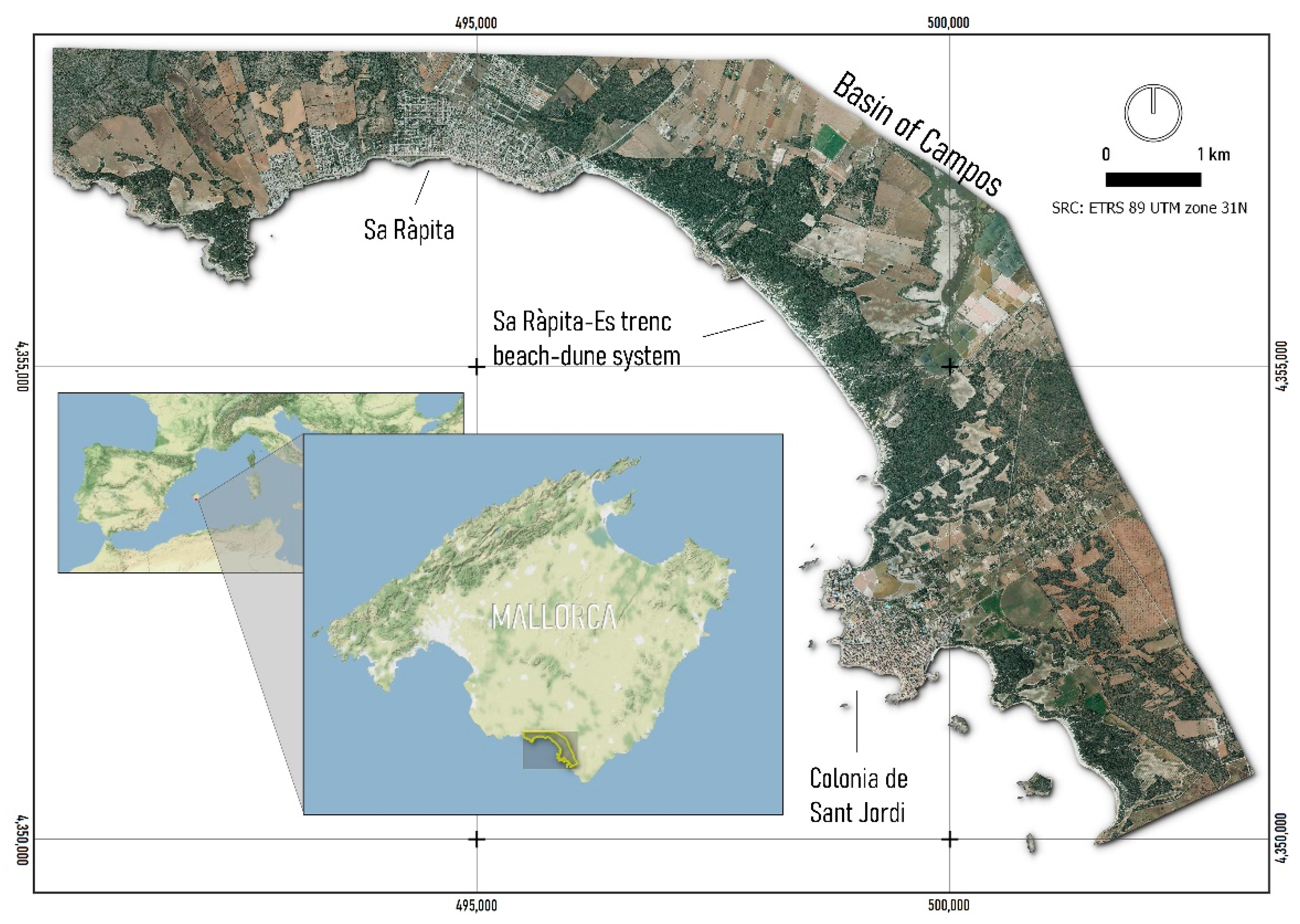
2.1. Study Area

The beach-dune system of Sa Ràpita-es Trenc is located on the Southern coast of the island of Mallorca (Western Mediterranean), on a coastline that closes the basin of Campos to the sea (Figure 1). The system has an approximate area of 9 km2 occupied by Holocene dunes. These dunes extend along an arched coastline of about 6 km that goes from the town of Colonia de Sant Jordi to the marina of Sa Ràpita, in a westerly direction. The construction of the marina in 1973 caused a retreat of the coastline in the central sector [52]. The rocky promontories that emerge between the dune systems and on which the town of Sant Jordi is located are formed by eolianites. The rocky coast of strata beyond the marina in a westerly direction is formed by the outcrop of post-orogenic upper Miocene materials (calcarenites). The composition of the beach sand is predominantly bioclastic with a fine texture [53]. The presence of the seagrass Posidonia oceanica in the submerged beach is a key factor in fixing and stabilizing the sediment in the nearshore area, and their dead leaves deposited as banquette in the aerial beach protect it from erosion during storms. A study about the evolution of the coastline of the beach between 1956 and 2015 showed a total average regression of −5.72 m [54].
The reasons for choosing this study area (30.92 km2) are related to its remarkable geomorphological dynamism (many potential changes occurred in the shorelines, beaches, and dunes during the studied period) and the limited altitudinal gradient. In addition, the presence of the sea limited some steps of the workflow (i.e., the capture of Ground Control Points). These three features challenged the implementation of the SfM-MVS methodology, making this pilot area an ideal site for testing the proposed workflow [38,40,55].

2.2. Dataset

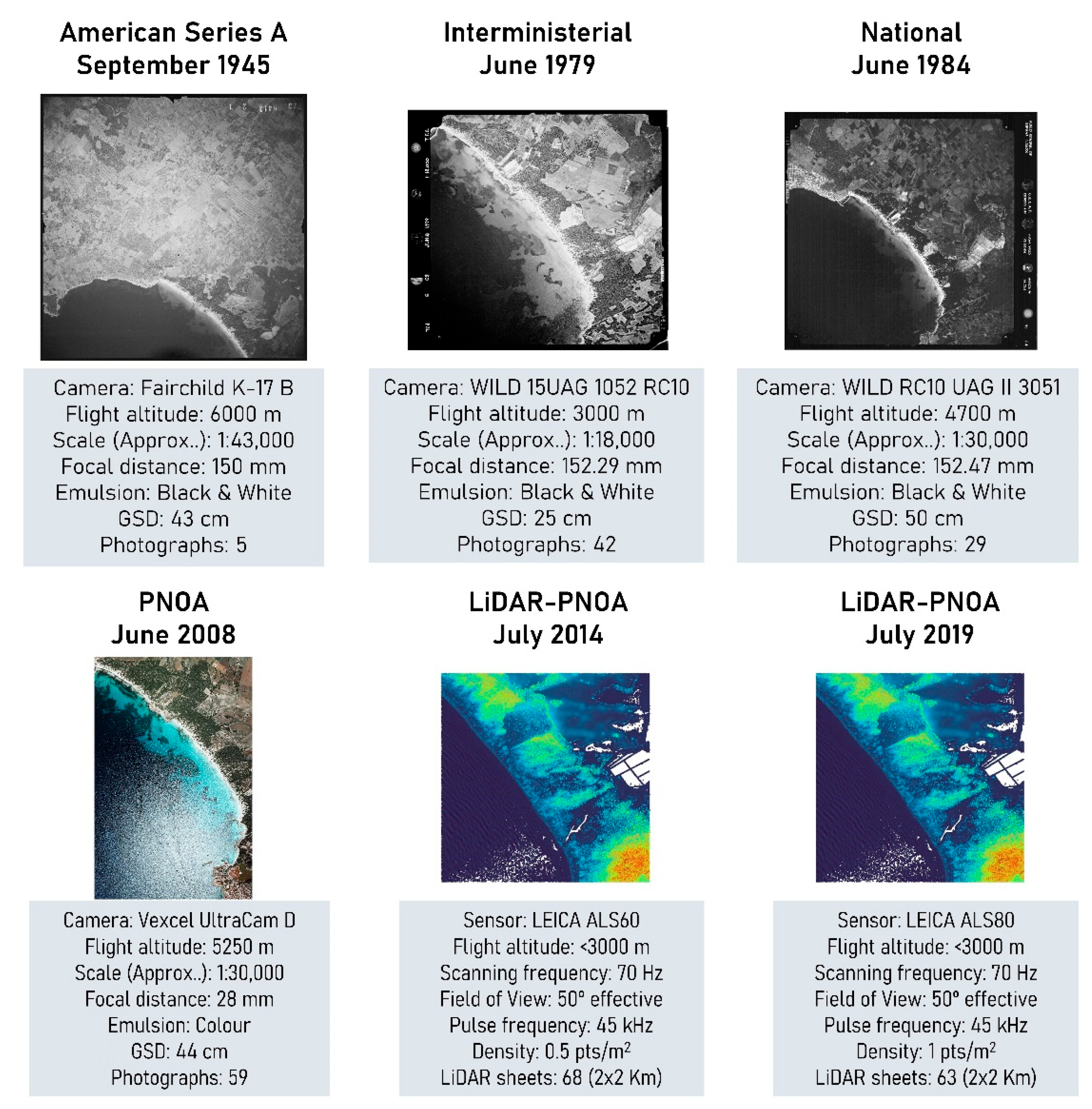
2.2.1. Historical Aerial Image Series

A total of four sets of historical aerial photographs covering a 30.92 km2 study area were processed using SfM-MVS methods. Image datasets correspond to aerial surveys carried out in 1945 (American A Series), 1979 (Interministerial Flight), 1984 (National Flight), and 2008 (Spanish PNOA Flight) (Figure 2) [56]. The Centro Nacional de Información Geográfica (CNIG) (https://centrodedescargas.cnig.es/ (accessed on 1 April 2022)) provided historical photographs from 1979 to 2008. Photographs corresponding to the 1945 survey were obtained from the U.S. National Archives and Records Administration (NARA) (https://www.archives.gov/ accessed on 1 April 2022 (available upon request)).
The different sets of photographs were taken with different cameras during the summer, at different morning hours with different solar elevation angles and from different altitudes, ranging from 6000 to 3000 m above sea level, so the scales of each series of photographs differ. All historical image sets, except the 2008 PNOA photo series, have a fiduciary system defining the flight metadata, reference system, and scales. The black and white photographs from 1945 to 1984 were captured with very little frontal and lateral overlap, particularly in the 1945 series, where only seven photographs were captured in two strips parallel to the shoreline. These images were scanned from analog to digital and used without a reference system. All the black and white photographs used in this study present challenges for photogrammetric processing due to the noise in the photographs, the presence of the sea in some photographs, and photogrammetric quality issues such as overlap, scale, and uneven distribution of GCPs on the shoreline. The RGB photographs captured by PNOA 2008 have higher photogrammetric quality in terms of image definition, contrast, and overlapping, and they are adequate for an SfM-MVS experiment.
More flights and historical photographs are available for public use and download at CNIG and the Digital Fototeca of Spain (from 1929 to 2022) (https://fototeca.cnig.es/fototeca/ (accessed on 1 April 2023), though their use for SfM-MVS in this study was discarded due to insufficient overlap (i.e., the 1956 American B series and the 1991 coastal flight series) [49]. Still, we aimed to obtain a coherent and reliable DSM with just five photographs (1945 American Series A) (Figure 2 and Figure S1).

2.2.2. LiDAR ALS

In order to validate the hDSM series obtained using SfM-MVS, we used official products derived from ALS (Airborne Laser Scanning). In this case, ALS datasets from 2014 and 2019 belonging to flights of the Spanish National Aerial Orthophotography Plan (PNOA) have been processed. These files have also been downloaded from the Spanish National Centre for Geographic Information (CNIG) (https://centrodedescargas.cnig.es/ (accessed on 1 April 2022).
The 2014 and 2019 datasets present very similar characteristics, such as flight altitude, scanning or pulse frequency, field of view, as well as other attributes, although some differences are also observed. The main differences between the datasets analyzed are the sensors—the LEICA ALS60 for 2014 and the LEICA ALS90 for 2019—but the most notable and important difference is the laser spot density. In the 2014 dataset, the density is 0.5 points per m2, whereas in the 2019 dataset, a higher density is observed, reaching 1 point per m2.

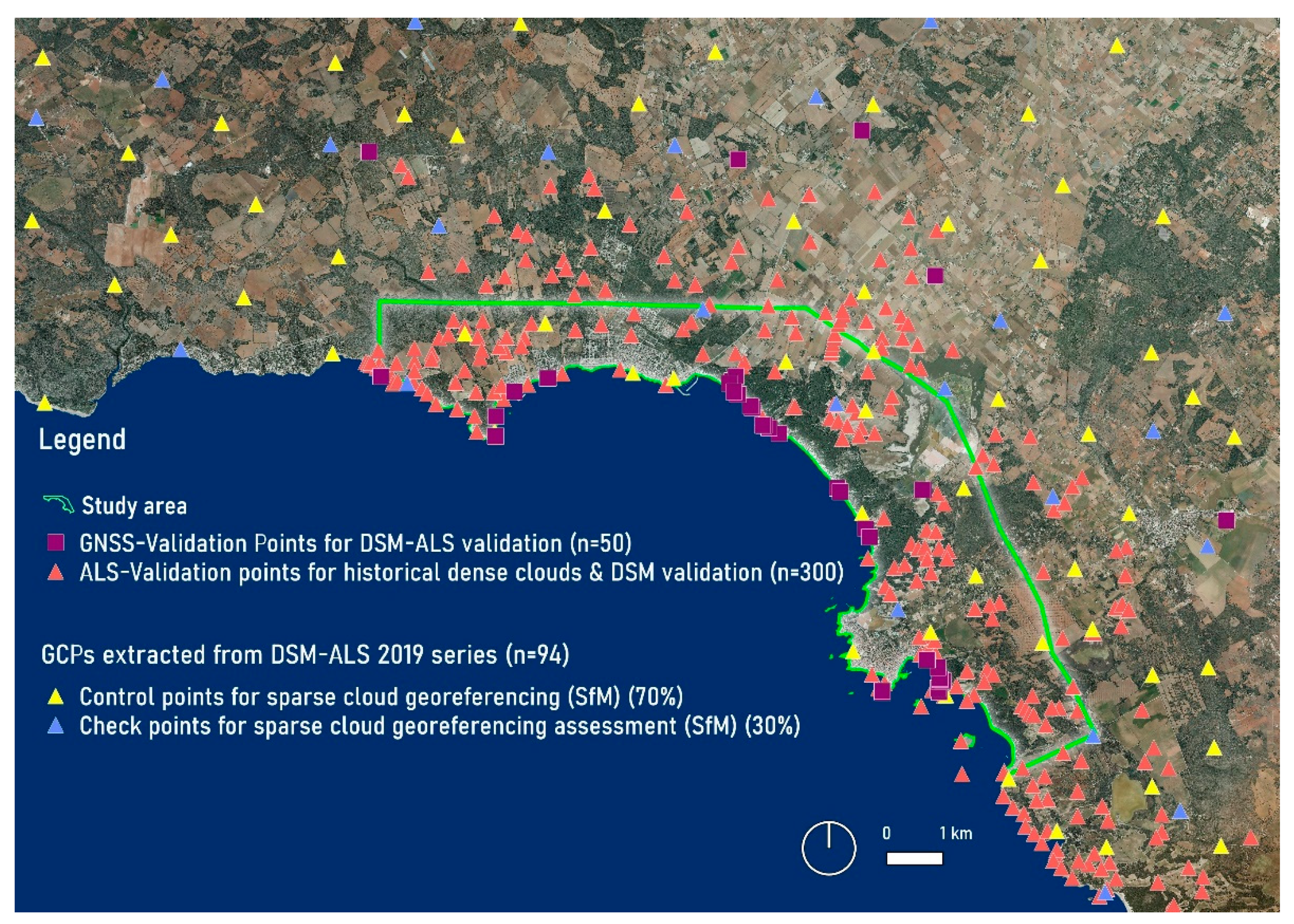
2.3. GNSS: Reference Field Survey

On 11 December 2021, a total of 50 GNSS-validation points distributed over the ALS cloud area (Figure 3) were measured using a Leica Viva GS15 GNSS system (Leica Geosystem AG, Heerburg, Switzerland). This receiver is outfitted with a real-time kinematic transmission (RTK) positioning system with a differential connection to the SITIBSA XGAIB service (Servei d’Informació Territorial de les Illes Balears and Xarxa de Geodèsia Activa de les Illes Balears). These reference GNSS-validation points were utilized for independent positioning validation of the DSM-ALS (2014 and 2019). The equipment specified for RTK accuracy in static phase mode is 5 mm horizontal plus 0.5 ppm RMSE and 10 mm vertical plus 0.5 ppm RMSE. The coordinates were first recorded in the WGS84 ellipsoid reference (epsg:4326) and subsequently translated to the ETRS89 UTM zone 31N coordinate reference system (epsg:25831). GNSS-validation points were measured at areas with minimal vertical change [56] between the 2019 DSM-ALS series and the GNSS survey (2021), such as bunkers, flat rocky surfaces near the coast, and inland road crossings.

2.4. Ground Control Points

GCPs were edited using QGIS software [57] by selecting sites where elevation changes in the historical dataset were limited, such as anthropogenic features [4,5]. We avoided identifying GCPs in the beach-dune system due to its high morphodynamical activity. Vertical coordinates (z) of GCPs were retrieved using the ALS 2019-derived DSM, while horizontal coordinates (xy) were extracted from the PNOA 2019 orthophotography.
We used 94 GCPs, uniformly distributed over the photogrammetric area (Figure 3), and randomly grouped into Control Points to georeference the sparse cloud and Check Points to assess the xyz accuracy of the sparse cloud in the SfM process. An additional and independent sample of 300 GCPs was employed as ALS-Validation Points for historical dense clouds and DSM evaluations as final deliverables.

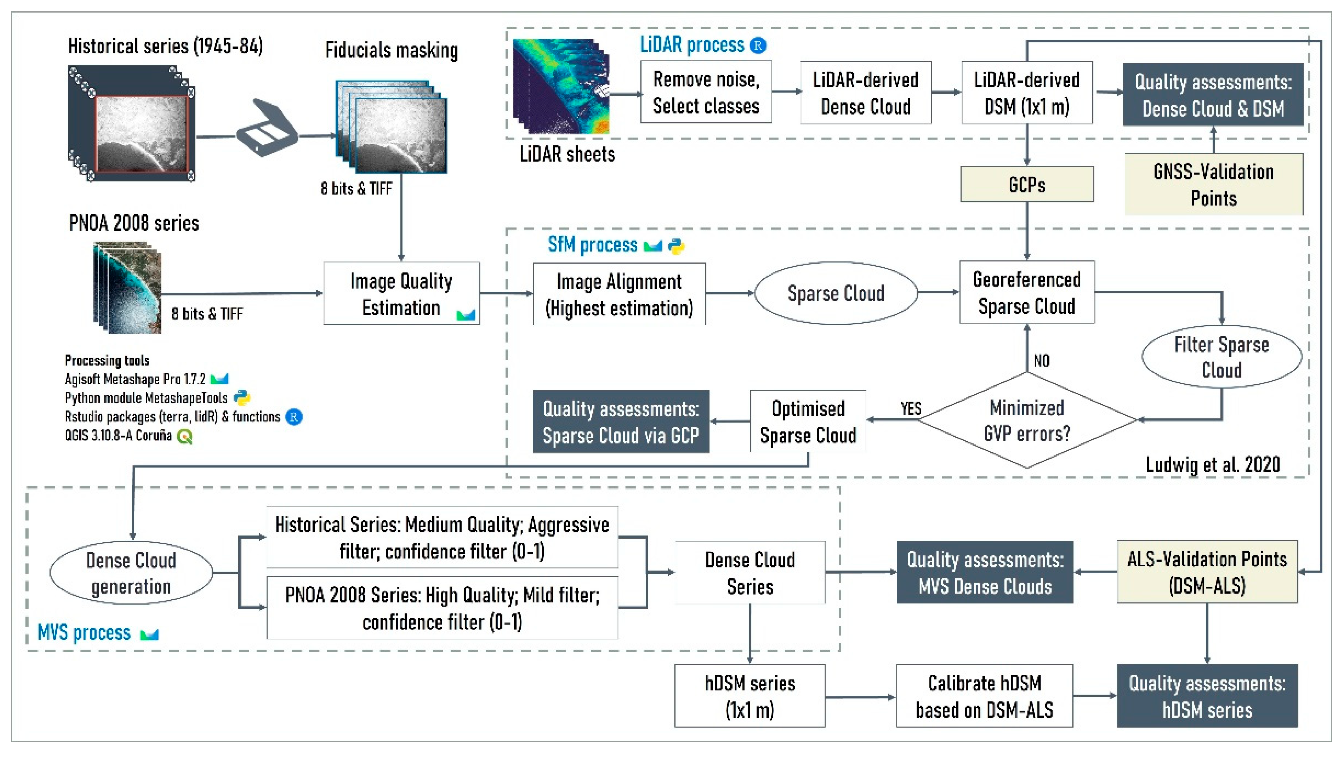
2.5. LiDAR ALS and Historical Aerial Photographs Processing

The effective and complementary use of LiDAR datasets for validation of SfM-MVS-derived hDSM series has already been tested [38,39,40,58,59], highlighting the usefulness of ALS-derived DSMs to work as ground truth for elevation value comparisons in large or inaccessible areas where the use of punctual GNSS data for the validation is not an option. Thus, in this study, using GNSS measurements, we first assessed the quality of two ALS coverages that subsequently were used as ALS-Validation Points to validate the historical DSM series.

2.5.1. ALS Processing for DSM Generation

The LAScatalog tool implemented in the open-source package lidR (version 4.0.2) of R statistical software [25] was used to process ALS data to generate DSMs. The LAScatalog processing engine’s functionality allowed us to apply a processing routine in the area of interest without having to load the ALS cloud collection into CPU memory, allowing us to process high-density datasets quickly. The processing included the fusion of ~234 million spatialized points into 68 ALS sheets and ~341 million into 63 ALS sheets for the 2014 and 2019 series, respectively, as well as noise removal and the extraction of seven coverage classes for both series over the recognized surfaces in the study area (bare ground, low, medium, and high vegetation, buildings, water, and surfaces reserved by the American Society of Photogrammetry and Remote Sensing, ASPRS).
Then, we generated DSM series derived from the classified ALS clouds using the Inverse Distance Weighting (IDW) interpolation method on 1 m × 1 m grids and saved them in TIFF format in the ETRS89 UTM zone 31 coordinate system.

2.5.2. Historical Aerial Photograms SfM & MVS Processing DSM

The SfM-MVS method was used to generate point clouds and based upon them, DSM and orthomosaics series from a set of historical aerial photographs taken in 1945, 1979, 1984, and 2008. The SfM-MVS process was carried out using the commercial software Agisoft Metashape Professional [60] version 1.7.2 build 9097, 64-bit, and a Python module for MetashapeTools (https://github.com/envima/MetashapeTools/ accessed on 1 April 2022) provided by [61].

SfM Process to Generate Optimized Sparse Cloud

Prior to SfM startup, the sets of photographs were ingested, the fiducial marks on the edges of the photographs were masked, the xyz coordinates represented by the centroids of each photograph were imported, and the image quality (IQ, range 0–1) of each photograph was estimated based on the degree of sharpness. As a result, no photograph had an IQ estimate lower than 0.84, so it was unnecessary to eliminate photographs since Metashape specifications recommend using only photographs with an IQ greater than 0.5.
The SfM process started with the estimation of the raw sparse clouds produced by image alignment, which included specific Metashape algorithms for aerial triangulation (AT) and block bundle adjustments (BBA). To find tie points in multiple overlapping and randomly acquired photographs, both algorithms rely on feature extraction and feature matching. Image alignment was set to “high” for the 1945 series, “medium” for the 1979 and 1984 series, and “highest” for the 2008 series in order to obtain accurate estimates of camera position for each photograph in each series. As a result, we obtained sparse clouds projected in photogrammetric coordinates that lacked the actual scale, orientation, and position.
The sparse clouds were georeferenced into the same coordinate systems as the corresponding image set, WGS84 (1945 series) and ETRS89 UTM zone 31 (1979, 1984, and 2008 series), by interactively marking the GCPs on the photographs (Section 2.4). Due to the low accuracy of the photographs’ telemetry data, we first deactivated it during the process. The GCPs were then interactively placed on at least two to three photographs of the 1945 series, three to four photographs of the 1979 and 2008 series, and four to five photographs of the 1984 series. The sparse clouds were linearly transformed using the transform update tool, with a similarity transformation of 3 for translation and 1 for rotation. In this process, we randomly grouped 70% of GCPs into the Control Points sample and 30% of GCPs into the Check Points sample to validate the geolocation accuracy of the sparse clouds.
Estimation of camera orientation is frequently inhibited in SfM due to the low accuracy and spatial distribution of tie points, resulting in nonlinear deformation in the georeferenced sparse cloud [62]. Tie points can be arbitrarily removed to resolve this effect, but doing so risks affecting the quality of the 3D transformation process. In this study, as an alternative, we used an iterative optimization method to improve sparse cloud accuracy by removing points that exceeded a certain error and reoptimizing the camera position [61]. The process starts with conservative filtering of the quality attributes of the sparse cloud (see [60] for a detailed description of the quality attributes of the sparse cloud), with the maximum values of the reprojection error (RE), reconstruction uncertainty (RU), and projection accuracy (PA) thresholds set to 1, 50, and 10, respectively. The next step is the iterative optimization of camera parameters and camera positions. The process ends with a dynamic search for the RE threshold value, using tie points from the filtered sparse cloud that have minimal reprojection errors as the unique candidates. As a result, the RMSE between the observed coordinates of the Check Points and the estimated point of the sparse cloud is minimized.
In SfM, we created the orthomosaics series based on 2.5D meshes interpolated by the points of the optimized sparse clouds using the Triangulation Irregular Network (TIN). The orthomosaics were saved as TIFF format images in 1 m × 1 m grids in the ETRS89 UTM zone 31 coordinate system.

MVS Process to Generate Dense Point Clouds and DSM

Using the MVS method, we produced dense clouds from optimized sparse clouds. Since the “image quality” parameters and the “depth map” filters in the Metashape software determine how well dense cloud reconstructions turn out, we selected 3D reconstruction settings to reduce geometric errors in each series. Thus, for the 1945 and 1984 series and for the 1979 and 2008 series, we used the image quality levels “medium” and “high,” respectively. Given the high noise presented by the black and white image series, we kept the depth filtering level at “aggressive” to minimize the estimation of suspect points. We opted to keep the “mild” depth filtering level for the 2008 RGB series due to better photogrammetric quality. Due to excessive noise production at the “ultrahigh” image level, it was decided to exclude it from the analysis. Additionally, we estimated confidence thresholds at each point in the dense clouds and removed those with the lowest levels of confidence (0–1 within a range of 0–255).
In order to create an hDSM series, the dense cloud series were rasterized in Metashape using the IDW interpolation method on 1 m × 1 m grids. The DSMs were then saved in TIFF format in the ETRS89 UTM zone 31 coordinate system.

2.6. Quality Assessments

2.6.1. ALS-Derived DSM

We evaluated the accuracy of the DSMs derived from the official ALS cloud products using high-precision GNSS-Validation Points obtained from GNSS readings (see Section 2.3). To do so, we computed linear regressions, comparing the observed GNSS-Validation Points to those predicted by the 2014 and 2019 DSM based on ALS, and we assigned these products a measurement quality score using the coefficient of determination R2 and MAE (Mean Absolute Error). MAE is a widely used metric for (regression) model evaluation in geosciences [63] and is defined as the average absolute difference between the predicted and observed values.

2.6.2. Aerial-Photographs

Optimized Sparse Cloud in SfM

To assess the measurement accuracy of the optimized sparse clouds of the historical photogrammetric series, the reprojection root mean square error (RMS RE) and check points RMSE estimates were used. The RE sparse cloud attribute was estimated by measuring the distance in pixels between the projected image point at a reconstructed 3D point and the original projection of that 3D point detected in the images. This metric serves as the foundation for the sparse cloud reconstruction procedure. The Euclidean distance between the check point coordinates depicted by DSM-ALS and those predicted during the iterative process of georeferencing the sparse cloud was used to calculate the check point RMSE. We compared the optimized sparse clouds to the raw clouds to assess the effect of the optimization method on SfM using RMS RE and check point RMSE.

Global Quality Assessment and Calibration of SfM-MVS DSMs

We calculated linear regressions between the observed ALS-Validation Point values (see Section 2.4) derived from the best DSM-ALS (2019) accuracy assessment (see Section 2.6.1) and the values predicted by the photogrammetric DSMs to assess their accuracy. The Leave One Out Cross-Validation (LOOCV) approach (caret R-package) was used to improve the elevation accuracy and produce a series of historical DSMs adjusted to the elevation values of the official DSM-ALS 2019 series. This method was based on calculating the different positions of the slope and intersection coefficients (x = y) between the photogrammetric DSMs and DSM-ALS 2019 and then applying these coefficients to the full resolution of the photogrammetric DSMs to calibrate them. To provide precision quality values to the resulting photogrammetric DSMs, we use the coefficient of determination (R2) and Mean Absolute Error (MAE).

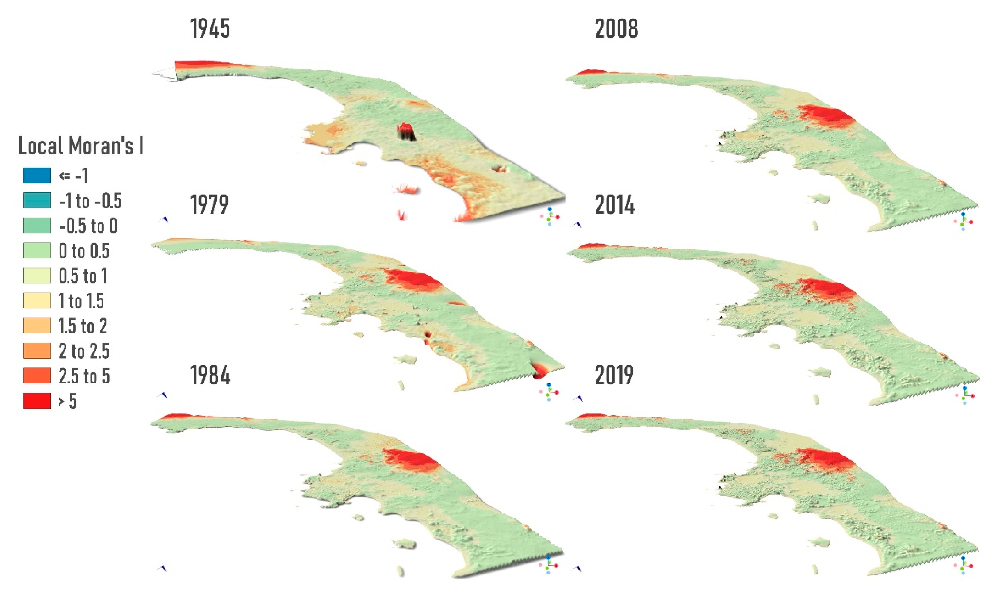
2.6.3. Local Quality Assessment of DSMs Series

Although MAE and R2 provide an overall quality value for the resulting DSMs, it may not be informative of the spatial distribution of the DSM error; elevation models, by definition, have spatial behavior, as does their error. This means that systematic, random, or coarse elevation errors are frequently spatially autocorrelated [62]. Hence, we quantified the Local Moran Index (raster R-package) to map, identify, and evaluate elevation errors or patterns at the local level.
All the procedures and calculations (Figure 4) were run on a standard desktop computer equipped with an Intel (R) Core (TM) i7-8700 CPU @ 3.20GHz processor and 32 GB of RAM.

3. Results

3.1. ALS-Derived DSM

Raw ALS data used in this study was composed of two sets of point cloud sheets (2014 and 2019 coverages) of 2 × 2 km, encompassing the pilot study area described in Section 2.1. These were used to obtain two ALS-derived DSMs at 1 m spatial resolution (pixel size), following the procedure described in Section 2.5.1. Validation of ALS-derived DSMs was made by comparing point z values with GNSS-Validation Points. We found a very strong (R² > 0.99) agreement between GNSS data and both DSMs (2014 and 2019), highlighting the reliability of both coverages of Spanish PNOA ALS data after the application of a very rudimentary quality control procedure (error/noise removal protocol) (Section 2.5.1).
PNOA official metadata for Spanish ALS coverages estimates the overall elevation RMSE of the Balearic archipelago’s point clouds at 0.2 and 0.15 m, respectively, for the 2014 and 2019 flight campaigns (https://pnoa.ign.es/web/portal/pnoa-lidar/ (accessed on 1 July 2022). These figures are similar to those obtained for our study area, shown in Table 1. The 2019 ALS-derived DSM outperformed in terms of elevation accuracy (z error), due to its greater point density (341 million points, 1 point/m²), compared to 2014 ALS point cloud characteristics (234 million points, 0.5 points/m²). Thus, the uncertainties and errors inherent to the interpolation (IDW) process to derive the DSM are of lesser importance in the case of the 2019 ALS coverage, since for each pixel of the DSM (the objective is to obtain a DSM of 1 m pixel size), there is a corresponding point cloud elevation value to include in the calculations. This feature makes the 2019 ALS-derived DSM error rate drop compared to the 2014 ALS; therefore, the former was considered our ALS-Validation Points for comparison purposes and for assessment of the quality and accuracy of the SfM-derived hDSM series.

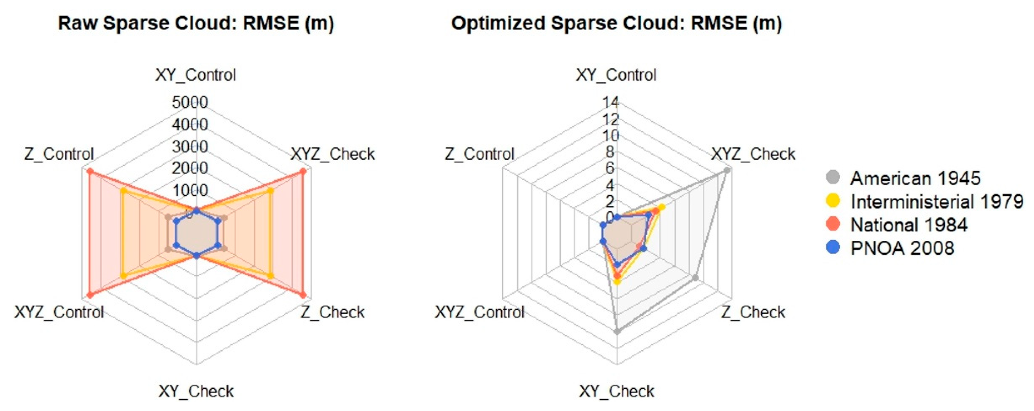
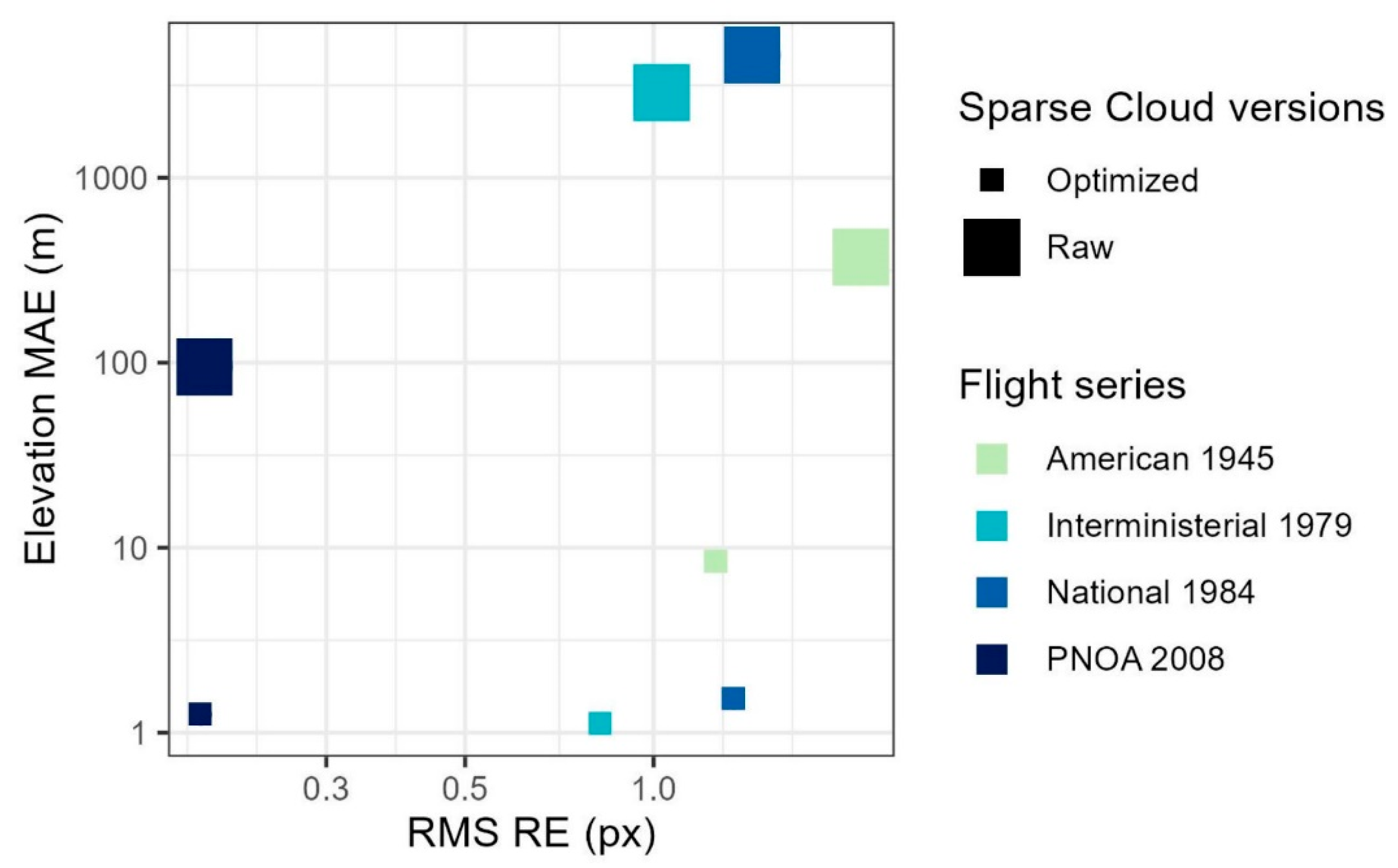
3.2. Optimized Sparse Cloud in SfM

Prior to calculating the hDSM series from SfM-MVS, four different sets of historical aerial photographs (1945, 1979, 1984, and 2008 survey flights) were used to generate the corresponding sparse clouds in SfM (see Section 2.5.2). The image alignment procedure estimated raw sparse clouds from tie points of 13,700 (1945), 157,548 (1979), 78,351 (1984), and 85,207 (2008), with RMS RE ranging from 2.148 px for the 1945 series to 0.192 px for the 2008 series (Table 2). The MAE of these sparse raw clouds compared with check points was 372.7 m (1945), 2856.5 m (1979), 4595.5 m (1984), and 95.3 m (2008) in elevation (z) values.
The sparse cloud optimization process produced optimal RE thresholds of 0.24 (1945), 0.13 (1979), 0.25 (1984), and 0.10 (2008), which removed 31.01% (1945), 8.8% (1979), 7.08% (1984), and 0.54% (2008) of suspect tie points and improved the RMS RE for all series, though the reduction was greater (about 1 px) in the case of the optimized 1945 sparse clouds (Table 2). The importance of this step is also demonstrated in Figure 5, where significant elevation errors (check points RMSE) recorded in the raw sparse clouds are drastically reduced (two and three orders of magnitude, depending on the flight considered) in the optimized sparse clouds. This occurred as expected, especially when considering the control point RMSE, which was very close to 0 in all cases. When check point errors are considered, the improvement is also significant (RMSE 1.6 m in the 1979, 1984, and 2008 optimized sparse clouds). The 1945 optimized sparse cloud is an exception, as it still has a check point RMSE in z of around 10 m.
The most significant improvements in modelled elevation values were observed for the 1979 and 1984 coverages: correlations with check points skyrocketed (R² ≈ 0.3 to R² > 0.99) and elevation errors decreased greatly (MAE > 2800 m to MAE ≤ 1.52 m). The raw 2008 sparse cloud had the highest accuracy among the non-optimized clouds, so its improvement after optimization was modest. Nevertheless, when compared to the raw cloud, the optimized 2008 sparse cloud reduced the elevation MAE by more than 94 m. The results for the 1945 optimized sparse cloud are unsatisfactory: correlations with check points improved but appear insufficient (R2 = 0.58). The same can be said about the MAE elevation (from 372 m to 8.47 m). The low accuracy of the 1945 sparse clouds is understandable, given the small number of photographs (5) and overlap (summarized by the quality attribute Image Count (IC) of the tie points) between them (see Figure S1) available in the 1945 data set (see Figure 2). In summary, an increase in elevation accuracy in terms of MAE and an improvement in RMS RE in Figure 6 demonstrate the critical importance of the sparse cloud optimization stage for this study.

3.3. Calibrated DSMs Derived from Aerial Photography

We generated MVS dense clouds for each series in Metashape by combining the “medium” (1945–1984 series) and “high” (2008 series) image quality options with the “Aggressive” and “Mild” filtering options, respectively. The computational load increased significantly, as expected, from ~8 m for the 1945 black and white series to ~10 h for the 2008 RGB series. Likewise, the density of cloud points increased from 9 × 10⁶ to 359 × 106. Filtering points with confidence values between 0–1 reduced dense clouds by 6.81% (1945), 19.03% (1979), 12.78% (1984), and 11.92% (2008), resulting in MAE elevation values of 8.22 m (1945), 1.74 m (1979), 1.58 m (1984), and 0.91 m (2008) compared to ALS-Validation Points (Table S1).
After the interpolation (IDW) of dense clouds z values for DSM series rasterization, DSM elevation values underwent a calibration process (see Section 2.6.2), being adjusted to the ALS-Validation Points. This procedure contributed to another substantial improvement of the proposed workflow by reducing elevation errors in three of the four photography datasets (Table 3): from 7.75 m to 5.21 m (1945 DSM), from 0.87 m to 0.71 m (1984 DSM), and from 0.43 m to 0.41 m (2008 DSM). Unexpectedly, elevation MAE of the 1979 DSM increased after calibration by 0.53 m. This issue will be the subject of further reflection and comments in the discussion section.

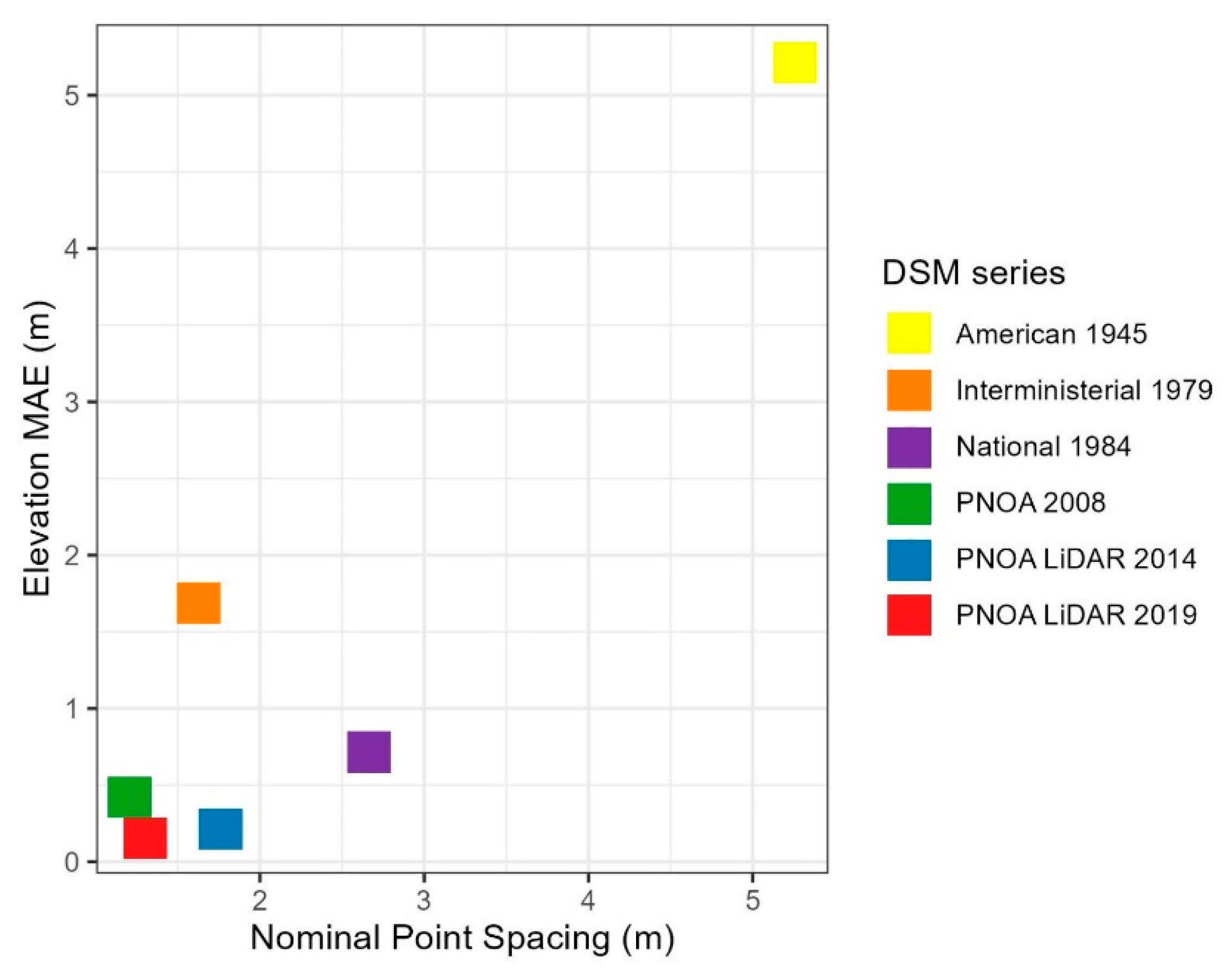
3.4. Quality Assessments of the DSM Series

The results of the quality assessment of the generated hDSM series are shown in Table 4. The four most recent datasets, including historical photographs and ALS as source information (1984, 2008, 2014, and 2019), exhibit quite acceptable quality features, making them a reliable source of spatially distributed elevation information. In these four cases, correlations between the hDSM and its respective ALS-Validation Points are very high (R2 > 0.98), and the MAE in z remains below 0.71 m in all cases. All this means that the proposed workflow is capable of obtaining accurate and high quality hDSM series over a time span of almost 40 years (1984–2019) and with a wide range of applications. The 1979 DSM also presents good quality features and accuracy (R2 = 0.89 against validation and MAE below 1.7 m), which also makes it a fairly reliable dataset for certain tasks and applications. As expected, (see Section 2.2), the worst performance of the quality assessment was obtained by the 1945 dataset, showing moderate correlation (R2 = 0.5) with the ALS-Validation Points and an elevation MAE above 5 m.
Spatial global autocorrelation statistics (i.e., Global Moran’s I and Global Geary’s C) show values near to perfect correlation (Moran’s I positive and close to 1, Geary’s C close to 0) for the four most recent datasets (1984, 2008, 2014, and 2019) (Table 4), meaning that these hDSM (and ALS-derived DSM) are spatially coherent and free of artifacts and systematic (or random) errors. The great performance of the 2008 DSM is noteworthy, which features the best global autocorrelation statistics among all considered DSMs and also has the greatest gridded point cloud density (0.686 pts/m2, even higher than those corresponding to the 2019 and 2014 ALS-derived DSMs).
Local autocorrelation maps for the six generated DSMs (Figure 7) show the degree to which one areal unit is autocorrelated relative to its neighbors. The analysis clustered DSM elevation values according to the resemblance of each pixel to its neighbors, grouping pixels in three main categories observed in the six DSMs: i) Moran’s I ≥ 0.5 and ≤ 1.5 (ochre color in Figure 7 maps), very low (even below sea level) and flat areas with very small topographic variations corresponding to crop fields and salt lakes; ii) Moran’s I ≥ −0.5 and ≤ 0.5 (green color in Figure 7 maps), areas with gentle slopes covered by natural vegetation (pinus halepensis forests); iii) Moran’s ≥ 2.5 (red color), steeper slopes covered by natural vegetation (pinus halepensis and shrubs) or urban land use. Moran’s I values between 1.5 and 2.5 (orange color in Figure 7), only recorded in the 1945 and 1979 DSMs, correspond to artifacts and deformities caused by the insufficient quality of the photographs involved since they are only present in these two datasets and do not correspond to actual changes that occurred in the topography of the study area in recent decades.
As well as the aforementioned errors, more evident artifacts and outliers can be observed in the depiction of Local Moran’s in the 1945 and 1979 DSMs: (i) the insufficient overlapping and coverage of the 1945 photograph dataset directly caused the impossibility of generating the 1945 DSM in the westernmost sector of the study area (a line cutting the DSM can be observed in Figure 7); (ii) in two olive crop fields, an anomalous butte-shaped “topography” appears in the middle of the 1945 DSM (see Figure S2); and (iii) sinks and crater-shaped artifacts can be randomly found across both the 1945 and 1979 DSMs. Nevertheless, the four remaining DSMs (1984, 2008, 2014, and 2019) look free of anomalies, artifacts, or deformities, as corroborated by the spatial autocorrelation analysis.
The overall picture of DSM series quality, combining an accuracy metric with a point density metric, is summarized in Figure 8. Two relationships between the nominal point spacing (density metric) and elevation (z) MAE (accuracy metric) can be observed: (i) for the four most recent image datasets (1984, 2008, 2014, and 2019), the ratio of increase in elevation error with respect to point spacing is roughly 1 to 3 (for each 3 m of point spacing increase, elevation error grows by 1 m); (ii) for the two oldest datasets (1945 and 1979), the ratio is 1 to 1, highlighting the use limitations of the two oldest datasets. In the case of the 1945 DSM, it is clear that the handicap of having only five photographs available resulted in a very low point density (nominal point spacing > 5 m) that sharply decreases the accuracy (see Figure S1). Altogether, this means that an increase greater than 3 m in point spacing has critical consequences for the DSMs’ accuracy level and, therefore, the DSM is unable to retain small topographic variations, as occurred with the 1945 DSM.

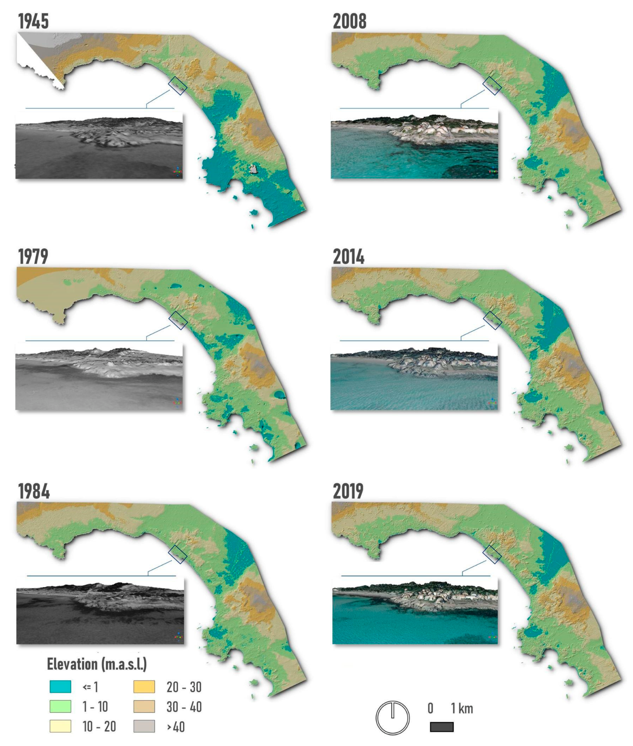
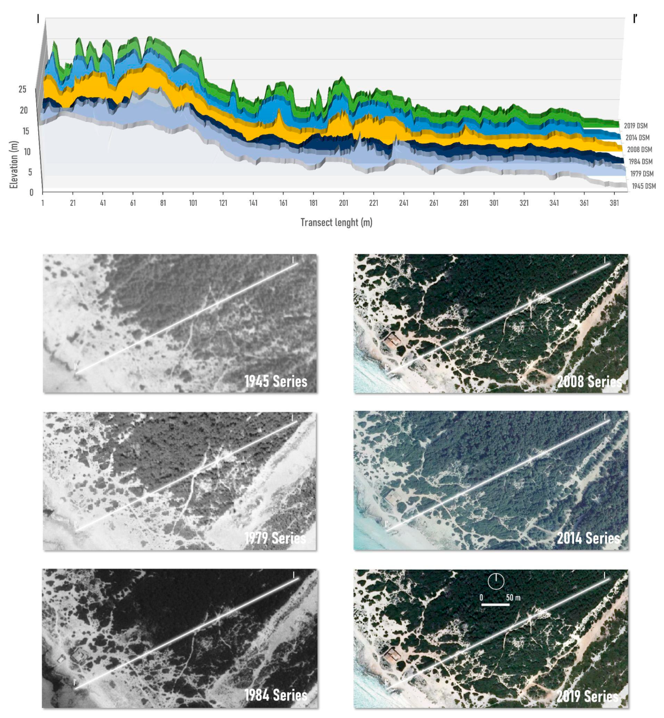
3.5. Historical DSM Series Showcase

The final products of the proposed workflow (i.e., the optimized and calibrated historical DSM series) are shown in Figure 9. As expected, DSM generated with the most recent datasets (1984 and 2008 historical image sets and 2014 and 2019 ALS coverages) show very good agreement, recognizable and coherent patterns, and look artifact-free in an overall view. On the contrary, evident errors and artifacts can be observed in the 1945 and 1979 DSMs. In addition to not being able to generate the 1945 DSM in the westernmost sector, elevation estimation by the model in this area is also poor, featuring coarse errors and abrupt topographic changes that are not real as a consequence of the insufficient overlapping between images in these areas (Figure S1). In the Southern end of the 1945 DSM, an “artificially created” sinking of the topography is clearly observable in a number of areas with false topographies below 1 m.a.s.l. We hypothesize that this is another consequence of the scarce number of images involved in the calculations of the sparse clouds in these areas or issues with image texture/contrast difficulty in the calculation of the tie point during the sparse cloud generation. Moreover, the errors appearing randomly across the study area and detected by the autocorrelation analysis in the previous section are seen in the 1945 and 1979 DSMs as areal (1945) and punctual sinks (1979) (dark green color in Figure 9).
For illustrative purposes, Figure 10 shows an elevation transect comparison among the six DSMs, corresponding to a representative sector of the beach-dune system (covering the emerged beach, the foredune, and the dunes) that underwent several changes between 1945 and 2019. Among these changes, an evident process of revegetation and densification is observable throughout the sequence of orthomosaics, especially after the tree removal process captured in the right part of the photographs, created by flooding between 1945 and 1979.
The ‘artificially smoothed’ topography generated by the coarse point density of the 1945 DSM (nominal point spacing > 5 m) is clearly observable in the (gray) profile graph, and although this DSM manages to retain the overall variability of the transect, it fails to reproduce fine-scale changes and details (canopy cover and microtopography). The 1979 DSM is also able to retain the large-scale topographic pattern, although it presents constant underestimations of elevation values across the transect, probably caused by the artifacts detected by the spatial autocorrelation analysis previously described (Figure 7). The same is applicable to the 1984 DSM transect, although underestimations were observed for canopy (pine forest) elevations (60–100 m transect lengths). This issue could be related to the dark coloring (low brightness and contrast) of images in the 1984 data set, which appear almost black in the pine forest area: in these areas, the limits of the tops of the trees are indistinguishable, and the software has difficulties calculating elevation references (tie points). Transect graphs corresponding to the 2008, 2014, and 2019 DSMs show great agreement among them, with the most notable differences observed in vegetated sectors, where the growth and densification of vegetation that occurred between 2008 and 2019 can be identified.

4. Discussion

In this study, we proposed, tested, and quality assessed an optimized SfM-MVS workflow for the generation of DSMs using historical photograph series (1945, 1979, 1984, and 2008) and two ALS coverages (2014 and 2019). The objectives were (i) to obtain high resolution (1 m pixel size) and high-quality hDSM series based on these photographs, minimizing errors present in the original data sets (i.e., georeferencing and reprojection) or generated during the implementation of the workflow (elevation calibration); and (ii) to evaluate those errors in order to assess the quality of the obtained products (hDSM series). We aimed for optimization in terms of the accuracy of the product generated and also in terms of saving computer processing time. The design of the workflow (see Figure 4) was intended to be reproducible and applicable in other spatial settings [64]. The numerous potential uses and applications of the hDSM series have increased interest in SfM-MVS methodologies in recent years, and many examples of SfM-MVS workflows used for historical hDSM generation can be found in the literature [38,40,42,65]. Nevertheless, photogrammetric use of the Spanish historical photograph archive has been scarce to date [49].
The reasons for choosing this study area are also related to its remarkable geomorphological dynamism (many potential changes occurred in the shorelines, beaches, and dunes during the studied period [52]) and the limited altitudinal gradient. The coastal fringe also introduced limitations for GCP’s capture and made this task impossible over the sea (which covers a significant portion of many photographs). These three features, together with the characteristics of the set of historical photographs, challenged the implementation of the SfM-MVS methodology and conditioned the quality of the photogrammetric hDSMs [66]. The testing of the optimized workflow in this pilot area allowed us to unveil errors and artifacts eventually associated with low-elevation areas (and of limited elevation gradient), many of them below sea level. This low elevation gradient together with the presence of the sea affected the generation and quality of the 1945 and 1979 DSMs, limiting GCP’s capture and the recognition of tie points.”

4.1. ALS-Derived DSM

The LAScatalog processing engine [25] has been demonstrated in this study to be a very useful tool for designing processing routines for large LiDAR sheet sets for a complete ALS cloud acquisition, without the need to load them onto the CPU. Furthermore, with only a few short lines of open-source code based on R statistical software, the LAScatalog framework allows the generation of automated workflows for DSM generation, which are thus reproducible for different time series or applications in other environments [64]. All these factors, combined with the availability and trustworthiness of official and ASPRS standardized ALS cloud data (in our case, the 2014 and 2019 ALS PNOA coverages), provided us with the opportunity to develop a workflow based on the fusion of millions of points, error/noise removal, coverage extraction, and IDW interpolation of points for the generation of very high accuracy DSMs. However, the lower ALS point density of the 2014 coverage resulted in lower MAE elevation accuracy than that of 2019. As a result, the lower the density, the lower the accuracy of the reconstructed model, resulting in higher uncertainty and errors inherent in the interpolation process (IDW) to derive a DSM in lower density areas. If accuracy in terms of MAE and density metrics are both expressed as DSM quality criteria, the ALS 2019 will be considered valid as a reference product (ALS-Validation Points) to assess the quality of the SfM-MVS-derived hDSM series [38,39,40,58]. In fact, the Balearic archipelago’s RMSE of ALS elevation is comparable to our ALS-derived 2019 DSM. Our results supported the use of ALS-derived DSM to validate the quality of the hDSM series, particularly in large [13,40] and difficult-to-reach pilot areas [7,9].

4.2. Error Sources and Steps Prior to SfM

The poor quality of older images as well as the parameters and timing of photographic acquisition during aerial surveys handicapped the successful implementation of the SfM workflow presented in this study. In older photographic series, the lack of camera calibration parameter information may have resulted in systematic non-linear errors due to poorly resolved lens distortion [38]. Even after scanning for analogue-to-digital conversion, older photographs show signs of deterioration such as scratches of varying brightness, darkened areas, or blurred and fogged effects. This was mirrored in the 1945, 1977, and 1984 series, where high contrast areas such as the beach-dune system tend to estimate tie points with unequal elevations. Since the aerial surveys were not intended to collect photographs for SfM-MVS purposes [43], the 1945 and 1977 series had a low percentage of side and frontal overlap, resulting in tie point gaps in areas of low overlap for 1977 [40] (Figure S1). We were only able to align five out of seven photographs that minimally overlapped in the area of coastal orientation change for the 1945 series, resulting in a low density of tie points. Furthermore, the presence of the sea in nearly half of the five photographs reduces the effectiveness of the percentage overlap. The overlapping characteristics of the PNOA 2008 series are very well suited to the SfM concept, resulting in a very dense sparse cloud.
In addition to photograph overlap, the ground sample distance, flight height, changes in camera orientation, and acquisition scale vary from series to series, having an influence on 3D geometric quality and resolution [42]. Taking the higher flight height of the 1945 survey as an example, the lower resolution combined with poorer photographic quality translates into lower accuracy in the sparse cloud reconstruction. Alternatively, changes in camera orientation detected for the same series may affect the illumination in some areas of the images, affecting the estimation and quality of the tie points [39]. Other factors, such as environmental conditions (sun angle, elevation, meteorology, and atmospheric conditions) and the dynamic environment in which the photographs are captured, can degrade the quality of the 3D reconstruction [59].
Additional steps that must be considered to improve the SfM approach include the masking of fiducial marks from black and white photographs scanned at high pixel resolution in 8 bits and the extraction of telemetric data represented by each photograph’s centroid (x, y, z). The masking of fiducial marks is critical to ensuring that the BBA and AT algorithms do not estimate suspicious tie points at photograph edges [42,49,64,67,68,69]. Since the scanned photographs lacked scale and a coordinate system [40], the telemetric data (x, y, z) had to be extracted from the georeferenced photographs with geometric deformations and stretching [42,49], so the central pixel represented by the centroid of each photograph was subject to positional uncertainties. However, using these centroids to align the scanned photographs was preferable in our case for two reasons: (a) previous tests showed that aligning georeferenced photographs estimated extremely poorly projected sparse clouds; and (b) the SfM approach has the advantage of orienting, scaling, and transforming the sparse cloud during the georeferencing process (using the coordinates of the GCPs) without the need to enable the telemetry data of each photograph. This means that the georeferenced sparse cloud does not inherit the centroids’ positional uncertainties, and it also avoids the use of photographs with geometric deformations in the SfM pipeline. Overall, the estimation of the sparse cloud series from 1945 to 2008 demonstrates the SfM pipeline’s ability to deal with the aforementioned factors, even without the need for geo-referenced photographs or background information on camera parameters [70].

4.3. Optimized Sparse Cloud in SfM

Given the obvious differences in photogrammetric qualities (photo quality, overlap, number of photographs, available GCPs, etc.) and environmental conditions of each series, it is critical to test the image quality parameters in the “image alignment” Metashape process prior to optimizing the sparse cloud in SfM to find a suitable relationship between the accuracy of the raw sparse cloud and the number of estimated tie points. Despite the low photogrammetric quality of the 1945 series (Figure S1), the software was able to estimate a reasonable number of tie points. The “higher” image quality setting increased the number of estimated tie points at the expense of increased bias. The “high” image quality provided the best fit in accuracy vs. estimated tie points for 1945, but it still showed signs of acute inclination, as seen in other 1941 [42] and 1969 [40] coastal series. This happened not only with the 1945 series but also with the 1979 and 1984 series, so we had to lower the image quality to “moderate” to avoid geometric deformations. When we used the “higher” image quality, the higher photogrammetric quality presented by the 2008 series contributed to the BBA and AT algorithms estimating the less biased raw sparse cloud. Hence, the photogrammetric quality of the series presented here influences the image quality adjustments in the “image alignment” process.
In addition to the georeferencing process, a key factor in reducing the sparse cloud bias was the complete replacement of the arbitrary tie point by an optimization method based on iterative sparse cloud filtering [57]. This procedure is critical, since sparse clouds are the base product for 3D reconstruction, DSM, and orthomosaic generation. However, for this process to achieve sparse cloud bias reduction, GCP spatial distribution and accuracy must be consistent (see Section 2.4) [40,64]. Considering that the photographs’ centroid coordinates are inaccurate, it is critical to disable their telemetry before interactively marking GCPs on the photographs. Otherwise, the linear transformation of the sparse clouds is not resolved by the similarity transformation of three translation and rotation parameters and one scale parameter in the georeferencing process. By iteratively filtering suspicious tie points, the optimization method supplemented the georeferencing process by reducing bias and improving the RMS RE of all sparse clouds. We observed that as the photogrammetric quality of the series increased, the magnitude of tie point filtering decreased, but this did not translate into a further reduction in bias (see Table 2). The best MAE and R2 improvements compared with check points were found when the optimal RE threshold reduced the 1979 and 1984 sparse clouds by 7.8 and 8.8%, respectively. Even after 31% sparse cloud filtering, the accuracy values for 1945 were not comparable to the other series, indicating that SfM performance is poor when only a small number of low-overlapping input photographs are available [64,67]. The modest improvement in the 2008 series could be attributed to the small percentage of filtered tie points (0.54), indicating that higher photogrammetric quality preserves a greater number of tie points with optimal RE values for 3D modeling.
The greater number and spatial distribution of GCPs in the 1979–1984 series (between 80 and 92 GCPs) compared to 1945 (61 GCPs) may have influenced the improvement of sparse cloud geometric accuracy [40]. Even though the bias of all sparse clouds had been reduced, the remaining error in the MAE check points could be attributed to the difficulty in identifying and locating objects in photographs by interactive tagging of GCPs [39,42,43,67,68]. Depending on the orientation of the photograph, objects may be displaced. The strategy of using GCPs extracted from ALS-derived 2019 DSM coordinates was appropriate due to their high resolution and accuracy [38,40]. However, digitizing GCPs in beach-dune systems for historical series is a difficult, error-prone, and time-consuming task because only elevation points stable for 74 years can be considered, and areas near the sea and beaches limit the number of valid GCPs [39,42].

4.4. Dense Clouds and Calibrated DSMs Derived from Aerial Photography

The quality of 3D reconstruction via MVS is determined by the quality of the optimized sparse clouds in SfM as well as the ability of the MVS method to be successfully applied [39,43]. The SfM-MVS method used here demonstrated the ability to obtain sufficient resolved data coverage to assign a quality value to the historical DSM series. In terms of computational load time (see Table S1), MVS allowed estimating dense clouds (between 9.1 and 359.3 million points) between ~9 m and ~10 h. The differences in MVS-estimated dense cloud series were mainly due to the combination of image resolution and depth map settings [39]. The point density achieved by the 2008 series was higher than that of the ALS PNOA series with the “high” image quality setting and “mild” depth filter. The “high” image resolution setting produced very unreliable projected points for the lower photogrammetric quality series (1945–1984), particularly at empty data edges and along the shoreline. In these series, we reduced the bias by setting the image quality to “medium” but at the expense of lower point density, indicating that higher density does not translate into higher 3D reconstruction quality in our case.
The confidence filter reduced the bias of dense clouds and eliminated the need to manually edit the cleanup of suspicious points. However, due to the low photogrammetric quality of the 1945 to 1984 series, the confidence interval’s minimum and maximum values were limited to a range of 0–4 (out of 255), limiting the resulting cloud cleaning process. Except for 1945, the MAE elevation accuracy of the resulting MVS clouds is consistent with previous work on coastal dunes [39]. The authors used Metashape to generate 12 dense cloud combinations with the “highest” image resolution using a 1963 series, and the best resulted from disabling the confidence filter and filtering the cloud confidence values in the range 0–3.
The SfM-MVS approach used in this study demonstrated that hDSM series with a resolution of 1 m can be generated along a beach-dune system, although this area introduced several handicaps for implementation of the SfM-MVS. We demonstrated that the applied calibration method has the potential to reduce elevation discrepancies between historical DSM and ALS-derived 2019 DSM reference elevations. The magnitude of accuracy in MAE terms, however, varied from series to series, ascending by 2.54 m for 1945, 0.54 m for 1984, and 0.02 m for 2008; conversely, the linear correction for 1979 caused an overestimation of elevations, resulting in an accuracy decrease in 0.54 m. We hypothesize that a calibration-induced increase in linear bias is caused by an uneven distribution of sea-limited GCPs with low overlap. As a result of the skewed trajectories at both ends of the DSM, the calibration was unable to resolve the linear elevation correction. Despite this limitation, the calibrated 1979 DSM can be used due to its high accuracy; however, the uncalibrated DSM is recommended. This result was similar to what was achieved by Sevara et al. [42], who significantly improved the RMSE accuracy values for all surface series except the 1955 data set. The authors used a calibration method based on registering historical dense clouds with ALS point clouds using the open-source software Cloud Compare (Automated fine registration tool). The magnitude of the 1945 linear correction applied was the greatest, but the elevation values still have a significant bias. This reflects the low photogrammetric quality of the series, the low quality of the photographs [42], as well as the lower availability of GCPs, which is limited by both the presence of the sea and the number of photographs. We also expected the 2008 DSM to have a lower bias decrease due to the higher photogrammetric quality of the series and the good accuracy of the uncalibrated DSMs. We did not consider linear correction because the elevation-dependent bias of the ALS-derived 2014 DSM was not significant enough. Our findings are consistent with previous research that used SfM-MVS to generate DSM from historical aerial photographs in coastal and volcanic environments in Japan [41,43], coastal dunes in Northern Ireland [39], glaciers [68], coastal areas of Sicily [42], and beach-dune systems in Australia [38,40].
We recommend calibration whenever possible to reduce elevation bias because even after the calibration of historical surfaces, a bias still exists in relation to the 2019 ALS-derived DSM reference elevations. This is certainly relevant when estimating volume changes in beach-dune systems, and, as a result, a significant elevation bias affects the estimation and interpretation of volumetric changes in beach-dune systems over time [40].

4.5. Quality Assessment of the DSM Series

As expected, the quality of the generated historical DSM series decreased as image age increased. The outstanding performance of the 2008 DSM at the quality assessment (see Section 3.4 and Table 4) highlights the usefulness of the recent series of orthophotographs for the generation of reliable DSMs when ALS data is not available. This is a critical application of the methodology, especially in regions where widespread ALS coverage is scarce or non-existent [39].
In order to find tie points for sparse cloud generation, the algorithms rely on feature extraction and feature matching, something that is very difficult to do when objects or features are indistinguishable. Thus, very dark pixels do not favor the creation of accurate point clouds, with this error being transmitted to the DSM interpolation step. Moreover, the difficulties related to the generation of reference (tie) points for the sparse cloud in dark (near black) areas, which mainly affect black and white emulsion images, could explain the generation of the artifacts detected by the spatial autocorrelation analysis in the three oldest datasets (1945, 1979, and 1984) (Figure 7, Figures S1 and S2). In this sense, feature contrast issues and degradation of the historical images (whole datasets or particular film rolls) can have important impacts on the generation of the DSMs [42].
As aforementioned, the underperformance of the 1945 DSM can be explained by the scarce number of photographs (five) and the low degree of overlap among them (Figure S1), something corroborated by the nominal point spacing statistic (Figure 8). In this sense, we might have been working at the edge of what is possible to do with just five photographs at this spatial extent in an SfM-MVS experiment, and we possibly reached the limits of the method. Additionally, the blurred effect present on these images (possibly caused by instability of the camera/aircraft) generates low definition and “non-sharp” images, generating smoothed topographies in the DSM (Figure 10). Nevertheless, although the 1945 DSM failed to reproduce details in canopy cover and microtopography at this level of spatial resolution (1 m pixel size vs. 5 m of point nominal spacing), it might be able to work fine at lower resolution levels (pixel size > 5 m), especially at generating DEMs instead of DSMs, since the 1945 DSM actually retained the general variability of the topography and failed to reproduce canopy characteristics.

5. Conclusions

Overall, this study corroborates the usefulness of the aerial image archive for the generation of reliable reconstructions of past topography (hDSM series) via SfM-MVS methods. Several improvements and iterations within the traditional photogrammetric workflow were successfully implemented, considerably increasing the accuracy of the derived hDSM series. The study also provides a comprehensive and transparent explanation of every step of the workflow, giving recommendations for future implementations and highlighting the challenges and issues that arose during the whole process.
The main findings of the study are summarized as follows:
  • The assumed reliability and availability of using PNOA ALS coverages in tandem with the LAScatalog processing engine allows for the development of simple workflows to generate valid ALS-derived DSM to validate the quality of the SfM-MVS process and hDSM series.
  • Applied optimization and ALS checkpoint-based georeferencing improve the historical SfM-MVS workflow by providing the necessary systematic quality assessment.
  • The calibration method presented has the potential to reduce elevation discrepancies between the hDSM series and ALS-derived 2019 DSM reference elevations.
  • The quality of hDSMs generated using recent (2008) aerial photography is equivalent to ALS datasets in terms of point density for interpolation (hence the reachable spatial resolution) and close in terms of accuracy (elevation error).
  • Low overlap and contrast areas in black and white images generate significant elevation underestimations due to the inability to recognize reference (tie) points.

Supplementary Materials

The following supporting information can be downloaded at: https://www.mdpi.com/article/10.3390/rs15082044/s1, Figure S1: Overlap characteristics of the historical aerial image datasets and comparison among raw and optimized sparse cloud series; Figure S2. Detail of the butte-shaped artifact generated in the 1945 DSM. Table S1: Summary statistics of dense cloud series.

Author Contributions

Conceptualization, C.M.-R., J.L.-L. and C.G.; methodology, C.M.-R. and J.L.-L.; software, C.M.-R., J.L.-L. and A.O.-M.; validation, C.M.-R., A.O.-M. and C.G.; formal analysis, C.M.-R. and J.L.-L.; data curation, C.M.-R., A.O.-M., J.L.-L. and C.G.; writing—original draft preparation, C.M.-R. and J.L.-L.; writing—review and editing, C.M.-R., A.O.-M., J.L.-L. and C.G.; visualization, J.L.-L. and C.M.-R. All authors have read and agreed to the published version of the manuscript.

Funding

This research is part of the project TED2021-130815B-C33 and it was funded by MCIN/AEI/10.13039/501100011033 and by the European Union “NextGenerationEU”/PRTR”. A.O.M. is supported by a predoctoral contract, Formación del Profesorado Universitario from the Spanish Ministry of Education (FPU21/04916).

Institutional Review Board Statement

Not applicable.

Informed Consent Statement

Not applicable.

Data Availability Statement

Not applicable.

Acknowledgments

We would like to thank the Balearic Coastal Observing and Forecasting System (SOCIB) for lending us the GNSS device.

Conflicts of Interest

The authors declare no conflict of interest.

References

  1. Viles, H. Technology and geomorphology: Are improvements in data collection techniques transforming geomorphic science? Geomorphology 2016, 270, 121–133. [Google Scholar] [CrossRef]
  2. Sofia, G. Combining geomorphometry, feature extraction techniques and Earth-surface processes research: The way forward. Geomorphology 2020, 355, 107055. [Google Scholar] [CrossRef]
  3. Passalacqua, P.; Belmont, P.; Staley, D.M.; Simley, J.D.; Arrowsmith, J.R.; Bode, C.A.; Crosby, C.; DeLong, S.B.; Glenn, N.F.; Kelly, S.A.; et al. Analyzing high resolution topography for advancing the understanding of mass and energy transfer through landscapes: A review. Earth-Sci. Rev. 2015, 148, 174–193. [Google Scholar] [CrossRef] [Green Version]
  4. Zhou, Q. Digital Elevation Model and Digital Surface Model. Int. Encycl. Geogr. People Earth Environ. Technol. 2017, 1–17. [Google Scholar] [CrossRef]
  5. Eltner, A.; Sofia, G. Structure from motion photogrammetric technique. Dev. Earth Surf. Process. 2020, 23, 1–24. [Google Scholar] [CrossRef]
  6. Preti, F.; Tarolli, P.; Dani, A.; Calligaro, S.; Prosdocimi, M. LiDAR derived high resolution topography: The next challenge for the analysis of terraces stability and vineyard soil erosion. J. Agric. Eng. 2013, 44 (Suppl. S2), e16. [Google Scholar] [CrossRef]
  7. Fonstad, M.A.; Dietrich, J.T.; Courville, B.C.; Jensen, J.L.; Carbonneau, P.E. Topographic structure from motion: A new development in photogrammetric measurement. Earth Surf. Process. Landf. 2013, 38, 421–430. [Google Scholar] [CrossRef] [Green Version]
  8. Doyle, T.B.; Woodroffe, C.D. The application of LiDAR to investigate foredune morphology and vegetation. Geomorphology 2018, 303, 106–121. [Google Scholar] [CrossRef]
  9. Warrick, J.A.; Ritchie, A.C.; Adelman, G.; Adelman, K.; Limber, P.W. New techniques to measure cliff change from historical oblique aerial photographs and structure-from-motion photogrammetry. J. Coast. Res. 2017, 33, 39–55. [Google Scholar] [CrossRef] [Green Version]
  10. Lucas, A.; Gayer, E. Decennial Geomorphic Transport From Archived Time Series Digital Elevation Models: A cookbook for tropical and alpine environments. IEEE Geosci. Remote Sens. Mag. 2022, 10, 120–134. [Google Scholar] [CrossRef]
  11. Marteau, B.; Vericat, D.; Gibbins, C.; Batalla, R.J.; Green, D.R. Application of Structure-from-Motion photogrammetry to river restoration. Earth Surf. Process. Landf. 2017, 42, 503–515. [Google Scholar] [CrossRef] [Green Version]
  12. Llena, M.; Vericat, D.; Cavalli, M.; Crema, S.; Smith, M.W. The effects of land use and topographic changes on sediment connectivity in mountain catchments. Sci. Total Environ. 2019, 660, 899–912. [Google Scholar] [CrossRef] [Green Version]
  13. Bozek, P.; Janus, J.; Mitka, B. Analysis of Changes in Forest Structure using Point Clouds from Historical Aerial Photographs. Remote Sens. 2019, 11, 2259. [Google Scholar] [CrossRef] [Green Version]
  14. Wulder, M.A.; White, J.C.; Nelson, R.F.; Næsset, E.; Ørka, H.O.; Coops, N.C.; Hilker, T.; Bater, C.W.; Gobakken, T. Lidar sampling for large-area forest characterization: A review. Remote Sens. Environ. 2012, 121, 196–209. [Google Scholar] [CrossRef] [Green Version]
  15. Dassot, M.; Constant, T.; Fournier, M. The use of terrestrial LiDAR technology in forest science: Application fields, benefits and challenges. Ann. For. Sci. 2011, 68, 959–974. [Google Scholar] [CrossRef] [Green Version]
  16. Lorenzo-Lacruz, J.; Amengual, A.; Garcia, C.; Morán-Tejeda, E.; Homar, V.; Maimó-Far, A.; Hermoso, A.; Ramis, C.; Romero, R. Hydro-meteorological reconstruction and geomorphological impact assessment of the October 2018 catastrophic flash flood at Sant Llorenç, Mallorca (Spain). Nat. Hazards Earth Syst. Sci. 2019, 19, 2597–2617. [Google Scholar] [CrossRef] [Green Version]
  17. Jaboyedoff, M.; Oppikofer, T.; Abellán, A.; Derron, M.-H.; Loye, A.; Metzger, R.; Pedrazzini, A. Use of LIDAR in landslide investigations: A review. Nat. Hazards 2012, 61, 5–28. [Google Scholar] [CrossRef] [Green Version]
  18. Roelens, J.; Rosier, I.; Dondeyne, S.; Van Orshoven, J.; Diels, J. Extracting drainage networks and their connectivity using LiDAR data. Hydrol. Process. 2018, 32, 1026–1037. [Google Scholar] [CrossRef]
  19. Wu, Q.; Lane, C.R. Delineating wetland catchments and modeling hydrologic connectivity using lidar data and aerial imagery. Hydrol. Earth Syst. Sci. 2017, 21, 3579–3595. [Google Scholar] [CrossRef] [Green Version]
  20. Cavalli, M.; Vericat, D.; Pereira, P. Mapping water and sediment connectivity. Sci. Total Environ. 2019, 673, 763–767. [Google Scholar] [CrossRef]
  21. Sofia, G.; Bailly, J.S.; Chehata, N.; Tarolli, P.; Levavasseur, F. Comparison of Pleiades and LiDAR Digital Elevation Models for Terraces Detection in Farmlands. IEEE J. Sel. Top. Appl. Earth Obs. Remote Sens. 2016, 9, 1567–1576. [Google Scholar] [CrossRef] [Green Version]
  22. Rechsteiner, C.; Zellweger, F.; Gerber, A.; Breiner, F.T.; Bollmann, K. Remotely sensed forest habitat structures improve regional species conservation. Remote Sens. Ecol. Conserv. 2017, 3, 247–258. [Google Scholar] [CrossRef]
  23. Revilla, S.; Lamelas, M.T.; Domingo, D.; de la Riva, J.; Montorio, R.; Montealegre, A.L.; García-Martín, A. Assessing the Potential of the DART Model to Discrete Return LiDAR Simulation—Application to Fuel Type Mapping. Remote Sens. 2021, 13, 342. [Google Scholar] [CrossRef]
  24. Deems, J.S.; Painter, T.H.; Finnegan, D.C. Lidar measurement of snow depth: A review. J. Glaciol. 2013, 59, 467–479. [Google Scholar] [CrossRef] [Green Version]
  25. Roussel, J.R.; Auty, D.; Coops, N.C.; Tompalski, P.; Goodbody, T.R.H.; Meador, A.S.; Bourdon, J.F.; de Boissieu, F.; Achim, A. lidR: An R package for analysis of Airborne Laser Scanning (ALS) data. Remote Sens. Environ. 2020, 251, 112061. [Google Scholar] [CrossRef]
  26. Bizzi, S.; Piégay, H.; Demarchi, L.; Van de Bund, W.; Weissteiner, C.J.; Gob, F. LiDAR-based fluvial remote sensing to assess 50–100-year human-driven channel changes at a regional level: The case of the Piedmont Region, Italy. Earth Surf. Process. Landf. 2019, 44, 471–489. [Google Scholar] [CrossRef]
  27. Dong, P.; Xia, J.; Zhong, R.; Zhao, Z.; Tan, S. A New Method for Automated Measurement of Sand Dune Migration Based on Multi-Temporal LiDAR-Derived Digital Elevation Models. Remote Sens. 2021, 13, 3084. [Google Scholar] [CrossRef]
  28. Sofia, G.; Fontana, G.D.; Tarolli, P. High-resolution topography and anthropogenic feature extraction: Testing geomorphometric parameters in floodplains. Hydrol. Process. 2014, 28, 2046–2061. [Google Scholar] [CrossRef]
  29. Pawłuszek, K.; Marczak, S.; Borkowski, A.; Tarolli, P. Multi-aspect analysis of object-oriented landslide detection based on an extended set of LiDAR-derived terrain features. ISPRS Int. J. Geo-Inf. 2019, 8, 321. [Google Scholar] [CrossRef] [Green Version]
  30. Van Den Eeckhaut, M.; Kerle, N.; Poesen, J.; Hervás, J. Object-oriented identification of forested landslides with derivatives of single pulse LiDAR data. Geomorphology 2012, 173–174, 30–42. [Google Scholar] [CrossRef]
  31. Lourenço, P.; Teodoro, A.C.; Gonçalves, J.A.; Honrado, J.P.; Cunha, M.; Sillero, N. NC-ND license Assessing the performance of different OBIA software approaches for mapping invasive alien plants along roads with remote sensing data. Int. J. Appl. Earth Obs. Geoinf. 2021, 95, 102263. [Google Scholar] [CrossRef]
  32. Mora, O.E.; Gabriela Lenzano, M.; Toth, C.K.; Grejner-Brzezinska, D.A.; Fayne, J.V. Landslide change detection based on Multi-Temporal airborne LIDAR-derived DEMs. Geosciences 2018, 8, 23. [Google Scholar] [CrossRef] [Green Version]
  33. Liu, J.K.; Hsiao, K.H.; Shih, P.T.Y. A geomorphological model for landslide detection using airborne lidar data. J. Mar. Sci. Technol. 2012, 20, 629–638. [Google Scholar] [CrossRef]
  34. Mohsan, S.A.H.; Khan, M.A.; Noor, F.; Ullah, I.; Alsharif, M.H. Towards the Unmanned Aerial Vehicles (UAVs): A Comprehensive Review. Drones 2022, 6, 147. [Google Scholar] [CrossRef]
  35. Goetz, J.; Brenning, A.; Marcer, M.; Bodin, X. Modeling the precision of structure-from-motion multi-view stereo digital elevation models from repeated close-range aerial surveys. Remote Sens. Environ. 2018, 210, 208–216. [Google Scholar] [CrossRef]
  36. Turner, I.L.; Harley, M.D.; Drummond, C.D. UAVs for coastal surveying. Coast. Eng. 2016, 114, 19–24. [Google Scholar] [CrossRef]
  37. Akgul, M.; Yurtseven, H.; Gulci, S.; Akay, A.E. Evaluation of UAV- and GNSS-Based DEMs for Earthwork Volume. Arab. J. Sci. Eng. 2018, 43, 1893–1909. [Google Scholar] [CrossRef]
  38. Carvalho, R.C.; Allan, B.; Kennedy, D.M.; Leach, C.; O’Brien, S.; Ierodiaconou, D. Quantifying decadal volumetric changes along sandy beaches using improved historical aerial photographic models and contemporary data. Earth Surf. Process. Landf. 2021, 46, 1882–1897. [Google Scholar] [CrossRef]
  39. Grottoli, E.; Biausque, M.; Rogers, D.; Jackson, D.W.T.; Cooper, J.A.G. Structure-from-motion-derived digital surface models from historical aerial photographs: A new 3d application for coastal dune monitoring. Remote Sens. 2021, 13, 95. [Google Scholar] [CrossRef]
  40. Carvalho, R.C.; Kennedy, D.M.; Niyazi, Y.; Leach, C.; Konlechner, T.M.; Ierodiaconou, D. Structure-from-motion photogrammetry analysis of historical aerial photography: Determining beach volumetric change over decadal scales. Earth Surf. Process. Landf. 2020, 45, 2540–2555. [Google Scholar] [CrossRef]
  41. Ishiguro, S.; Yamano, H.; Oguma, H. Evaluation of DSMs generated from multi-temporal aerial photographs using emerging structure from motion–multi-view stereo technology. Geomorphology 2016, 268, 64–71. [Google Scholar] [CrossRef]
  42. Sevara, C.; Verhoeven, G.; Doneus, M.; Drag, E. Historic Aerial Photographic Archives for European Archaeology. Eur. J. Archaeol. 2012, 15, 217–236. [Google Scholar] [CrossRef]
  43. Gomez, C.; Hayakawa, Y.; Obanawa, H. A study of Japanese landscapes using structure from motion derived DSMs and DEMs based on historical aerial photographs: New opportunities for vegetation monitoring and diachronic geomorphology. Geomorphology 2015, 242, 11–20. [Google Scholar] [CrossRef] [Green Version]
  44. Pepe, M.; Alfio, V.S.; Costantino, D. UAV Platforms and the SfM-MVS Approach in the 3D Surveys and Modelling: A Review in the Cultural Heritage Field. Appl. Sci. 2022, 12, 12886. [Google Scholar] [CrossRef]
  45. Berra, E.F.; Peppa, M.V. Advances and challenges of UAV SFM MVS photogrammetry and remote sensing: Short review. In Proceedings of the 2020 IEEE Latin American GRSS & ISPRS Remote Sensing Conference (LAGIRS), Santiago, Chile, 22–26 March 2020; pp. 533–538. [Google Scholar] [CrossRef]
  46. Jiang, S.; Jiang, C.; Jiang, W. Efficient structure from motion for large-scale UAV images: A review and a comparison of SfM tools. ISPRS J. Photogramm. Remote Sens. 2020, 167, 230–251. [Google Scholar] [CrossRef]
  47. Li, Z.; Zhang, Z.; Luo, S.; Cai, Y.; Guo, S. An Improved Matting-SfM Algorithm for 3D Reconstruction of Self-Rotating Objects. Mathematics 2022, 10, 2892. [Google Scholar] [CrossRef]
  48. Montgomery, D.R. Dreams of natural streams. Science 2008, 319, 291–292. [Google Scholar] [CrossRef]
  49. Pérez, J.A.; Bascon, F.M.; Charro, M.C. Photogrammetric usage of 1956-57 usaf aerial photography of Spain. Photogramm. Rec. 2014, 29, 108–124. [Google Scholar] [CrossRef]
  50. Aguilar, M.A.; Aguilar, F.J.; Fernández, I.; Mills, J.P. Accuracy Assessment of Commercial Self-Calibrating Bundle Adjustment Routines Applied to Archival Aerial Photography. Photogramm. Rec. 2013, 28, 96–114. [Google Scholar] [CrossRef]
  51. Martínez, M.L.; Psuty, N.P.; Lubke, R.A. A Perspective on Coastal Dunes. In Coastal Dunes. Ecological Studies; Springer: Berlin/Heidelberg, Germany, 2008; Volume 171, pp. 3–10. [Google Scholar] [CrossRef]
  52. Prieto, J.Á.M.; Munar FX, R.; Perea, A.R.; Gual, M.M.; Ferrer, B.G. La erosión histórica de la playa de sa Ràpita (S. Mallorca). Investig. Geográficas 2016, 66, 135. [Google Scholar] [CrossRef] [Green Version]
  53. Gómez-Pujol, L.; Orfila, A.; Cañellas, B.; Alvarez-Ellacuria, A.; Méndez, F.J.; Medina, R.; Tintoré, J. Morphodynamic classification of sandy beaches in low energetic marine environment. Mar. Geol. 2007, 242, 235–246. [Google Scholar] [CrossRef]
  54. Prieto, J.Á.M.; Munar, F.X.R.; Perea, A.R.; Buades, G.X.P.; Gual, M.M.; Ferrer, B.G. Análisis de la evolución histórica de la línea de costa de la playa de Es Trenc (S. de Mallorca): Causas y consecuencias. GeoFocus. Int. Rev. Geogr. Inf. Sci. Technol. 2018, 21, 187–214. [Google Scholar] [CrossRef] [Green Version]
  55. Persia, M.; Barca, E.; Greco, R.; Marzulli, M.I.; Tartarino, P. Archival Aerial Images Georeferencing: A Geostatistically-Based Approach for Improving Orthophoto Accuracy with Minimal Number of Ground Control Points. Remote Sens. 2020, 12, 2232. [Google Scholar] [CrossRef]
  56. Lorenzo-Lacruz, J.; Garcia, C.; Morán-Tejeda, E.; Capó, A.; Mestre-Runge, C. Monitorización de procesos recientes de subsidencia en Mallorca. In Monografias de la Societat d’Historia Natural de Balears; Societat d’Història Natural de les Balears: Palma, Spain, 2021; pp. 243–258. ISBN 978-84-09-34554-0. [Google Scholar]
  57. QGIS developement team QGIS Geographic Information System. Open-Source Geospatial Foundation Project 2019. Available online: https://www.qgis.org/en/site/ (accessed on 11 April 2023).
  58. Liu, X.; Zhang, Z. Ground truth extraction from LiDAR data for image orthorectification. In Proceedings of the 2008 International Workshop on Earth Observation and Remote Sensing Applications, Beijing, China, 30 June–2 July 2008. [Google Scholar] [CrossRef] [Green Version]
  59. Midgley, N.G.; Tonkin, T.N. Reconstruction of former glacier surface topography from archive oblique aerial images. Geomorphology 2017, 282, 18–26. [Google Scholar] [CrossRef] [Green Version]
  60. Agisoft, L.L.C. Agisoft Metashape (v 1.7.3) 2022. Available online: https://www.agisoft.com/ (accessed on 11 April 2023).
  61. Ludwig, M.; Runge, C.M.; Friess, N.; Koch, T.L.; Richter, S.; Seyfried, S.; Wraase, L.; Lobo, A.; Sebastià, M.T.; Reudenbach, C.; et al. Quality Assessment of Photogrammetric Methods—A Workflow for Reproducible UAS Orthomosaics. Remote Sens. 2020, 12, 3831. [Google Scholar] [CrossRef]
  62. Polidori, L.; Hage, M. El Digital elevation model quality assessment methods: A critical review. Remote Sens. 2020, 12, 3522. [Google Scholar] [CrossRef]
  63. Hodson, T.O. Root-mean-square error (RMSE) or mean absolute error (MAE): When to use them or not. Geosci. Model Dev. 2022, 15, 5481–5487. [Google Scholar] [CrossRef]
  64. Knuth, F.; Shean, D.; Bhushan, S.; Schwat, E.; Alexandrov, O.; McNeil, C.; Dehecq, A.; Florentine, C.; O’Neel, S. Historical Structure from Motion (HSfM): Automated processing of historical aerial photographs for long-term topographic change analysis. Remote Sens. Environ. 2023, 285, 113379. [Google Scholar] [CrossRef]
  65. Bakker, M.; Lane, S.N. Archival photogrammetric analysis of river–floodplain systems using Structure from Motion (SfM) methods. Earth Surf. Process. Landf. 2017, 42, 1274–1286. [Google Scholar] [CrossRef] [Green Version]
  66. Casella, E.; Drechsel, J.; Winter, C.; Benninghoff, M.; Rovere, A. Accuracy of sand beach topography surveying by drones and photogrammetry. Geo-Mar. Lett. 2020, 40, 255–268. [Google Scholar] [CrossRef] [Green Version]
  67. Seccaroni, S.; Santangelo, M.; Marchesini, I.; Mondini, A.C.; Cardinali, M. High Resolution Historical Topography: Getting More from Archival Aerial Photographs. Proceedings 2018, 2, 347. [Google Scholar] [CrossRef] [Green Version]
  68. Giordano, S.; Le Bris, A.; Mallet, C. Toward automatic georeferencing of archival aerial photogrammetric surveys. ISPRS Ann. Photogramm. Remote Sens. Spat. Inf. Sci. 2018, IV-2, 105–112. [Google Scholar] [CrossRef] [Green Version]
  69. Girod, L.; Ivar, N.; Couderette, F.; Nuth, C.; Kääb, A. Precise DEM extraction from Svalbard using 1936 high oblique imagery. Geosci. Instrum. Methods Data Syst. 2018, 7, 277–288. [Google Scholar] [CrossRef] [Green Version]
  70. Mölg, N.; Bolch, T. Structure-from-Motion Using Historical Aerial Images to Analyse Changes in Glacier Surface Elevation. Remote Sens. 2017, 9, 1021. [Google Scholar] [CrossRef] [Green Version]
Figure 1. Location and overview of the study area.
Remotesensing 15 02044 g001
Figure 2. Characteristics of the historical aerial photograph series and LiDAR coverages used in this study.
Remotesensing 15 02044 g002
Figure 3. Distribution of the GNSS-Validation Points, Control Points, Check Points, and ALS-Validation Points used in the study.
Remotesensing 15 02044 g003
Figure 4. Diagram of the optimized workflow proposed in the study. Yellow boxes depict ground-truth data (GNSS) to validate ALS, GCPs to georeference and validate SfM, and ALS data to validate hDSM. White boxes, diamonds, and circles represent SfM and SVM processing operations and intermediate products. The blue boxes depict the systematic evaluation of the SfM-MVS flow and the final evaluation of the calibrated hDSM.
Remotesensing 15 02044 g004
Figure 5. Error comparison between raw and optimized point clouds.
Remotesensing 15 02044 g005
Figure 6. Improvement of the Optimized Sparse Cloud in SfM: elevation MAE vs. RMS RE.
Remotesensing 15 02044 g006
Figure 7. Spatial autocorrelation (Local Moran’s I) maps of the historical DSM series superimposed on the corresponding elevation values (vertical exaggeration ×3).
Remotesensing 15 02044 g007
Figure 8. Quality assessment of the DSM series using MAE and density metrics (NPS).
Remotesensing 15 02044 g008
Figure 9. Elevation of historical DSM series superimposed on hillshade layers and 3D view (orthomosaics superimposed on the corresponding DSM) of a selected sector (Ses Covetes) within the study area.
Remotesensing 15 02044 g009
Figure 10. Transect comparison among the generated DSM series and corresponding overview in the historical orthomosaics.
Remotesensing 15 02044 g010
Table 1. LiDAR-ALS-derived DSM accuracy assessments regarding GNSS measurements.
SeriesR2Elevation MAE (m)Elevation RMSE (m)RMSE Z (m) ALS Official PNOA
LiDAR 20140.99910.200.450.20
LiDAR 20190.99970.170.260.15
Table 2. Summary of error statistics for the SfM raw and optimized Sparse Clouds.
Raw Sparse Cloud
SeriesPhotographs (nb.)Precision AlignmentTie Points (nb.)R2Elevation MAE (m)RMS Reprojection Error (px)
19455high13,7000.157372.72.148
197942medium157,5480.3112856.51.032
198429medium78,3510.3724595.51.441
200859highest85,2070.98695.30.192
Optimized Sparse Cloud
SeriesGCPs (nb.)Filtered Tie Points (%)Tie Points (nb.)R2Elevation MAE (m)RMS Reprojection Error (px)
19456131.0194510.5838.471.259
1979808.80143,6830.9961.120.822
1984887.0872,8020.9941.521.339
2008920.5484,7400.9941.250.189
Table 3. Quality statistics of the calibrated SfM DSMs.
SeriesR2Non Calibrated DSM Elevation MAE (m)Equation
(DSM–INTERCEPT)/Slope
Calibrated DSM Elevation MAE (m)
19450.49077.75(DSM–4.272)/1.1245.21
19790.89421.14(DSM–1.919)/0.9011.67
19840.98800.87(DSM–0.456)/1.0350.71
20080.99660.43(DSM–(−0.065)/0.9910.41
Table 4. Summary of the quality assessment of hDSM series. * Depict ALS-Validation Points (2019 LiDAR DSM). ** Depict GNSS-Validation Points, GNSS in situ measurements.
hDSM SeriesElevation MAE (m)Global Moran I. Global Geary I.Mean Local Moran I.Gridded Point Cloud Density (pts/m2)Nominal Point Spacing (m)
1945 *5.210.99878240.00010064370.99989850.0365.259
1979 *1.670.99828290.00091619290.99908120.3731.637
1984 *0.710.99877160.00030645910.99969130.1402.665
2008 *0.410.99759450.0014291910.99856780.6861.206
2014 **0.200.99513870.0039088760.99608570.3181.773
2019 **0.170.99346090.005582390.99441280.6011.290
Disclaimer/Publisher’s Note: The statements, opinions and data contained in all publications are solely those of the individual author(s) and contributor(s) and not of MDPI and/or the editor(s). MDPI and/or the editor(s) disclaim responsibility for any injury to people or property resulting from any ideas, methods, instructions or products referred to in the content.

