Article

A Comparative Assessment of Multi-Source Generation of Digital Elevation Models for Fluvial Landscapes Characterization and Monitoring

by
Paweł Sudra
1,2,*,
Luca Demarchi
3,4,
Grzegorz Wierzbicki
1 and
Jarosław Chormański
1
1
Institute of Environmental Engineering, Warsaw University of Life Sciences—SGGW, Nowoursynowska 159, 02-776 Warsaw, Poland
2
Institute of Urban and Regional Development, Targowa 45, 03-728 Warsaw, Poland
3
Institute of Geodesy and Geoinformatics, Wroclaw University of Environmental and Life Sciences, Grunwaldzka 53, 50-357 Wroclaw, Poland
4
Planetek Italia s.r.l., 70132 Bari, Italy
*
Author to whom correspondence should be addressed.
Remote Sens. 2023, 15(7), 1949; https://doi.org/10.3390/rs15071949
Submission received: 4 March 2023 / Revised: 29 March 2023 / Accepted: 30 March 2023 / Published: 6 April 2023
(This article belongs to the Special Issue Remote Sensing of Riparian Ecosystems)

Abstract

:
Imaging and measuring the Earth’s relief with sensors mounted upon unmanned aerial vehicles is an increasingly frequently used and promising method of remote sensing. In the context of fluvial geomorphology and its applications, e.g., landform mapping or flood modelling, the reliable representation of the land surface on digital elevation models is crucial. The main objective of the study was to assess and compare the accuracy of state-of-the-art remote sensing technologies in generating DEMs for riverscape characterization and fluvial monitoring applications. In particular, we were interested in DAP and LiDAR techniques comparison, and UAV applicability. We carried out field surveys, i.e., GNSS-RTK measurements, UAV and aircraft flights, on islands and sandbars within a nature reserve on a braided section of the Vistula River downstream from the city of Warsaw, Poland. We then processed the data into DSMs and DTMs based on four sources: ULS (laser scanning from UAV), UAV-DAP (digital aerial photogrammetry), ALS (airborne laser scanning), and satellite Pléiades imagery processed with DAP. The magnitudes of errors are represented by the cross-reference of values generated on DEMs with GNSS-RTK measurements. Results are presented for exposed sediment bars, riverine islands covered by low vegetation and shrubs, or covered by riparian forest. While the average absolute height error of the laser scanning DTMs oscillates around 8–11 cm for most surfaces, photogrammetric DTMs from UAV and satellite data gave errors averaging more than 30 cm. Airborne and UAV LiDAR measurements brought almost the perfect match. We showed that the UAV-based LiDAR sensors prove to be useful for geomorphological mapping, especially for geomorphic analysis of the river channel at a large scale, because they reach similar accuracies to ALS and better than DAP-based image processing.

1. Introduction

The high complexity of Earth’s topographic relief and the adopted scales of observations in remote sensing and mapping make it impossible to present any area with full details of elevation and land cover. Hence the necessity to map the terrain surface on models that involve a certain degree of approximation. The development and use of a good elevation and land cover model are of key importance in geomorphological, hydrological, and botanical studies as well as in applied research and engineering applications related to forest management, flood modelling, or identification of potential landslides and other geohazards in a given area. In particular, for geomorphological analysis of fluvial landscapes (where within river valleys there are wooded and bushy areas as well as uncovered places such as dunes, sandbars, riverine islands, outwash areas, rocky outcrops, and erosional landforms developed in bedrock) it is important to have digital elevation models (DEM) describing the topography of the terrain with a high degree of accuracy, in the order of centimetres [1,2,3]. While elevation data have been acquired for decades through geodetic ground-based surveys, this approach is currently considered time-consuming, and it does not deliver the vast spatial coverage available thanks to remote sensing techniques. The issue of the suitability of different remote sensing platforms and techniques for the acquisition of very high-resolution data for the development of digital elevation models in the context of fluvial landscape monitoring is the focus of the article.
A digital elevation model (DEM) is a 3D computer graphics representation of elevation data, which defines the Z values of terrain surfaces [4]. In other words, DEM may be considered a digital description of the terrain surface using a set of heights over 2D points residing on a reference surface [5]. Maune et al. [6] state that “DEM” is a generic term covering digital topographic (and bathymetric) data in all their various forms as well as the method(s) for implicitly interpreting the elevations between observations. While a digital terrain model (DTM) represents the elevation of bare ground of the terrain, a digital surface model (DSM) depicts elevations of the top of reflective surfaces, such as tree canopy, buildings, or powerlines. A DTM may be obtained through several algorithms removing objects from the DSM [7,8]. The digital terrain model is particularly important for geomorphologists and geologists, useful in land-use planning, soil mapping, archaeology, and practically required for flood or drainage modelling. The digital surface model is useful for landscape modelling, urban planning, and management of the above-ground infrastructure (in telecommunications, aviation, etc.). Another important product and an example of “DEM of Difference” (DoD) [9] that may be derived from the DSM is a canopy height model (CHM), which is a reconstruction of the upper limits of the forest canopy, obtained as a difference between the DSM and DTM.
The DEM can be obtained in various ways. Digital aerial photogrammetry (DAP) is a well-established RS technique that allows the acquisition of dense 3D geometric information of real-world objects from stereoscopic image overlapping. It can be applied to any remotely sensed imagery, provided that enough overlapping is guaranteed among two imageries. Hence, many satellites in recent years have been equipped with a stereo acquisition mode (e.g., SPOT, IKONOS, QuickBird, Pléiades), which allows almost simultaneous acquisition of multiple images from different view angles over the same area [10]. The DAP technique has proven its capabilities in many applications requiring the production of large-scale high-resolution DSM, such as urban studies [11,12,13], hydrological modelling [14], and natural hazards [15,16]. Of particular interest, the Pléiades-1 mission has attracted attention due to its unique tri-stereo image acquisition providing almost simultaneous images from three different acquisition angles, resulting in increased accuracy in DSM generation [10].
Another well-known technique is called light detection and ranging (LiDAR), based on targeting an object or a surface with an active laser that measures the time for the reflected light to return to the receiver. One of the advantages of LiDAR sensors, due to their penetration capabilities, is the ability to generate highly accurate 3D models of the vegetation structure as well as topographic details underneath, hence producing more accurate DTMs in areas covered by vegetation [17]. Some differences can be identified depending on the vegetation structure—in the presence of leaf-on vegetation, DTM accuracy is reduced, with low-stature undergrowth vegetation causing the greatest errors, while errors are lower under leaf-off conditions [18]. Another significant advantage of the LiDAR sensors is that they make it possible to cover extensive study areas with precise measurements in a short time.
One of the objectives of this study is to compare these two well-known techniques—DAP vs. LiDAR—in fluvial monitoring applications. Riparian zones and their vegetation contribute to biodiversity and ecosystem functions of fundamental importance. These include bank stabilization, provisioning of habitat for both aquatic and terrestrial biota, the capture of sediments, flow regulation, and nutrient transport, just to mention a few [19]. Sediment bars are among the main riverscape units that need to be monitored and characterized [20,21]. A precise centimetre-level DTM quantification of their dynamics is of key importance for decision-making processes related to river management activities [22].
In recent decades, the acquisition of laser scanning data from the aerial platform has rapidly increased, also in fluvial applications [23,24], however, their acquisition costs are still very high, due to the high costs of both aeroplane operations and LiDAR sensors. Recently very lightweight sensors have become available on the market, adapted to the unmanned aerial vehicle (UAV) platform, known simply as drones. UAVs have emerged as a low-cost alternative image-capturing platform, still ensuring high spatiotemporal resolutions for photogrammetric applications and dense point cloud generation [25]. The potential of using these techniques in environmental monitoring applications, including the assessment of topographic terrain features, is as yet insufficiently explored. Among the advantages of UAV technology is the possibility of replacing very expensive aerial data, thus the different cost-benefit relationship between the two technologies, and at the same time the higher flexibility in the organization of flight acquisition campaigns.
Several studies have focused on comparing the generation of DEMs by laser scanning and photogrammetric techniques, mostly related to forest environments, where the laser beam permeability can be verified in relation to the dense and high-plant coverage [17,18,26,27,28,29]. Gil et al. [17] compared the DEMs for the Canary Islands forests, derived using digital aerial photogrammetry (DAP) and airborne laser scanning (ALS) techniques, with ground measurements as a reference. An ALS-derived DEM was more accurate in densely forested areas, where the DAP-derived DEM was not able to reproduce the ground surface properly. Wallace et al. [26] compared a DEM created photogrammetrically with the imagery from a camera mounted on a UAV with the one generated with ALS, for a dry eucalypt forest in Tasmania. They found problems related to terrain computation with the photogrammetric technique, especially beneath dense canopy cover. Goodbody et al. [27] also found out that the UAV-DAP terrain model is inaccurate in forest areas, therefore they used the ALS-derived DEM to normalize height values from UAV-DAP measurements. Salach et al. [28] examined the accuracy of two DTMs constructed based on LiDAR measurements from UAV (ULS) and UAV-DAP. The accuracy of ULS DTM was slightly higher (RMSE 0.11 m) compared to DTM generated with the photogrammetric method (RMSE 0.14 m) for bare ground, while the difference increased to significant for DTMs of vegetated terrain. Crespo-Peremarch et al. [29] performed an assessment of the accuracy in the extraction of the DEM according to several techniques, and processing algorithms. It has proved that the ALS technique produces DEMs with an accuracy similar to those generated with TLS (terrestrial laser scanning), while quite lower accuracies were obtained from UAV-DAP.
There are also quite a few studies evaluating the usefulness of DTMs made by different methods and techniques in hydrological applications related to fluvial landscape [30,31,32]. Villanueva et al. [30] demonstrated the feasibility of semi-automatically obtained UAV-LiDAR DEMs for flood studies at the local level. Tamminga et al. [31] assessed the capabilities of UAVs to characterize the channel morphology and hydraulic habitat of a 1 km river reach in Canada. They found several advantages of UAV-based imagery for river research and management, including low cost, high efficiency, operational flexibility, high vertical accuracy, and centimetre-scale resolution, as well as some challenges, including vegetation obstructions of the ground surface, the impacts of the haze in the atmosphere, or lack of proper legal regulations for UAV operation, which slow down the adoption of this technology for operational purposes. Woodget et al. [32] indicate that the use of high-resolution remote sensing from a UAV is a promising technique for quantifying the topography of fluvial environments at the mesohabitat scale, bringing the following advantages: high spatial resolution outputs (orthophoto and DEM), accuracy comparable to or better than that the one achieved by using existing field-based and other remote sensing approaches and, in general, rapidness, flexibility, repeatability, and relative cheapness.
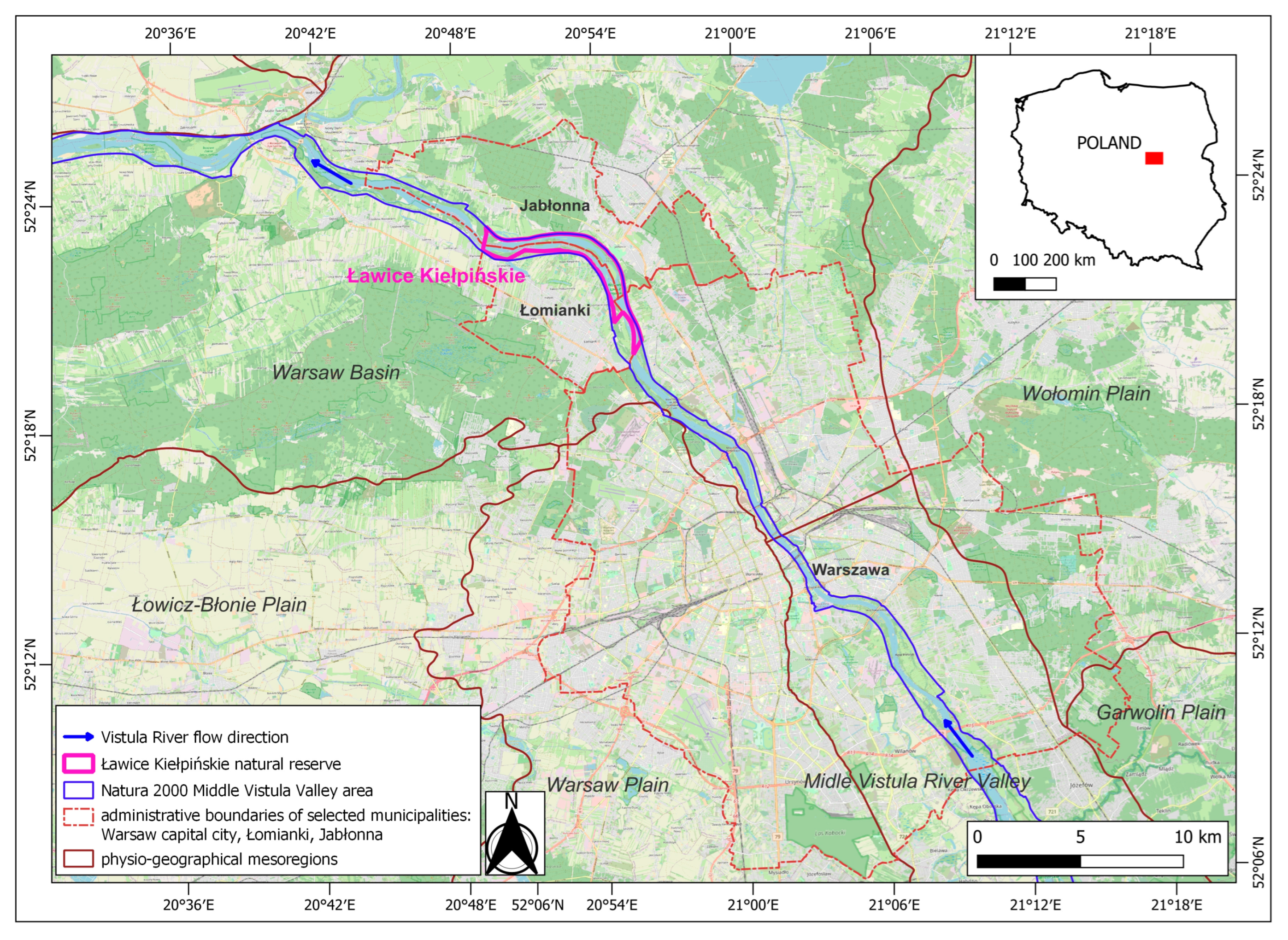
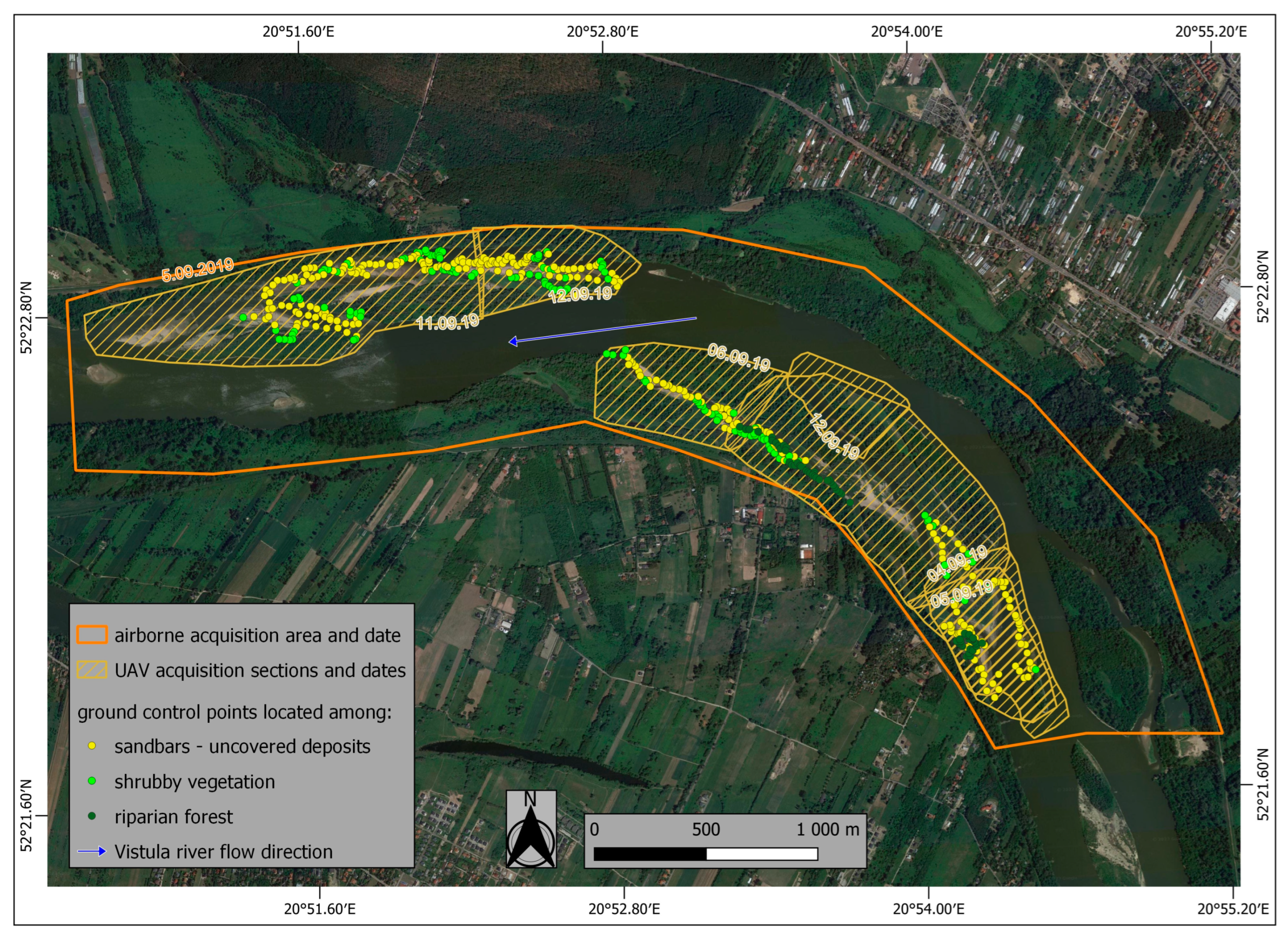
The main objective of this paper is to assess and compare the accuracy of state-of-the-art remote sensing (RS) technologies in generating DEMs at centimetre precision for fluvial landscape characterization and monitoring at a large scale. An airborne ALS campaign was flown to cover an area of about 3.0 square kilometres (km2). In the same period, an extensive multi-mission UAV campaign was performed over the same area, with UAV-LiDAR and RGB sensors, and an acquisition with Pléiades-1 in stereo mode was tasked. The field campaign was completed by a ground control points measurement campaign with the GNSS RTK system (GPS + GLONASS measurements), resulting in 516 points to be used for error assessment and comparison. These points were collected on the three main land-cover classes that shape the riparian corridor and that are of particular importance for river landscape monitoring: forest, shrubs, and sediment bars. The large amount of data collected allowed for an exhaustive comparison of LiDAR technology against DAP techniques acquired from either UAV or satellite (Pléiades in this case). Besides, UAV-LiDAR was assessed against airborne LiDAR. The findings of this assessment are extensively presented and discussed in the next sections of the presented paper.

2. Materials and Methods

2.1. Study Area

The study area is a lowland valley of a braided river (the Vistula River), located in the vicinity of a large urban agglomeration (the City of Warsaw, Poland), however, the selected river section is characterized by a natural riverscape shaped by almost freely acting processes of fluvial erosion and deposition. It is located a few kilometres north of Warsaw, i.e., downstream from the city, where the Vistula valley widens at the exit of the so-called Warsaw corset—a narrow reach similar to a gorge [33] (Figure 1). The widening of the valley floor is filled with the river terraces deposited during the last glaciation of the Pleistocene (Vistulian or Weichselian glaciation) and deposited relatively close (70 km) to the LGM (Last Glacial Maximum), but beyond its extent [34,35]. However, huge amounts of sand originating from the fluvioglacial environment of the LGM were transported just 10 km northerly from the study area through the LGM ice-marginal valley [35,36] and formed the body of the terraces together with fluvial sand coming from sections of the Vistula catchment in a periglacial environment. The dunes developed on these terraces in older and younger dryas (at the end of the Pleistocene), and afterward the Holocene floods eroded many traces, which are still visible on their surfaces, as in the case of the Vistula River with adjacent sections located upstream [33] and 50 km downstream [37].
The study area is part of a nature reserve called “Ławice Kiełpińskie” (“ławice” means shoals in Polish) (Figure 1). The reserve encompasses a set of riverine islands, sandbars, and broad channel bottoms covered by flowing waters, with a total area of 8.04 km2. The islands undergo strong natural erosion, and are undercut, especially in the vicinity of the main current of the river. The channel banks are also undercut by erosion, but with a somewhat lower intensity. Sandbars are transforming slowly into new islands, as a result of the accumulation of fluvial deposits, particularly fine sand.
Our study focuses on two islands located in the northern part of the reserve, in the municipality of Jabłonna, and two southern islands, located in the municipality of Łomianki. For the sake of simplicity, the two northern islands, which become connected at very low water levels, will henceforth be referred to as the “Northern Island”, and similarly, the two southern islands will be referred to as the “Southern Island” (Figure 2). The northern island has an area of approximately 0.5 km2 while the southern has an area of about 0.9 km2. The average elevation of the islands is 75 m above sea level, and while we were analysing the elevation of the terrain in geodetic heights (relative to the WGS 84 ellipsoid), the measured elevations of the islands are approx. 102–112 m, while the tree crowns on elevated parts of the islands reach geodetic heights of almost 150 m.
The dominating type of vegetation on the islands is typical of riparian plant communities. The edges of the islands and the depressions within the islands are covered by low vegetation (grasses, sedges) and young willow bushes (several years old). In some places, the vegetation develops in closed depressions (mudflats—slack-water deposits). Some of the shrubs on the islands, including in the higher parts, consist of dense and intensively developing goldenrod. In the oldest and most elevated parts of the islands, which have not been flooded for many years, there are riparian stands composed mainly of willows (including trees several decades old), in addition, with the participation of black and white poplar, and ash-leaf maple (considered as an invasive species). Recently, Da Silva et al. [39] explored the islands, identifying the major succession processes of plant communities occurring in sandy habitats and in wetter parts of the islands characterized by a dynamic balance of habitats.

2.2. Multi-Source Data Acquisition Campaign

The study described in this article focuses on assessing the accuracy of DTM/DSM models obtained from different sensors, mounted upon various flying platforms, hence having different technical parameters and different processing techniques. The main sensors and data collected in this study are:
  • Airborne LiDAR sensor and point cloud derived from laser scanning: herein referred to as ALS;
  • UAV LIDAR sensor and point cloud derived from laser scanning: herein referred to as UAV-LS or ULS;
  • RGB images taken from the UAV platform: herein referred to as UAV-DAP;
  • High-resolution satellite images acquired by Pléiades-1 satellite: herein referred to as PLEIADES.
Measurements taken from the UAV were supplemented by ground-based GNSS receiver measurements with an RTK station, for proper geo-referencing at centimetre accuracy.

2.2.1. UAV Flights

The main challenge of the envisaged acquisition campaign, consisted in covering the entire area of 3.0 km2 at the centimetre resolution with a UAV, in a relatively limited timeframe, i.e., during low water levels’ summer months, so as to ensure minimal changes in the fluvial sediments deposited on sandbars and islands.
The UAV data acquisition campaign for the computation of DEMs took place in September 2019. It was preceded by the two days of UAV flights in the middle of July and three days at the end of July and the beginning of August. Those first acquisitions were not covering the entire islands and they were done to test the instrument response and our mapping capability. The flights were repeated in September to cover the entire islands and to ensure simultaneity with the airborne acquisition (see Section 2.2.2). The data was collected during two days of field operations on the Northern Island (11–12 September) and during four days of fieldwork on the Southern Island (4–6 and 13 September) (Figure 3).
The characteristics of the flight carried out with the UAV (model DJI M600) were as follows: flight height up to 75 m above ground level, flight speed 5.5 m/s, distance between paths 45 m, flight time up to 17 min, and 2-4 flights per day.
The data acquired were:
  • Visible (RGB) images from a digital camera (APS-C) model Sony ILCE-6000, with 6000 × 4000 pixels (manufacturer: Sony, Tokyo, Japan)
  • LiDAR (laser detection and ranging) data from the laser sensor Velodyne VLP-16, −15° to +15° vertical FOV, 360° horizontal FOV, with a density of ∼50 points m−2 (manufacturer: Velodyne Lidar, San Jose, CA, USA).
Overall, an area of about 300 ha was covered with LIDAR point clouds with an accuracy of >100 pts/m, as well as with RGB images at 5 cm resolution. These images were used in the post-processing stage to colour the point clouds and also to compose an orthophotomap and a digital elevation model, based on the digital photogrammetric technique (as described in Section 2.3).

2.2.2. Airborne Flights

Airborne flight with ALS and RGB + CIR camera imaging was carried out by the company OPEGIEKA Ltd (Figure 3). The flight was carried out on 5 September 2019 after good weather conditions were confirmed. In the case of LiDAR measurements, data were acquired using a RIEGL VQ-1560i-DW laser scanner (manufacturer: RIEGL, Horn, Austria) operating at an infrared wavelength of 1.064 nm, and at a green wavelength of 532 nm, integrated with RGB and colour infrared (CIR) aerial imagery, hence both point clouds were made available for this study. On board the twin-engine Vulcanair P68 SP-OPG aircraft, all sensors including the GNSS/IMU positioning system were mounted on the same stabilised bed. The subsequent data georeferencing process included the alignment of image series with Riegl software (RiPROCESS, RiWORLD) for both images and LiDAR point clouds.

2.2.3. Satellite Data

Satellite data used in this study to create digital elevation models in stereo mode were acquired from Pléiades satellites operated by the French Space Agency (CNES) and Airbus Defence and Space Intelligence. Pléiades 1A and Pléiades 1B images are acquired in panchromatic (0.47–0.83 µm), blue (0.43–0.55 µm), green (0.50–0.62 µm), red (0.59–0.71 µm), and near-infrared (NIR) (0.74–0.94 µm) spectral bands.
The resolution of final products (primary, projected, and orthophoto) is 0.5 m for the panchromatic images and 2 m for multispectral images. The Pléiades system offers high-resolution stereoscopic coverage capability, which allows for DEM extraction and DSM to DTM conversion. Therefore, for the purpose of this paper, a digital surface model (DSM) was derived from high-resolution Pléiades 0.5 m panchromatic tri-stereo pairs of images.

2.2.4. Field GCPs for Comparative Assessment

A network of ground control points (GCPs) was collected in the field and used as ground truth reference to verify the heights of digital terrain models obtained from multiple data sources (UAV, ALS, and satellite data). A GNSS receiver with an RTK station (GPS + GLONASS measurements) was used, for which the assumed accuracy of the height measurement error is ±2–3 cm [40]. The alignment of a special marker on the GNSS pole was always verified to control and mitigate the problem of the sharp tip of the pole penetrating too much into the ground. Moreover, the pole was not placed in locations with terrain considered too soft for the measurement.
The collected ground control points (GCPs) represent different riverscape areas: (1) “sediment”: uncovered sandy deposits—sandbars from a geomorphological point of view, (2) “shrub”: low shrubby vegetation—a higher level of sandbars, which is transforming into riverine islands, and (3) “forest”: islands significantly elevated upon the water level in the channel with mature riparian forest on their surface. Of the 516 spatially distributed GCPs (Figure 3), 297 points were collected on “sediment” sandbars, while 153 were collected on “shrub” vegetation (up to about 1–1.5 m high) and finally 66 on “forest” areas. The GCPs were not collected on channel banks and islands’ banks (alluvial escarpments with quite steep slopes), and not measured at the bottom of the active river channel with flowing water or on the floodplain outside the reach of the islands.
The graph below (Figure 4) presents changes in the water level within the period of our data acquisitions at the Warsaw “Bulwary” water gauge (the closest automatic water gauge to our study area, located upstream of the river). The water gauge is located at 513.3 km of the Vistula River, with the water gauge ordinate set at 76.08 m above sea level. As can be seen, airborne and UAV acquisitions were made during similar very low water levels (42–52 cm above the “0” water level gauge). It should be noted that the lowest water level at the “Bulwary” water gauge associated with the hydrological drought was 26 cm (recorded in 2015 and then in August 2018), so during our measurements we were experiencing very similar conditions. Besides, the warning level at this water level gauge is shown at 600 cm and the alarm level at 650 cm. Thus, changes in water levels had a negligible effect on the geomorphology of the islands and sandbars during this short, 10-day period in September 2019. Besides, the fact of collecting GNSS-RTK measurements only on homogenous flat areas of at least 2 m × 2 m, situated away from the riverbed, ensured a negligible effect on our measurements, hence on the proposed DTM comparative assessment.

2.3. Data Processing

Dedicated software from GreenValley International was used to process the LiDAR data acquired from the UAV platform—LiAcquire for georeferencing the point cloud and pre-processing, and LiDAR 360 for data processing to obtain DTM/DSM products. AGISOFT Metashape software was instead used to produce orthophotos and DTMs/DSMs from the RGB camera images. The processing workflow is described step-by-step herein and illustrated in Figure 5. The use of LiAcquire allowed georeferencing of point clouds with base station coordinates. The original trajectories of the individual flights were used for geographic referencing using the base station log file and the measured GNSS position. Camera positions for the acquired RGB imagery were saved using LiAcquire. The results are precisely georeferenced point clouds.
Point cloud analysis was then carried out in LiDAR 360 (manufacturer: Green Valley International, Beijing, China). Strip alignment was performed for each flight, in order to correct for boresight error caused by the offset of the laser scanner and IMU coordinate system. The procedure of removing outliers from point clouds was also performed. The merging of the results of single flights into one file for each island was then carried out. The next step was ground point classification, i.e., deciding whether the obtained points bearing geographic coordinates represent laser reflectance values from exposed terrain, vegetation cover, or possibly anthropogenic objects. Air points classification was also performed, i.e., a procedure of removing air outliers, which can be caused, for example, by aerosol and suspended particles or objects flying in the air (e.g., birds). The pre-processing was completed by generating a point density analysis report.
Visualisation of the point clouds (obtained from the UAV-LiDAR data) by assigning a hypsometric colour scale to the elevation points of the land cover and displaying profile graphs for the selected cross-sections of the islands enabled a preliminary height analysis (Figure 6). Further processing of the point clouds was then performed to obtain DSMs, followed by extraction of DTMs.
RGB images from the camera mounted on the UAV were processed in AGISOFT Metashape to produce orthophotomaps. The images were oriented using the camera positions and based on the ground control points measured with GNSS-RTK. The bundle adjustment with a self-calibration process was performed using GCPs and the images’ position provided by drone navigation sensors. Merging data from several acquisitions (flights) was needed to compose the orthomosaics. Using photogrammetric methods, the orthophotomaps were processed into DSMs with selected resolutions.
For the airborne data, the pre-processing of the data to obtain both the georeferenced point cloud from the laser scanning and the photogrammetric products (used in the final step to colourise the point cloud with RGB attributes from digital photos) was performed by OPEGIEKA Ltd. The software used to classify the LiDAR point cloud was: TerraScan and TerraModeler (TerraSolid), RiHYDRO (Riegl). The classification process of the laser point cloud can be divided into 3 stages: automatic classification (using an appropriate sequence of filtering algorithms), manual classification (to control the effectiveness of the automatic classification and supplement it), and additionally classification of bathymetric data. Specifically, the automatic classification process included the classification of air points by removing outliers, and the classification of ground points, using the progressive TIN densification algorithm [41].
In the case of the Pléiades satellite imagery, standard photogrammetric techniques applied to several optical images were used to derive the DEMs. ERDAS Imagine Auto DTM software was used for this purpose. Image parallaxes between the conjugate points on the overlapping images of the remote sensing stereo datasets were measured to calculate the elevations of pixels. The image matching algorithms allowed to provision for initial parallax with high accuracy.
Interpolation techniques such as Kriging and TIN (triangulated irregular network) with variable parameters were tested and used to obtain an appropriate level of detail of all DEMs, given the available computing power. Kriging, under suitable assumptions of the prior covariances, gives the best linear unbiased prediction at unsampled locations. The main strengths of Kriging are in the statistical quality of its predictions (e.g., unbiasedness) and in the ability to predict the spatial distribution of uncertainty [42]. It provides particularly well-looking results with fairly evenly distributed measurement points. While it might be not optimal in terrain with significant differences in local variations (abrupt changes and break lines), this is not the case of our area. Therefore, Kriging interpolation was used in the end to generate the DSMs.
Using a larger number of points for interpolation results in a correspondingly higher resolution of the resulting DSM, as well as DTM derived from it., e.g., 5 cm, 10 cm, 25 cm, and 40 cm. After several tests, the accuracy of 10 cm was chosen for all products, as a good compromise between the spatial resolution of different data sources and processing time. Only for the Pléiades model, was this not possible due to the resolution of panchromatic images limited to 0.5 m. Figure 7 presents an excerpt from DMSs obtained from four different platforms/sensors All DSMs encompass land cover heights in the range of approx. 100 to 150 m (in WGS-84 geodetic heights). Well visible are the differences in the resolution of the models, where both LiDAR models (ULS and ALS) visually perform the best, compared to the photogrammetric models. In particular, the structure of vegetation on the island is very well visible on DSMs generated from LiDAR point clouds.

2.4. Data Comparison and Methodology for Interpretation of Results

The performed comparison of DEMs was developed along two main aspects: (1) different platforms flying at different altitudes (UAV, aircraft, satellite), and (2) different methods of remote data acquisition, namely, laser scanning and digital aerial photogrammetry (DAP) using RGB imagery. The errors in elevation on generated DEMs (error comparisons) refer to the values of the field GCPs (described in Section 2.2.4).
The problem of comparing multiple data sources having different spatial resolutions was mitigated by using a buffer and averaging the height values assigned to all pixels falling within the buffer. Absolute errors were computed using different buffer values. A circle with a radius of a given value (0.5 m, 1 m, or 1.5 m) was drawn around a field GCP and an average value was calculated from the pixels included in this buffer. Comparing the value from the GNSS (as a reference) with the resulting value gave the magnitude of the DEM’s error at the specific point. The most meaningful results were obtained with the buffer of 1 m, hence it was retained as the final buffer value to be presented in this paper.
Absolute error values have been presented on boxplots and scatterplots. The graphs were produced using ggplot2—an open-source data visualization package for the statistical programming language R. “Box and whiskers plots” were plotted using Tukey’s method [43]. Each boxplot compactly displays the distribution of a continuous variable. It visualises the following summary statistics: the median—represented by a line in the middle of each box, two hinges—representing two quartiles of the error values in total, and two whiskers—representing two standard deviations of the error values in each direction (assuming a normal distribution of the data), as well as all “outlying” points individually. The arithmetic mean value of the absolute error has also been explicitly shown on the boxplots, as the value next to the small red arrow on each graph.
Moreover, we made a comparison of profile graphs drawn from the DTMs derived from different data sources. The profile graphs cross both islands. We drew them following three rules: lines of cross-sections are perpendicular to the current in the river channel, the lines cross through some of the highest and the lowest parts of islands in order to present their morphology, and the lines avoid any gaps in the field coverage by the DEMs used in the study.

3. Results

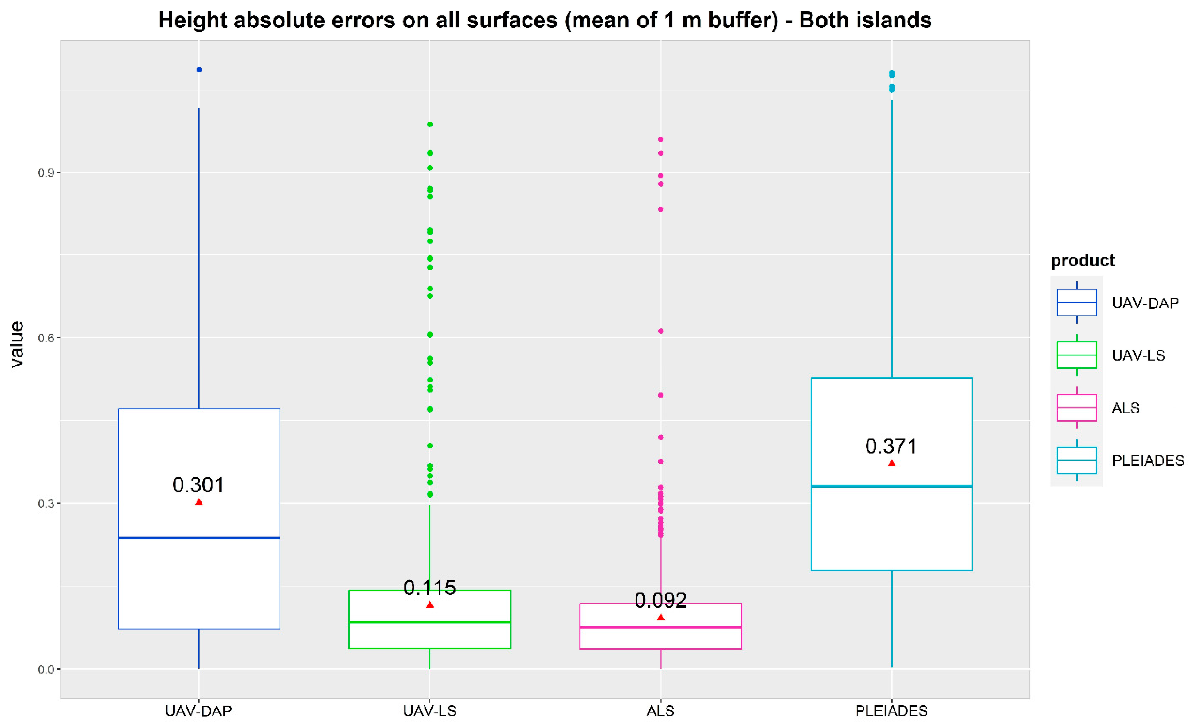
Figure 8 presents a first comparative assessment of mean height absolute errors of all DEMs made with the previously described platforms and sensors, namely: UAV-DAP, UAV-LS, ALS, and Pléiades. The lowest absolute errors were measured for airborne LiDAR data (ALS) with a mean error of 9.2 cm. Very similar accuracy was achieved by the UAV platform, where discrepancies from the field measurement average around 11.5 cm. The magnitudes of the standard deviation of the discrepancies are the smallest for DEMs generated from LiDAR data from both platforms, as compared to DAP techniques. In the case of the UAV-DAP photogrammetric model, the deviations are much larger. The second quartile of error values accommodates deviations in the order of 15 cm downwards relative to the median, while the third quartile of error values accommodates deviations of as much as 20 cm upwards relative to the median. The mean absolute error is 30 cm, however, the median error is a few centimetres less.
The photogrammetric model based on Pléiades imagery has the worst accuracy, carrying a mean absolute error of 37 cm and a median of around 33 cm, with the second quartile containing deviations of about 15 cm down from the median and the third quartile with deviations of more than 15 cm up from the median. On the other hand, the model extracted from the UAV-LS data relatively brings about the most outliers. They reach 80 cm or even more relative to the median. In second place in terms of the number of outliers is the ALS-derived DTM. In the latter case, however, the outliers are mostly clustered closer to the box and whiskers of the boxplot—predominantly with error values of around 30 cm (20 cm from the median), however in this case outliers that reach 80 cm can also be found.
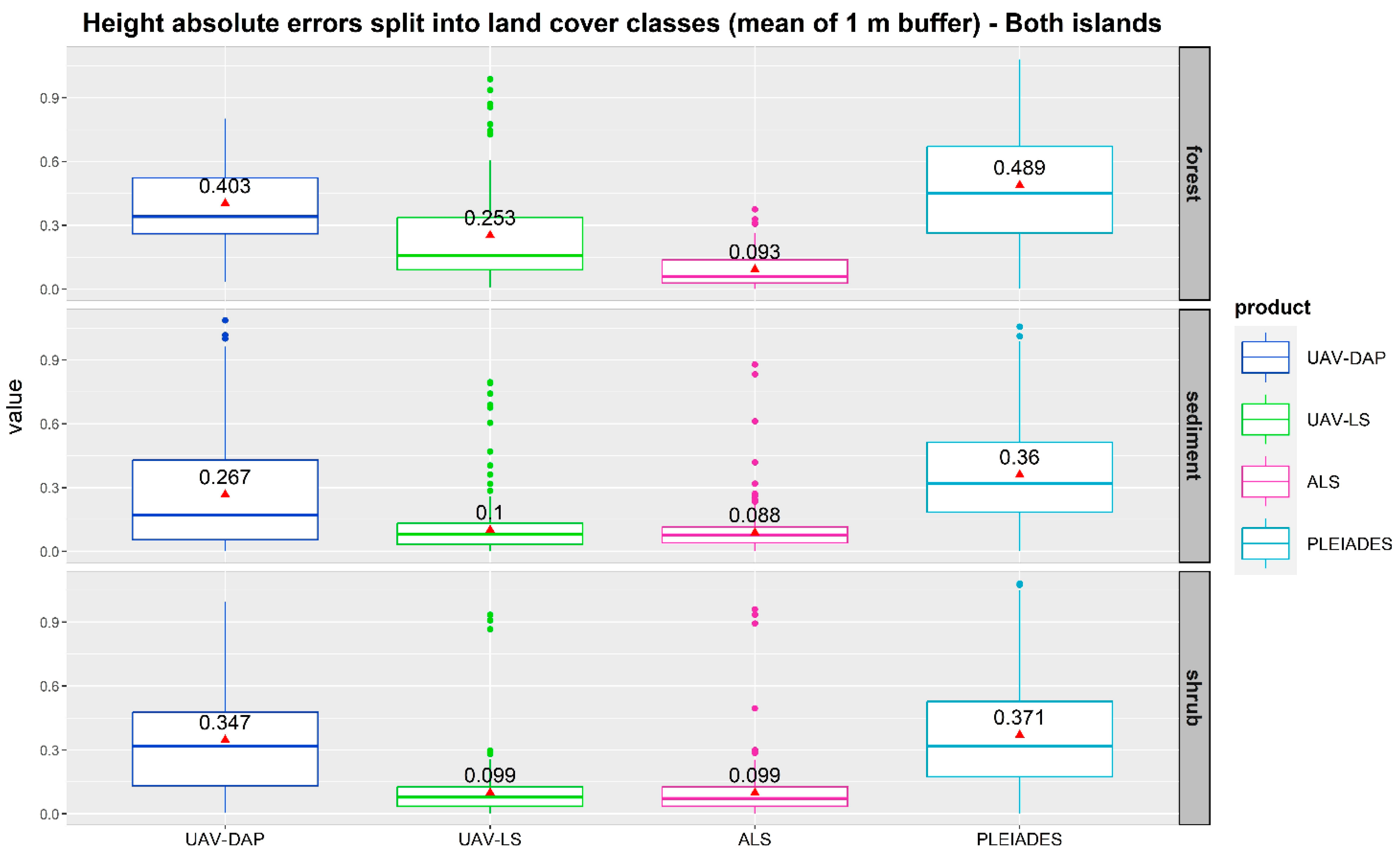
Figure 9 presents the results of the mean absolute error assessment, grouped by the different land cover classes that were sampled by the field GCPs. It confirms that the LiDAR-based DTMs are significantly more accurate when compared to DTMs obtained from DAP techniques, despite the platforms used and the land-cover types analysed. The UAV-LS or ALS-based DTMs perform way better than the UAV-DAP or Pléiades-based DTMs. Moreover, both LiDAR-based DTMs are very similar in terms of accuracy, underlying the similar precision of LiDAR sensors measurement.
The mean absolute error of the UAV-DAP model is 26.7 cm for the uncovered sandbars, 34.7 cm for shrub-covered areas, and 40.3 cm for the woods. In the meantime, the median error is only around 15 cm in sandy areas but reaching more than 30 cm in areas covered with shrubs or forest. This slight discrepancy between the mean and median indicates that for uncovered areas the errors are less numerous, but those that do occur, overestimate the measurement value more strongly (they are more deviate).
The mean absolute error of the UAV-LS model is 10 cm both for the uncovered sandbars and for the sites on islands with shrub cover, however, it exceeds 25 cm for the measurements in the woods. In the former case, there is almost no discrepancy between the mean and median errors, but in the latter, the median error is about 10 cm lower than the mean. Such a relationship indicates that DTMs derived from different input data and processing methods are characterised by a lower accuracy of ground terrain height measurements in places where the structure of the vegetation cover may interfere with ground imaging and height measurement.
On the other hand, the ALS DTM has an accuracy of 9.3 cm in the forest class, indicating the better capability of the ALS sensor to penetrate the vegetation canopy as compared to the UAV-LS sensor. This can be explained by the multi-reflectivity of ALS, which significantly increases the canopy penetration capacity compared to a single-beam scanner mounted instead on the UAV.
The LiDAR measurements generally bring a small standard deviation of error—DTM errors of a few centimetres are in the second and third quartiles (altogether making 50% of error values), only except for forest areas, where in the third quartile there are errors reaching about 15 cm above the median. The photogrammetric DTMs bring errors with larger standard deviations—in the third quartile there are errors reaching up to 30 cm from the median on uncovered sandbars and in the second quartile there are errors of around 20 cm below the median on shrubby areas. However, outliers of up to 1 meter (in the woods) or 80 cm (in the shrubs) relative to the median also occur for the UAV-LS model. This is due to the already-mentioned influence of vegetation cover.
The DTM obtained from ALS performs overall better than all the others, with an accuracy of around 9 cm for all validated land cover classes. In contrast, the DTM produced Pléiades imagery has a median error of as much as 36 cm for uncovered sandy sediments, 37 cm among the shrubs, and 49 cm among the woods. In all cases, the median error is almost the same as the mean (1–3 cm lower). The satellite model also yielded considerable standard deviations of error in the cases of all land cover classes (in the third quartile there are errors about 20 cm larger than the median, and in the second quartile there are errors about 15 cm smaller than the median).
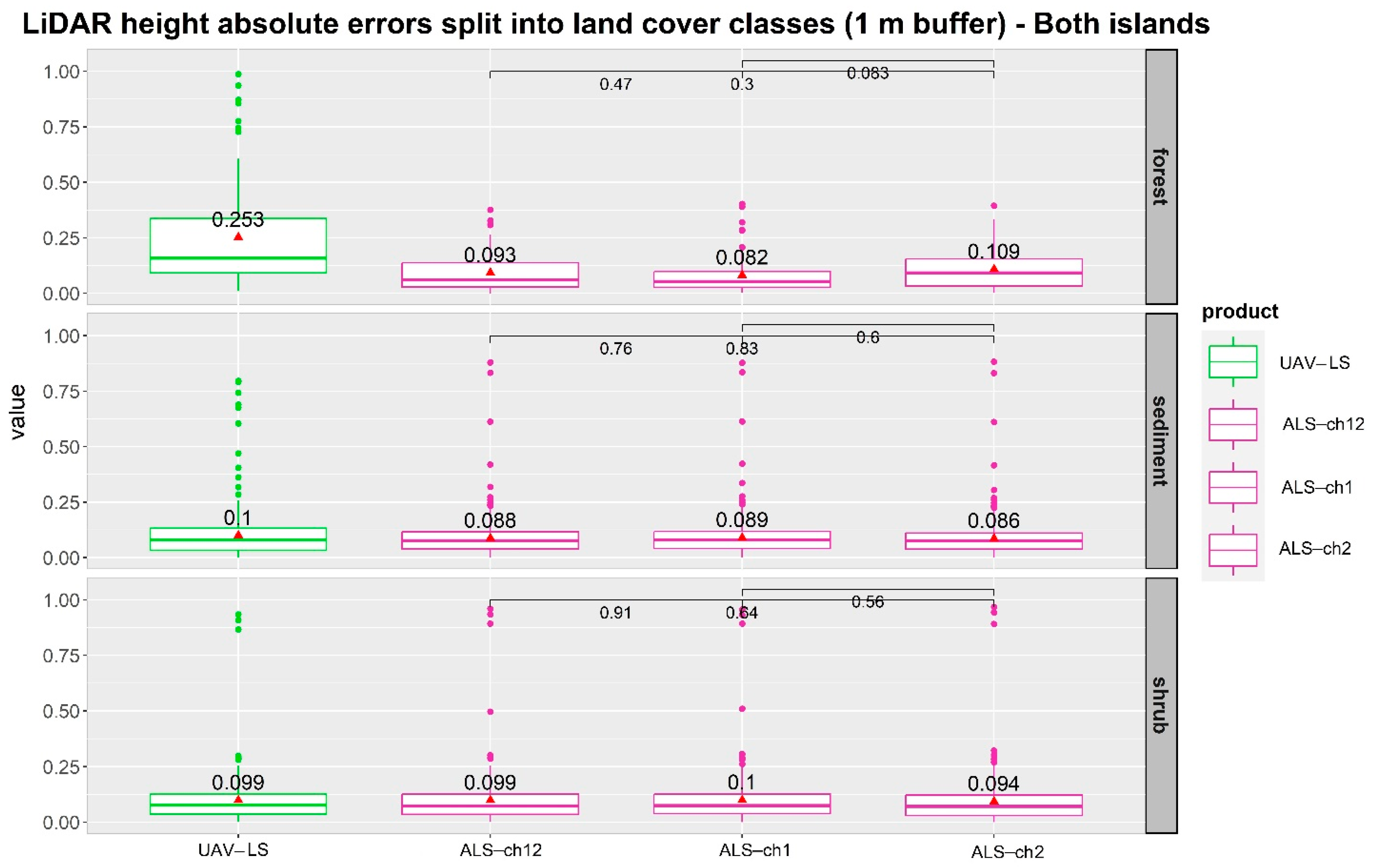
The last boxplot graph (Figure 10) compares the accuracy of DTMs obtained from the two LiDAR sensors, mounted on a UAV and an airplane, respectively. For the airborne-based LiDAR, the errors are presented for models obtained by using spectral channels 1 and 2, only channel 1, and only channel 2, respectively. This exercise aimed to check if the dual-channel LiDAR sensor might bring added value to the DTM computation, especially in penetrating the forest canopy.
The differences in the magnitude of the absolute error are small and very similar in most cases, ranging, for the ALS-based DTMs, between 8.2 and 10 cm for all land cover classes, despite the different spectral channel combinations used to obtain the models. The small error differences are confirmed by the statistical significance test (plotted in the graphs), which always give values above 0.05, hence demonstrating the non-statistical difference. The only significant difference occurs for the riparian forest areas, as previously reported in Figure 9, where the mean absolute error magnitude reaches 25 cm for the UAV-LS model, while for the ALS-derived models, it is within the limits of 8–11 cm.
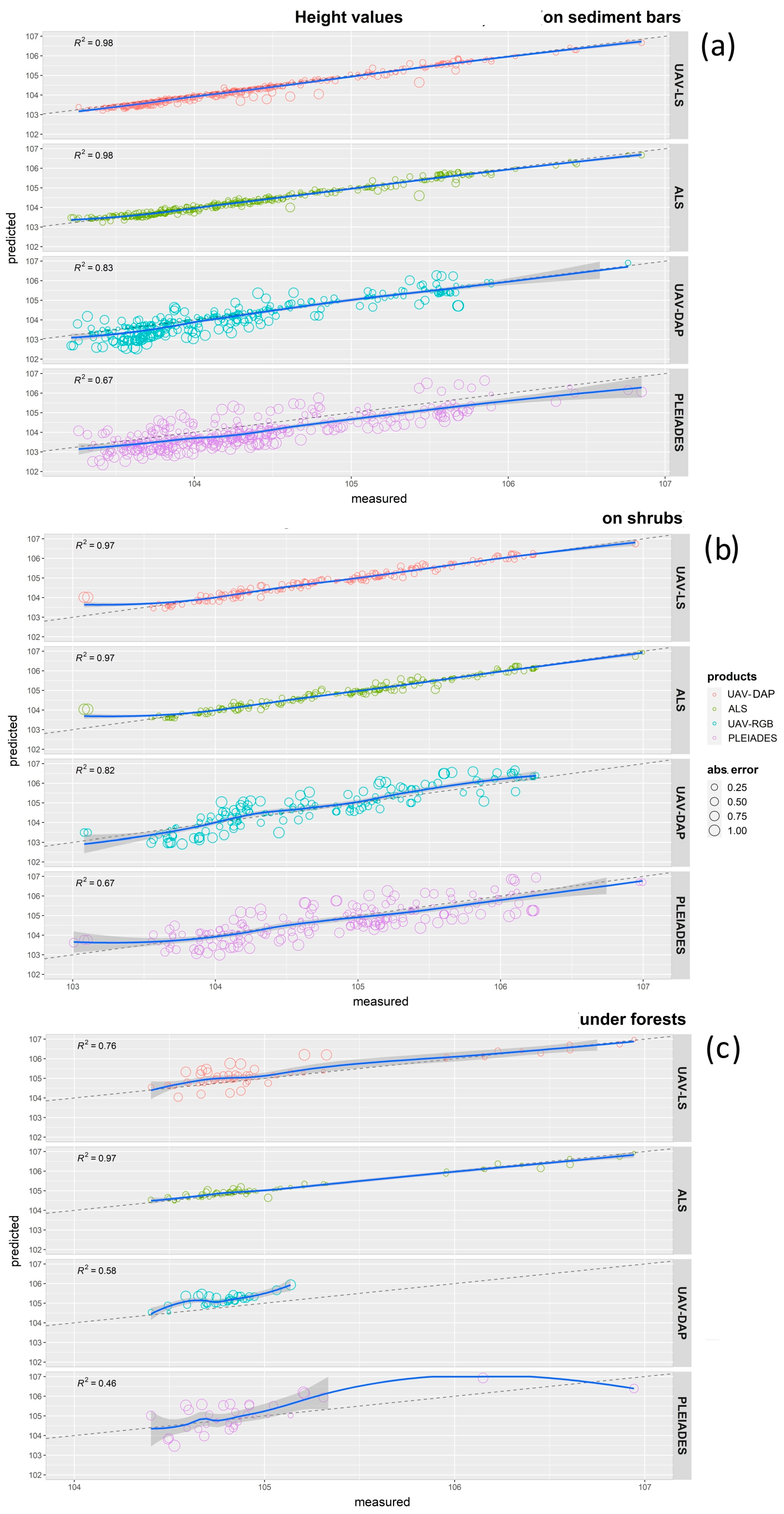
The scatterplots in Figure 11 show the distribution of predicted height values by different DTMs with respect to the distribution of heights, as measured in the field over the 516 GCPs. Results are plotted by the three different land cover classes.
For the sandbars (see Figure 11a), the curves have values with a very high fit to the linear function in the case of UAV-LiDAR and Airborne LiDAR, where in both cases R2 = 0.98, while the fit for the photogrammetric models is at a lower level: R2 = 0.83 for the UAV-DAP, and at only R 2 = 0.67 for the Pléiades. The highest frequency of high absolute error (0.5 m or more) is found for the Pléiades data, and secondly for the UAV-DAP data. It should also be noted that UAV-LS yielded a slightly higher number of such significant absolute errors than ALS.
Characteristics similar to the above are found in scatterplots for shrub-covered areas (Figure 11b), where the value of the fit of the regression curve to the linear function is: R2 = 0.97 both for ALS and UAV-LS, R2 = 0.83 for the UAV-DAP, and R2 = 0.67 for the satellite model. The only noticeable difference is that for the shrub class, individual observations bend the regression curves more for lower elevation values (for all models), although there are more measurements taken at lower elevations (exposed areas) on uncovered sandbars.
The forest patches (Figure 11c) yield quite different scatterplot characteristics. In this case, the ALS model has an almost perfect match with the ground measured values (R2 = 0.97), significantly ahead of the UAV-LS (R2 = 76), while significantly less accurate are the UAV-RGB (R2 = 0.58) and the Pleiades (R2 = 0.46), where we find numerous absolute error values deviating more than 50 cm or even more than 75 cm from the field GCPs.
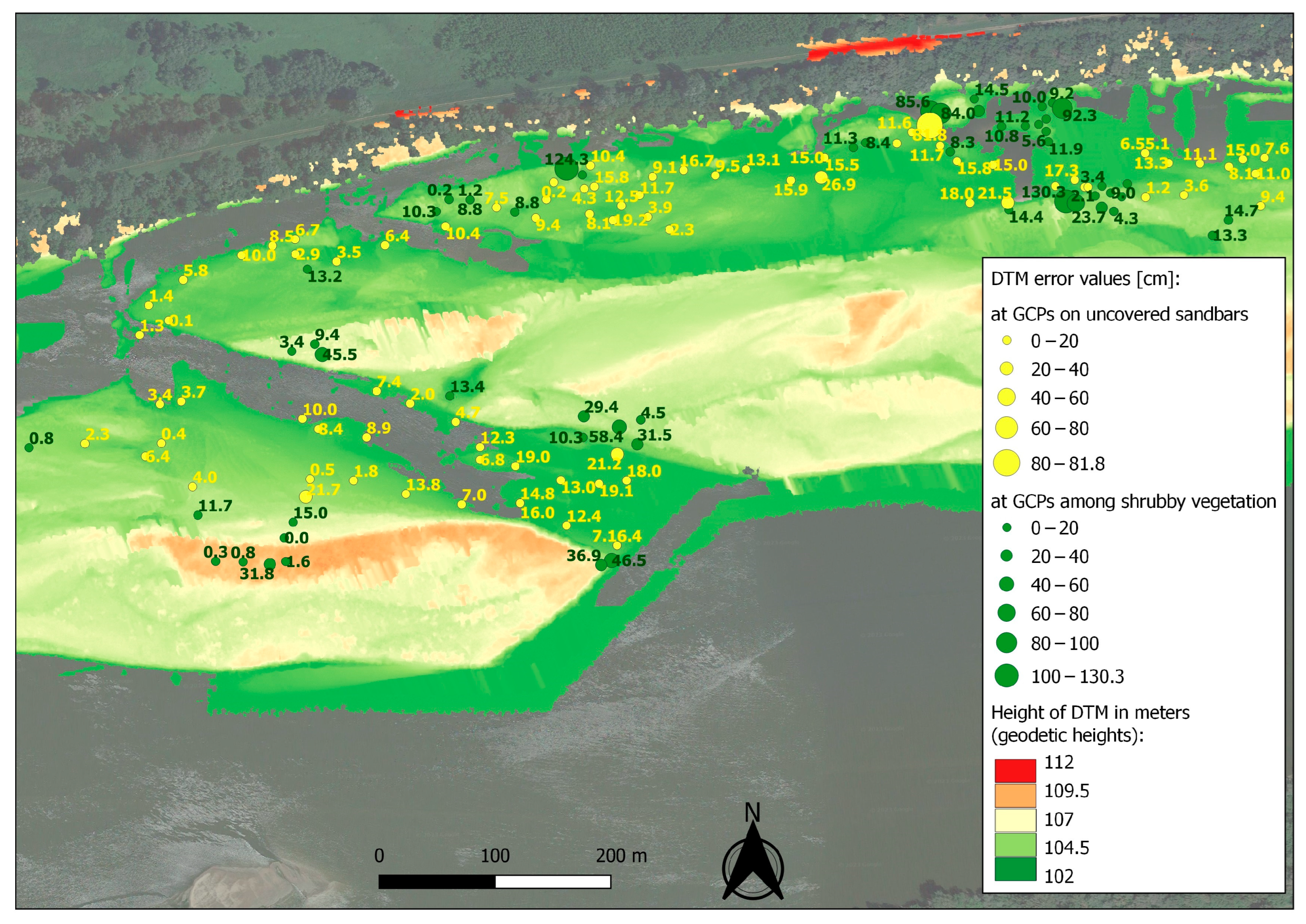
The spatial distribution of errors throughout the area is illustrated in Figure 12, for example, over the Northern Island (its central-western part) for the DTM derived from UAV-LiDAR data. There is a slight correlation visible between errors and locations—in terms of the height of terrain above the river water table, as well as vegetation cover or lack thereof. Namely, lower-lying sites on the exposed sandbars are characterised by small errors, for the vast majority of a few or a dozen centimetres, and in the island section presented here not reaching anywhere above 30 cm (except for one outlier). Meanwhile, among the GCPs distributed among the shrub vegetation on the islands, most errors are similarly low as for the uncovered sandbars, with a number of observations where the error magnitude approaches 0 cm, however, there are also a few outlier errors exceeding 80 cm or more.
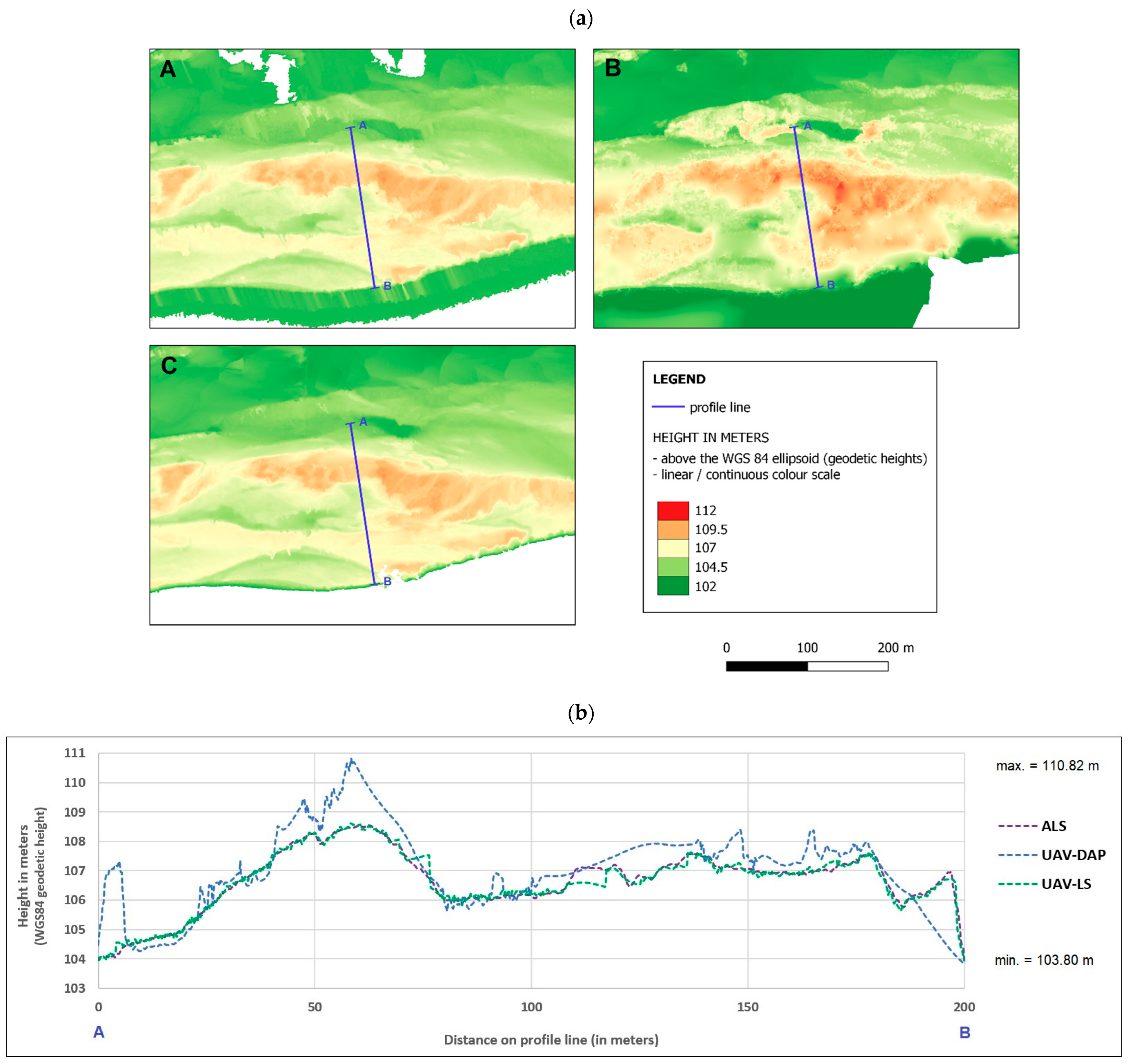
Finally, a profile graph comparison was made for the digital elevation models derived from different data sources in two selected and representative cross-sections of both islands. Figure 13a presents a cross-section for the Northern Island and Figure 13b shows the profile graph in this cross-section for both UAV-derived DTMs and the airborne DTM. 
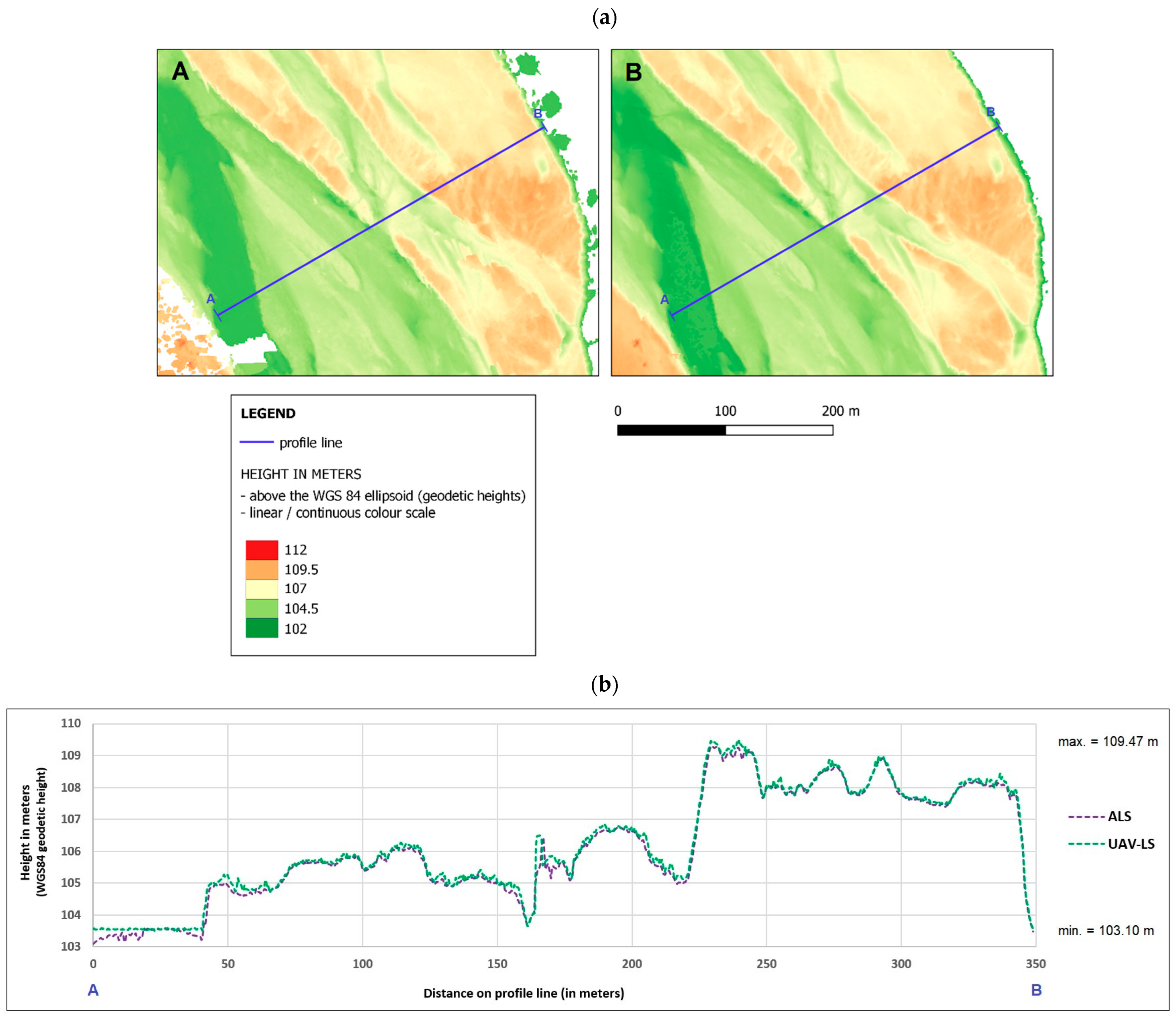
Figure 14a presents a cross-section for the Southern Island instead, and Figure 14b shows the profile graph in this cross-section only for the two LiDAR DTMs. Finally, 
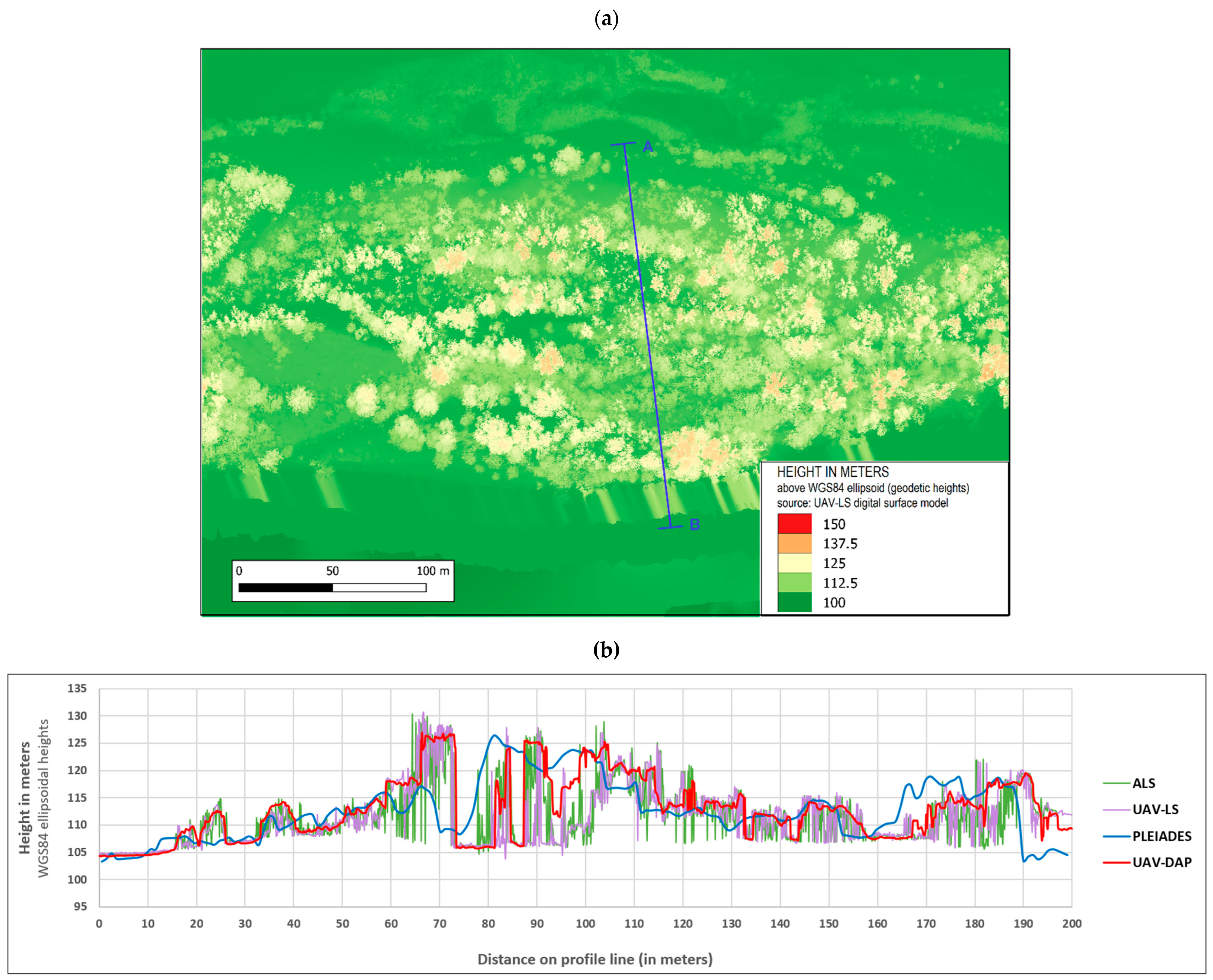
Figure 15a shows a cross-section of the Northern Island, for which a profile graph for four DSMs has been presented in Figure 15b.
The details of the profiles show that both LiDAR-derived DTMs (ALS and ULS) carry almost the same level of accuracy. While in Figure 13 they are compared with the UAV-DAP DTM, in Figure 14 only the terrain profiles from the laser scanning “point cloud” models are intentionally shown. Figure 13 reveals that the UAV-DAP model diverges much from the others, and usually overestimates, both in elevated places (island ridges)—on sediment bars with lots of shrubs and short vegetation—and in depressions, especially at the land-water boundary where elevation anomalies might occur as a result of the photogrammetric process.
Meanwhile, the comparison of the four DSMs presented in Figure 15 reveals similar problems on the water-land margin, especially for the Pléiades model. It can be seen that, on average, it exaggerates the height of the terrain (as shown earlier in Figure 8, Figure 9 and Figure 11) in the low-lying locations. On the other hand, the highest elevations on islands (their ridges) often have lower elevations on the satellite model than on the other DSMs. From the DSM-derived profile, a varied vertical structure of vegetation on the islands can also be seen. What is also particularly important and visible in Figure 15, as in Figure 14, is an almost perfect match between the ALS and UAV LiDAR measurements.

4. Discussion

When it comes to mapping the topography of the terrain, airborne laser scanning (ALS) currently still represents the “state-of-the-art” in terms of LiDAR sensor quality. However, in this paper we showed the potentialities of much cheaper UAV-based LiDAR sensors, being able to reach similar accuracies at a lower cost. Aircraft-based measurements and imaging may be considered more suited for regional scale surveys, while UAV is naturally better suited for local scale projects. The major advantage of UAVs is the flexibility of these platforms to acquire imagery data, especially for small to medium size areas (from less than 1 km2, up to 7 km2) [44]. When it comes to cost-effectiveness, UAVs might become competitive if they were operating at approximately 300 m above ground level, while at approximately 600 m altitude the piloted platforms lead to a lower cost of operation [45]. The problem is that the current aviation safety regulations often pose limitations to UAV operations. Although technological regulations in the field of UAVs increasingly improve the reliability of drones, there is still a human factor, i.e., mistakes caused by the operators, resulting in potential collisions with airplanes and man-made constructions. The appropriate adjustment of the law to the changing realities, including the elimination of unnecessary exclusions of areas from UAV operation is still a challenge.
The second aspect we considered was a comparison of measurements taken from the same flying platform but with different sensors: laser scanning and optical imaging in the RGB spectrum. According to the literature, LiDAR measurements have better accuracy than photogrammetry, especially in natural environments with dense vegetation, such as the forest ecosystems. UAV-DAP as a method for constructing of DTMs was evaluated by different authors as a less reliable technique compared to LiDAR, especially in the case of woodlands [17,26,27,29]. Our study confirms this, however to be specific—ULS performed worse than ALS due to the more limited capabilities of the scanner mounted upon the UAV in mapping dense, multi-level canopy.
In the case of low vegetation, we managed to reach twice the vertical accuracy criterion of the LiDAR digital terrain model assessed with RTK GPS and total station measurements as Stal et al. [46] reached with airborne laser scanning over meadows (20 cm). Salach et al. [28] indicate that DEM constructed based on UAV-DAP can be three times less accurate than a UAL-based DEM for an area with low vegetation. The difference obtained in our case study between LiDAR and photogrammetric method on sandy and low vegetation areas is in line with this value reported in [28]. In the case of grassland vegetation, UAV performs well as a data collecting platform (canopy height, biomass, and vegetation cover), however the “structure from motion” (SfM) approach to obtain an image-based point cloud is often used (matching pixels of overlapping images to reach the 3D structure of a concerned object) [47,48]. As Polat and Uysal [25] suggest, for relatively small study areas, UAV photogrammetry with SfM approach can even supply digital elevation models as accurate as airborne LiDAR. In their study, UAV-DAP DTM yielded the second most accurate result (RMSE) among the four ALS-based DTMs.
The whole area of the riverine islands is affected by dynamic geomorphological processes, such as bank erosion and overbank deposition, however, the deposition occurs there during floods only. Nevertheless, the collected height data came from a very short period of one summer season only, during very similar low water levels. For these reasons, we did not expect to see any significant impact of morphometric parameters (such as river slope, channel shape index, or exposition and angle of the slope forming the banks of the river channel and islands) on the distribution of errors.
It should also be highlighted that the higher accuracy of DTMs produced in our study from the LiDAR data is the result of using more points for interpolation compared to the photogrammetric elevation models. In other words, for digital elevation models with the same declared resolution, the point clouds from laser scanning are denser than the “image point clouds” that are an intermediate product in the photogrammetric process. To obtain higher density point clouds with photogrammetry, a much higher number of RGB images would be necessary, drastically increasing the number of flights required to cover such a large area, hence limiting de facto the realistic operability and usability of such technique for real large applications and operations, such as the one presented in this paper.
Simpson et al. [18] highlight the need for sufficiently dense distribution of ground control points for DTM extraction from ALS point clouds and their assessment in forest environments, especially in areas where undergrowth or ground cover vegetation is prevalent. For studies that require high DTM accuracy, it is recommended that extensive ground control points are used across a range of vegetation structures to assess the accuracy of DTMs, in order to account for biases caused by vegetation cover. Precautions for the greatest DTM errors should be taken in areas characterized by dense ground-cover vegetation since ground returns are most likely to be obscured here. These areas could easily be identified using even a simple canopy height model. Future studies should aim to quantify these DTM biases.
The authors of this paper find similar problem with UAV-LiDAR measurements in the dense forest canopy, namely, inability to collect reliable GNSS ground control points. The general observation is that only UAV-LiDAR and ALS-LiDAR are suitable for measuring the height of riparian vegetation, since with photogrammetry, using RGB images, only the tops of the trees can be seen. On the other hand, the vast majority of our field measurements (collecting ground control points) were taken among low vegetation and on surfaces of bare, newly deposited, so a full assessment of the quality of individual digital elevation models among the willow stands (the woods) on the islands is not possible.
The effective processing of the raw LiDAR data—data filtering, interpolation methodology, DEM resolution choice, LiDAR data reduction, and the subsequent generation of an efficient and high-quality DEM, remain a big challenge. One of the most critical and difficult steps is the classification of LiDAR points into ground and non-ground points [49]. However, the issues of selecting data processing procedures and algorithms to generate optimal DTMs—except for the basic choice of interpolation methods and model resolutions—were not analysed in detail in this article. This issue is a subject of other research and will also be of interest in future methodological studies planned by the authors.
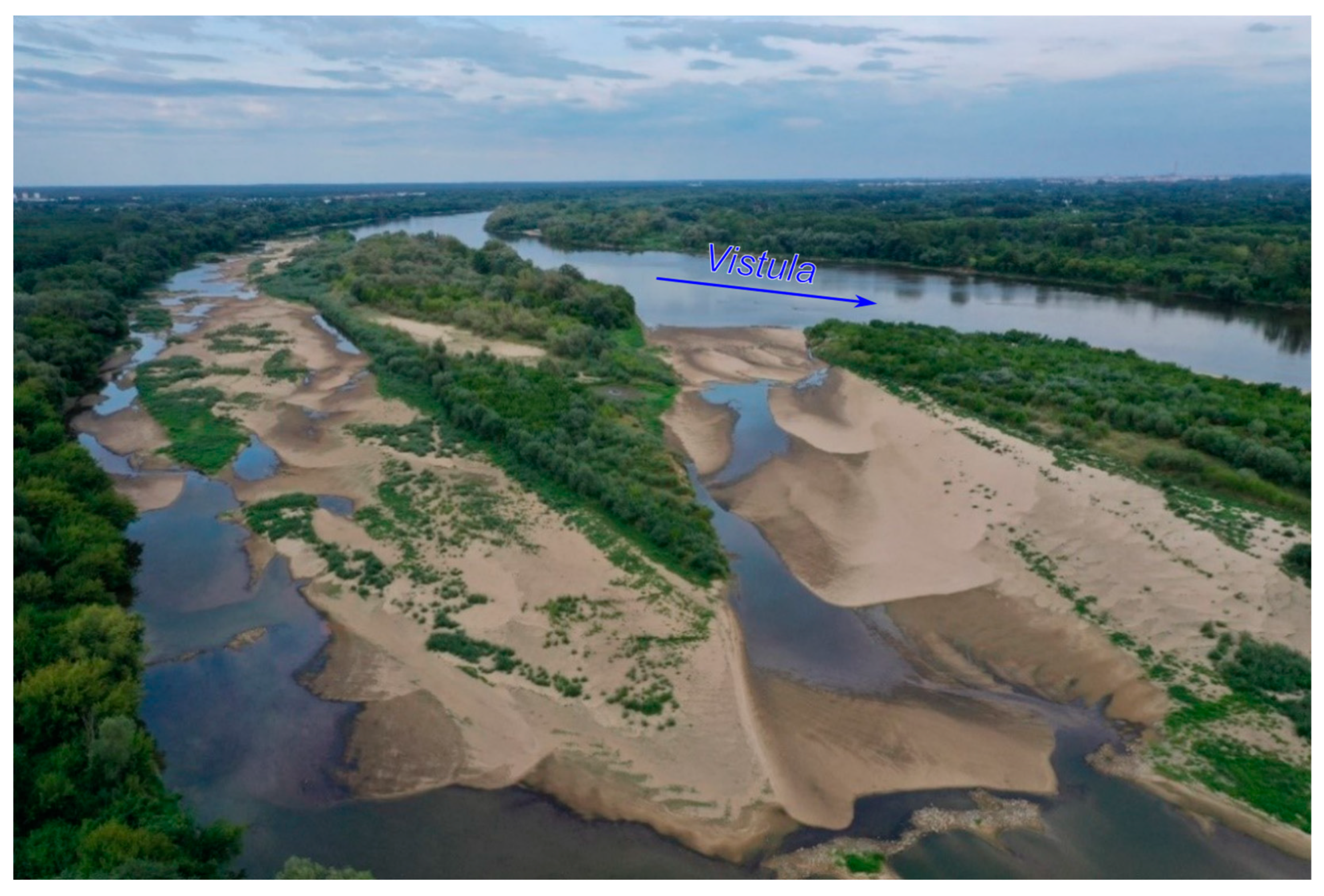
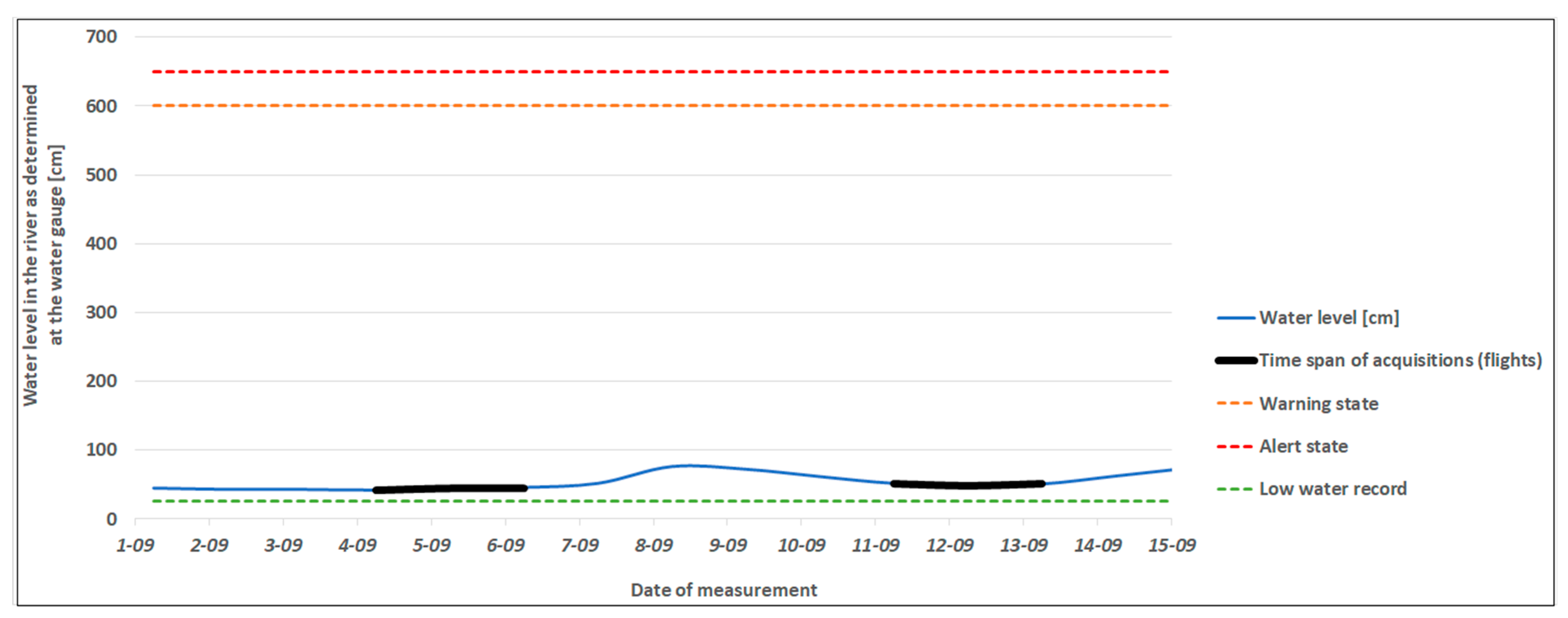
All the acquisitions of the data presented in this paper were performed during low water levels in the Vistula River. In such condition, four different geomorphological units can be distinguished as easily seen in the field: (1) floodplain above channel banks, (2) riverine islands, (3) sandbars, and (4) bottom of the active channel. From a geomorphological point of view, the most challenging goal is mapping the two lowest units, namely: (3) the sandbars and (4) the bottom of the active channel. Unfortunately, the active channel is completely covered by flowing water even at very low water stages. Sandbars (actually more elevated among those landforms) are exposed during low water stages, thus they can be surveyed by remote sensing. Repetitive measurement of sandbars enables determining the dynamics of these landforms and drawing further geomorphological implications, e.g., sediment budget calculation [50,51].
Geomorphological mapping of the channel heads in the headwater of the Vistula River in the Eastern Carpathians indicates that detailed morphometric analysis of small fluvial landforms is more accurate on the TLS (terrestrial laser scanning) DEM than ALS DEM [52]. In the case of our study area, it is a discussable opinion that TLS might be more suitable for mapping whole islands, however, small microforms, such as cut banks of the channel and especially cut banks of the islands, can indeed be better revealed with TLS scanning [53]. However, in an area the size of our case study we expect to obtain similar results with the use of ULS. It has been proved by Crespo-Peremarch et al. [29] that the ALS technique produces DEMs with an accuracy similar to those generated with TLS.
The origin of the studied islands is not related with floodplain excision, which forms a large and old island in an anabranching river [54], but rather with sandbar colonization by vegetation [55]. Assessment of different RS techniques for geomorphological purposes should therefore include an issue of projection of the vegetation on DEM [56]. According to the results of our study, in the case of geomorphological analysis of exposed sandbars, UAV–LiDAR seems to be the recommended option due to the dense point cloud it generates. Meanwhile, in order to show the structure of vegetation it is important to have good laser penetration and the possibility of multiple reflections, including the last one from the ground. The ability for canopy penetration of ALS seems to indicate it as the best technique in this respect.

5. Conclusions

The main conclusions are as follows. With the use of unmanned aerial vehicles (UAVs) we can obtain high quality measurements, however there are still several problems and limitations to overcome: (1) limited area coverage per single flight given the possible flight times, and the resulting labour intensity—resulting in a need to do many flights, as opposed to airborne missions which allow covering the same area in a much shorter time (e.g., 1 day of measurements vs. 1 week of measurements), (2) current national and international regulations for civil UAV operation, in particular, the allowed flight altitudes, (3) influence of the weather conditions on the measurement results and the need for their repetition—however this problem applies both to the drones and to the aircrafts, and (4) technical competitiveness of the sensors (laser scanners, cameras) mounted on airplanes and drones—although those fitted to UAVs are becoming increasingly better and almost comparable in quality to the sensors on aircrafts, at the same time bringing cost savings.
For the data analysed in this case study, i.e., a landscape dynamically shaped by fluvial processes, it shall be stated that digital elevation models based on laser scanning data (point clouds) give very good results, low absolute errors, and are more accurate than photogrammetric models. While the average absolute height error of the laser scanning DTMs oscillated around 8–11 cm for most surfaces (being higher only in forested areas), photogrammetric DTMs from UAV and satellite data gave errors averaging more than 30 cm. What is noticeable, airborne and UAV LiDAR measurements brought almost the perfect match. For the UAV-DAP model, the error was on average 25–40 cm and increased with the density and height of vegetation cover. The LiDAR measurements also brought a smaller standard deviation of errors compared to the photogrammetric DTMs. For example, for the ULS model, errors of a few centimetres accounted for 50% of error values for both uncovered sandbars and vegetated areas, while for the UAV-DAP model in the same 50% extent, there were errors deviating 20–30 cm from the median.
Despite the downsides of using UAV-LS for operational purposes described above, in this work it has been demonstrated that it is possible to generate DEMs over quite a large area of 3 km2, characterized by highly dynamic fluvial landscape, with a very high accuracy by using a much cheaper LiDAR instrument as compared to ALS. The generated DEMs over this area (especially large as for UAV mission) were assessed by a very solid validation campaign, consisting of more than 500 manually collected ground control points, resulting in an overall average error of only about 9 cm. Unfortunately, at the land-water margin, these results deteriorate, but not as drastically as for DEMs generated from RGB imagery, which was also expected due to the LiDAR limitations on water surfaces. At the same time, LiDAR-based models are also much better for penetrating tree-covered terrain, although in this study we only surveyed small forested areas, due to problems with accessibility and the loss of satellite signal under dense canopy cover.
To conclude, it can be expected that, given the high measurement reliability of this technology and the increasing operational capabilities of small civil UAVs and LiDAR sensors mounted upon them, this will potentially lead to their integration with other technologies to be deployed for operational monitoring of fluvial processes by river water authorities in charge of river geomorphological monitoring activities.

Author Contributions

Conceptualization, P.S. and L.D.; methodology, P.S. and L.D.; software, P.S., L.D. and J.C.; validation, P.S., L.D. and J.C.; formal analysis, P.S. and L.D.; investigation, P.S. and L.D.; resources, P.S., L.D., G.W. and J.C.; data curation, P.S. and L.D.; writing—original draft preparation, P.S.; writing—review and editing, L.D., G.W. and J.C.; visualization, P.S. and L.D.; supervision, J.C. and L.D.; project administration, L.D. and J.C.; funding acquisition, L.D. and J.C. All authors have read and agreed to the published version of the manuscript.

Funding

This work was supported by the National Science Centre, Poland (Narodowe Centrum Nauki), under the contract agreement UMO-2017/25/B/ST10/02967: Reach-scale hydromorphological characterization of European rivers using Hyperspectral and LiDAR data acquired from airborne and UAV platforms.

Data Availability Statement

The data collected and produced as part of this study are available in the authors’ resources. Pléiades satellite data are available from Airbus Intelligence upon specified request.

Acknowledgments

We would like to thank the following people: Maciej Góraj† and Piotr Babańczyk for their help in UAV data collection, Jacek Jóźwiak for technical support in data acquisition and processing, Kacper Pawłowski for the workflow presentation, Tomasz Lewicki for the delivery of hydrological data, Wojciech Ciężkowski for guidance concerning GIS and RS applications.

Conflicts of Interest

The authors declare no conflict of interest.

References

  1. Aggett, G.R.; Wilson, J.P. Creating and coupling a high-resolution DTM with a 1-D hydraulic model in a GIS for scenario-based assessment of avulsion hazard in a gravel-bed river. Geomorphology 2009, 113, 21–34. [Google Scholar] [CrossRef]
  2. Trevisani, S.; Cavalli, M.; Marchi, L. Surface texture analysis of a high-resolution DTM: Interpreting an alpine basin. Geomorphology 2012, 161–162, 26–39. [Google Scholar] [CrossRef]
  3. Bizzi, S.; Piégay, H.; Demarchi, L.; Van de Bund, W.; Weissteiner, C.J.; Gob, F. LiDAR-based fluvial remote sensing to assess 50–100-year human-driven channel changes at a regional level: The case of the Piedmont Region, Italy. Earth Surf. Process. Landf. 2019, 44, 471–489. [Google Scholar] [CrossRef]
  4. Li, Z.; Zhu, Q.; Gold, C. Digital Terrain Modeling: Principles and Methodology; CRC Press: Boca Raton, FL, USA, 2004. [Google Scholar] [CrossRef]
  5. Hirt, C. Digital Terrain Models. In Encyclopedia of Geodesy; Grafarend, E., Ed.; Springer: Cham, Switzerland, 2014. [Google Scholar]
  6. Maune, D.F.; Maitra, J.B.; McKay, E.J. Accuracy Standards & Guidelines. In Digital Elevation Model Technologies and Applications: The DEM Users Manual; Maune, D.F., Ed.; American Society for Photogrammetry and Remote Sensing: Bethesda, MD, USA, 2007; pp. 65–97. [Google Scholar]
  7. Sithole, G.; Vosselman, G. Experimental comparison of filter algorithms for bare-Earth extraction from airborne laser scanning point clouds. ISPRS J. Photogramm. Remote Sens. 2004, 59, 85–101. [Google Scholar] [CrossRef]
  8. Krauß, T.; Arefi, H.; Reinartz, P. Evaluation of selected methods for extracting digital terrain models from satellite born digital surface models in urban areas. In Proceedings of the SMPR2011, Tehran, Iran, 18–19 May 2011. [Google Scholar]
  9. Williams, R.D. DEMs of Difference. Geomorphol. Tech. 2012, 2, 1–17. Available online: https://www.researchgate.net/publication/310596075_DEMs_of_Difference (accessed on 29 March 2023).
  10. Panagiotakis, E.; Chrysoulakis, N.; Charalampopoulou, V.; Poursanidis, D. Validation of Pleiades tri-stereo DSM in urban areas. ISPRS Int. J. Geo-Inf. 2018, 7, 118. [Google Scholar] [CrossRef] [Green Version]
  11. Krauß, T. Preprocessing of satellite data for urban object extraction. In Proceedings of the International Archives of the Photogrammetry, Remote Sensing and Spatial Information Sciences—ISPRS Archives, Munich, Germany, 25–27 March 2015; Volume 40, pp. 115–120. [Google Scholar]
  12. Lefebvre, A.; Nabucet, J.; Corpetti, T.; Courty, N.; Hubert-Moy, L. Extraction of urban vegetation with Pléiades multiangular images. Remote Sens. Technol. Appl. Urban Environ. 2016, 10008. [Google Scholar] [CrossRef]
  13. Poli, D.; Caravaggi, I. 3D modeling of large urban areas with stereo VHR satellite imagery: Lessons learned. Nat. Hazards 2013, 68, 53–78. [Google Scholar] [CrossRef]
  14. Tsanis, I.K.; Seiradakis, K.D.; Daliakopoulos, I.N.; Grillakis, M.G.; Koutroulis, A.G. Assessment of Geoeye-1 stereo-pair-generated DEM in flood mapping of an ungauged basin. J. Hydroinform. 2014, 16, 1–18. [Google Scholar] [CrossRef]
  15. Bagnardi, M.; González, P.J.; Hooper, A. High-resolution digital elevation model from tri-stereo Pleiades-1 satellite imagery for lava flow volume estimates at Fogo Volcano. Geophys. Res. Lett. 2016, 43, 6267–6275. [Google Scholar] [CrossRef] [Green Version]
  16. Wang, R.; Zhang, S.; Pu, L.; Yang, J.; Yang, C.; Chen, J.; Guan, C.; Wang, Q.; Chen, D.; Fu, B.; et al. Gully erosion mapping and monitoring at multiple scales based on multi-source remote sensing data of the sancha river catchment, Northeast China. ISPRS Int. J. Geo-Inf. 2016, 5, 200. [Google Scholar] [CrossRef] [Green Version]
  17. Gil, A.L.; Núñez-Casillas, L.; Isenburg, M.; Benito, A.A.; Bello, J.J.R.; Arbelo, M. A comparison between LiDAR and photogrammetry digital terrain models in a forest area on Tenerife Island. Can. J. Remote Sens. 2013, 39, 396–409. [Google Scholar]
  18. Simpson, J.E.; Smith, T.E.L.; Wooster, M.J. Assessment of errors caused by forest vegetation structure in airborne LiDAR-derived DTMs. Remote Sens. 2017, 9, 1101. [Google Scholar] [CrossRef] [Green Version]
  19. Lind, L.; Hasselquist, E.M.; Laudon, H. Towards ecologically functional riparian zones: A meta-analysis to develop guidelines for protecting ecosystem functions and biodiversity in agricultural landscapes. J. Environ. Manag. 2019, 249, 109391. [Google Scholar] [CrossRef] [PubMed]
  20. Demarchi, L.; Bizzi, S.; Piégay, H. Regional hydromorphological characterization with continuous and automated remote sensing analysis based on VHR imagery and low-resolution LiDAR data. Earth Surf. Process. Landf. 2017, 42, 531–551. [Google Scholar] [CrossRef]
  21. Demarchi, L.; van de Bund, W.; Pistocchi, A. Object-based ensemble learning for Pan-European riverscape units mapping based on copernicus VHR and EU-DEM data fusion. Remote Sens. 2020, 12, 1222. [Google Scholar] [CrossRef] [Green Version]
  22. Gurnell, A.M.; Rinaldi, M.; Belletti, B.; Bizzi, S.; Blamauer, B.; Braca, G.; Buijse, A.D.; Bussettini, M.; Camenen, B.; Comiti, F.; et al. A multi-scale hierarchical framework for developing understanding of river behaviour to support river management. Aquat. Sci. 2016, 78, 1–16. [Google Scholar] [CrossRef] [Green Version]
  23. Carbonneau, P.E.; Piégay, H. Fluvial Remote Sensing for Science and Management; Willey-Blackwell: Hoboken, NJ, USA, 2012. [Google Scholar]
  24. Polat, N.; Uysal, M.; Toprak, A.S. An investigation of DEM generation process based on LiDAR data filtering, decimation, and interpolation methods for an urban area. Meas. J. Int. Meas. Confed. 2015, 75, 50–56. [Google Scholar] [CrossRef]
  25. Polat, N.; Uysal, M. An Experimental Analysis of Digital Elevation Models Generated with Lidar Data and UAV Photogrammetry. J. Indian Soc. Remote Sens. 2018, 46, 1135–1142. [Google Scholar] [CrossRef]
  26. Wallace, L.; Lucieer, A.; Malenovskỳ, Z.; Turner, D.; Vopěnka, P. Assessment of forest structure using two UAV techniques: A comparison of airborne laser scanning and structure from motion (SfM) point clouds. Forests 2016, 7, 62. [Google Scholar] [CrossRef] [Green Version]
  27. Goodbody, T.R.H.; Coops, N.C.; White, J.C. Digital Aerial Photogrammetry for Updating Area-Based Forest Inventories: A Review of Opportunities, Challenges, and Future Directions. Curr. For. Rep. 2019, 5, 55–75. [Google Scholar] [CrossRef] [Green Version]
  28. Salach, A.; Bakuła, K.; Pilarska, M.; Ostrowski, W.; Górski, K.; Kurczynski, Z. Accuracy assessment of point clouds from LiDAR and dense image matching acquired using the UAV platform for DTM creation. ISPRS Int. J. Geo-Inf. 2018, 7, 342. [Google Scholar] [CrossRef] [Green Version]
  29. Crespo-Peremarch, P.; Torralba, J.; Carbonell-Rivera, J.P.; Ruiz, L.A. Comparing the generation of DTM in a forest ecosystem using TLS, ALS and UAV-DAP, and different software tools. In Proceedings of the XXIV Congress of the International Society for Photogrammetry and Remote Sensing (ISPRS 2020), Online, 31 August–2 September 2020; Volume 43. [Google Scholar]
  30. Villanueva, J.R.E.; Martínez, L.I.; Montiel, J.I.P. DEM generation from fixed-wing UAV imaging and LiDAR-derived ground control points for flood estimations. Sensors 2019, 19, 3205. [Google Scholar] [CrossRef] [PubMed] [Green Version]
  31. Tamminga, A.; Hugenholtz, C.; Eaton, B.; Lapointe, M. Hyperspatial Remote Sensing of Channel Reach Morphology and Hydraulic Fish Habitat Using an Unmanned Aerial Vehicle (UAV): A First Assessment in the Context of River Research and Management. River Res. Appl. 2015, 31, 379–391. [Google Scholar] [CrossRef]
  32. Woodget, A.; Maddock, I.; Habit, E.; Visser, F. High Resolution Remote Sensing from a UAV for Quantifying Fluvial Topography. In Proceedings of the Ecohydrology/Hydroecology Meeting of the British Hydrological Society, Birmingham, UK, 17 April 2013. [Google Scholar]
  33. Wierzbicki, G.; Ostrowski, P.; Bartold, P.; Bujakowski, F.; Falkowski, T.; Osiński, P. Urban geomorphology of the Vistula River valley in Warsaw. J. Maps 2021, 17, 170–185. [Google Scholar] [CrossRef]
  34. Narloch, W.; Phillips, E.R.; Piotrowski, J.A.; Ćwiek, M. Patterns of deformation within a subglacial shear zone: Implications for palaeo-ice stream bed evolution. Sediment. Geol. 2020, 397, 105569. [Google Scholar] [CrossRef]
  35. Wierzbicki, G.; Grygoruk, M.; Grodzka-łukaszewska, M.; Bartold, P.; Okruszko, T. Mire development and disappearance due to river capture as hydrogeological and geomorphological consequences of LGM ice-marginal valley evolution at the Vistula-Neman watershed. Geosciences 2020, 10, 363. [Google Scholar] [CrossRef]
  36. Mojski, J.E. Przeglądowa Mapa Geomorfologiczna Polski 1:500,000; Arkusz Warszawa, IGiPZ PAN: Warszawa, Poland, 1980. [Google Scholar]
  37. Wierzbicki, G.; Ostrowski, P.; Falkowski, T. Applying floodplain geomorphology to flood management (The Lower Vistula River upstream from Plock, Poland). Open Geosci. 2020, 12, 1003–1016. [Google Scholar] [CrossRef]
  38. Solon, J.; Borzyszkowski, J.; Bidłasik, M.; Richling, A.; Badora, K.; Balon, J.; Brzezińska-Wójcik, T.; Chabudziński, Ł.; Dobrowolski, R.; Grzegorczyk, I.; et al. Physico-geographical mesoregions of Poland: Verification and adjustment of boundaries on the basis of contemporary spatial data. Geogr. Pol. 2018, 91, 143–170. [Google Scholar] [CrossRef]
  39. da Silva, A.R.; Demarchi, L.; Sikorska, D.; Sikorski, P.; Archiciński, P.; Jóźwiak, J.; Chormański, J. Multi-source remote sensing recognition of plant communities at the reach scale of the Vistula River, Poland. Ecol. Indic. 2022, 142, 109160. [Google Scholar] [CrossRef]
  40. Lovell, J.L.; Jupp, D.L.B.; Culvenor, D.S.; Coops, N.C. Using airborne and ground-based ranging lidar to measure canopy structure in Australian forests. Can. J. Remote Sens. 2003, 29, 607–622. [Google Scholar] [CrossRef]
  41. Axelsson, P. Processing of laser scanner data—Algorithms and applications. ISPRS J. Photogramm. Remote Sens. 1999, 54, 138–147. [Google Scholar] [CrossRef]
  42. Mitas, L.; Mitasova, H. Spatial Interpolation. In Geographical Information Systems: Principles, Techniques, Management and Applications; GeoInformation International: Cambridge, UK, 1999; Volume 1. [Google Scholar]
  43. Tukey, J.W. Box-and-Whisker Plots. In Exploratory Data Analysis; Addison-Wesley: Reading, MA, USA, 1977; pp. 39–43. [Google Scholar]
  44. Leitão, J.P.; Moy De Vitry, M.; Scheidegger, A.; Rieckermann, J. Assessing the quality of digital elevation models obtained from mini unmanned aerial vehicles for overland flow modelling in urban areas. Hydrol. Earth Syst. Sci. 2016, 20, 1637–1653. [Google Scholar] [CrossRef] [Green Version]
  45. Jeunnette, M.N.; Hart, D.P. Remote sensing for developing world agriculture: Opportunities and areas for technical development. In Proceedings of the Remote Sensing for Agriculture, Ecosystems, and Hydrology XVIII, Edinburgh, Scotland, 26–28 September 2016; Volume 9998. [Google Scholar]
  46. Stal, C.; Nuttens, T.; Bourgeois, J.; Carlier, L.; De Maeyer, P.; De Wulf, A. Accuracy Assessment of a Lidar Digital Terrain Model by using RTK GPS and Total Station. EARSeL eProc. 2010, 10, 1–8. [Google Scholar]
  47. Zhang, H.; Sun, Y.; Chang, L.; Qin, Y.; Chen, J.; Qin, Y.; Du, J.; Yi, S.; Wang, Y. Estimation of grassland canopy height and aboveground biomass at the quadrat scale using unmanned aerial vehicle. Remote Sens. 2018, 10, 851. [Google Scholar] [CrossRef] [Green Version]
  48. Théau, J.; Lauzier-Hudon, É.; Aubé, L.; Devillers, N. Estimation of forage biomass and vegetation cover in grasslands using UAV imagery. PLoS ONE 2021, 16, e0245784. [Google Scholar] [CrossRef]
  49. Liu, X.; Zhang, Z.; Peterson, J.; Chandra, S. LiDAR-derived high quality ground control information and DEM for image orthorectification. Geoinformatica 2007, 11, 37–53. [Google Scholar] [CrossRef] [Green Version]
  50. Heritage, G.; Entwistle, N. Drone based quantification of channel response to an extreme flood for a piedmont stream. Remote Sens. 2019, 11, 2031. [Google Scholar] [CrossRef] [Green Version]
  51. Leonard, C.; Legleiter, C.; Overstreet, B. Effects of lateral confinement in natural and leveed reaches of a gravel-bed river: Snake River, Wyoming, USA. Earth Surf. Process. Landf. 2017, 42, 2119–2138. [Google Scholar] [CrossRef]
  52. Płaczkowska, E.; Cebulski, J.; Bryndza, M.; Mostowik, K.; Murawska, M.; Rzonca, B.; Siwek, J. Morphometric analysis of the channel heads based on different LiDAR resolutions. Geomorphology 2021, 375, 107546. [Google Scholar] [CrossRef]
  53. Kaczmarek, H.; Tyszkowski, S.; Bartczak, A.; Kramkowski, M.; Wasak, K. The role of freeze-thaw action in dam reservoir cliff degradation assessed by terrestrial laser scanning: A case study of Jeziorsko Reservoir (central Poland). Sci. Total Environ. 2019, 690, 1140–1150. [Google Scholar] [CrossRef] [PubMed]
  54. Leli, I.T.; Stevaux, J.C.; Assine, M.L. Origin, evolution, and sedimentary records of islands in large anabranching tropical rivers: The case of the Upper Paraná River, Brazil. Geomorphology 2020, 358, 107118. [Google Scholar] [CrossRef]
  55. Gurnell, A.M.; Bertoldi, W.; Francis, R.A.; Gurnell, J.; Mardhiah, U. Understanding processes of island development on an island braided river over timescales from days to decades. Earth Surf. Process. Landf. 2019, 44, 624–640. [Google Scholar] [CrossRef] [Green Version]
  56. Rusnák, M.; Goga, T.; Michaleje, L.; Šulc Michalková, M.; Máčka, Z.; Bertalan, L.; Kidová, A. Remote Sensing of Riparian Ecosystems. Remote Sens. 2022, 14, 2645. [Google Scholar] [CrossRef]
Figure 1. Location of the “Ławice Kiełpińskie” natural reserve in the context of Warsaw urban agglomeration. Background map: OpenStreetMap. Data sources: EEA/GDOŚ, GUGiK, Solon et al., 2018 [38], own elaboration.
Remotesensing 15 01949 g001
Figure 2. Study area within the “Ławice Kiełpińskie” reserve. Oblique photo taken from a UAV in July 2019 showing a panoramic view upstream, towards Warsaw: northern part located in the Jabłonna commune. Exposed sandbars and islands with varying levels of vegetation can be seen.
Remotesensing 15 01949 g002
Figure 3. Study area. Islands within the “Ławice Kiełpińskie” (“Kielpinskie Shoals”) natural reserve. Overlayed are acquisition sections of the airborne and UAV missions, and the distribution of ground control points from GNSS-RTK measurements. Background orthophotomap: Google Satellite.
Remotesensing 15 01949 g003
Figure 4. Changes in the water level at the Warsaw “Bulwary” water gauge within the period of UAV and airborne data acquisitions. Hydrological data provided by the Institute of Meteorology and Water Management (IMGW), courtesy of T. Lewicki.
Remotesensing 15 01949 g004
Figure 5. Flowchart of data processing as regards data obtained from the UAV platform—laser scanning point cloud processing and photogrammetric procedures, used to generate DEMs.
Remotesensing 15 01949 g005
Figure 6. Example of the UAV-LiDAR point cloud for the Southern Island, representing the heterogenous landscape characterized by different land covers of the studied islands. Visualization made in LiDAR 360 viewer.
Remotesensing 15 01949 g006
Figure 7. Digital surface models’ (DSMs) coverage and heights comparison (A = UAV-LS, B = UAV-DAP, C = ALS, D = PLEIADES) on the example of Northern Island of the “Kiełpińskie Shoals”. Resolution of the models is always 10 cm, except for the Pléiades model (50 cm).
Remotesensing 15 01949 g007
Figure 8. Accuracy of DTMs generated from data from different platforms and sensors: unmanned aerial vehicle (UAV-LiDAR and UAV-DAP), aircraft (ALS), and Pléiades satellite (DAP–RGB images).
Remotesensing 15 01949 g008
Figure 9. Accuracy of DTMs generated from data from different platforms and sensors, grouped by different land cover classes: unmanned aerial vehicle (LiDAR and DAP techniques), aircraft (ALS–LiDAR), and Pléiades satellite (DAP–RGB images).
Remotesensing 15 01949 g009
Figure 10. Accuracy of DTMs generated from LiDAR data obtained from UAV platform and from the aircraft (ALS) in two spectral channels separately and combined. The comparison is grouped by the different land cover classes analysed.
Remotesensing 15 01949 g010
Figure 11. Scatterplots of height values generated on DTM according to different data sources (from top: UAV-LiDAR, ALS—airborne LiDAR, UAV—RGB photogrammetry, satellite images from Pléiades), and according to land cover classes ((a)—uncovered sandbars, (b)—shrub vegetation, (c)—riparian forest). The measurement values are in meters, WGS84 ellipsoidal (geodetic) heights.
Remotesensing 15 01949 g011
Figure 12. DTM visualization of the Northern Island (central-western section) with height error values at the GCP locations. Digital elevation model based on laser scanning from UAV (ULS). GCPs shown correspond to two vegetation and geomorphological classes: (1) shrub vegetation on the riverine islands and transforming higher level of sandbars, (2) uncovered sandy deposits on sandbars. Background orthophotomap: Google Satellite (with partial transparency).
Remotesensing 15 01949 g012
Figure 13. (a) Northern Island cross-section used to make the profile graph, image A—ALS, image B—UAV-DAP, image C—UAV-LS (ULS), (b) Northern Island—profile lines comparing three digital terrain models (DTMs). The measurement values are in metres, WGS84 ellipsoidal (geodetic heights).
Remotesensing 15 01949 g013
Figure 14. (a) Southern Island cross-section used to make the profile graph, image A—ALS, image B—UAV-LS, (b) Southern Island—profile lines comparing two LIDAR-based digital terrain models (DTMs). The measurement values are in metres, WGS84 ellipsoidal (geodetic heights).
Remotesensing 15 01949 g014
Figure 15. (a) Northern Island and Vistula riverbed cross-section used to make the profile graph, (b) Northern Island—comparison of four digital surface models (DSMs) based on different data sources (UAV-LS, ALS, UAV-DAP, PLEIADES). The measurement values are in metres, WGS84 ellipsoidal (geodetic heights).
Remotesensing 15 01949 g015
Disclaimer/Publisher’s Note: The statements, opinions and data contained in all publications are solely those of the individual author(s) and contributor(s) and not of MDPI and/or the editor(s). MDPI and/or the editor(s) disclaim responsibility for any injury to people or property resulting from any ideas, methods, instructions or products referred to in the content.

