

Long-Range Lightning Interferometry Using Coherency

Centre for Space, Atmospheric and Oceanic Science, Department of Electronic and Electrical Engineering, University of Bath, Bath BA2 7AY, UK
*
Author to whom correspondence should be addressed.
Remote Sens. 2023, 15(7), 1950; https://doi.org/10.3390/rs15071950
Submission received: 24 February 2023
/
Revised: 24 March 2023
/
Accepted: 27 March 2023
/
Published: 6 April 2023
(This article belongs to the Special Issue Advances in Instrumentation and Algorithms for Atmospheric Electricity Applications)
Abstract
:Traditional lightning detection and location networks use the time of arrival (TOA) technique to locate lightning events with a single time stamp. This contribution introduces a simulation study to lay the foundation for new lightning location concepts. Here, a novel interferometric method is studied which expands the data use and maps lightning events into an area by using coherency. The amplitude waveform bank, which consists of averaged waveforms classified by their propagation distances, is first used to test interferometric methods. Subsequently, the study is extended to individual lightning event waveforms. Both amplitude and phase coherency of the analytic signal are used here to further develop the interferometric method. To determine a single location for the lightning event and avoid interference between the ground wave and the first skywave, two solutions are proposed: (1) use a small receiver network and (2) apply an impulse response function to the recorded waveforms, which uses an impulse to represent the lightning occurrence. Both methods effectively remove the first skywave interference. This study potentially helps to identify the lightning ground wave without interference from skywaves with a long-range low frequency (LF) network. It is planned to expand the simulation work with data reflecting a variety of ionospheric and geographic scenarios.
1. Introduction
Lightning discharges emit electromagnetic fields from ∼1 Hz to ∼300 MHz [1]. The peak power of distant lightning discharges mainly lies at a centre frequency of ∼10 kHz and decreases with increasing frequency [2,3]. The return stroke of cloud-to-ground (CG) discharge is mainly observed in the very low frequency (VLF, 3–30 kHz) and low frequency (LF, 30–300 kHz) bands [4].
Lightning location systems (LLSs) are designed to geolocate lightning, which commonly operates at VLF, LF, and very high frequency (VHF, 30–300 MHz) bands [5]. The sferics, short for ’atmospherics’, in the VLF and LF band, exhibit an extraordinarily small attenuation which allows them to be detected over long distances even globally [6]. There are many LLSs designed to use VLF/LF, such as the U.S. National Lightning Detection Network (NLDN) [7], Earth Networks Total Lightning Network (ENTLN) [8], the Vaisala Global Lightning Detection Network GLD360 [9], the World Wide Lightning Location Network (WWLLN) [10], and Méteorage [11]. These LLSs usually use the time of arrival (TOA) technique [5,12,13].
Broadband interferometry was first developed by Proctor [14]; subsequently, the interferometric method is extensively studied to map lightning strokes in two or three dimensions in the VHF band, e.g., [15,16,17,18]. A hybrid interferometry-TOA method, which combines the interferometric method and TOA technique, was reported by Lyu et al. [19], and Zhu et al. [20] use the LF band. Recently, Zhu et al. [21] reported a pure interferometric method using the LF band that maps lightning events into areas. In their study, a small network is used with baselines between 30 and 60 km.
The Earth and ionosphere form the Earth-ionosphere waveguide, which allows the electromagnetic radiation from lightning to propagate over long distances at low frequencies [22,23]. The recorded sferics are usually composed of a ground wave followed by successive skywaves that are produced by ionospheric reflections [24,25]. Compared to daytime ionospheric conditions, the night time ionosphere is a better reflector that contains more clearly defined skywaves [26,27,28]. The ionospheric reflections cause an energy loss to skywaves because a small portion of the sferics travels through the ionospheric D region into near-Earth space [29]. The ground wave attenuation is related to ground conductivities [30,31]. In addition, the Earth’s curvature contributes to the electric field decrease of the ground wave over long distances [32]. With long propagation distances, the ground wave amplitude decreases and the rise time of the ground wave increases [33,34]. Mezentsev and Füllekrug [35] reported that for long-distance propagation, the ground wave dies out much faster than skywaves for LF radio signals.
The concept of waveform bank for long-range lightning detection was first introduced by Said et al. [36]. A waveform bank consists of waveforms that have been averaged for each propagation distance. Therefore, for each distance, a collection of many waveforms, typically ∼50–100 yields a mean waveform that defines the shape of the lightning sferics well. The waveform bank is a good tool to advance the understanding of distance-dependent lightning sferics. Li et al. [37] use a waveform bank to detect the ground wave with large certainty. The recorded lightning waveform can be converted to a complex analytic signal using the Hilbert transform [38,39]. The amplitude envelope, instantaneous phase, and instantaneous frequency can be calculated from the complex analytic signal [40]. This contribution reports a novel complex interferometric method using the coherency of the analytic signal phase, named coherency for short in the following sections [41,42].
The data used in this work were recorded from 18 to 31 August 2019. Four flat plate antennas were deployed in Rustrel, France (43.94°N, 5.48°E); Orleans, France (47.84°N, 1.94°E); Toulouse, France (43.56°N, 1.48°E); and Bath, UK (51.38°N, 2.33°W). The antennas record the electric field from ∼4 Hz to ∼400 kHz at a sampling frequency of 1 MHz [43]. The digital filter used in this work is a low-pass filter with a cutoff frequency of 400 kHz. Lightning information, including the time of occurrence, location, polarity, peak current and lightning type, i.e., CG or in-cloud discharge (IC), are provided by Méteorage.
This contribution introduces simulation work that uses the interferometric method to locate the lightning event. To do this, we first pre-set a lightning location, then use corresponding lightning waveforms defined by their distance to locate the simulated lightning event. All the lightning waveforms are collected using our own receivers set up in Bath, Rustrel, Orleans, and Toulouse. The distance for each event is calculated by the use of lightning location information provided by Méteorage.
In this study, the data quality is evaluated firstly based on the receiver locations in Section 3; therefore, we decide to only use the data collected in Bath and Rustrel for further interferometric study as they have better quality. Before using the waveform from the individual event, the averaged amplitude waveforms from the amplitude waveform bank are first used to simulate the interferometric method in Section 4. The amplitude waveform bank is calculated only using the data collected in Bath and Rustrel. To calculate the amplitude waveform bank, the waveforms of -CGs are extracted with a time duration of −1 to 5 ms which is referenced to the lightning occurrence time at 0 ms after correction for the wave propagation time to the receiver at the speed of light. Each waveform is scaled to its ground wave maximum so that the averaged waveform is not dominated by strong lightning events. Then, these waveforms are classified into groups based on their propagation distance with a distance resolution of 10 km. For distances with more than 100 events, average lightning waveforms are calculated and compiled into the amplitude waveform bank [42].
The collected data enable the simulation of a network of lightning receivers to study long-range lightning interferometry. The simulated network performance is evaluated with sensitivity maps that use amplitude and coherency as described in Section 2; a quantitative study of coherency of lightning events and noise is introduced in Section 3; the interferometric method using the waveforms from the amplitude waveform bank is presented in Section 4; the interferometric method using the waveforms of individual events is developed in Section 5; the interferometric method using a short baseline network is illustrated in Section 6; the interferometric method using impulse response function filtered waveforms is introduced in Section 7; a discussion of the results completes the study in Section 8; and the Table of Symbols is shown in Appendix A.
2. Sensitivity Map
For a given geometry and a certain distribution of an array of receivers, a sensitivity map can be calculated that summarises the location uncertainty caused by the equipment timing uncertainty and the uncertainty introduced by the physical processes involved, i.e., the varying properties of individual lightning events and the subsequent wave propagation [35]. The receiver used in this work has a relative timing uncertainty of ∼12 ns [43]. However, for the long-range network, a more practical timing uncertainty caused by the physical process is confirmed by experiments to be about several microseconds ([44], p. 30). In this section, an example receiver network, which includes 10 receivers, i.e., N = 10, is used to illustrate sensitivity maps using both the Time of Arrival (TOA) technique and the coherency.
The map is divided into many test pixels with a 0.5° × 0.5° range. The location uncertainty is evaluated with the unit of test pixel by using the TOA. The distance differences between two different receivers are
where is the propagation distance from the test pixel to the n-th receiver based on the World Geodetic System (WGS84) model. The corresponding propagation time differences are defined in Equation (2) under the assumption that the electromagnetic waves emitted by lightning discharges propagate on average at the speed of light c
The timing uncertainty caused by the physical process is about several microseconds. Here, normally distributed random variates are used to describe a random time delay that is added to the time differences
These simulated time differences are used to find the corresponding simulated lightning location by using the TOA method. The distance difference between the newly determined lightning location and the test pixel is calculated. For each pixel, the same simulation is repeated 100 times and the mean distance difference is used in the sensitivity map to represent each test pixel. The sensitivity map shows that the location accuracy inside the receiver network is larger than the accuracy outside the receiver network, where the specific distance uncertainty pattern depends on the geometric receiver configuration. This general conclusion matches the sensitivity map reported by ([44], Figure 3.6). Therefore, the sensitivity map is not shown in this work. The novelty of this contribution is that a sensitivity map is produced with the coherency, as described in the following paragraphs.
Coherency is a statistic measurement of the lightning phase embedded in the complex trace of recorded waveform [41,42]. Coherency is defined as
where is the discrete time at the n-th receiver, and is the analytic signal recorded at the n-th receiver after taking out the propagation time, such that, s. The sensitivity map for the coherency displays the coherency at each individual pixel. The waveform used here is the lightning waveform from the amplitude waveform bank with the closest propagation distance compared to the distance between the test pixel to n-th receiver.
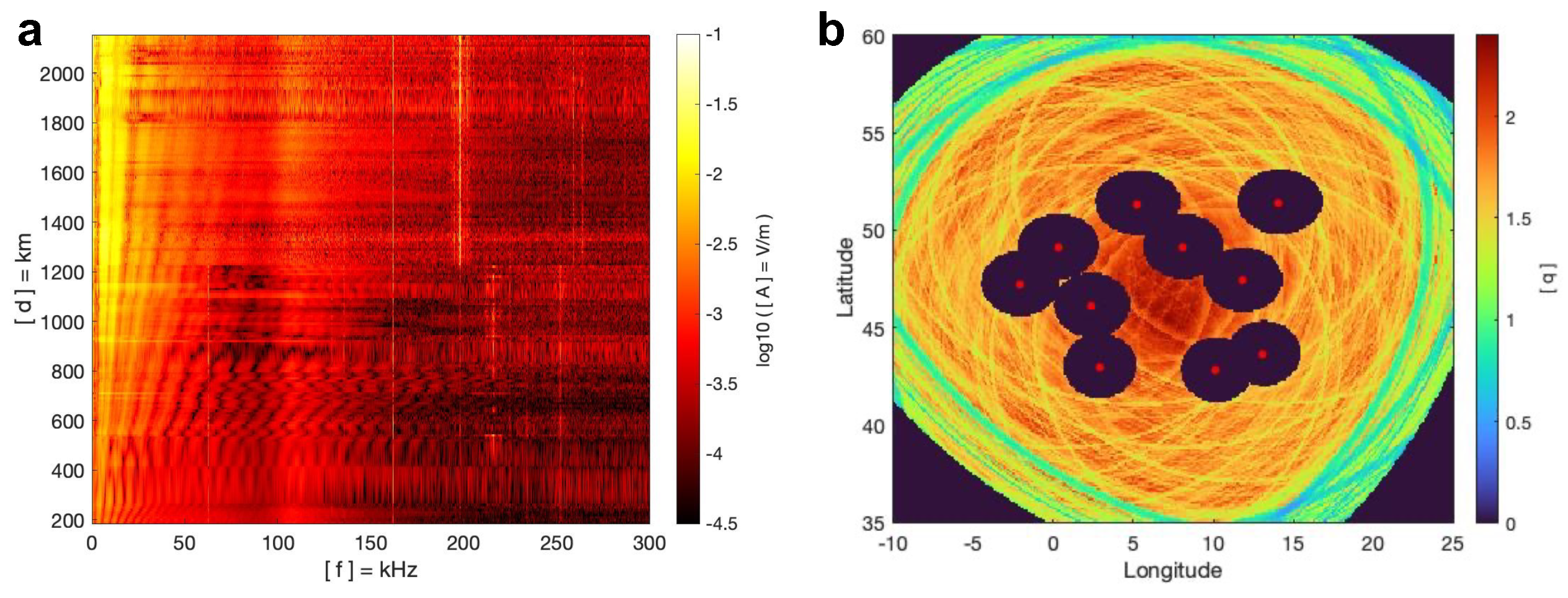
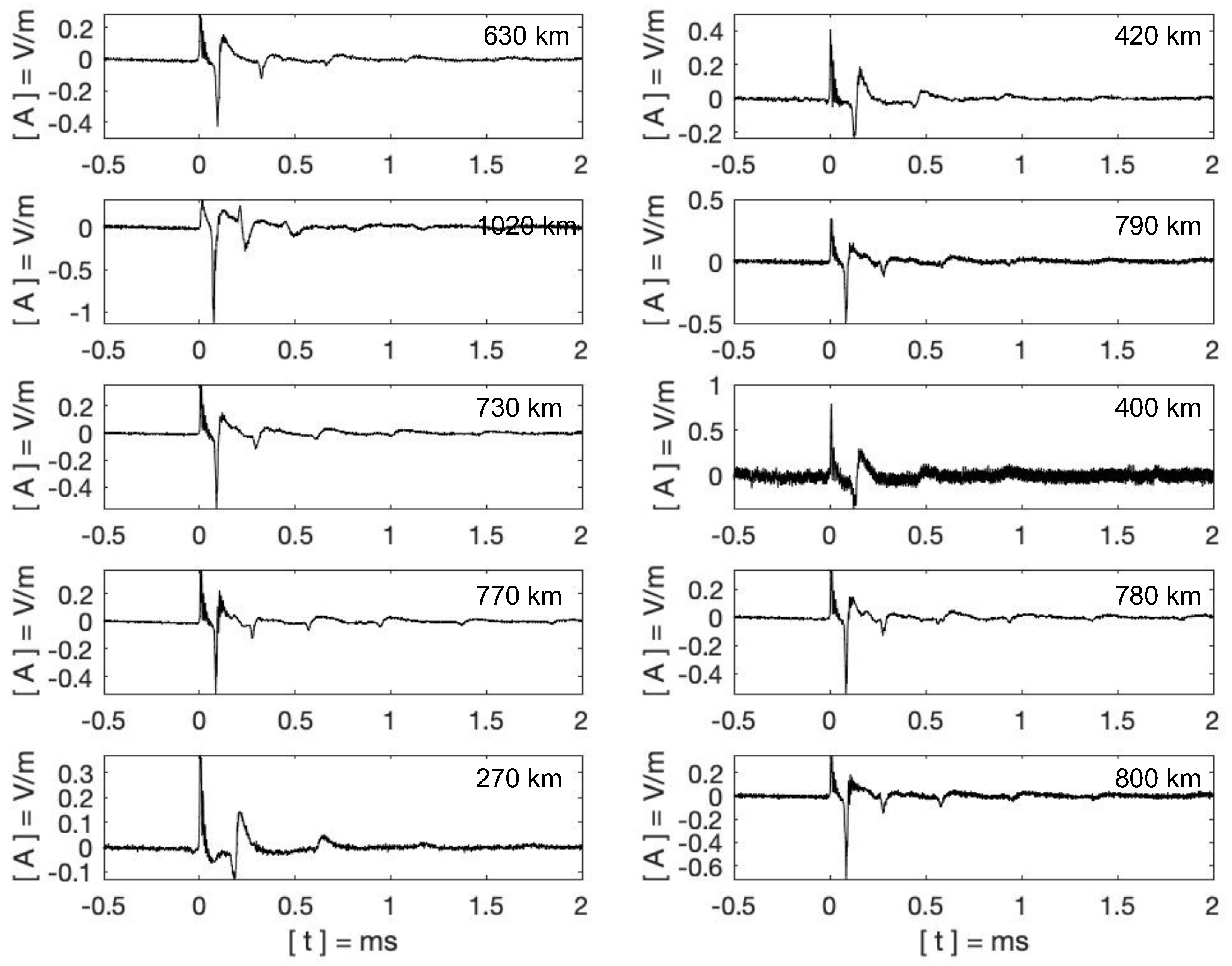
The amplitude waveform bank is calculated based on the sferics recorded by the receivers located in Rustrel and Bath [40,42]. The receiver in Rustrel is selected because this receiver was set up on a remotely located mountain top with a relatively small level of local noise interference. Since most of the lightning events used in this work occurred in France, the waveforms recorded by the receiver in Bath are associated with large propagation distances up to ∼2150 km. The averaged waveforms in the amplitude waveform bank for each distance are calculated by more than 100 events to create a reliable and representative lightning waveform. Therefore, there are some gaps in the waveform bank as a result of the limited number of events for some distances. To fill these gaps in the waveform bank, a linear interpolation is used to calculate a continuous waveform bank (Figure 1a). When calculating the amplitude waveform bank, each lightning waveform is scaled by its ground wave maximum; therefore, the energy of 10 kHz at 2000 km can be larger than at 200 km because this is not the real recorded energy, but rather, the normalised energy. In practice, the ground wave would attenuate largely at 2000 km. However, as this work studies long-distance remote sensing, the waveforms of large distances are kept for subsequent analyses. This figure shows the amplitude waveform bank in the frequency domain.
The waveforms extracted from the amplitude waveform bank in the time domain are referenced to the lightning occurrence time by taking out the propagation time, that is, s. The time point , when considering the timing uncertainty, can be determined by adding a random number based on Equation (3). The coherency for each test pixel is calculated by using Equation (4) and considering the timing uncertainty .
If a distance is outside the distance range covered by the waveform bank, i.e., km or km, the value of this test pixel is set to 0. For each test pixel, the same process is repeated 100 times, and the average coherency of these 100 simulations is used. The quality q is defined in Equation (5) to emphasise the small differences of coherencies [41,45]
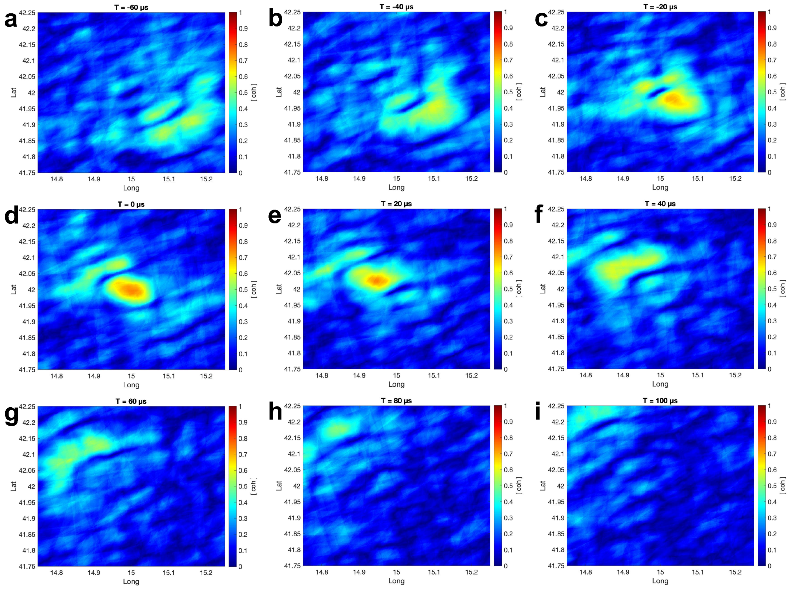
The quality q value for each pixel is shown in the coherency sensitivity map (Figure 1b). The low values around the receiver and at the boundary of the figure are caused by the limited distance range of the amplitude waveform bank. It is evident that the coherency is relatively large, even outside the receiver network. The coherency pattern also depends on the geometric array configuration of the receivers in the network.
3. Coherency
It has been reported by Bai and Füllekrug [42] that the coherency waveform bank can exhibit lightning characteristics with relatively accurate ground wave and skywave arrivals. In that study, coherencies are studied with groups of lightning events which are classified by their propagation distances. In this section, the propagation times are referenced to t = 0 s, which is the lightning occurrence time. After that, all the events will be treated equally despite their propagation distances when calculating the coherency. The only variable that affects the coherency in this section is the case number, i.e., the number of events used to calculate coherency. The purpose of this section is to quantitatively study the lightning and noise coherency, which will be used as a reference when investigating the interferometric method in the following sections.
3.1. Coherency of Lightning Events
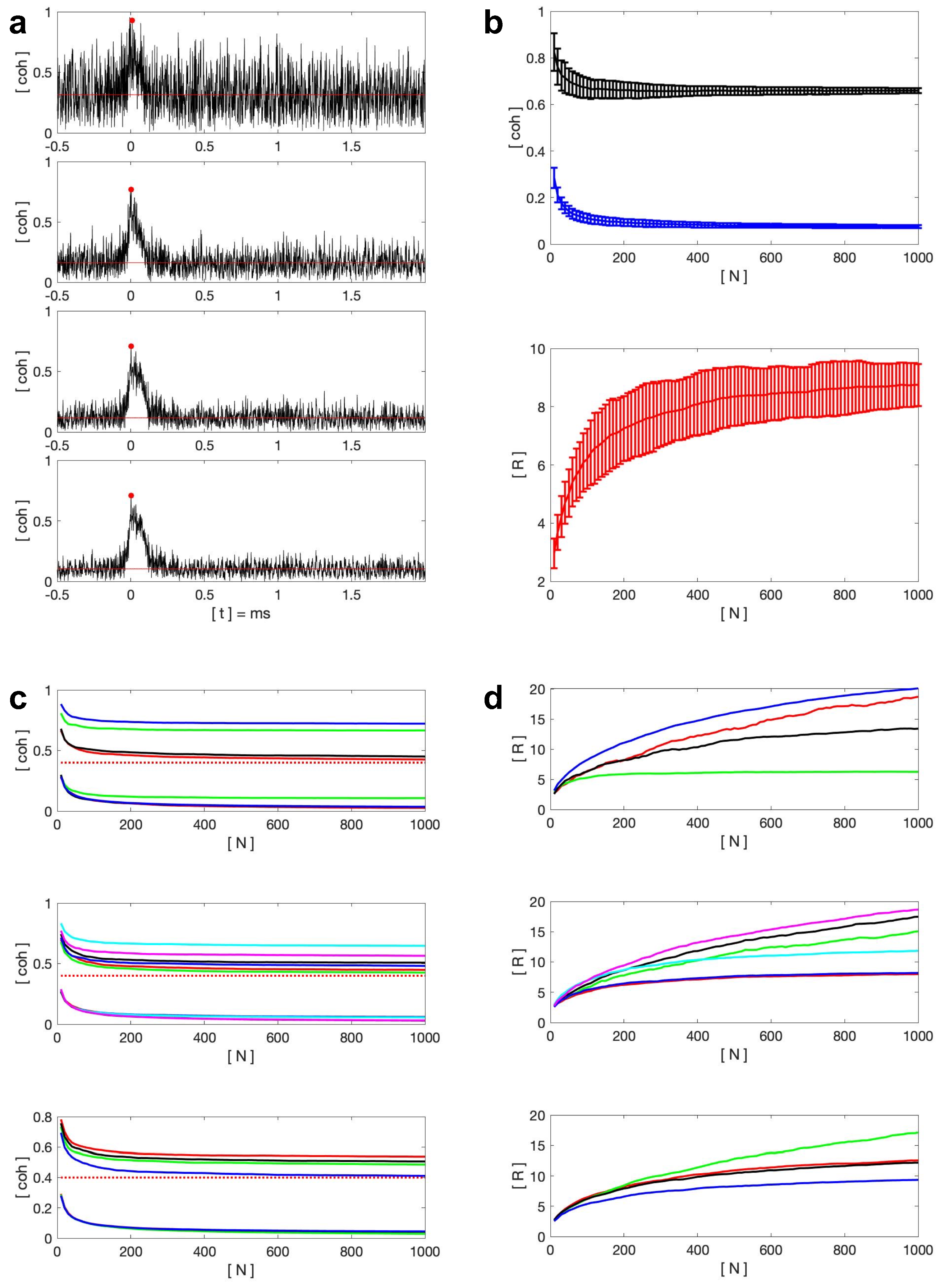
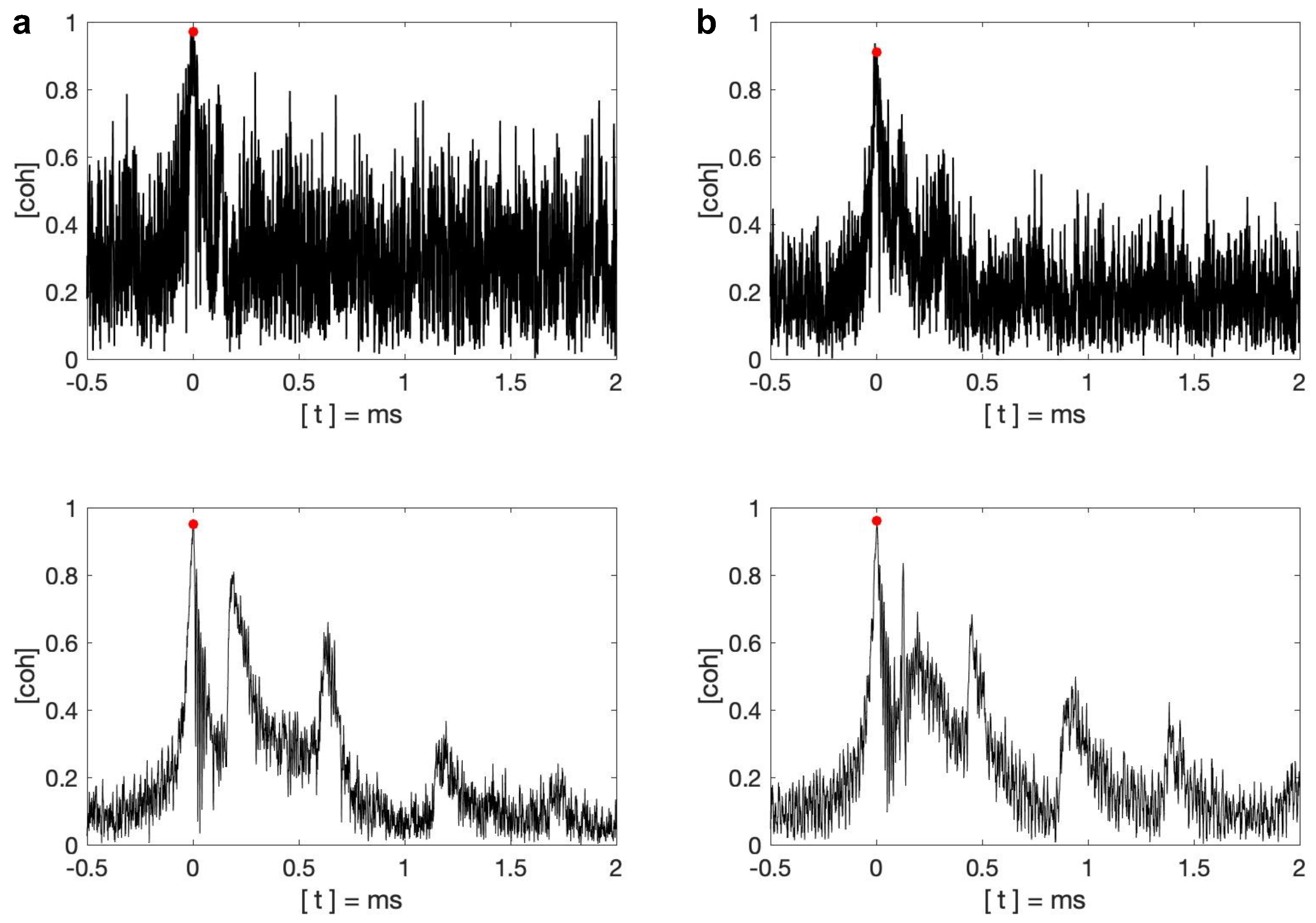
The events used in this section are recorded from four receivers. There are 2000 events randomly selected from each receiver to form an event pool, which has 8000 events in total. The length of each event waveform is 2.5 ms, which ranges from −0.5 ms to 2 ms with respect to the lightning occurrence time. Calculating coherency with different case numbers N can be regarded as calculating the coherency with waveforms recorded from N different receivers of one event. This is different from Section 2, where the receiver number N is 10, the receiver number N, i.e., case number N in this section, is a variable. The coherency waveform is calculated based on N lightning waveforms using Equation (4). The N events are randomly selected from the event pool, which has 8000 events with various propagation distances. The event number N varies from 10 to 1000 in steps of 10 to calculate the coherency based on different case numbers. A step size of 10 is chosen because it still shows a smooth coherence curve, but it does not require as much computation time as using a step size of 1. Here, an example of the calculated coherency waveforms with the event number N of 10, 40, 70, and 100 in one simulation are shown in Figure 2a. For each coherency waveform, the peak coherency associated with the ground wave is marked with the red dot and the threshold coherency is marked with a red line. With the propagation distance increasing, the recorded ground wave will be elongated with a decreased peak. A time window of 0–40 s is used to define the ground wave time range and help find the peak associated with the ground wave. This time window is restricted by the ground wave rise time. The reason why this time window is selected is that lightning events with different propagation distances have different skywave arrival times. Therefore, the time range that is certainly coherent is the time range associated with the lightning ground wave. Long propagation distances will elongate the ground wave rising edge to ∼20 s, and in general, the most accurate phase information is usually present at the ground wave peak. Therefore, to include the ground wave peak, a time window of 0–40 s is used here. Note that the start time of the time window is the lightning occurrence time instead of the ground wave arrival time. The time range outside of this window would be considered as noise, whose mean coherency is defined as the lightning threshold level . The ratio R is defined to help determine a prominent ground wave peak
It can be seen from Figure 2a that, when the event number N is 10, most of the time stamps are highly coherent, and it is hard to distinguish the lightning occurrence time. With increasing event number N, the peak coherency decreases slowly and remains at a high value, while the threshold coherency drops much faster. It means that the coherency waveform with a larger event number N has a lightning ground wave that stands out more with a high signal to noise ratio. Therefore, a large number of receivers recording synchronously at different locations can largely increase the detection accuracy of lightning arrivals in the coherency waveform. When the event number N increases to a threshold value, i.e., ∼100, the peak coherency and the threshold coherency tend to be stable at 0.51 (±0.005) and 0.08 (±0.008), respectively (Figure 2b). In this example, the skywave is not distinguishable because the events used to calculate the coherency waveform have different propagation distances. Therefore, the skywave arrival times are different and not coherent with each other.
This process has been run 100 times to increase the reliability of the results. There are three evaluation factors: threshold coherency , peak coherency , and ratio R are recorded based on the event number N. The mean value and the standard derivation of each evaluation factor are calculated and shown in Figure 2b. It can be seen that with increasing event number N, both and decrease at a different rate. The ratio R increases with the event number N, which has a logarithmic growth. It is worth mentioning that, contrary to expectations, the peak coherence usually occurs between 0 and 5 s, which is near the lightning occurrence time. As mentioned earlier, according to different propagation distances, the rising edge of the ground wave has different time ranges, which means that the peak of the ground wave arrives at different times. Therefore, for different lightning events with different ground wave peak times, the lightning occurrence time, that is, t = 0 s, is relatively consistent, so it has the largest coherency.
This study quantitatively investigates the practical coherency of lightning events based on the event number N, which will be compared with the noise coherency in Section 3.3 and used as a reference in Section 4, Section 5 and Section 6.
3.2. Coherency Analysis over Lightning Event with Different Selections of Receiver Locations
In the last section, the event pool consists of the events of four locations. To analyse the location performance, the same simulations are repeated with different event pool compositions. This section aims to evaluate location performance and provide statistical support for location selection in the following interferometric method study.
The coherency results based on different selections of locations are shown in Figure 2c,d. Figure 2c shows the threshold coherency and the peak coherency , while the curves with a value above 0.4 are associated with the peak coherency.
As for the threshold coherency, the single receiver result shows that the receiver in Toulouse has the highest threshold coherency, while the other three receivers share the same threshold coherency. It indicates that other electromagnetic field sources in Toulouse can interfere with the recordings when monitoring the lightning activity. This conclusion is corroborated by analysing the results of two locations and three locations. In the two locations figure, the threshold coherency calculated from the receiver pairs Bath and Toulouse, Orleans and Toulouse, and Rustrel and Toulouse is comparable and slightly higher than the other three location pairs, that is Bath and Orleans, Bath and Rustrel, and Orleans and Rustrel. This shows that as long as the receiver in Toulouse is involved with event selection, the threshold coherency will be relatively high. And the results of three locations show that the receiver group including the receivers in Bath, Orleans and Rustrel produce a minimum threshold coherency . It means that the receiver selection without the receiver in Toulouse can produce a relatively low threshold coherency.
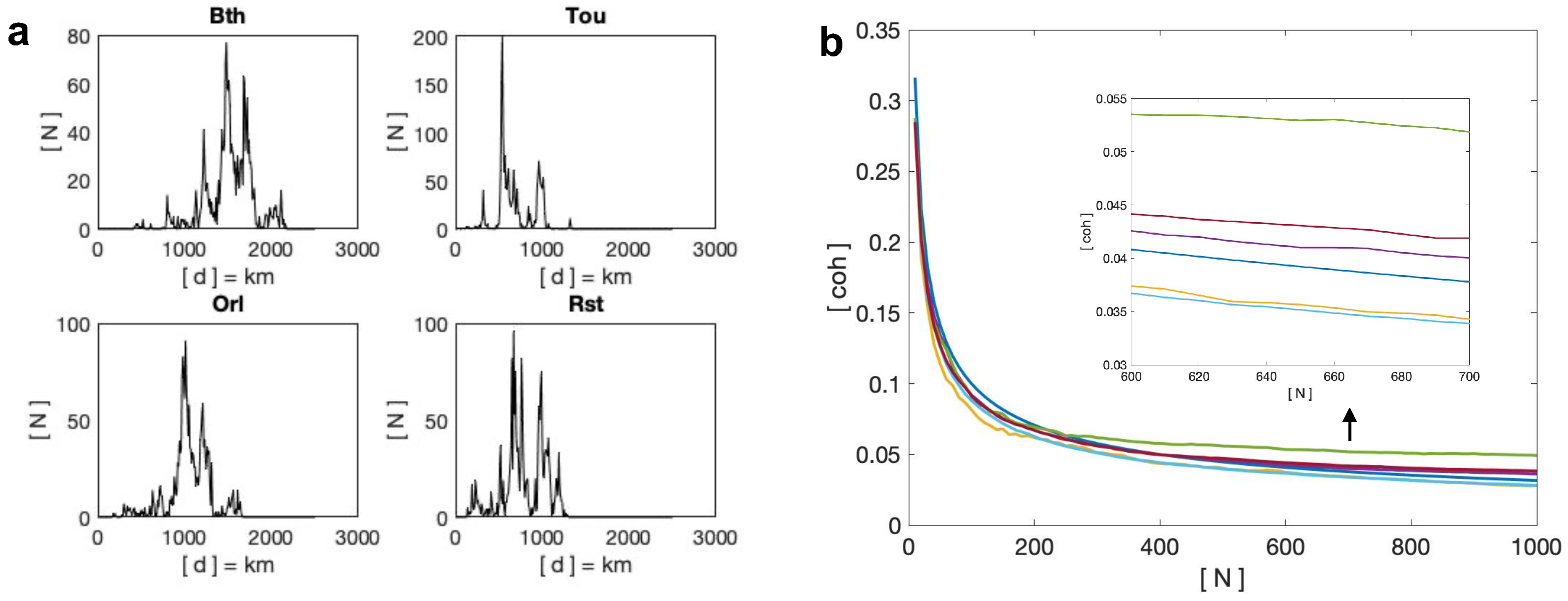
The same analysis procedure is carried out for peak coherency . It can be concluded that the peak coherency > > > by analysing results produced by different selections of locations. To gain more information on these simulated events, the event distance distribution is plotted based on the receiver location in Figure 3a. Therefore, the possible reasons that caused different peak coherency can be (1) the events used in this section happened in Southern France, which leads to larger propagation distances of the recorded waveforms in Bath and causes a minimum coherency peak value; (2) to quantitatively analyse the distance distribution, the mean distance to Rustrel is similar to Toulouse, which is smaller than the mean distance to Orleans, and Bath has the maximum mean distance. It is suggested by Bai and Füllekrug [42] that the large distance can lead to a lower ground wave coherency; (3) the receiver in Rustrel was remotely located on a mountain top with the minimum noise level. In addition, the waveforms recorded in Rustrel have a better quality, i.e., larger signal to noise ratio, compared to the waveforms recorded in Toulouse, which can produce a larger peak coherency.
The results calculated with the receiver in Toulouse have both high levels of threshold coherency and peak coherency may indicate this location is better at recording electromagnetic fields. To find out which location is better at detecting lightning signals, the ratio R is a more practical evaluation factor. From all three sub-figures, it can be seen that the ratio R values are comparable when event number N is 10. With event number increasing, the ratio > ≈ > . It means Rustrel is the best location in this study for monitoring lightning, while Toulouse is the worst location among these four locations. However, even the coherency calculated based on the events recorded in Toulouse has a ratio R of 2.9 when the event number is 10 and can reach ∼5 when the event number is larger than 100.
3.3. Coherency of Noise
The coherency noise level depends on the event number N; that is, the theoretical noise coherency scales with ∼1/. In this section, the coherency is calculated based on recorded noise with the theoretical value ∼1/ as a reference. This section provides the experimental basis for the selection of data sources when testing the interferometric method in the following sections.
The coherency of the recorded noise is evaluated based on the receiver location. The noise is defined as the electromagnetic field recordings when there is no lightning activity within the distance range of 1000 km. For each location, more than 4000 noise waveforms are selected, and each noise waveform has a time length of 2.5 ms to be consistent with the analysis of lightning signals in the previous sections. Since the lightning events used in this work were all recorded during the night time, the noise waveforms were also selected from the measurements during the night time as explained below. However, there were active lightning storms during each recording date, so it is hard to find a time long enough to have the number of noise waveforms meet the overall search criteria. Therefore, the noise waveforms are extracted during the time between lightning events. To make sure each noise waveform does not include any lightning activity, the time gap between the occurrence time of two lightning events, which are used to extract the noise waveform, needs to be longer than 2 s. The noise waveform start time is 1 s after the occurrence time of the first lightning event. For each qualified time gap, only one noise waveform is selected because there are meaningful background signals in the Toulouse and Orleans recordings. If continuous recordings are taken, they would be coherent. This step is to break the continuity of the phase information that exists in periodic signals. The frequency components below 1 kHz are filtered out using a digital filter because in this frequency range, some meaningful signals lead to highly coherent phase information. The source of this coherent signal is the power line harmonic radiation.
The coherency of noise waveforms is evaluated with different event numbers N, and the mean values of recorded noise coherency for each station are plotted in Figure 3b. When the event number N is 10, the coherency of the noise recorded from four locations all starts from ∼0.28. As the event number increases, the recorded noise coherency starts to decrease and the differences between the four locations start to be clear. The recorded noise coherency in Orleans has the maximum value, while the recorded noise coherency in Bath and Rustrel exhibit a smaller value. The low coherency of the recorded noise means during a quiet time (when there is no lightning activity), the local background does not have many meaningful sources (coherent signals) and is preferred to be used as a location for lightning recording.
Figure 3b shows the coherency of the following three categories: recorded noise, theoretical coherency ∼1/, and the lightning event threshold coherency . It can be seen that for various event numbers N, the recorded noise coherency follows the simulated noise coherency and matches with the theoretical noise coherency. It is worth mentioning that the lightning event threshold coherency also follows the noise coherency, which means except for the ground wave, the other time range is not coherent and can be regarded as noise. This analysis offers a reference to the coherency of noise, based on the event number N, which will be used in the following study of interferometry in the next section.
4. Interferometric Method with Averaged Waveform
The existing lightning detection and location networks commonly use the Time-of-arrival (TOA) technique, which only selects a single time stamp from each recorded lightning waveform. This selected time stamp is usually the start of the rise time, zero crossing time, or maximum electric field time. The zero-crossing time is determined by the maximum electric field, that is, using the 10% and 90% of maximum electric field points to define a line, and the zero-cross time is when this line crosses zero. The TOA technique is simple to use and has high accuracy. However, to expand the use of recorded waveforms and explore the information possibly contained in the received waveforms, the interferometry method is introduced here.
The idea of the complex interferometric method is to use coherency to simulate interferometric lightning location by mapping the lightning event into an area rather than a single location. In this map, each pixel corresponds to a lightning location with a different time of arrival difference, and the coherency is shown for each pixel. These time of arrival differences are simulated by shifting the lightning waveforms.
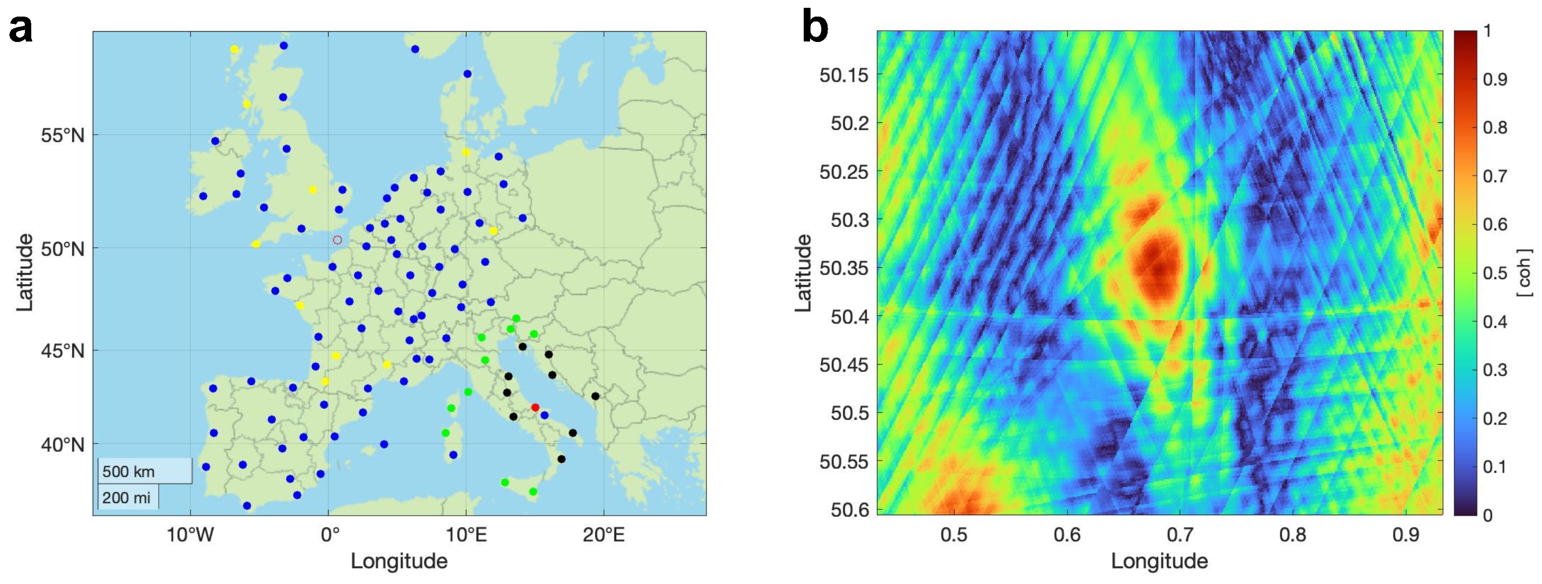
The real lightning receiver locations in Europe are used for simulations to be more realistic (Figure 4a). To investigate this method, the averaged waveforms from the amplitude waveform bank are first used here to create the best possible result. It is worth mentioning that the amplitude waveform bank used here is only based on the data collected in Bath and Rustrel because (1) enough data are collected during the campaign and the data collected in these two locations are enough for this study; (2) the noise coherency study in Section 3.3 shows that the data collected from Bath and Rustrel have a relatively large signal to noise ratio; (3) the study in this section requires a large distance range because the receiver network used here covers a large area of Europe and only the data collected in Bath can cover that large distance range.
In this work, the lightning events are simulated at different locations with all European receivers. The European receivers cover a large area which would require long-distance events, while the Rustrel data can only cover a distance up to 1340 km and Bath data can cover a distance up to 2150 km.
In addition, N receiver locations (yellow dots in Figure 4a) are specifically selected to be evenly distributed around the simulated lightning location L (red circle). The distance between the simulated lightning location L and the selected receiver location can be calculated to extract the corresponding waveform from the amplitude waveform bank. From Figure 2d, it can be seen that with the number of 10, which refers to a lightning detection and location network with 10 receivers, the ratio R between the peak coherency and the threshold coherency is ∼2.6. It means a coherency map based on 10 receivers can exhibit a good contrast between the ground wave and the background noise. A coherency map example is shown in Figure 4b to help explain this interferometric methodology. The selected averaged waveforms from the amplitude waveform bank are shown in Figure 5.
The simulated lightning location L is put at the centre of the coherency map in Figure 4b. The time for this coherency map is set as 0, which is the occurrence of the selected waveforms. The occurrence time is chosen because in the simulations in Section 3.3, it is found that peak coherency typically occurs between 0 and 5 s. Therefore, the coherency of the pixel L is the coherency calculated based on the time in 10 averaged waveforms
where is the averaged waveform refers to n-th receiver.
The coherency of other pixels P depends on the relative distance towards the simulated lightning location L, and the coherency needs to be calculated by shifting the selected averaged waveforms. The distance difference between the test pixel P to n-th receiver location and the lightning location L to n-th receiver is
where is the distance between the test pixel P and n-th receiver, and is the distance between the simulated lightning location L and n-th receiver.
The time delay of the test pixel P compared to the simulated lightning location L for n-th receiver is
under the assumption that lightning propagation velocity equals the speed of light. The coherency for the test pixel P is
This method uses much more information about a lightning waveform compared to the traditional method, which only picks a single time stamp for each event, and can give an uncertainty of lightning location information of a single event.
5. Interferometric Method with Whole Receiver Network
In the last section, the interferometric method is investigated using the averaged waveforms from the amplitude waveform bank. In this section, the waveforms of individual events are used. Coherency and amplitude values are studied separately to be shown in each pixel in the map. To expand on the results, time can be varied to refer to different times. A collection of maps with different times is defined as a dynamic map, which shows the movement of the apparent lightning location inferred from the coherency.
5.1. Coherency Map
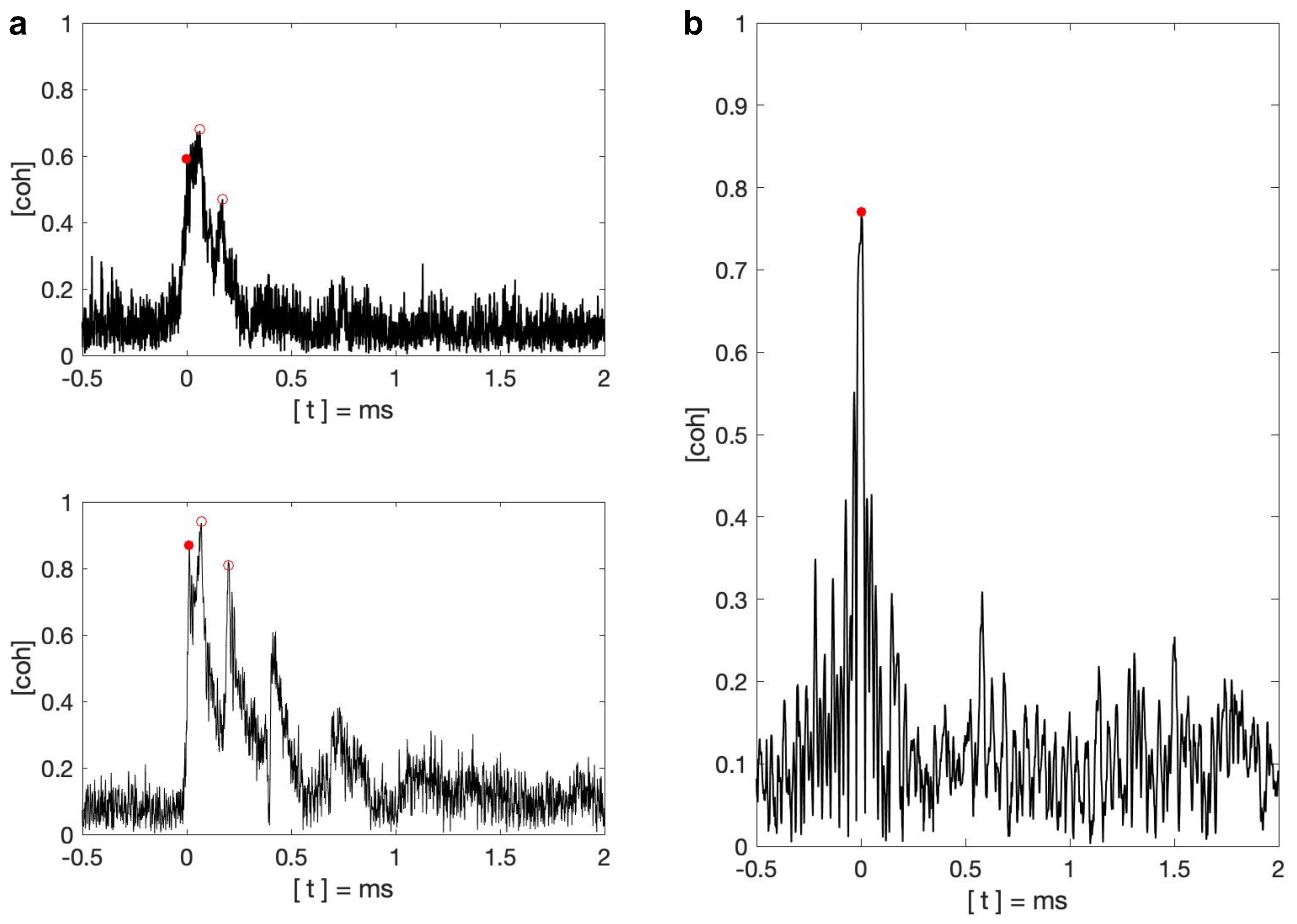
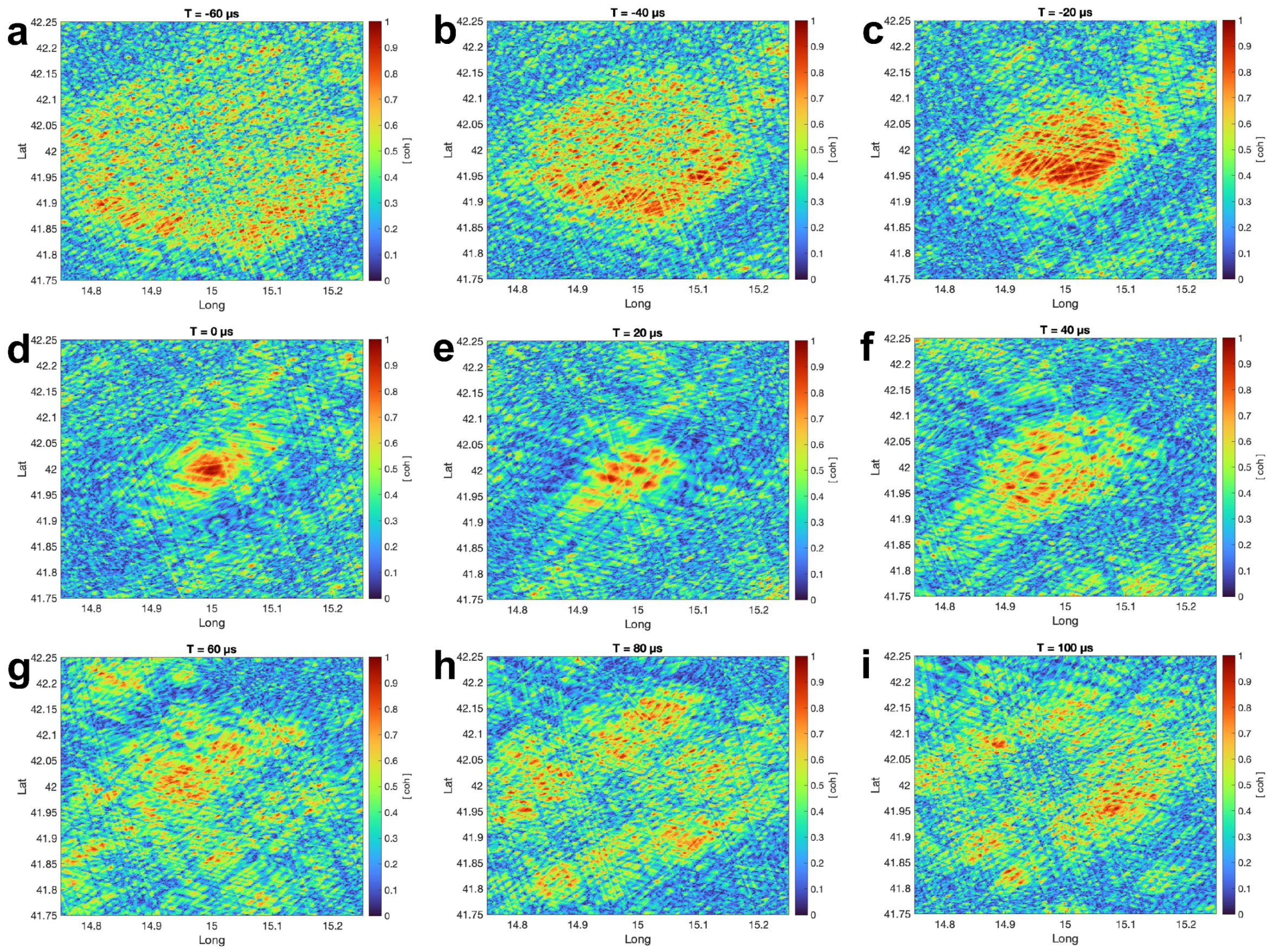
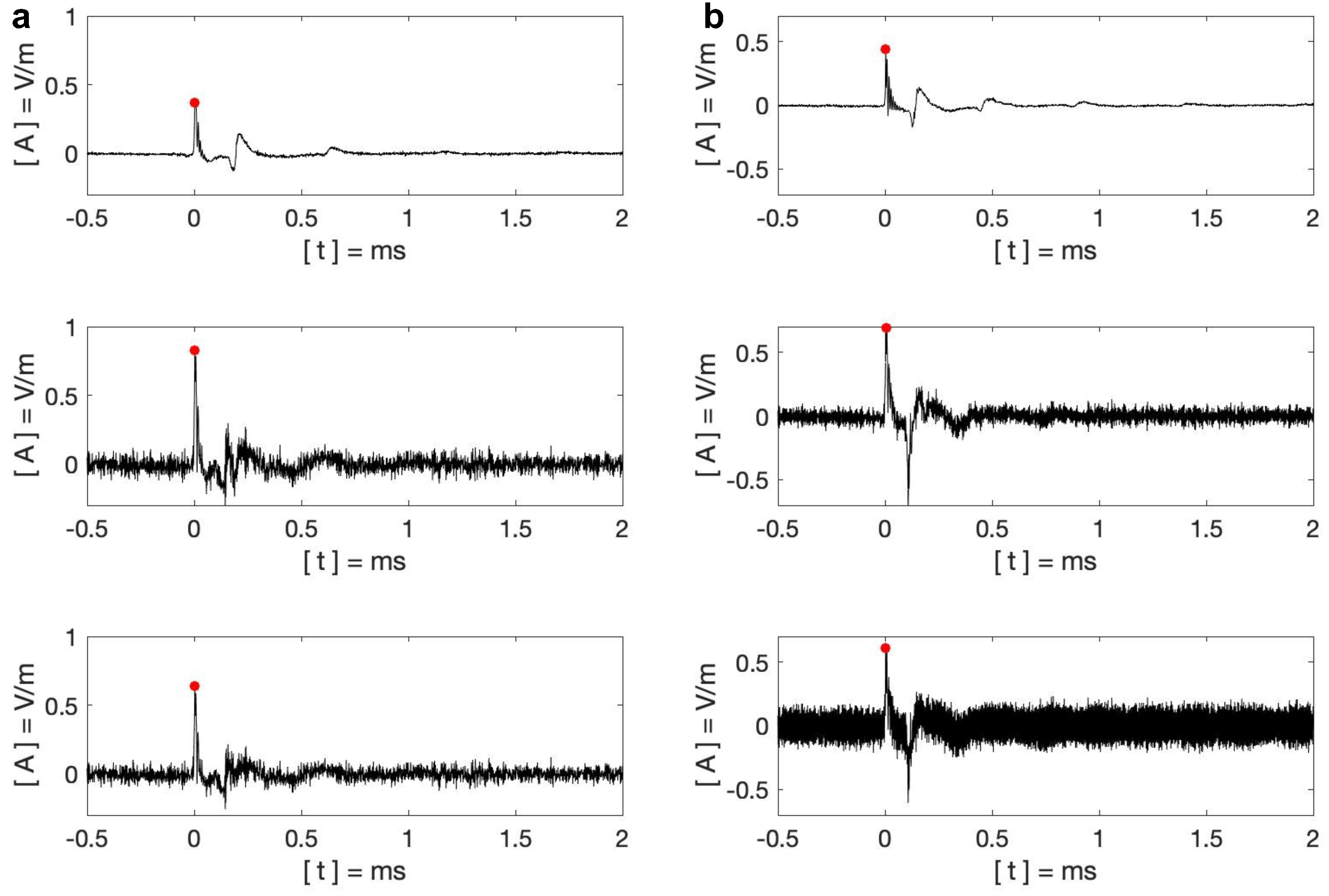
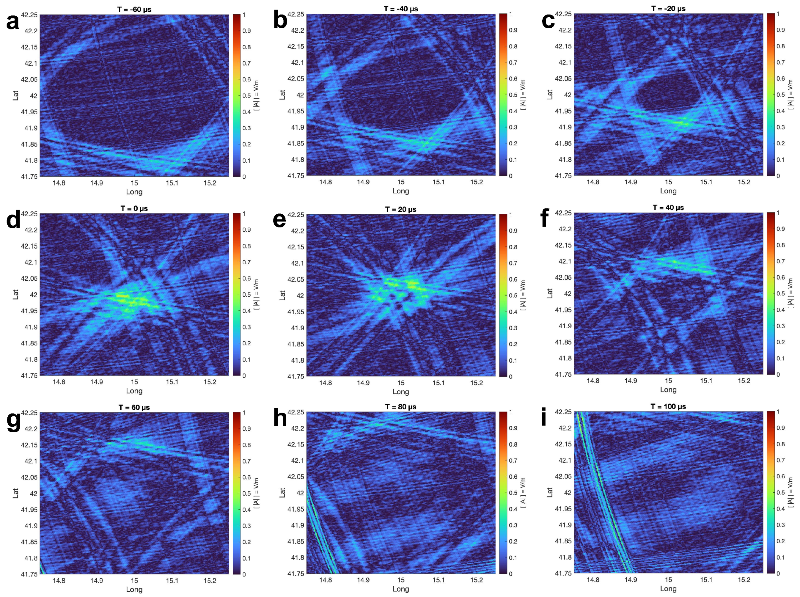
The coherency map performance depends on the receiver number; all 105 available receiver locations are used for the simulation to illustrate a dynamic coherency map. The simulated lightning location L is put at different locations to investigate the effects of relative positions of lightning location and lightning detection network. Ten different lightning locations are simulated, and an example is shown in this section for illustration. This simulated lightning location has a longitude and latitude of 15°E and 42°S, which is located at the South–East part inside of the receiver network (Figure 4a). The start and end times of are −60 s and 160 s with a step time of 20 s. In addition, the waveform used here is not the averaged waveform from the amplitude waveform bank. Instead, waveforms of individual events are used. The distance is the distance between the simulated lightning location L and n-th receiver. From all the events recorded at Bath and Rustrel, the event with the closest propagation distance to distance is selected to represent the recordings of n-th receiver. The coherency waveform calculated based on is shown in the upper figure in Figure 6a. The average propagation distance of these selected waveforms is ∼1149 km; therefore, the coherency waveform of 1150 km from the coherency waveform bank is shown in the bottom Figure 6a for comparison.
The coherency waveform calculated by the selected individual events shows that the coherency reaches the local maximum and global maximum values of 0.59 and 0.68 at 0 s and 62 s, respectively. The coherency of the coherency waveform of 1,150 km reaches the local maximum and global maximum values of 0.87 and 0.94 at 12 s and 69 s, respectively. Both local maxima are associated with the ground wave, and global maxima are associated with the 1st skywave. The local maximum values associated with the 2nd skywave are 0.47 at 171 s and 0.81 at 201 s for the calculated coherency waveform and coherency waveform from the coherency waveform bank, respectively. This shows that a mixture of different propagation distances can produce a less coherent waveform but has fewer effects on the arrival time of skywaves. According to the receiver distribution map in Figure 4a, even though they have various locations, the majority share similar propagation distances, which are close to 1150 km. It explains the small amount of timing changes. Another reason that the calculated coherency waveform has lower maximum values is that the coherency waveform bank only uses the data collected in Rustrel. From Figure 2c, it can be seen that the Rustrel data has a larger coherency peak value than the data collected in Bath. It is worth mentioning that the peak coherency calculated based on data collected with the location pair Bath–Rustrel is ∼0.55 with an event number of 100 in the middle figure of Figure 2c. This value matches well with the local maximum value associated with the ground wave in the calculated coherency waveform.
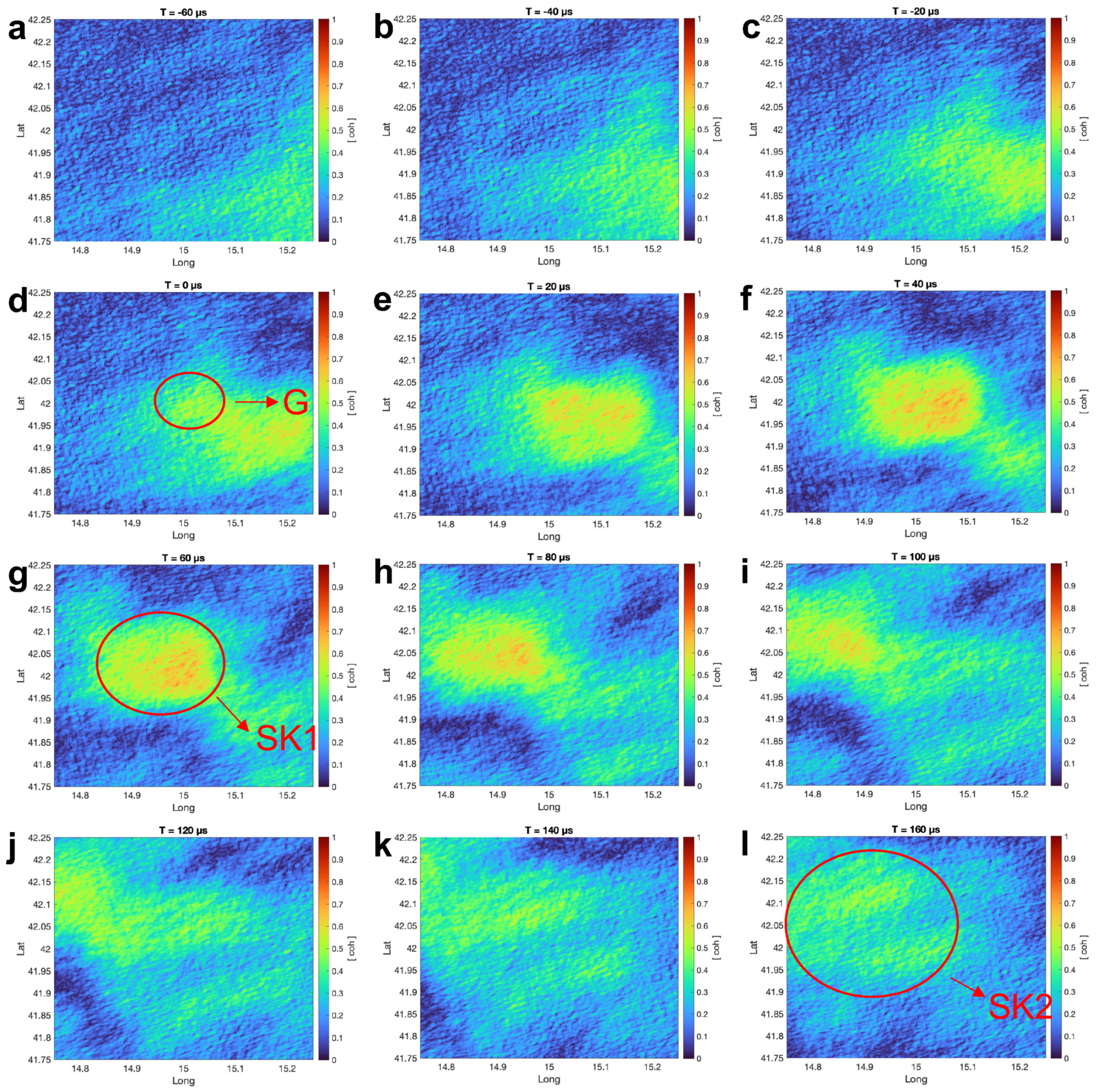
Figure 7 shows that the front of the ground wave arrives at the simulated lightning location at −20 s while the centre of the ground wave reaches the simulated lightning location (the centre of the image) at 0 s. Right after the ground wave is the first skywave, which covers a larger area and a higher coherency. The centre of the 1st skywave reaches the simulated lightning location with a maximum value of ∼0.7 in the time frame of 60 s. The second skywave arrives at the simulated lightning location closely after the first skywave. It covers an even larger area with a lower coherency at ∼0.5 at the time frame of 160 s. The arrival times of the ground wave and the first two skywaves in the dynamic coherency maps coincide with the time reflected in the calculated coherency waveform. The background noise value is ∼0.1, and it matches well with the simulated noise coherency in Section 3.3.
5.2. Amplitude Map
In this section, the interferometric method is used to produce amplitude maps. When coherency is calculated, the energy of an individual event does not need to be considered as the coherency calculation only involves the phase information. However, the amplitude is strongly related to the event peak current. When producing the amplitude map, the impact of event energy intensity needs to be mitigated. The concept of relative amplitude is introduced here using two methods. The first method is normalising the amplitude waveform by its local maximum electric field associated with the ground wave. This normalised amplitude waveform is called the scaled amplitude waveform, and the corresponding amplitude map would be called the scaled amplitude map. The second method uses the experimental attenuation coefficient introduced in [42,46,47] to determine the calculated peak current based on the local maximum electric field associated with the ground wave. Then, the amplitude waveform is scaled by the ratio , which is defined as the ratio between the calculated peak current and the peak current reported by Méteorage. The corresponding relative amplitude waveform is called the ratioed waveform, and the amplitude map derived by the ratioed waveform would be called the peak current map.
Similar to the coherency map, when calculating the amplitude map, the amplitude value of the pixel refers to the simulated lightning location L that needs to be calculated first. The absolute amplitude value is used here, which is
where is the amplitude waveform recorded at receiver. With the same definition of in Equation (9), the amplitude value for the simulated pixel P is
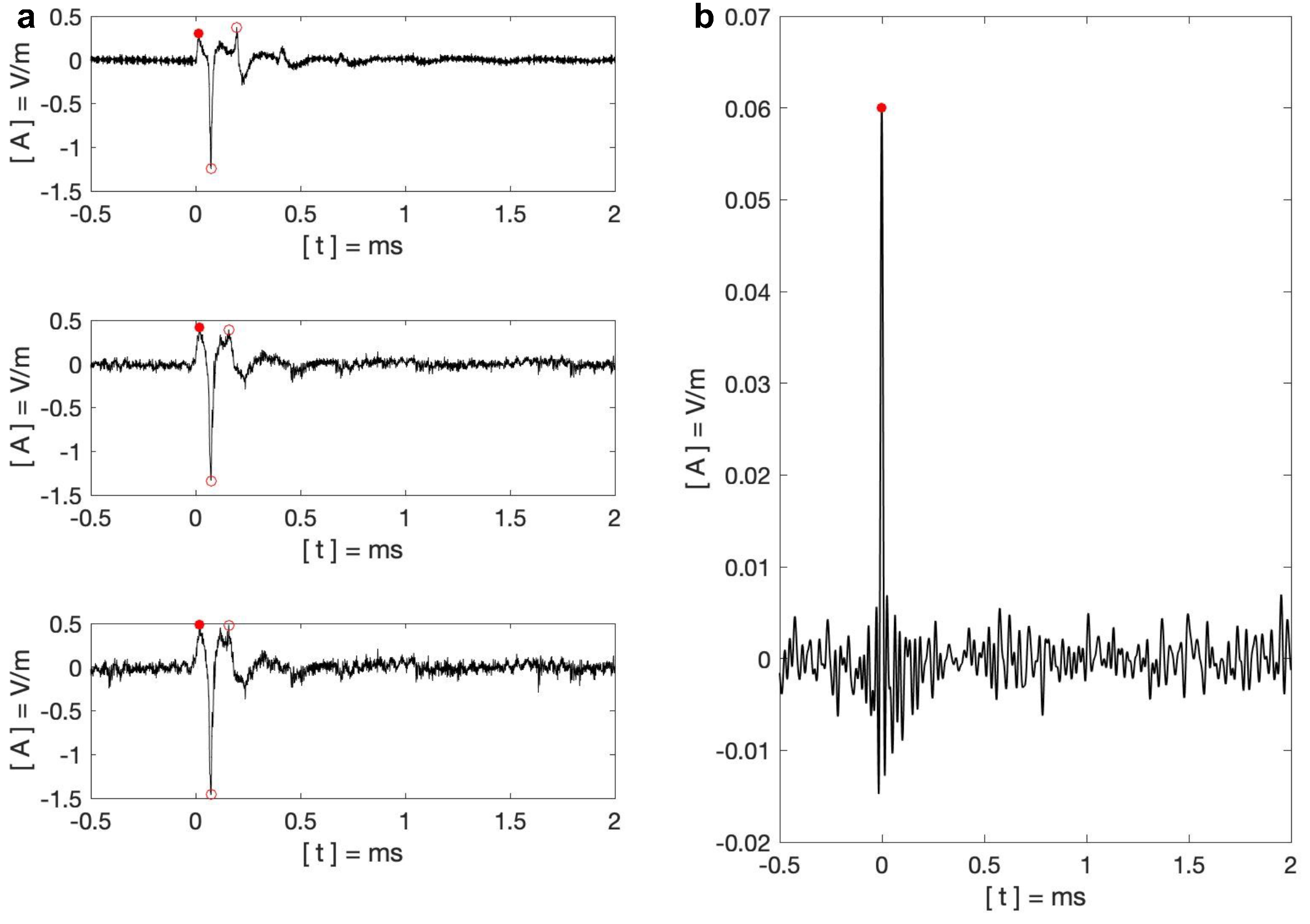
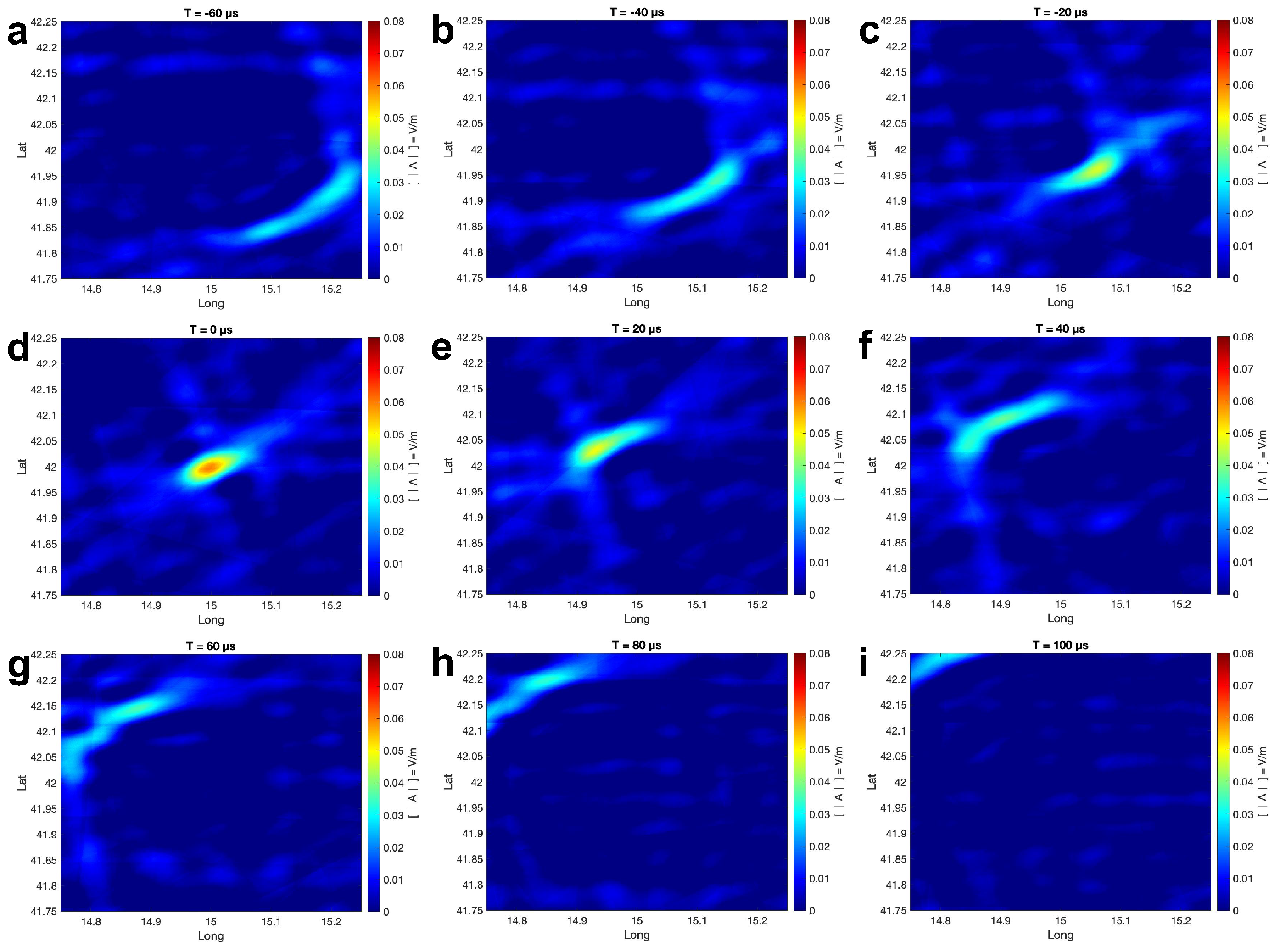
For comparison with the coherency map, the amplitude map examples use the same simulated lightning location, whose longitude and latitude are 15°E and 42°S. The averaged waveform of 1150 km from the amplitude waveform bank is shown in the upper figure of Figure 8a. The ground wave reaches the maximum value of 0.30 at 14 s. The first skywave and second skywave reach the absolute peak values at 73 s and 196 s at −1.24 and 0.37, respectively.
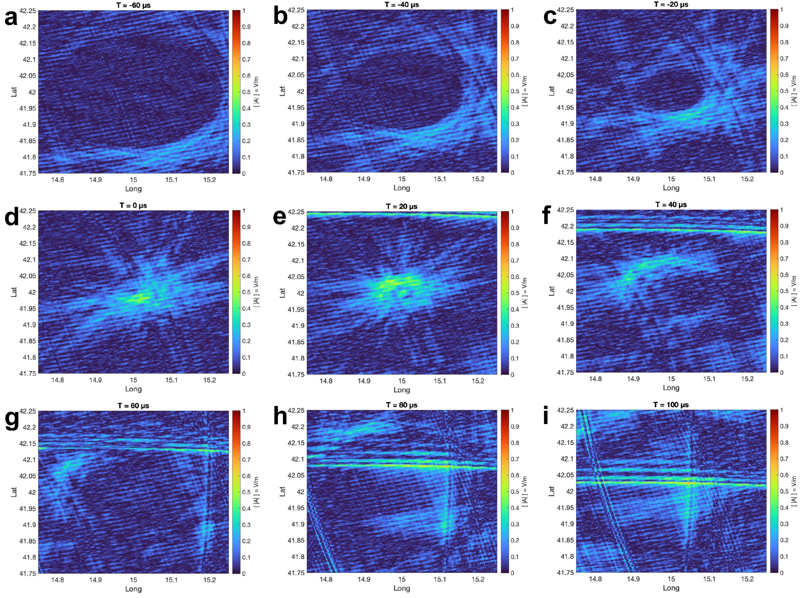
The amplitude map using the scaled amplitude waveform is shown in Figure 9, where the preset lightning location is located at the centre of the image. The calculated scaled amplitude waveform is shown in the middle figure in Figure 8a. It can be seen that the local maximum associated with the ground wave has a value of 0.42 at 17 s. The global absolute maximum value is associated with the first skywave, which has a value of −1.34 at 74 s. The local maximum associated with the second skywave has a value of 0.39 at 158 s. The initial prediction of the ground wave value of the scaled amplitude waveform is 1 because each event waveform is scaled to the ground wave maximum. However, the ground waves of different events are elongated based on their different propagation distances. Therefore, the selected events do not reach their ground wave maxima at the same time, and the ground wave in the scaled amplitude waveform is the result of the cancellation of the individual waveform values, resulting in a lower ground wave value. The arrival times of the ground wave and the first skywave of the scaled amplitude waveform match well with the amplitude waveform of 1150 km from the amplitude waveform bank.
Figure 9 shows the apparent lightning energy movement. Since the global absolute maximum value is 1.34, the colour scale limit of the scaled amplitude map is set to 0–1.5 considering the waveform value cancelling. Compared to the first skywave, the area associated with the ground wave has a much smaller value in scaled amplitude maps. The ground wave has a comparable value to the second skywave, while the second skywave covers a larger area. The first skywave is predominant in the dynamic amplitude maps. To quantitatively analyse the amplitude maps, the ground wave arrives at the simulated lightning location in the time frame of 20 s, with a value of ∼0.4. Then, the first skywave starts to move towards the simulated lightning location and reaches the centre between the time frame 60 s and 80 s. The maximum value in these two frames is ∼1.3. The second skywave arrives at the simulated lightning location in the time frame of 160 s with a value of ∼0.4. The results of the dynamic amplitude maps match with the analysis of the scaled amplitude waveform in Figure 8a.
The ratioed amplitude waveform is shown in the bottom figure of Figure 8a. The local maximum associated with the ground wave has a value of 0.49 at 17 s. The peak associated with the first skywave has a value of −1.46 at 73 s. The peak associated with the second skywave is at 158 s with the same value of 0.48.
As the peak current maps exhibit similar results as the scaled amplitude map, the peak current maps are not shown here. The ground wave arrives at the simulated lightning location in the time frame of 20 s with a value of ∼0.5. The first skywave reached the simulated lightning location between the time frame of 60 s and 80 s, with a maximum value of ∼1.5. The second skywave covers a large area and it reaches the simulated lightning location in the time frame of 160 s. Similar to the scaled amplitude maps, the peak current maps exhibit a predominant first skywave and less significant ground wave and second skywave.
The interferometric method using the amplitude shows similar results even with different definitions of relative amplitude waveform. When comparing the amplitude map with the coherency map, there are some conclusions that can be drawn: (1) both methods show clear boundaries between the ground wave, first skywave, and second skywave; (2) the ground wave reaches the simulated lightning location at 0 s and 20 s in coherency maps and amplitude maps, respectively; (3) coherency maps exhibit a comparable value of ground wave and first skywave, while the amplitude maps have a predominant first skywave and less significant ground wave and second skywave. This means that it is hard to identify the ground wave presence with the large first skywave value in the amplitude maps; (4) the coherency maps have larger signal to noise ratios for the ground wave such that the contrast between the lightning event and the background noise is obvious, while the amplitude maps have lower signal to noise ratios; (5) both methods have the same apparent movement direction.
5.3. Apparent Lightning Movement
To investigate the possible cause for the apparent lightning energy movements in both the amplitude maps and coherency maps, different lightning locations are simulated. The results show that the movement directions are associated with the relative locations of the simulated lightning locations and the lightning receiver network. The maximum coherency and average amplitude of all the simulated lightning events exhibit apparent movements toward the centre of the lightning receiver network.
This movement can be explained by the waveforms used to simulate the interferometric method. The simulated lightning location of 15°E and 42°S is taken to explain this particular feature, which only exists in the long-range interferometric method and is inevitable. According to Figure 4a, there is a large number of receivers sharing similar propagation distances for this simulated event. It means that not only would the phase of the ground wave be coherent, but the first skywave phase would also be highly coherent. This leads to the large coherency for both the ground wave and the first skywave in the upper figure of Figure 6a. Due to the long propagation distance, the time delay between the ground wave and the first skywave is small, which makes the ground wave and first skywave merge into one wide pulse. According to the definition of the coherency in Equation (10), for different pixels at different time frames , the maximum coherency can only be achieved by the pixel of the simulated lightning event at the time where the coherency waveform in the upper figure of Figure 6a reaches to the maximum value. Therefore, in this example, the coherency reaches the maximum value in the time frame = 60 s, which is associated with the first skywave. Instead of distinguishing the ground wave and first skywave in this example, the phase of the selected waveforms in the time range 0–75 s is highly coherent, and this time range is treated as a wide lightning pulse. For the time frame before = 60 s, the pixels with large coherency require large values of . The large means large , which means the pixels with large coherency are further away from the receiver group than the simulated lightning pixel. In this example, the pixels further from the receiver than the simulated pixel are the pixels located southeast of the lightning pixel. Similarly, for the time frame after s, the pixels with large coherency are closer to the receiver group than the simulated lightning pixel, which are the pixels located northwest of the lightning pixel in this example. Therefore, the direction of the lightning movement is from southeast to northwest—in other words, from the area further from the receiver group towards the receiver group.
In the LF long-range interferometric method, the time range with high energy is quite long because both the wide ground wave pulse and the first skywave can merge into the ground wave with its large value. As long as the lightning pulse has a width, the apparent lightning movement can not be eliminated. However, the lightning location can still be determined by finding the pixel with the maximum coherency/amplitude value. To have a clear peak coherency that is only associated with the ground wave, there are two methods used to remove the first skywave interference: (1) use a small network where the recorded waveforms have small propagation distances. This method naturally decreases the first skywave value and enlarges the time delay between the ground wave and the first skywave. Therefore, the time associated with the first skywave would not be involved in the process of calculating the coherency maps or amplitude maps. This method will be introduced in Section 6; (2) use an impulse to represent the recorded lightning event and calculate the coherency and amplitude map based on impulses. This method will be described in Section 7.
6. Interferometric Method in Small Receiver Network
In this section, small receiver networks are simulated. A small network means smaller propagation distances between the lightning location and each receiver. Therefore, the recorded waveforms have more distinguishable ground waves because: (1) ground waves receive fewer attenuation effects from Earth curvature (2) the time delay between the ground wave and the first skywave is larger. In addition, as there are fewer receivers are needed in a small network, the receivers are selected to distribute around the simulated event. Therefore, there will be no apparent lightning movement effects as the simulated lightning event locates at the approximate receiver network centre.
To have a consistent comparison with previous sections, the simulated lightning event locates at 15°E, 42°S. Two small receiver networks are simulated in Figure 4a with N = 10 and N = 20.
For the 10 receiver network example, 10 events are selected with the closest propagation distances. The average propagation distance of these 10 events is 273 km. Therefore, the coherency waveform of 270 km from the coherency waveform bank is shown in the bottom figure in Figure 10a. The upper figure is the calculated coherency waveform based on the selected 10 events. In both coherency waveforms, the global maximum is associated with the ground wave. The ground waves both reach the maximum values of 0.97 and 0.95 at 2 s for the calculated coherency waveform and coherency waveform from the coherency waveform bank, respectively. The threshold coherency of the calculated coherency waveform is 0.32, which leads to a ratio R of ∼3.0. This threshold coherency coincides with the theoretical noise value in Section 3.3, which is also 0.32.
The average propagation distance for the 20 events example is 384 km. Due to the limited number of lightning events with a propagation distance of 380 km to calculate a reliable coherency waveform for the coherency waveform bank, the closest coherency waveform in the waveform bank has a propagation distance of 410 km as shown in the bottom figure of Figure 10b. The coherency reaches the maximum values of 0.91 and 0.96 at 3 s and 2 s for the calculated coherency waveform and the coherency waveform from the coherency waveform bank, respectively. The threshold coherency for the calculated coherency waveform is 0.2, which gives a ratio R of ∼4.6. This threshold coherency coincides with the theoretical noise value in Section 3.3, which is 0.22.
Figure 11 and Figure 12 show the dynamic coherency map with 10 and 20 receivers, respectively. Both figures show that the ground wave energy gathers towards the simulated lightning location and reaches the maximum value in the time frame of 0 s. After that, the ground wave energy spreads out. For both cases, the first skywave is not identical, which is a good condition for detecting the lightning ground wave. By comparing these two figures, the example with 20 receivers has a higher signal to noise ratio, which manifests as greater contrast and more obvious ground wave existence. It is worth mentioning that the different signal to noise ratio is caused by the different noise levels, i.e., threshold coherency , while both cases have comparable ground wave peak coherency.
In both cases, the peak coherency is larger than the simulated peak coherency in Section 3.1 with the same event number. The simulated lightning peak coherencies are 0.74 and 0.66 for the event numbers 10 and 20 with standard deviations of ±0.1 and ±0.07, respectively. In a small network, the propagation distances are similar for each receiver, therefore leading to a higher coherency.
In addition, there are large coherent areas besides the simulated lightning location, because in these two cases, the ground wave pulses are still quite wide. To determine a single location in a real-life detection network, a moving time window would be applied so that for each time frame, a single maximum value is selected. This selected maximum coherency needs to be larger than the simulated peak coherency of the corresponding event number in Section 3.1 to be considered a lightning event.
The amplitude waveforms of small receiver networks are shown in Figure 13a,b with 10 and 20 receivers, respectively. The corresponding scaled amplitude maps are shown in Figure 14 and Figure 15. It can be seen that the scaled waveforms are similar to the ratioed waveforms, except that the ratioed waveform with N = 20 is noisier. Therefore, only the scaled amplitude maps are shown in this work as examples.
Similar to coherency maps, in small networks, the amplitude maps can also show that the ground wave energy gathers towards the simulated lightning location and reaches the maximum value in the time frame of 0 s, then spreads out. The difference is that the first skywave (Figure 14h,i for N = 10 and Figure 15h,i for N = 20) is still identical. In the 20 receiver network, the first skywave has an even larger amplitude than the ground wave. This simulation shows that the interferometric method using amplitude has a baseline requirement—that is, for a case with a large propagation distance where the recorded first skywave is larger or comparable with the ground wave, there is still a chance for ground wave misidentification.
7. Interferometric Method with Filtered Waveforms
For long-distance lightning events, the first skywave is a significant interference to the ground wave. In this section, a filter will be applied to the recorded waveforms to use an impulse to represent the lightning event.
For a recorded lightning waveform whose propagation is d, the impulse response function can be calculated based on the averaged waveform bank, which represents the characteristics of the lightning waveform at the distance d. This impulse response function is defined as the impulse response of the averaged waveform from the amplitude waveform bank [42]. The impulse response function can then be regarded as an inverse filter for the received waveforms. In theory, if the propagation distance of the received waveform equals the corresponding distance of the impulse response function , the output waveform is a well-defined Kronecker delta impulse.
The filtered waveforms are calculated first before calculating the coherency. The distance is the distance between the test pixel P to the n-th receiver. For text pixel P, the filtered waveform at n-th receiver is
where is the impulse response function associated with the distance , and is the recorded waveform at the n-th receiver. To remove the high frequency interference, the output signal is applied with a low-pass filter with a cutoff frequency of 50 kHz.
The coherency for the test pixel P is
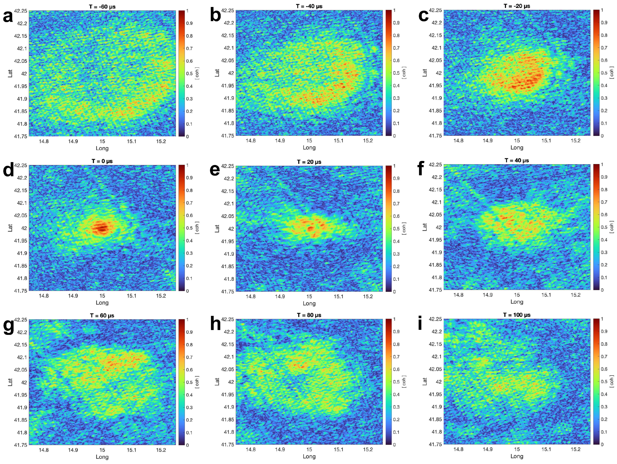
For the simulated lightning location L, the filtered waveforms should be well-defined impulses at the lightning occurrence time. The coherency waveform of these output impulse waveforms is shown in Figure 6b. It can be seen that the coherency waveform of the filtered recorded waveforms only has one sharp peak. The coherency reaches the maximum of 0.76 at 5 s. This time coincides with the local maximum time in the coherency waveform of recorded waveforms (upper figure in Figure 6a) in Section 5.1. Figure 16a–h are the coherency maps for the time frame −60 to 100 s. The maximum coherency shows in the time frame t = 0 s, while no skywave is shown in these coherency maps. In this work, the filtered recorded waveform only has a sharp impulse to represent the lightning event. Therefore, even if the impulse still has a width, which results in the apparent movement of the lightning location, the maximum value only exists at the simulated lightning location at the lightning occurrence time.
The amplitude of the filtered waveforms is also used for the interferometric method for comparison. The averaged amplitude waveform of these output impulse waveforms is shown in Figure 8b. It can be seen that this waveform has a sharp peak at the lightning occurrence time t = 0 s; however, the peak is ∼0.06. This peak value is also illustrated in the amplitude maps in Figure 17. The interferometric method using the amplitude of filtered waveforms also shows a single maximum area associated with the ground wave in amplitude maps.
In this method, the input waveforms are scaled amplitude waveforms—that is, the amplitude waveforms are scaled to their ground wave maximum. The amplitude waveforms from the amplitude waveform bank which are used to calculate the impulse response functions are also scaled to their ground wave maximum. However, the input waveforms contain much more high-frequency components than the amplitude waveforms from the amplitude waveform bank. Even though both of them are scaled to the ground wave maximum, they contain different ratios of different frequency components. Therefore, the output waveforms , before applying the 50 kHz low-pass filter, should contain more high-frequency components. After that low-pass filter, the output signal loses a large amount of energy and has an impulse peak much smaller than 1. The problem with this method is that the lost energy cannot be quantified and depends on individual cases. Therefore, it is difficult to find a constant threshold for lightning detection purposes.
8. Discussion
In this work, coherency maps are created based on the lightning waveforms that are referenced at their occurrence time. Therefore, for each test pixel, the coherency needs to be calculated based on the relative distance between the test pixel P to n-th receiver location and the lightning location L to n-th receiver. To determine a single location for the lightning event without interference from skywaves, two methods can be used. The first method is to pre-locate the lightning event into a large area. Then, only the waveforms recorded by nearby receivers to locate the lightning are used. The waveforms recorded by the adjacent receivers have a larger ground wave value compared to skywaves. In addition, the time delay between the ground wave and skywaves is also large, which is suitable for identifying the ground wave. If the receivers of the network distribute evenly around the lightning event, there are no apparent lightning movements, and the location with maximum coherency associated with the ground wave is the simulated lightning location. The second method is more straightforward. In this method, there is no need to select the receiver network because the distances are selected by the pixel and the receiver locations. For recorded waveform, the impulse response function filter is applied so that the lightning event is represented by the Kronecker delta impulse. The calculated dynamic coherency maps still exhibit lightning movements because of the impulse width. However, the coherency only reaches the maximum at the lightning location at the occurrence time.
These two solutions are also applied to amplitude maps. For the small network solution, the interferometric method with amplitude has a critical requirement for baseline. It is reported by Zhu et al. [21] that the amplitude can effectively work in LF with the interferometric method. However, in their study, the baselines are between 30–60 km, which means the recorded ground wave is sharp with few attenuation effects, and no skywave exists near the ground wave time range. In our case, even with a network of 10 receivers, the propagation distances are between 140 km and 370 km, which leads to an average time delay between the ground wave and the first skywave of 160 s. This time delay is equivalent to ∼50 km distance delay, which is ∼0.5 degree on the map. It explains the existence of the first skywave in Figure 14.
As for the interferometric method using amplitude with filtered waveforms, the results clearly show the lightning appearance. However, unlike coherency, which has a standard value range, i.e., 0–1, which only depends on the case number N, the output amplitude value largely depends on the signal to noise ratio of the individual input waveform. In practice, it is hard to set a threshold value for lightning detection purposes.
In real-life lightning location work, the coherency map can be calculated in real-time using UTC time. For the test pixel P at the time , the corresponding point recorded at the n-th receiver is , where is the propagation time between the test pixel P and the n-th receiver by assuming the propagation velocity equals to the speed of light. The coherency is
If the second method is used, instead of using a single time stamp , a waveform is needed to apply the filter. Based on different coherency map sizes, the different lengths of waveforms, which take the point as the reference, can be extracted. The impulse response function filter for the test pixel P is the waveform from the amplitude waveform bank with the distance of , which is the propagation distance between the test pixel P and the n-th receiver.
The limitation of the interferometric method is that the performance is dependent on the number of receivers used to work synchronously and ∼10 receivers are needed to give a reliable coherency map while the traditional TOA technique requires a minimum of 4 receivers.
There are also limitations to the data used. In this work, all the data used for the simulation works are collected from Bath and Rustrel on the same days. As these events are all generated from the same storms and recorded at the same locations, they have similar geographic environments, atmospheric conditions, and propagation paths. In the future, more data would be evaluated to explore the sensitivity of the simulated results with respect to different conditions.
9. Summary
This contribution introduces a simulation work that uses the interferometric method to locate lightning events in a long-range system. In this section, we provide a more detailed plan for future work of constructing a real-time long-range interferometric system and detecting the location of lightning by calculating the coherency map.
There are 8 steps to achieve this aim: (1). Segment the area of interest into pixels. The area of interest is usually the area inside of the receiver network which has a better detection accuracy. (2). For a given time T and a given pixel P, calculate the distances between P and the n-th receiver. (3). Use the distances to extract a set of averaged waveforms from the amplitude waveform bank. Calculate the inverse impulse response function of these waveforms as a set of inverse filters. (4). Take the recorded electric field waveforms of receivers. In this step, the lightning propagation time is considered and the time of at n-th receiver is referenced to . Each waveform has a duration that covers -0.5 ms before and 2 ms after the time 0. (5). Calculate the filtered waveforms by applying the inverse filters to the recorded waveform set. (6). Calculate the coherency waveform of the filtered waveforms. The coherency of time 0 is the coherency of the given time T at the given location P. (7). Repeat the process for all the pixels of the area of interest to form a coherency map at the given time T. (8). The coherency threshold is determined by the receiver number. The area in the map that has a coherency value larger than the threshold coherency would be considered a significant event. The pixel with the largest coherency inside the area is considered to be the lightning location.
While the TOA technique tries to locate the lightning in a best-fit location, this method scans through the whole area of interest and detects lightning events by finding the areas with coherency larger than the threshold coherency. The computation time would be large as this method needs to calculate the coherency for all the pixels. In contrast, this method is less affected by the skywave interference in a long-range system.
10. Conclusions
This contribution has investigated a novel complex interferometric method for lightning detection and location. The sensitivity maps using TOA and coherency are produced to study the location accuracy caused by the uncertainty introduced by the physical processes involved, i.e., the varying properties of individual lightning events and the subsequent wave propagation. The coherency is quantitatively studied for both lightning events and noises based on different event numbers and receiver locations. These values are used as the reference for the later coherency map. The waveforms from the amplitude waveform bank are first used to study the complex interferometric method. Then, the waveforms of individual events are used to study the dynamic map using both amplitude and coherency. It is shown that the coherency works better at long-range mapping in this work with less interfering first skywave, a better arrival time of ground wave, and a higher signal to noise ratio for the ground wave. A small network is simulated for the complex interferometric method, whose performance has met the expectation for coherency, while the amplitude method has critical requirements for the network baseline. The filtered waveforms are also used to map the lightning event without interference from skywaves. The coherency maps using the filtered waveforms can clearly show a single maximum area for each lightning event, while the coherency only depends on the case number. The amplitude largely depends on the signal to noise ratio of the individual input waveform. The interferometric method helps to better identify the lightning ground wave and reduce the interference from the skywaves. To reduce the lightning apparent movement, which is a by-product of the interferometric method in the long-range network, two methods are presented here. In the future, it is planned to expand the simulation work with data reflecting a variety of ionospheric and geographic scenarios.
Author Contributions
X.B. conducted the analysis and wrote the paper, and M.F. assisted with conceiving the concept of the paper. All authors have read and agreed to the published version of the manuscript.
Funding
The work of X.B. was sponsored by URSA under the project grant number EA-EE1250. The work of M.F. was sponsored by the Royal Society (UK) grant NMG/R1/180252 and the Natural Environment Research Council (UK) under grants NE/L012669/1 and NE/H024921/1.
Data Availability Statement
The data used for this publication will be available from https://doi.org/10.15125/BATH-01211.
Acknowledgments
The authors wish to thank Stephane Pedeboy at Méteorage for access to selected lightning flash data, the team of the Laboratory Souterrain a Bas Bruit (LSBB) in Rustrel for their generous hospitality, Adam Peverell for extracting and communicating the data, Yuqing Liu, Mert Yücemöz, Serge Soula, Jean-Louis Pinçon, Franck Elie, and Matthieu Garnung for assisting with the acquisition of the electric field data used in this study, and the reviewers for their assistance to improve the quality of the manuscript.
Conflicts of Interest
The authors declare no conflict of interest. The funders had no role in the design of the study; in the collection, analyses, or interpretation of data; in the writing of the manuscript; or in the decision to publish the results.
Abbreviations
The following abbreviations are used in this manuscript:
| CG | cloud-to-ground |
| ENTLN | Earth Networks Total Lightning Network |
| IC | in-cloud discharge |
| LF | low frequency |
| LLS | Lightning location system |
| LSBB | Laboratory Souterrain a Bas Bruit |
| NLDN | National Lightning Detection Network |
| TOA | time of arrival |
| VHF | very high frequency |
| VLF | very low frequency |
| WGS84 | World Geodetic System |
Appendix A. Table of Symbols
: amplitude value of the simulated lightning location L
: the amplitude waveform recorded at n-th receiver
c: the speed of light
: coherency
: peak coherency associated with the ground wave
: threshold coherency
: the distance difference between the test pixel toward n-th and -th receivers
: the distance between the test pixel and the n-th receiver
: the distance between the simulated lightning location L and n-th receiver.
: the distance between the test pixel P and n-th receiver
: the distance difference between the determined lightning location, which considering the time uncertainty, and the test pixel
: the distance difference between the test pixel P to n-th receiver location and the lightning location L to n-th receiver
L: the simulated lightning location
N: receiver number, i.e., case number
: random time delay
P: test pixel location
q: quality
R the standout level of the ground wave
: the ratio between the calculated peak current and the peak current reported by Méteorage
: the propagation time differences between the test pixel toward n-th and -th receivers
: the propagation time differences between the test pixel toward n-th and -th receivers with time uncertainty
the time point used from the n-th waveform
: the target time of the map
: the impulse response functions at distance d
: the impulse response function at the distance
: the time delay of the test pixel P compared to the simulated lightning location L for n-th receiver
: the analytic signal recorded at the n-th receiver
: impulse response function filtered waveform at n-th receiver
References
- Rakov, V.A.; Uman, M.A. Lightning: Physics and Effects; Cambridge University Press: New York, NY, USA, 2003. [Google Scholar] [CrossRef]
- Taylor, W.L. Daytime attenuation rates in the very low frequency band using atmospherics. J. Res. Natl. Inst. Stand. Technol. 1960, 64D, 349. [Google Scholar] [CrossRef]
- Cummins, K.L.; Murphy, M.J. An Overview of Lightning Locating Systems: History, Techniques, and Data Uses, With an In-Depth Look at the U.S. NLDN. IEEE Trans. Electromagn. Compat. 2009, 51, 499–518. [Google Scholar] [CrossRef]
- Cummins, K.L.; Krider, E.; Malone, M. The US National Lightning Detection Network/sup TM/ and applications of cloud-to-ground lightning data by electric power utilities. IEEE Trans. Electromagn. Compat. 1998, 40, 465–480. [Google Scholar] [CrossRef] [Green Version]
- Nag, A.; Murphy, M.J.; Schulz, W.; Cummins, K.L. Lightning locating systems: Insights on characteristics and validation techniques. Earth Space Sci. 2015, 2, 65–93. [Google Scholar] [CrossRef]
- Jones, D.L. ELF Sferics and Lightning Effects on the Middle and upper Atmosphere. In Modern Radio Science 1999; Stuchley, M.A., Ed.; Oxford University Press: Oxford, UK, 1999; pp. 171–189. [Google Scholar] [CrossRef]
- Cummins, K.L.; Murphy, M.J.; Bardo, E.A.; Hiscox, W.L.; Pyle, R.B.; Pifer, A.E. A Combined TOA/MDF Technology Upgrade of the U.S. National Lightning Detection Network. J. Geophys. Res. Atmos. 1998, 103, 9035–9044. [Google Scholar] [CrossRef]
- Marchand, M.; Hilburn, K.; Miller, S.D. Geostationary Lightning Mapper and Earth Networks Lightning Detection Over the Contiguous United States and Dependence on Flash Characteristics. J. Geophys. Res. Atmos. 2019, 124, 11552–11567. [Google Scholar] [CrossRef]
- Said, R.K.; Murphy, M. GLD360 upgrade: Performance analysis and applications. In Proceedings of the 24th International Lightning Detection Conference and 6th International Lightning Meteorology Conference, San Diego, CA, USA, 18–21 April 2016. [Google Scholar]
- Abarca, S.F.; Corbosiero, K.L.; Galarneau, T.J. An evaluation of the Worldwide Lightning Location Network (WWLLN) using the National Lightning Detection Network (NLDN) as ground truth. J. Geophys. Res. 2010, 115, D18206. [Google Scholar] [CrossRef]
- Pédeboy, S. Analysis of the French lightning locating system location accuracy. In Proceedings of the 2015 International Symposium on Lightning Protection (XIII SIPDA), Balneario Camboriu, Brazil, 28 September–2 October 2015; pp. 337–341. [Google Scholar] [CrossRef]
- Mazur, V.; Williams, E.; Boldi, R.; Maier, L.; Proctor, D.E. Initial comparison of lightning mapping with operational time-of-arrival and interferometric systems. J. Geophys. Res. Atmos. 1997, 102, 11071–11085. [Google Scholar] [CrossRef]
- Rakov, V.A. Electromagnetic Methods of Lightning Detection. Surv. Geophys. 2013, 34, 731–753. [Google Scholar] [CrossRef]
- Proctor, D.E. VHF radio pictures of cloud flashes. J. Geophys. Res. Oceans 1981, 86, 4041–4071. [Google Scholar] [CrossRef]
- Shao, X.M.; Holden, D.N.; Rhodes, C.T. Broad band radio interferometry for lightning observations. Geophys. Res. Lett. 1996, 23, 1917–1920. [Google Scholar] [CrossRef]
- Sun, Z.; Qie, X.; Liu, M.; Cao, D.; Wang, D. Lightning VHF radiation location system based on short-baseline TDOA technique—Validation in rocket-triggered lightning. Atmos. Res. 2013, 129–130, 58–66. [Google Scholar] [CrossRef]
- Stock, M.; Akita, M.; Krehbiel, P.R.; Rison, W.; Edens, H.E.; Kawasaki, Z.; Stanley, M.A. Continuous broadband digital interferometry of lightning using a generalized cross-correlation algorithm. J. Geophys. Res. Atmos. 2014, 119, 3134–3165. [Google Scholar] [CrossRef]
- Stock, M.; Krehbiel, P. Multiple baseline lightning interferometry - Improving the detection of low amplitude VHF sources. In Proceedings of the 2014 International Conference on Lightning Protection (ICLP), Beijing, China, 11–18 October 2014; pp. 293–300. [Google Scholar] [CrossRef]
- Lyu, F.; Cummer, S.A.; Solanki, R.; Weinert, J.; Mctague, L.; Katko, A.; Barrett, J.; Zigoneanu, L.; Xie, Y.; Wang, W. A low-frequency near-field interferometric-TOA 3-D Lightning Mapping Array. Geophys. Res. Lett. 2014, 41, 7777–7784. [Google Scholar] [CrossRef]
- Zhu, Y.; Bitzer, P.; Stewart, M.; Podgorny, S.; Corredor, D.; Burchfield, J.; Carey, L.; Medina, B.; Stock, M. Huntsville Alabama Marx Meter Array 2: Upgrade and Capability. Earth Space Sci. 2020, 7, e2020EA001111. [Google Scholar] [CrossRef] [Green Version]
- Zhu, Y.; Stock, M.; Bitzer, P. A new approach to map lightning channels based on low-frequency interferometry. Atmos. Res. 2021, 247, 105139. [Google Scholar] [CrossRef]
- Inan, U.S.; Cummer, S.A.; Marshall, R.A. A survey of ELF and VLF research on lightning-ionosphere interactions and causative discharges. J. Geophys. Res. Space Phys. 2010, 115, A00E36. [Google Scholar] [CrossRef] [Green Version]
- Silber, I.; Price, C.; Galanti, E.; Shuval, A. Anomalously strong vertical magnetic fields from distant ELF/VLF sources. J. Geophys. Res. Space Phys. 2015, 120, 6036–6044. [Google Scholar] [CrossRef]
- Schonland, B.F.J.; Elder, J.S.; Hodges, D.B.; Phillips, W.E.; Van Wyk, J.W. The wave form of atmospherics at night. Proc. R. Soc. A Math. Phys. Eng. Sci. 1940, 176, 180–202. [Google Scholar] [CrossRef] [Green Version]
- Leal, A.F.R.; Rakov, V.A. Characterization of Lightning Electric Field Waveforms Using a Large Database: 1. Methodology. IEEE Trans. Electromagn. Compat. 2021, 63, 1155–1162. [Google Scholar] [CrossRef]
- Chapman, J.; Pierce, E. Relations between the Character of Atmospherics and Their Place of Origin. Proc. IRE 1957, 45, 804–806. [Google Scholar] [CrossRef]
- Cummer, S.A.; Inan, U.S.; Bell, T.F. Ionospheric D region remote sensing using VLF radio atmospherics. Radio Sci. 1998, 33, 1781–1792. [Google Scholar] [CrossRef] [Green Version]
- Zhou, X.; Wang, J.; Ma, Q.; Huang, Q.; Xiao, F. A method for determining D region ionosphere reflection height from lightning skywaves. J. Atmos. Sol.-Terr. Phys. 2021, 221, 105692. [Google Scholar] [CrossRef]
- Burkholder, B.S.; Hutchins, M.L.; McCarthy, M.P.; Pfaff, R.F.; Holzworth, R.H. Attenuation of lightning-produced sferics in the Earth-ionosphere waveguide and low-latitude ionosphere. J. Geophys. Res. Space Phys. 2013, 118, 3692–3699. [Google Scholar] [CrossRef]
- Caligaris, C.; Delfino, F.; Procopio, R. Cooray–Rubinstein Formula for the Evaluation of Lightning Radial Electric Fields: Derivation and Implementation in the Time Domain. IEEE Trans. Electromagn. Compat. 2008, 50, 194–197. [Google Scholar] [CrossRef]
- Cooray, V. Propagation Effects Due to Finitely Conducting Ground on Lightning-Generated Magnetic Fields Evaluated Using Sommerfeld’s Integrals. IEEE Trans. Electromagn. Compat. 2009, 51, 526–531. [Google Scholar] [CrossRef]
- Hou, W.; Zhang, Q.; Zhang, J.; Wang, L.; Shen, Y. A New Approximate Method for Lightning-Radiated ELF/VLF Ground Wave Propagation over Intermediate Ranges. Int. J. Antennas Propag. 2018, 2018, 1–10. [Google Scholar] [CrossRef] [Green Version]
- Shao, X.M.; Jacobson, A.R. Model Simulation of Very Low-Frequency and Low-Frequency Lightning Signal Propagation Over Intermediate Ranges. IEEE Trans. Electromagn. Compat. 2009, 51, 519–525. [Google Scholar] [CrossRef]
- Pessi, A.T.; Businger, S.; Cummins, K.L.; Demetriades, N.W.S.; Murphy, M.; Pifer, B. Development of a Long-Range Lightning Detection Network for the Pacific: Construction, Calibration, and Performance*. J. Atmos. Ocean. Technol. 2009, 26, 145–166. [Google Scholar] [CrossRef] [Green Version]
- Mezentsev, A.; Füllekrug, M. Mapping the radio sky with an interferometric network of low-frequency radio receivers. J. Geophys. Res. Atmos. 2013, 118, 8390–8398. [Google Scholar] [CrossRef] [Green Version]
- Said, R.K.; Inan, U.S.; Cummins, K.L. Long-range lightning geolocation using a VLF radio atmospheric waveform bank. J. Geophys. Res. Atmo. 2010, 115, D23108. [Google Scholar] [CrossRef] [Green Version]
- Li, J.; Dai, B.; Zhou, J.; Zhang, J.; Zhang, Q.; Yang, J.; Wang, Y.; Gu, J.; Hou, W.; Zou, B.; et al. Preliminary Application of Long-Range Lightning Location Network with Equivalent Propagation Velocity in China. Remote Sens. 2022, 14, 560. [Google Scholar] [CrossRef]
- Taner, M.T.; Koehler, F.; Sheriff, R.E. Complex seismic trace analysis. Geophysics 1979, 44, 1041–1063. [Google Scholar] [CrossRef]
- Liu, Z.; Koh, K.L.; Mezentsev, A.; Enno, S.E.; Sugier, J.; Füllekrug, M. Variable phase propagation velocity for long-range lightning location system. Radio Sci. 2016, 51, 1806–1815. [Google Scholar] [CrossRef] [Green Version]
- Liu, Z.; Koh, K.L.; Mezentsev, A.; Enno, S.E.; Sugier, J.; Fullekrug, M. Lightning sferics: Analysis of the instantaneous phase and frequency inferred from complex waveforms. Radio Sci. 2018, 53, 448–457. [Google Scholar] [CrossRef]
- Füllekrug, M.; Liu, Z.; Koh, K.; Mezentsev, A.; Pedeboy, S.; Soula, S.; Enno, S.E.; Sugier, J.; Rycroft, M.J. Mapping lightning in the sky with a mini array. Geophys. Res. Lett. 2016, 43, 10448–10454. [Google Scholar] [CrossRef] [Green Version]
- Bai, X.; Füllekrug, M. Coherency of Lightning Sferics. Radio Sci. 2022, 57, e2021RS007347. [Google Scholar] [CrossRef]
- Füllekrug, M. Wideband digital low-frequency radio receiver. Meas. Sci. Technol. 2010, 21, 015901. [Google Scholar] [CrossRef]
- Liu, Z. Investigation of Low Frequency Electromagnetic Waves for Long-Range Lightning Location. Ph.D. Thesis, University of Bath, Bath, UK, 2017. [Google Scholar]
- Füllekrug, M.; Koh, K.; Liu, Z.; Mezentsev, A. Detection of Low-Frequency Continuum Radiation. Radio Sci. 2018, 53, 1039–1050. [Google Scholar] [CrossRef] [Green Version]
- Kolmašová, I.; Santolík, O.; Farges, T.; Cummer, S.A.; Lán, R.; Uhlíř, L. Subionospheric propagation and peak currents of preliminary breakdown pulses before negative cloud-to-ground lightning discharges. Geophys. Res. Lett. 2016, 43, 1382–1391. [Google Scholar] [CrossRef]
- Kašpar, P.; Santolík, O.; Kolmašová, I.; Farges, T. A model of preliminary breakdown pulse peak currents and their relation to the observed electric field pulses. Geophys. Res. Lett. 2017, 44, 596–603. [Google Scholar] [CrossRef]
Figure 1.
(a) Interpolated waveform bank spectrum (190–2150 km). (b) Sensitivity map using quality q value. The receivers are marked in red dots. The range is 35°N to 60°N for latitude and 10°W to 25°E for longitude with a pixel resolution of 0.5° × 0.5°.
Figure 1.
(a) Interpolated waveform bank spectrum (190–2150 km). (b) Sensitivity map using quality q value. The receivers are marked in red dots. The range is 35°N to 60°N for latitude and 10°W to 25°E for longitude with a pixel resolution of 0.5° × 0.5°.

Figure 2.
(a) An example of coherency waveforms calculated over randomly selected individual events with the case numbers 10, 40, 70, and 100. (b) The peak coherency (black), threshold coherency (blue), and ratio R (red) with different event numbers. (c) coherency based on different receiver pairs. The peak coherency are the lines larger than 0.4 while the threshold coherency are the lines lower than 0.4. The threshold value of 0.4 is marked with a red dashed line. (d) Ratio R values with different selections of receiver locations. In both (c,d), the upper figure shows the coherency at Bath (red), Toulouse (green), Orleans (black), and Rustrel (blue). The middle figure shows the coherency for the location pairs Bath–Toulouse (red), Bath–Orleans (green), Bath–Rustrel (black), Toulouse–Orleans (blue), Toulouse–Rustrel (sky blue), and Orleans–Rustrel (purple). The bottom figure shows the coherency for the location sets Toulouse–Orleans–Rustrel (red), Bath–Orleans–Rustrel (green), Bath–Toulouse–Rustrel (black), and Bath–Toulouse–Orleans (blue).

Figure 3.
(a) Distance distribution for events recorded from different locations. (b) Noise coherency with different event numbers. This figure shows theoretical coherency noise values (blue), the coherency of noises recorded at Bath (yellow), Toulouse (purple), Orleans (green), and Rustrel (sky, blue), and event threshold coherency (red).

Figure 4.
(a) Simulated lightning locations (red open circle and red dot) and receiver distribution in Europe (all the dots except two red dots). The red open circle is the simulated lightning location using the averaged waveforms from the amplitude waveform bank, and the red dot is the simulated lightning location of 15°E and 42°S. Yellow dots are the receiver used in the simulation with averaged waveforms from the amplitude waveform bank; black dots are the 10 receivers used in a small receiver network (N = 10); the black dots and green dots are the 20 receivers used in small receiver network (N = 20). (b) The calculated coherency map by using the amplitude waveforms from the amplitude waveform bank. The coherency map has a latitude and longitude range of 0.5° × 0.5°, with a precision of 0.001° × 0.001°.

Figure 5.
Amplitude waveforms from the amplitude waveform bank used to simulate the coherency map.

Figure 6.
(a) Coherency waveforms used in the simulation with 105 receiver network. Calculated coherency waveform of the selected individual events (upper) and the coherency waveform of 1150 km from the coherency waveform bank (bottom). The ground wave maxima are marked with red dots, and the skywave maxima are marked with red open circles. (b) The coherency waveform calculated by the filtered waveforms. The maximum is marked with a red dot.

Figure 7.
The coherency maps with 105 receiver network with a simulated lightning location of 15°E and 42°S. Each sub-figure (a–l) is the coherency map at a different time.
Figure 7.
The coherency maps with 105 receiver network with a simulated lightning location of 15°E and 42°S. Each sub-figure (a–l) is the coherency map at a different time.

Figure 8.
(a) Amplitude waveforms used in the simulation with 105 receiver network. The middle figure is the scaled amplitude waveform; the bottom figure is the ratioed amplitude waveform; and the upper figure is the amplitude waveform of 1150 km from the amplitude waveform bank. The ground wave maxima are marked with red dots, and the skywave maxima are marked with red open circles. (b) The amplitude waveform calculated by the filtered waveforms. The maximum is marked with a red dot.

Figure 9.
The scaled amplitude maps with 105 receiver network with a simulated lightning location of 15°E and 42°S. Each sub-figure (a–l) is the amplitude map of a different time frame.
Figure 9.
The scaled amplitude maps with 105 receiver network with a simulated lightning location of 15°E and 42°S. Each sub-figure (a–l) is the amplitude map of a different time frame.

Figure 10.
(a) Coherency waveforms used in the simulation with a small network (N = 10). (b) Coherency waveforms used in the simulation with a small network (N = 20). For both Figures (a,b), the upper figure is the calculated coherency waveform and the bottom figure is the coherency waveform of 270 km and 410 km, respectively, from the coherency waveform bank. In all the figures, the ground wave maxima are marked with red dots.

Figure 11.
The coherency maps with a small receiver network with a simulated lightning location of 15°E and 42°S (N = 10). Each sub-figure (a–i) is the coherency map at a different time.
Figure 11.
The coherency maps with a small receiver network with a simulated lightning location of 15°E and 42°S (N = 10). Each sub-figure (a–i) is the coherency map at a different time.

Figure 12.
The coherency maps with a small receiver network with a simulated lightning location of 15°E and 42°S (N = 20). Each sub-figure (a–i) is the coherency map at a different time.
Figure 12.
The coherency maps with a small receiver network with a simulated lightning location of 15°E and 42°S (N = 20). Each sub-figure (a–i) is the coherency map at a different time.

Figure 13.
(a) Amplitude waveforms used in the simulation with a small network (N = 10). (b) Amplitude waveforms used in the simulation with a small network (N = 20). For both figures (a,b), the upper figures are the averaged waveforms from the amplitude waveform bank (270 km and 410 km); the middle figures are the scaled amplitude waveforms; and the bottom figures are the ratioed amplitude waveforms. In all the figures, the ground wave maxima are marked with red dots.

Figure 14.
The scaled amplitude maps with a small receiver network with a simulated lightning location of 15°E and 42°S (N = 10).
Figure 14.
The scaled amplitude maps with a small receiver network with a simulated lightning location of 15°E and 42°S (N = 10).

Figure 15.
The scaled amplitude maps with a small receiver network with a simulated lightning location of 15°E and 42°S (N = 20).
Figure 15.
The scaled amplitude maps with a small receiver network with a simulated lightning location of 15°E and 42°S (N = 20).

Figure 16.
The coherency maps using the impulse response function filtered waveforms with a simulated lightning location of 15°E and 42°S. Each sub-figure (a–i) is the coherency map at a different time.
Figure 16.
The coherency maps using the impulse response function filtered waveforms with a simulated lightning location of 15°E and 42°S. Each sub-figure (a–i) is the coherency map at a different time.

Figure 17.
The amplitude maps using the impulse response function filtered waveforms with a simulated lightning location of 15°E and 42°S. Each sub-figure (a–i) is the amplitude map at a different time.
Figure 17.
The amplitude maps using the impulse response function filtered waveforms with a simulated lightning location of 15°E and 42°S. Each sub-figure (a–i) is the amplitude map at a different time.

Disclaimer/Publisher’s Note: The statements, opinions and data contained in all publications are solely those of the individual author(s) and contributor(s) and not of MDPI and/or the editor(s). MDPI and/or the editor(s) disclaim responsibility for any injury to people or property resulting from any ideas, methods, instructions or products referred to in the content. |
© 2023 by the authors. Licensee MDPI, Basel, Switzerland. This article is an open access article distributed under the terms and conditions of the Creative Commons Attribution (CC BY) license (https://creativecommons.org/licenses/by/4.0/).
Share and Cite
MDPI and ACS Style
Bai, X.; Füllekrug, M. Long-Range Lightning Interferometry Using Coherency. Remote Sens. 2023, 15, 1950. https://doi.org/10.3390/rs15071950
AMA Style
Bai X, Füllekrug M. Long-Range Lightning Interferometry Using Coherency. Remote Sensing. 2023; 15(7):1950. https://doi.org/10.3390/rs15071950
Chicago/Turabian StyleBai, Xue, and Martin Füllekrug. 2023. "Long-Range Lightning Interferometry Using Coherency" Remote Sensing 15, no. 7: 1950. https://doi.org/10.3390/rs15071950
Note that from the first issue of 2016, this journal uses article numbers instead of page numbers. See further details here.