


Riparian Plant Evapotranspiration and Consumptive Use for Selected Areas of the Little Colorado River Watershed on the Navajo Nation
 , ,
, ,
Abstract
:1. Introduction
1.1. Terms
1.2. General Methods as Applied to Terms
1.3. Objectives
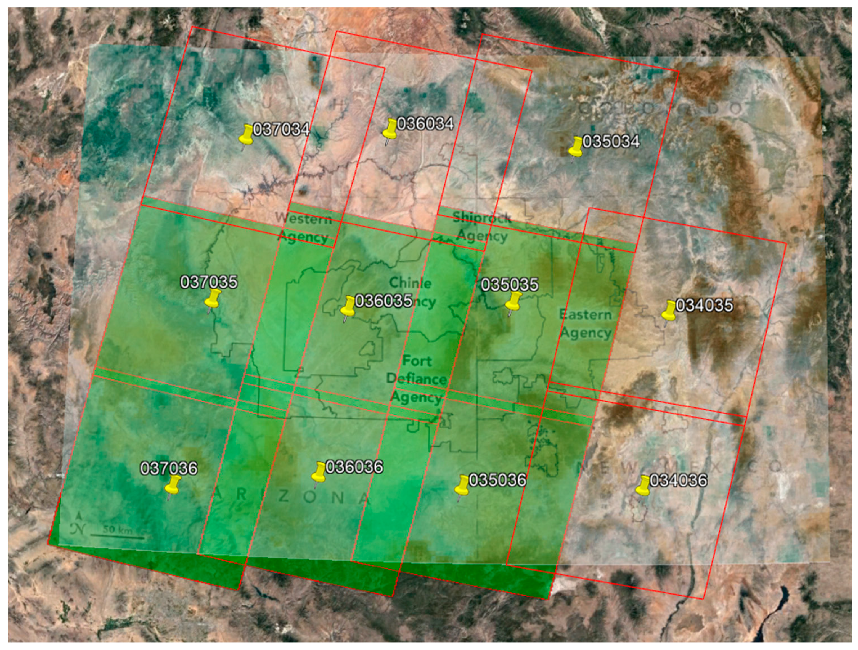
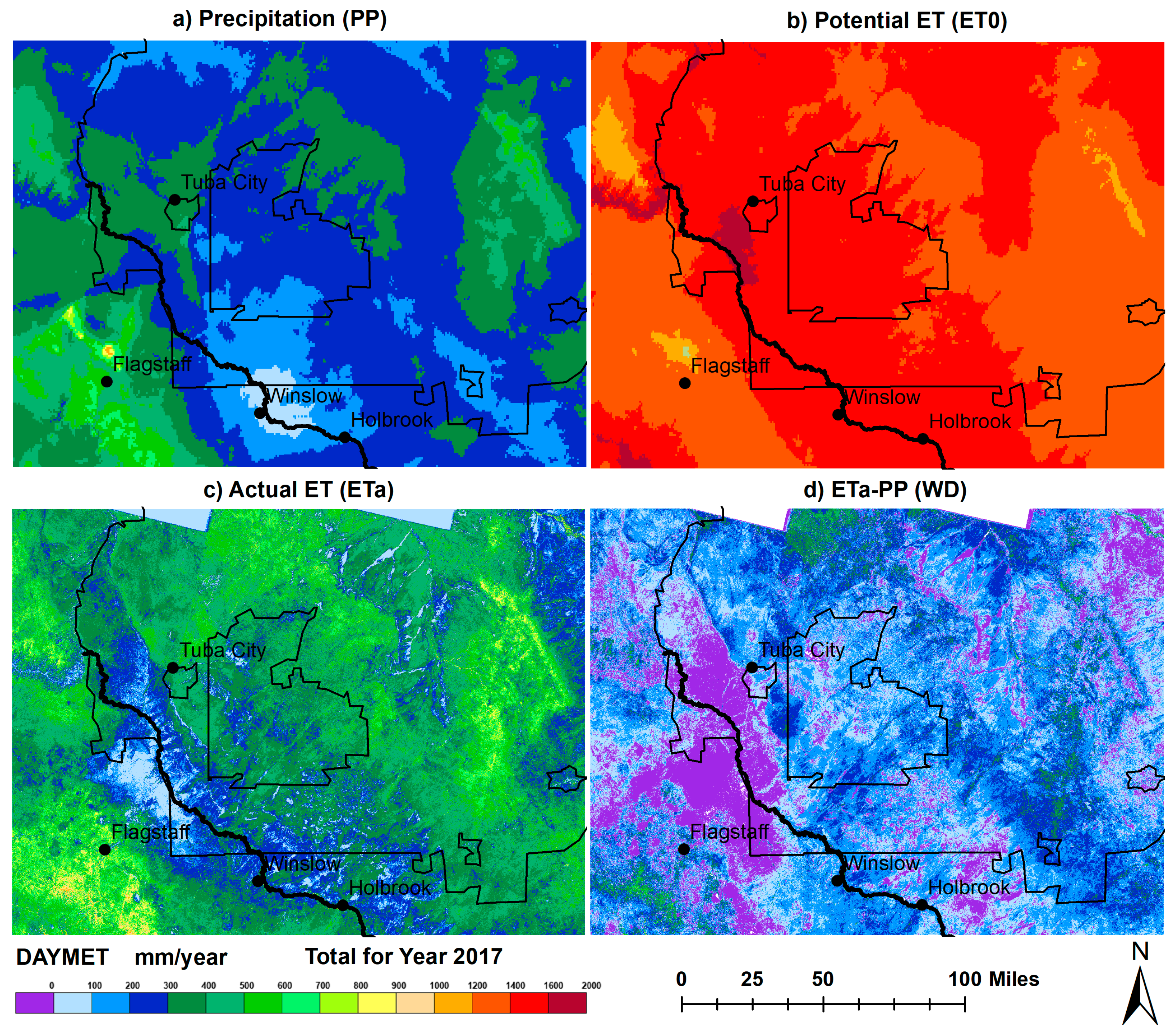
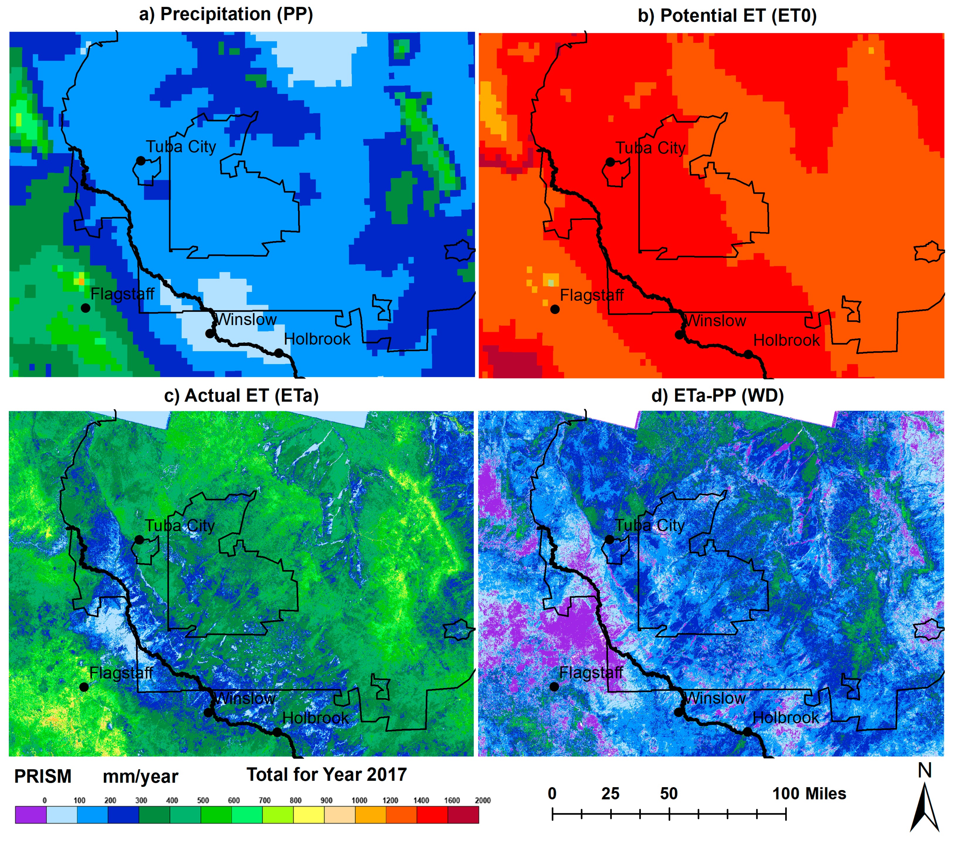
- Acquire daily weather data from two gridded sources, Daymet (1 km) and PRISM (4 km) and Landsat 8/OLI (30-m) scenes that cover the northeastern corner of Arizona.
- Calculate the daily ETo using the input weather data.
- Standardize all computations to a 16-day time-step that matches the Landsat overpass dates to reduce outliers, then produce PP, ETo, ETa and WD.
- Develop annual maps of PP, ETo, Eta, and WD water metrics at the Landsat 30 m spatial resolution.
- Estimate riparian plant water use by three different and spatially explicit methods:
- a polygon-based ‘hand-digitization’ method of the riparian vegetative cover, and
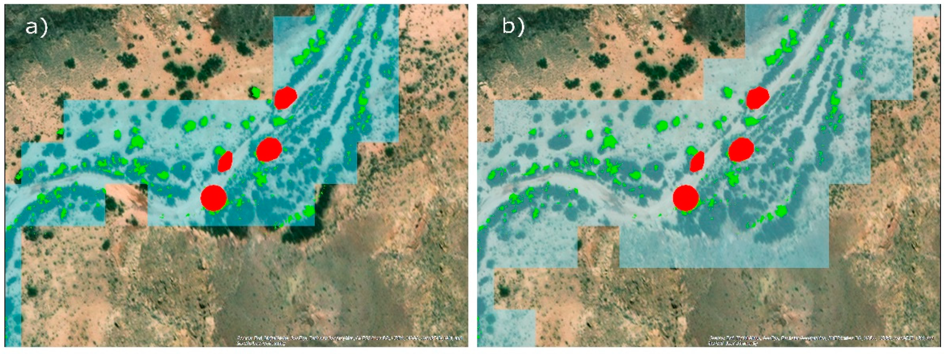
- a newly devised automatic rasterization method that counts any Landsat 30 m pixels containing vegetation as riparian using two levels of detail: a ‘conservative’ and ‘best-approximation’ to estimate the riparian area. The ‘conservative’ method considers only pixels with >50% of vegetation cover, the ‘best-approximation’ method considers any pixels with vegetation which results in a larger area estimate. We then calculate CU using any of the above methods for estimating riparian area.
2. Data and Methods
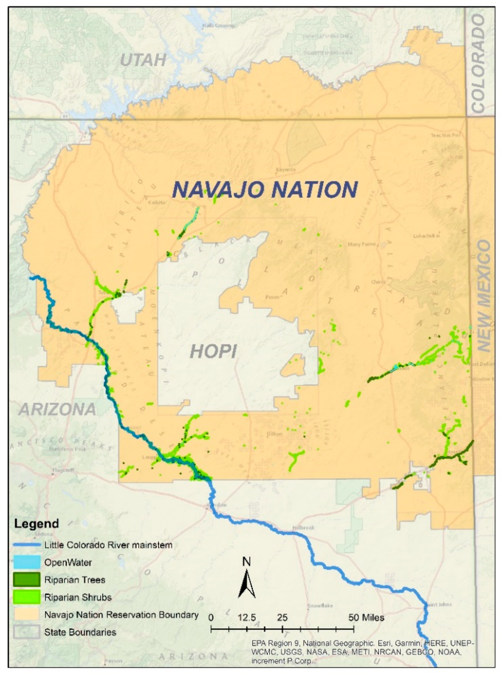
2.1. Study Area
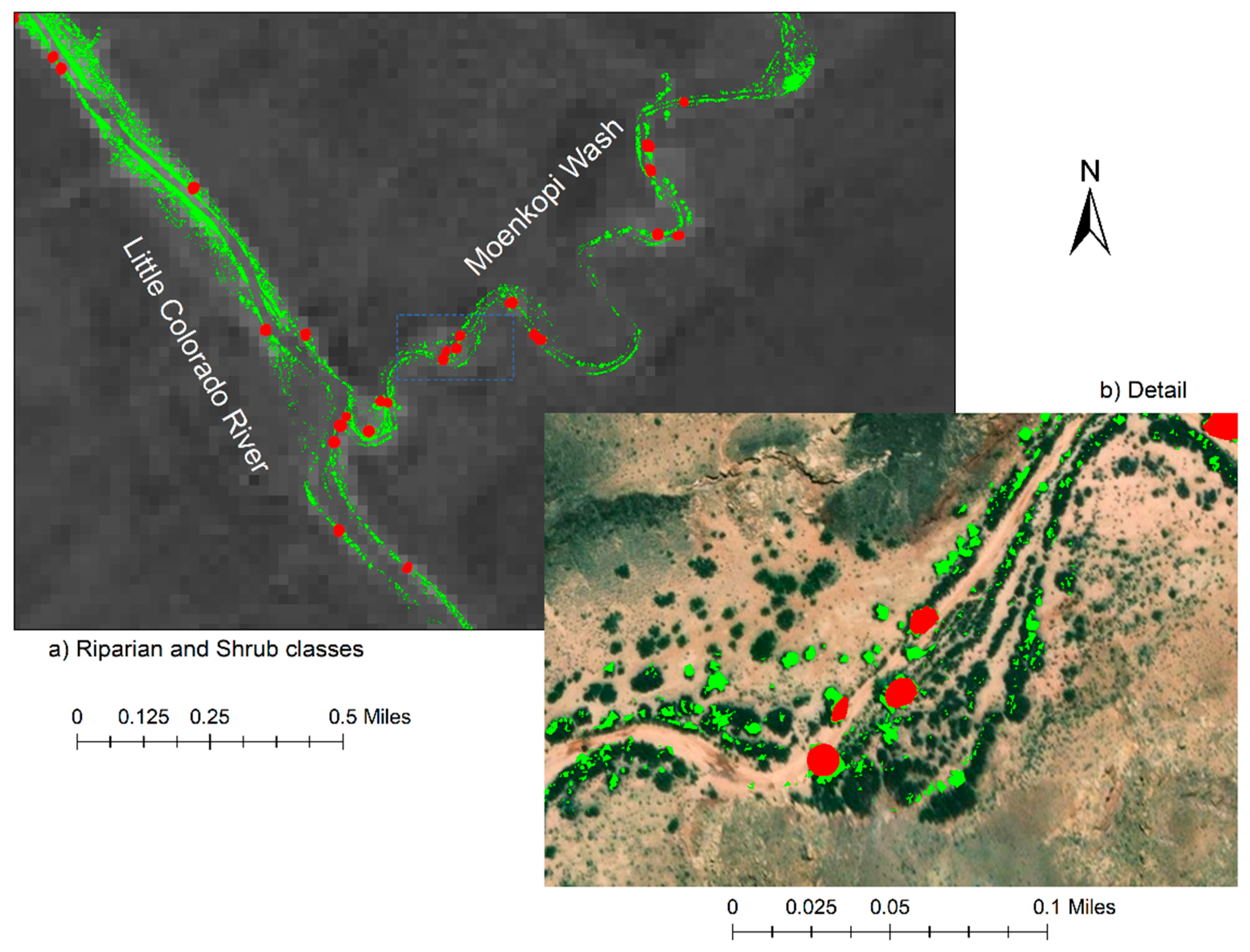
2.2. Area Delineation of Riparian Trees and Shrubs
2.2.1. Vector-Based Riparian Area Delineation
2.2.2. Raster-Based Riparian Area Delineation
2.3. Acquired Landsat-8/OLI Satellite Imagery
2.4. Weather Data Acquisition on the Navajo Reservation
2.5. Vegetation Index-Based Evapotranspiration Estimation
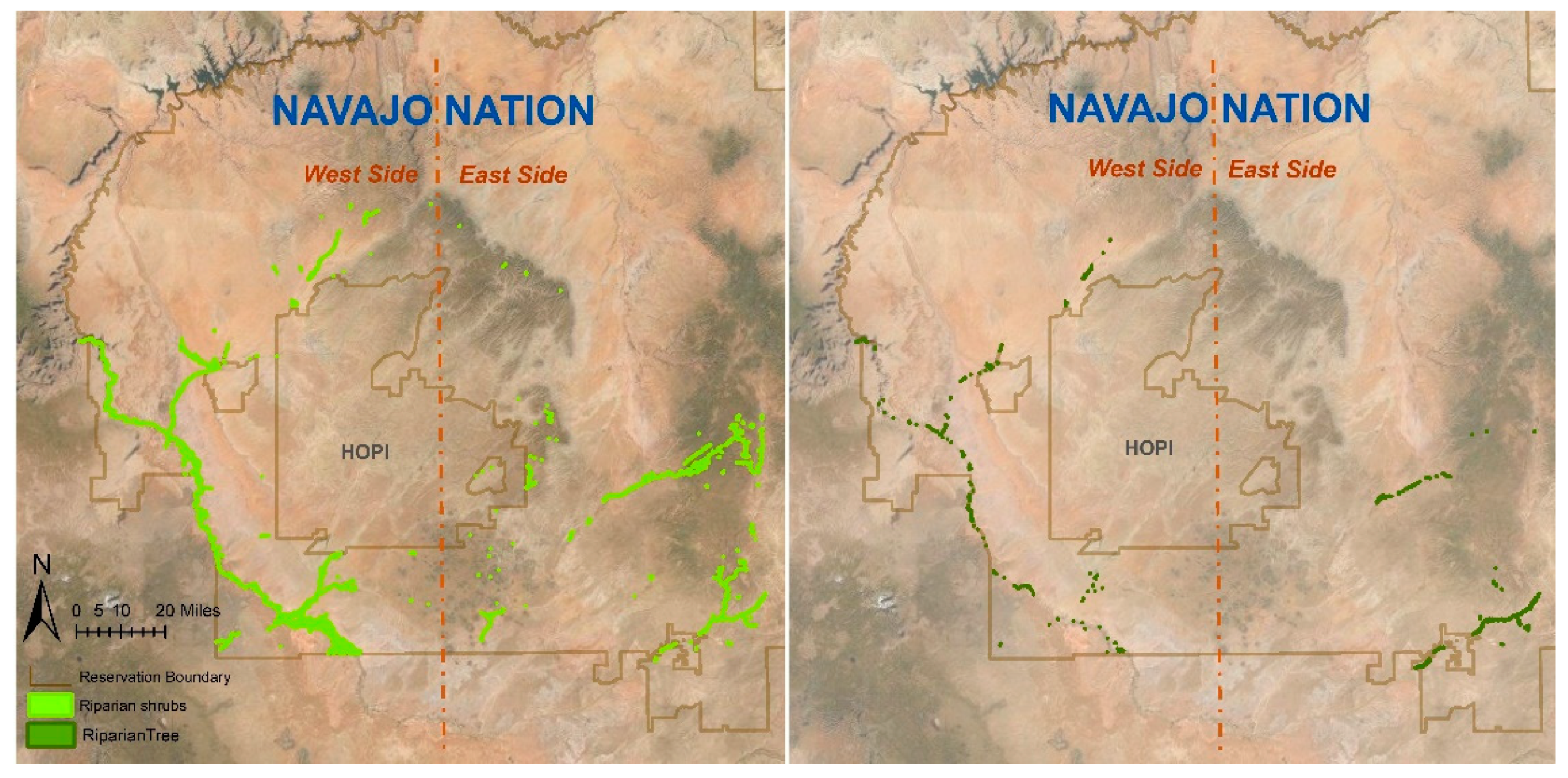
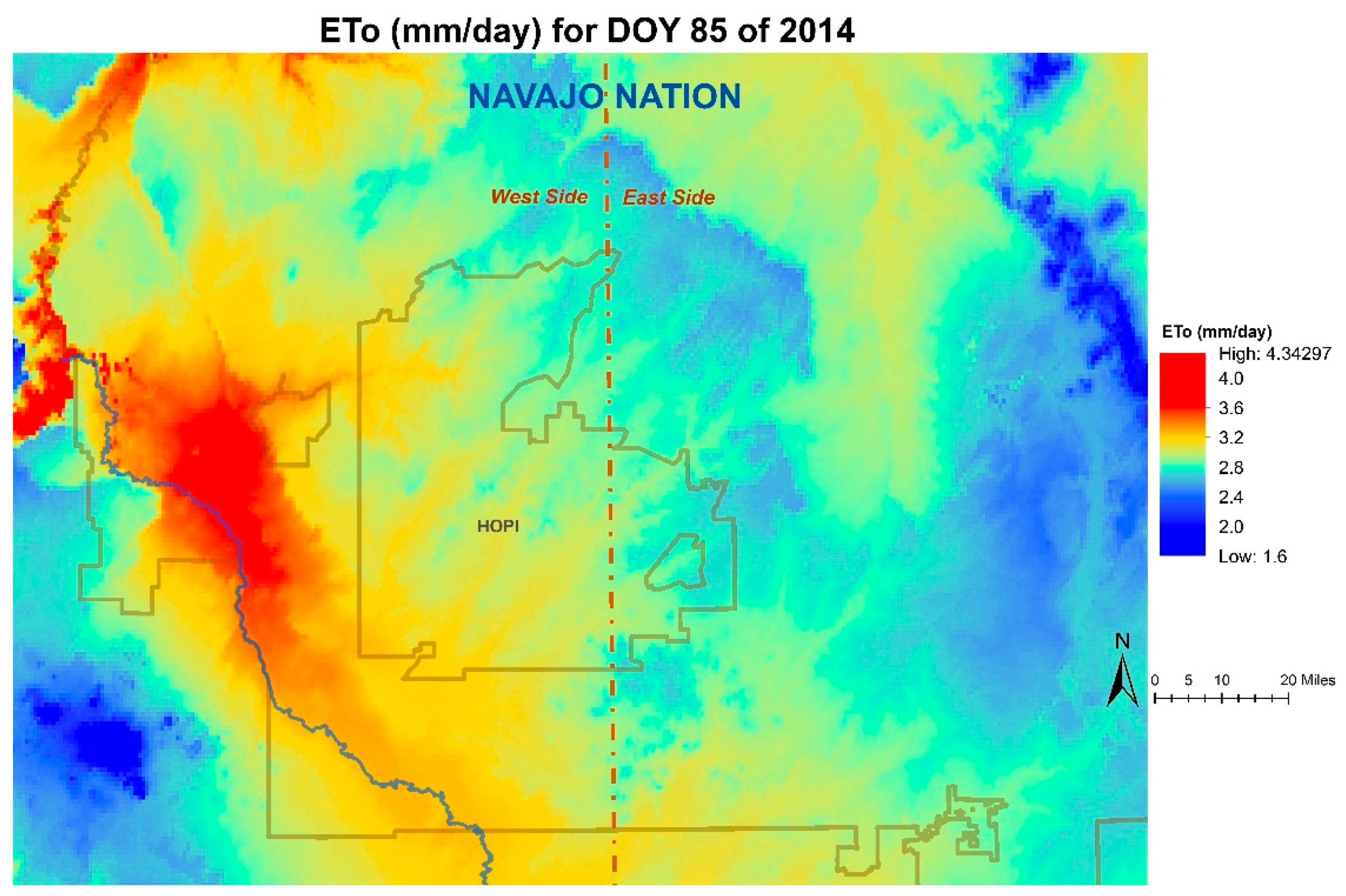
2.6. A West:East Divide for Weather Data on the Navajo Nation
3. Results
3.1. Area Determinations and Literature-Based Estimates
3.2. West:East Divide Based on Physiography and Weather Data across the Navajo Nation
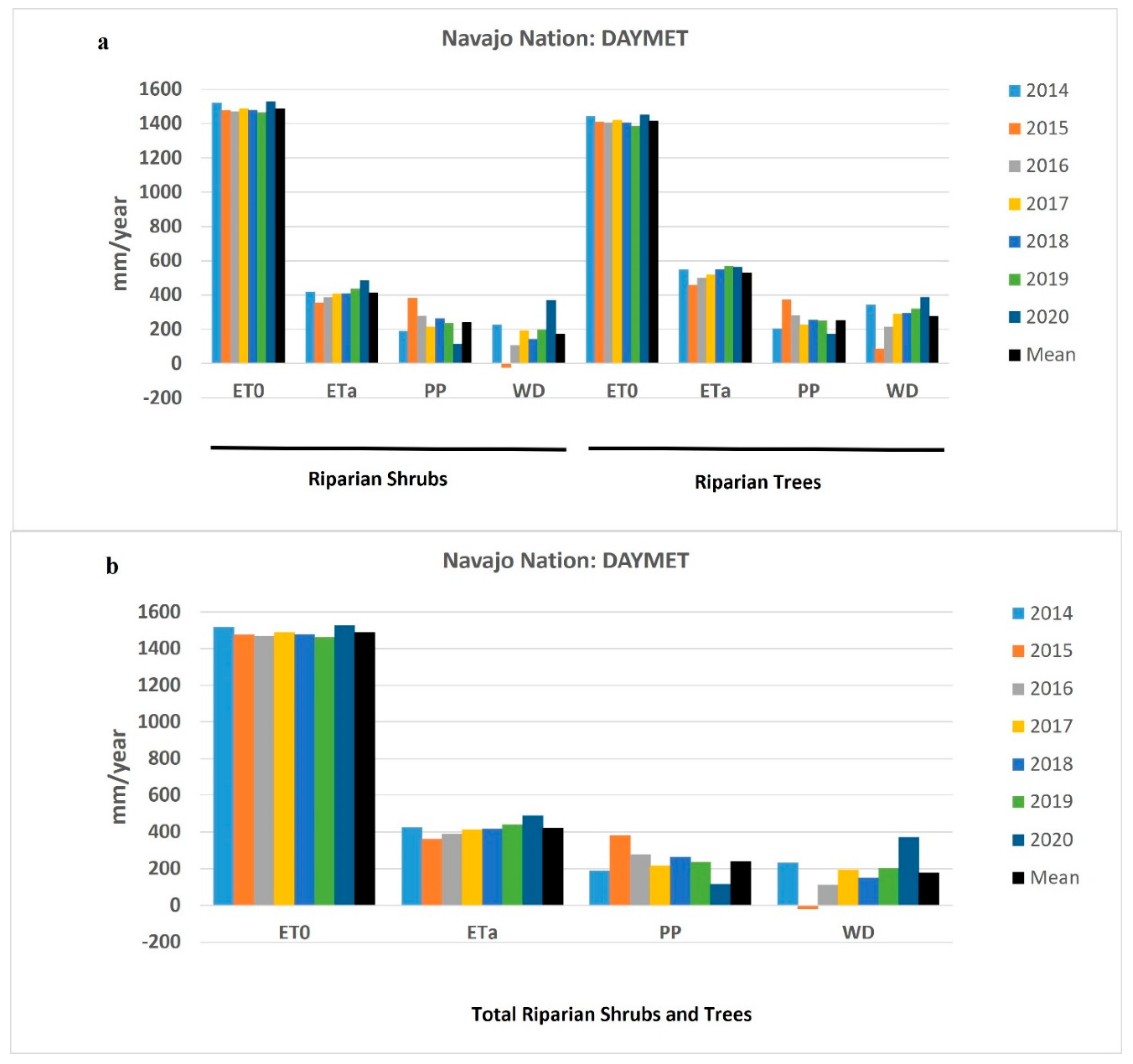
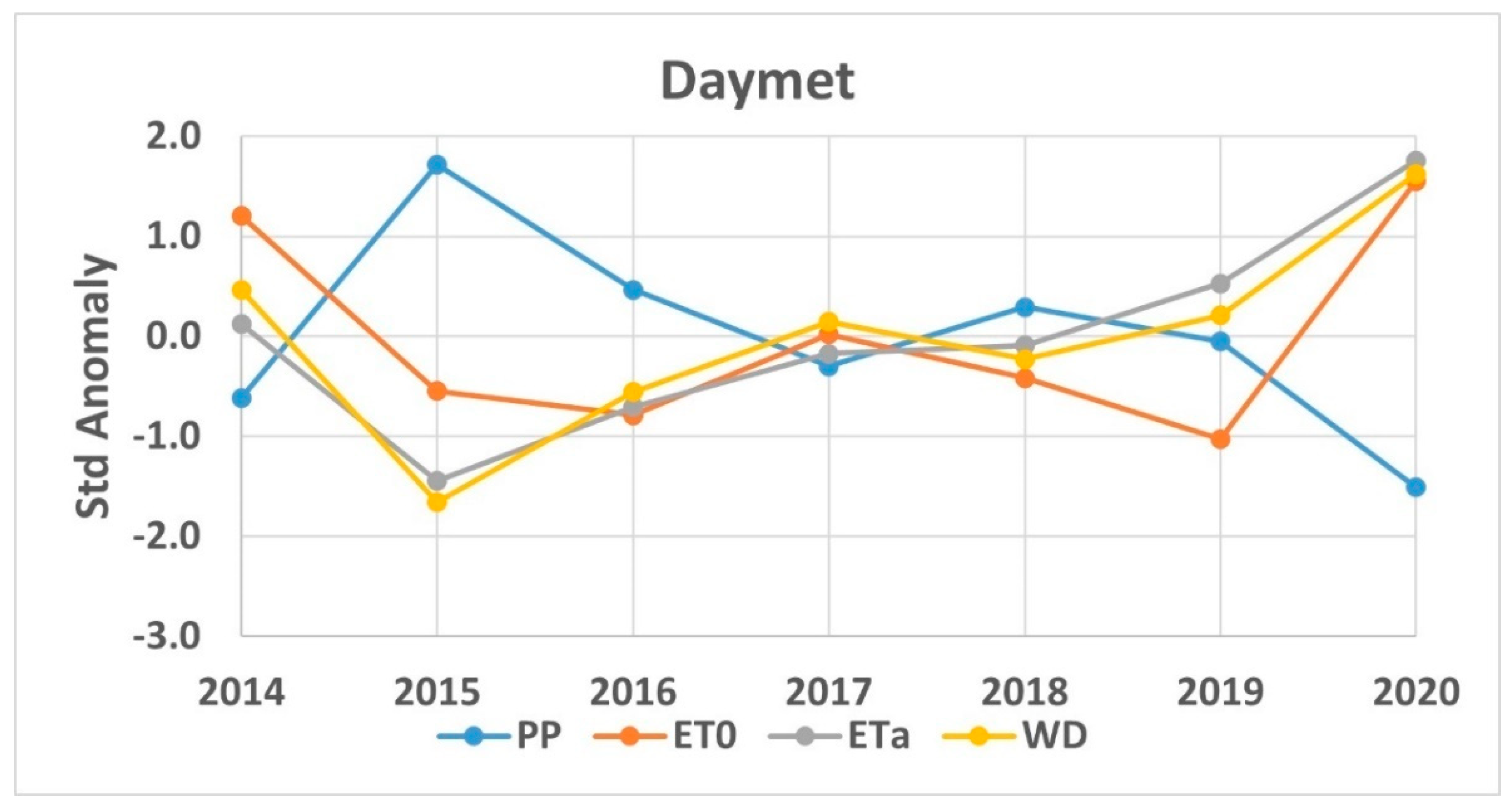
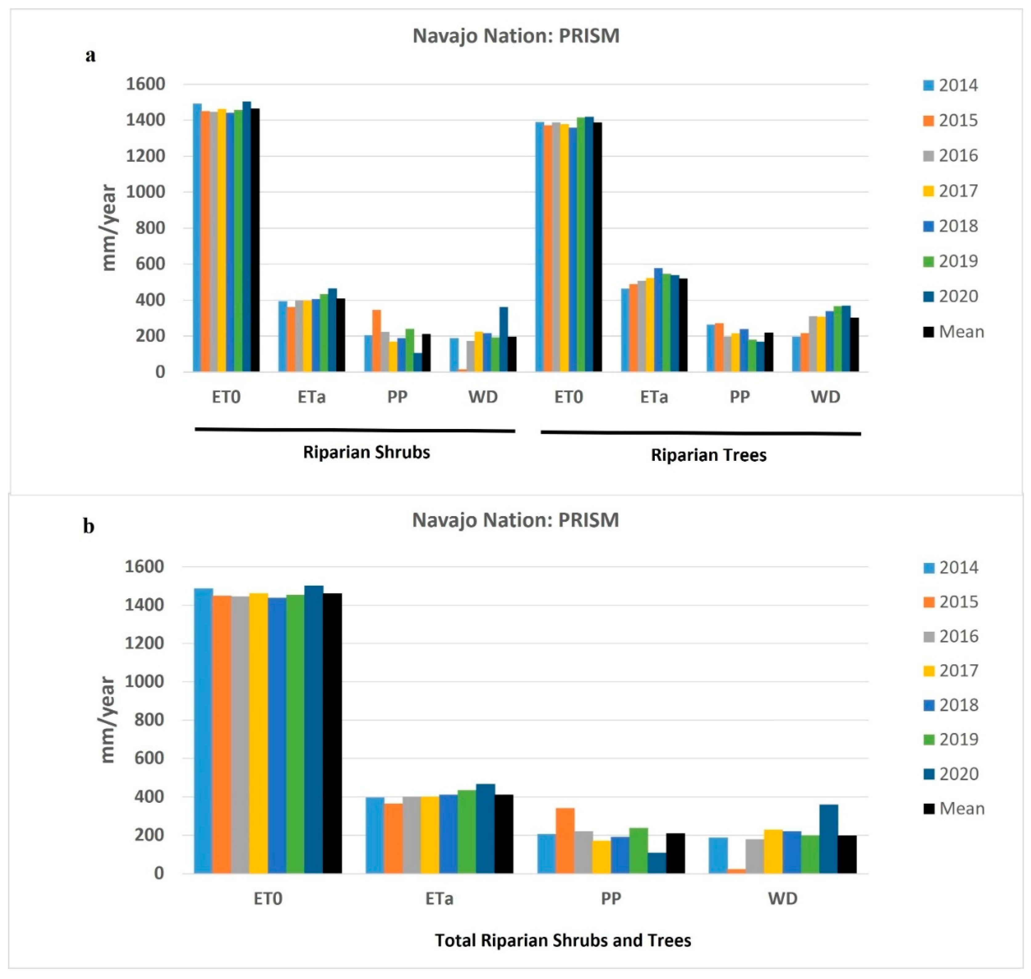
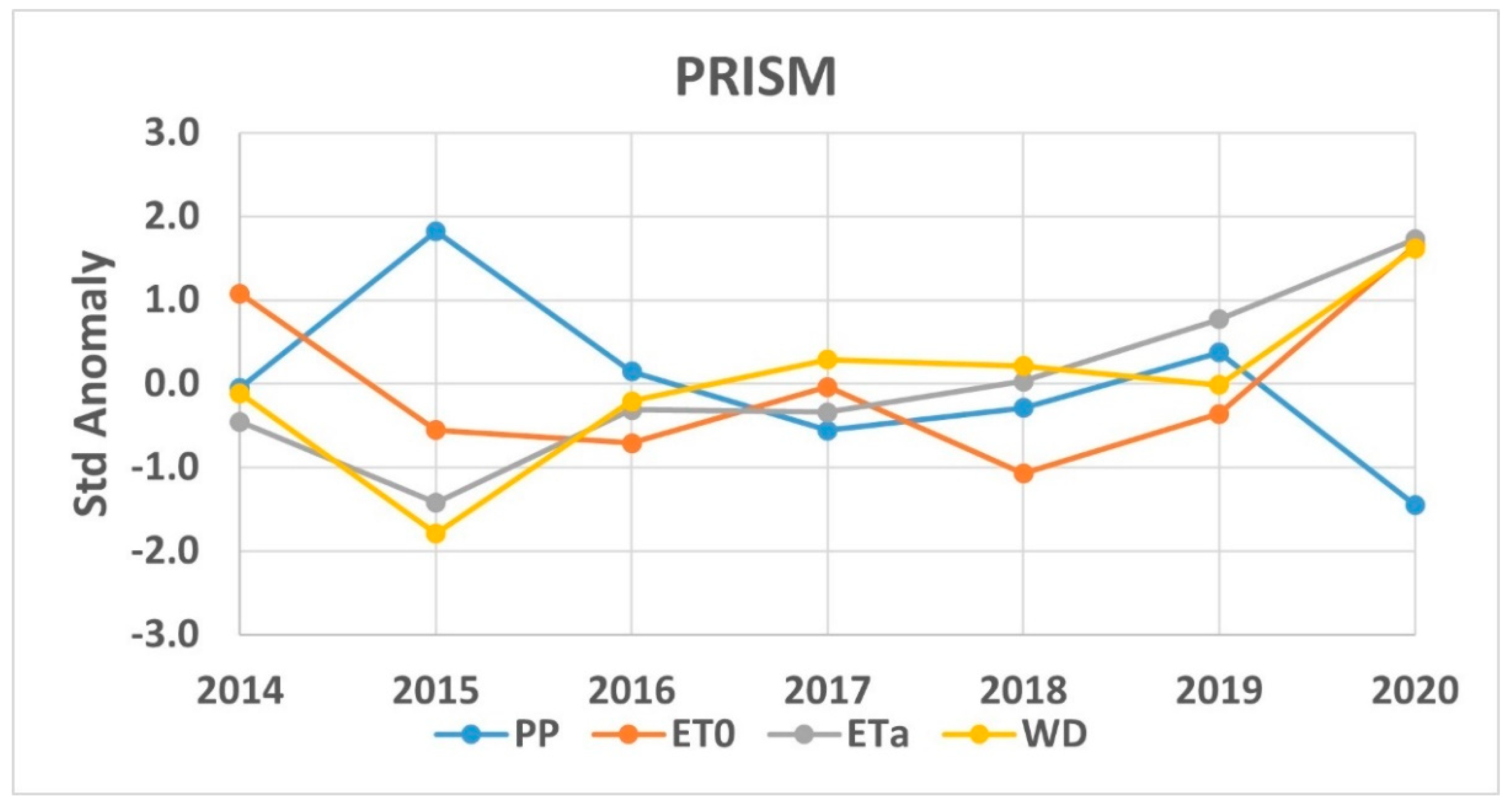
3.3. A Newer Nagler ET(EVI2) Method Based on Landsat and Gridded Weather Data from Daymet and PRISM for Riparian Corridor Water Use Estimation
4. Discussion
4.1. Vegetation Index-Based Evapotranspiration and Consumptive Use Estimation in the Literature
4.2. Riparian Vegetation Consumptive Use by Area
4.3. Quantification of Percent Changes for Ranges of Years
4.4. Limitations
5. Conclusions
Author Contributions
Funding
Institutional Review Board Statement
Informed Consent Statement
Data Availability Statement
Acknowledgments
Conflicts of Interest
References
- Ffolliott, P.F.; Baker, M.B., Jr.; DeBano, L.F.; Neary, D.G. Introduction. In Riparian Areas of the Southwestern United States: Hydrology, Ecology and Management; Baker, M.B., Jr., Ffolliott, P.F., DeBano, L.F., Neary, D.G., Eds.; CRC Press: Boca Raton, FL, USA, 2004; pp. 1–9. [Google Scholar]
- Zaimes, G.; Nichols, M.; Green, D.; Crimmins, M. Defining Arizona’s Riparian Areas and their Importance to the Landscape, Characterization of Riparian Areas, Hydrologic and Stream Processes in Riparian Areas. In Understanding Arizona’s Riparian Areas; College of Agriculture and Life Sciences, University of Arizona: Tucson, AZ, USA, 2007; pp. 1–54. Available online: https://repository.arizona.edu/handle/10150/146921 (accessed on 12 December 2022).
- Rood, S.B.; Goater, L.A.; Mahoney, J.M.; Pearce, C.M.; Smith, D.G. Floods, fire, and ice: Disturbance ecology of riparian cottonwoods. Botany 2007, 85, 1019–1032. [Google Scholar]
- Loheide, S.P.; Booth, E.G. Effects of changing channel morphology on vegetation, groundwater, and soil moisture regimes in groundwater-dependent ecosystems. Geomorphology 2011, 126, 364–376. [Google Scholar] [CrossRef]
- Nagler, P.L.; Pearlstein, S.; Glenn, E.P.; Brown, T.B.; Bateman, H.L.; Bean, D.W.; Hultine, K.R. Rapid dispersal of saltcedar (Tamarix spp.) biocontrol beetles (Diorhabda carinulata) on a desert river detected by phenocams, MODIS imagery and ground observations. Remote Sens. Environ. 2014, 140, 206–219. [Google Scholar] [CrossRef]
- Singh, R.K.; Senay, G.B.; Velpuri, N.M.; Bohms, S.; Scott, R.L.; Verdin, J.P. Actual Evapotranspiration (Water Use) Assessment of the Colorado River Basin at the Landsat Resolution Using the Operational Simplified Surface Energy Balance Model. Remote Sens. 2014, 6, 233–256. [Google Scholar] [CrossRef] [Green Version]
- Nagler, P.L.; Barreto-Muñoz, A.; Chavoshi Borujeni, S.; Nouri, H.; Jarchow, C.J.; Didan, K. Riparian area changes in greenness and water use on the Lower Colorado River in the USA from 2000–2020. Remote Sens. 2021, 13, 1332. [Google Scholar] [CrossRef]
- Loheide II, S.P.; Gorelick, S.M. A local-scale, high-resolution evapotranspiration mapping algorithm (ETMA) with hydroecological applications at riparian meadow restoration sites. Remote Sens. Environ. 2005, 98, 182–200. [Google Scholar] [CrossRef]
- Yang, H.; Rood, S.B.; Flanagan, L.B. Controls on ecosystem water-use and water-use efficiency: Insights from a comparison between grassland and riparian forest in the northern Great Plains. Agric. For. Meteorol. 2019, 271, 22–32. [Google Scholar] [CrossRef]
- Loheide, S.P.; Gorelick, S.M. Riparian hydroecology: A coupled model of the observed interactions between groundwater flow and meadow vegetation patterning. Water Resour. Res. 2007, 43, W07414. [Google Scholar] [CrossRef]
- Flanagan, L.B.; Orchard, T.E.; Logie, G.S.; Coburn, C.A.; Rood, S.B. Water use in a riparian cottonwood ecosystem: Eddy covariance measurements and scaling along a river corridor. Agric. For. Meteorol. 2017, 232, 332–348. [Google Scholar] [CrossRef]
- Flanagan, L.B.; Orchard, T.E.; Tremel, T.N.; Rood, S.B. Using stable isotopes to quantify water sources for trees and shrubs in a riparian cottonwood ecosystem in flood and drought years. Hydrol. Process. 2019, 33, 3070–3083. [Google Scholar] [CrossRef]
- Lurtz, M.R.; Morrison, R.R.; Gates, T.K.; Senay, G.B.; Bhaskar, A.S.; Ketchum, D.G. Relationships between riparian evapotranspiration and groundwater depth along a semiarid irrigated river valley. Hydrol. Process. 2020, 34, 1714–1727. [Google Scholar] [CrossRef]
- Breshears, D.D.; Myers, O.B.; Meyer, C.F.; Barnes, F.J.; Zou, C.B.; Allen, C.D.; McDowell, N.G.; Pockman, W.T. Tree die-off in response to global change-type drought: Mortality insights from a decade of plant water potential measurements. Front. Ecol. Environ. 2009, 7, 185–189. [Google Scholar] [CrossRef] [Green Version]
- Seager, R.; Ting, M.; Held, I.; Kushnir, Y.; Lu, J.; Vecchi, G.; Huang, H.P.; Harnik, N.; Leetmaa, A.; Lau, N.C.; et al. Model projections of an imminent transition to a more arid climate in southwestern North America. Science 2007, 316, 1181–1184. [Google Scholar] [CrossRef] [PubMed]
- Stevens, L.E.; Meretsky, V.J. Aridland Springs in North America Ecology and Conservation; University of Arizona Press and The Arizona-Sonora Desert Museum: Tucson, AZ, USA, 2008; p. 432. [Google Scholar]
- Stevens, L.E.; Jenness, J.; Ledbetter, J.D. Springs and Springs-Dependent Taxa of the Colorado River Basin, Southwestern North America: Geography, Ecology and Human Impacts. Water 2020, 12, 1501. [Google Scholar] [CrossRef]
- Gribovszki, Z.; Kalicz, P.; Szilagyi, J.; Kucsara, M. Riparian zone evapotranspiration estimation from diurnal groundwater level fluctuations. J. Hydrol. 2008, 349, 6–17. [Google Scholar] [CrossRef]
- Khand, K.; Taghvaeian, S.; Hassan-Esfahani, L. Mapping annual riparian water use based on single-satellite-scene approach. Remote Sens. 2017, 9, 832. [Google Scholar] [CrossRef] [Green Version]
- Jensen, M.E.; Burman, R.D.; Allen, R.G. Evapotranspiration and Irrigation Water Requirements. In ASCE Manuals and Reports on Engineering Practice No. 70; American Society of Civil Engineers (ASCE): New York, NY, USA, 1990. [Google Scholar]
- Allen, R.; Pereira, L.; Rais, D.; Smith, M. Crop Evapotranspiration—Guidelines for Computing Crop Water Requirements—FAO Irrigation and Drainage Paper 56; Food and Agriculture Organization of the United Nations: Rome, Italy, 1998. [Google Scholar]
- Nagler, P.; Scott, R.; Westenburg, C.; Cleverly, J.; Glenn, E.; Huete, A. Evapotranspiration on western U.S. rivers estimated using the Enhanced Vegetation Index from MODIS and data from eddy covariance and Bowen ratio flux towers. Remote Sens. Environ. 2005, 97, 337–351. [Google Scholar] [CrossRef]
- Nagler, P.L.; Glenn, E.P.; Kim, H.; Emmerich, W.; Scott, R.L.; Huxmam, T.E.; Huete, A.R. Relationship between evapotranspiration and precipitation pulses in a semiarid rangeland estimated by moisture flux towers and MODIS vegetation indices. J. Arid Environ. 2007, 70, 443–462. [Google Scholar] [CrossRef]
- Nagler, P.; Jetton, A.; Fleming, J.; Didan, K.; Glenn, E.; Erker, J.; Morino, K.; Milliken, J.; Gloss, S. Evapotranspiration in a cottonwood (Populus fremontii) restoration plantation estimated by sap flow and remote sensing methods. Agric. For. Meteoro. 2007, 144, 95–110. [Google Scholar] [CrossRef]
- Nagler, P.L.; Morino, K.; Didan, K.; Osterberg, J.; Hultine, K.; Glenn, E. Wide-area estimates of saltcedar (Tamarix spp.) evapotranspiration on the lower Colorado River measured by heat balance and remote sensing methods. Ecohydrology 2009, 2, 18–33. [Google Scholar] [CrossRef]
- Jensen, M.E. Coefficients for Vegetative Evapotranspiration and Open Water Evaporation for the Lower Colorado River Accounting System; United States Bureau of Reclamation, Boulder Canyon Operations Office: Boulder City, NV, USA, 1998. [Google Scholar]
- USBR, United States Bureau of Reclamation; LCRAS, Lower Colorado River Accounting System. Evapotranspiration and Evaporation Calculations, Calendar Year 2007; United States Bureau of Reclamation: Boulder City, NV, USA, 2008. [Google Scholar]
- Nagler, P.; Glenn, E.P.; Hursh KCurtis, C. Vegetation Mapping for Change Detection on an Arid-Zone River. Environ Monit Assess. 2005, 109, 255–274. [Google Scholar] [CrossRef] [PubMed]
- Nagler, P.L.; Glenn, E.P.; Hinojosa-Huerta, O.; Zamora, F.; Howard, K. Riparian vegetation dynamics and evapotranspiration in the riparian corridor in the delta of the Colorado River, Mexico. J. Environ. Manage. 2008, 88, 864–874. [Google Scholar] [CrossRef] [PubMed]
- Nagler, P.L.; Murray, R.S.; Morino, K.; Osterberg, J.; Glenn, E.P. Scaling riparian and agricultural evapotranspiration in river irrigation districts based on potential evapotranspiration, ground measurements of actual evapotranspiration, and the Enhanced Vegetation Index from MODIS. I. Description of method. Remote Sens. 2009, 1, 1273–1297. [Google Scholar] [CrossRef] [Green Version]
- Murray, R.S.; Nagler, P.L.; Morino, K.; Glenn, E.P. An empirical algorithm for estimating agricultural and riparian evapotranspiration using MODIS Enhanced Vegetation Index and ground measurements of ET. II. Application to the Lower Colorado River, U.S. Remote Sens. 2009, 1, 1125–1138. [Google Scholar] [CrossRef] [Green Version]
- Nagler, P.L. Literature-Reviewed Estimates of Riparian Consumptive Water Use in the Drylands of Northeast Arizona, USA. In U.S. Geological Survey Open-File Report 2020–1129; U.S. Geological Survey: Flagstaff, AZ, USA, 2020; p. 9. [Google Scholar] [CrossRef]
- AZMET. The Arizona Meteorological Network; University of Arizona: Tucson, AZ, USA; Available online: http://cals.arizona.edu/azmet/ (accessed on 12 December 2022).
- Nagler, P.L.; Barreto-Muñoz, A.; Chavoshi Borujeni, S.; Jarchow, C.J.; Gómez-Sapiens, M.M.; Nouri, H.; Herrmann, S.M.; Didan, K. Ecohydrological responses to surface flow across borders: Two decades of changes in vegetation greenness and water use in the riparian corridor of the Colorado River delta. Hydrol. Process. 2020, 34, 4851–4883. [Google Scholar] [CrossRef]
- Hunsaker, D.J.; Pinter, P.J.; Cai, H. Alfalfa basal crop coefficients for FAO–56 procedures in the desert regions of the southwestern US. Trans. ASAE 2002, 45, 1799–1815. [Google Scholar] [CrossRef]
- Thornton, M.M.; Thornton, P.E.; Wei, Y.; Mayer, B.W.; Cook, R.B.; Vose, R.S. Daymet: Monthly Climate Summaries on a 1-km Grid for North America, Version 4; ORNL DAAC: Oak Ridge, TN, USA, 2020. [Google Scholar] [CrossRef]
- Daymet: Daily Surface Weather and Climatological Summaries. Available online: https://daymet.ornl.gov/ (accessed on 25 July 2022).
- Daly, C.; Taylor, G.H.; Gibson, W.P.; Parzybok, T.W.; Johnson, G.L.; Pasteris, P.A. High-quality spatial climate data sets for the United States and beyond. Trans. ASAE 2000, 43, 1957. [Google Scholar] [CrossRef] [Green Version]
- Daly, C.; Halbleib, M.; Smith, J.I.; Gibson, W.P.; Doggett, M.K.; Taylor, G.H.; Curtis, J.; Pasteris, P.P. Physiographically sensitive mapping of climatological temperature and precipitation across the conterminous United States. Int. J. Climatol. A J. R. Meteorol. Soc. 2008, 28, 2031–2064. [Google Scholar] [CrossRef]
- PRISM, Parameter-elevation Relationships on Independent Slopes Model. 2008. Available online: https://prism.oregonstate.edu/recent/ (accessed on 25 July 2022).
- Colorado State University, Colorado Water Knowledge, Water Uses. Available online: https://waterknowledge.colostate.edu/water-management-administration/water-uses/ (accessed on 12 December 2022).
- Maupin, M.A.; Ivahnenko, T.I.; Bruce, B. Estimates of Water Use and Trends in the Colorado River Basin, Southwestern United States, 1985–2010; SIR 2018–5049; U.S. Geological Survey: Flagstaff, AZ, USA, 2018. [Google Scholar] [CrossRef]
- PHSR, Hopi Preliminary Hydrographic Survey Report; Arizona Department of Water Resources: Phoenix, AZ, USA, 2008.
- Shirley, S.J.; Shelly, P.B. The Navajo Nation Executive Branch; Department of Dine Education, Navajo Nation: Window Rock, AZ, USA; Arizona Department of Water Resources: Phoenix, AZ, USA, 2010. [Google Scholar]
- NRCE, Natural Resources Consulting Engineers. Hopi Indian Reservation Riparian and Wetland Habitat Water Use Pasture Canyon; U.S. Dept. of Justice, Environmental & Natural Resources Division: Denver, CO, USA, 2017. [Google Scholar]
- USBR, U.S.; Bureau of Reclamation. Colorado River Basin Water Supply and Demand Study. 2012. Available online: https://www.usbr.gov/lc/region/programs/crbstudy/finalreport/Executive%20Summary/Executive_Summary_FINAL_Dec2012.pdf (accessed on 25 July 2022).
- NAIP, National Agriculture Imagery Program, The USGS EROS Archive, Aerial Photography. Available online: https://www.usgs.gov/centers/eros/science/usgs-eros-archive-aerial-photography-national-agriculture-imagery-program-naip (accessed on 12 December 2022).
- Jiang, Z.; Huete, A.; Didan, K.; Miura, T. Development of a two-band enhanced vegetation index without a blue band. Remote Sens. Environ. 2008, 112, 3833–3845. [Google Scholar] [CrossRef]
- Huete, A.R.; Miura, T.; Kim, Y.; Didan, K.; Privette, J.P. Assessments of multisensor vegetation index dependencies with hyperspectral and tower flux data. In Proceedings of the SPIE 6298, Remote Sensing and Modeling of Ecosystems for Sustainability III, San Diego, CA, USA, 27 September 2006; Volume 6298, p. 629814. [Google Scholar] [CrossRef]
- Didan, K.; Barreto-Muñoz, A.; Solano, R.; Huete, A. MODIS Vegetation Index User’s Guide (MOD13 Series) Vegetation Index and Phenology Lab; The University of Arizona: Tucson, AZ, USA, 2015; pp. 1–38. Available online: https://vip.arizona.edu/MODIS_UsersGuide.php (accessed on 12 December 2022).
- Allen, R.G.; Pereira, L.S.; Howell, T.A.; Jensen, M.E. Evapotranspiration information reporting: I. Factors governing measurement accuracy. Agric. Water Manag. 2011, 98, 899–920. [Google Scholar] [CrossRef] [Green Version]
- Blaney, H.F.; Criddle, W.D. Determining water needs from climatological data. In USDA Soil Conservation Service; SOS–TP: USA, 1950; pp. 8–9. [Google Scholar]
- FAO, United Nations Food and Agricultural Organization. Irrigation Water Management: Irrigation Water Needs, 1986, Chapter 3, Crop Water Needs. Available online: https://www.fao.org/3/s2022e/s2022e07.htm#3.1.3%20blaney%20criddle%20method (accessed on 12 December 2022).
- NOAA, National Oceanic and Atmospheric Administration, NCEI, National Centers for Environmental Information. Available online: https://www.ncei.noaa.gov/ (accessed on 12 December 2022).
- Nagler, P.L.; Glenn, E.P.; Nguyen, U.; Scott, R.L.; Doody, T. Estimating Riparian and Agricultural Actual Evapotranspiration by Reference Evapotranspiration and MODIS Enhanced Vegetation Index. Remote Sens. 2013, 5, 3849–3871. [Google Scholar] [CrossRef] [Green Version]
- Huete, A.; Didan, K.; Miura, T.; Rodriguez, E.P.; Gao, X.; Ferreira, L.G. Overview of the radiometric and biophysical performance of the MODIS vegetation indices. Rem. Sens. Environ. 2002, 83, 195–213. [Google Scholar] [CrossRef]
- Huete, A.R.; Glenn, E.P. Remote sensing of ecosystem structure and function. In Advances in Environmental Remote Sensing; Sensors, Algorithms, and Applications; CRC Press: Boca Raton, FL, USA, 2011; pp. 291–320. [Google Scholar]
- Jarchow, C.J.; Nagler, P.L.; Glenn, E.P. Greenup and evapotranspiration following the Minute 319 pulse flow to Mexico: An analysis using Landsat 8 Normalized Difference Vegetation Index (NDVI) data. Ecol. Eng. 2017, 106, 776–783. [Google Scholar] [CrossRef]
- Jarchow, C.J.; Nagler, P.L.; Glenn, E.P.; Ramírez-Hernández, J.; Rodríguez-Burgueno, J.E. Evapotranspiration by remote sensing: An analysis of the Colorado River Delta before and after the Minute 319 pulse flow to Mexico. Ecol. Eng. 2017, 106, 725–732. [Google Scholar] [CrossRef]
- Jarchow, C.J.; Didan, K.; Barreto-Muñoz, A.; Nagler, P.L.; Glenn, E.P. Application and Comparison of the MODIS-Derived Enhanced Vegetation Index to VIIRS, Landsat 5 TM and Landsat 8 OLI Platforms: A Case Study in the Arid Colorado River Delta, Mexico. Sensors 2018, 18, 1546. [Google Scholar] [CrossRef] [PubMed] [Green Version]
- Ponce-Campos, G.E.; Moran, M.S.; Huete, A.; Zhang, Y.; Bresloff, C.; Huxman, T.E.; Eamus, D.; Bosch, D.D.; Buda, A.R.; Gunter, S.A.; et al. Ecosystem resilience despite large-scale altered hydroclimatic conditions. Nature 2013, 494, 349–352. [Google Scholar] [CrossRef] [PubMed]
- Nagler, P.L.; Barreto-Muñoz, A.; Sall, I.; Didan, K. Uncultivated Plant Water Use (Riparian Evapotranspiration) and Consumptive Use Data for Selected Areas of the Little Colorado River Watershed on the Navajo Nation, Arizona. U.S. Geological Survey Data Release; 2022. Available online: https://www.usgs.gov/data/uncultivated-plant-water-use-riparian-evapotranspiration-and-consumptive-use-data-selected (accessed on 12 December 2022).
- Senay, G.B.; Friedrichs, M.; Morton, C.; Parrish, G.E.; Schauer, M.; Khand, K.; Kagone, S.; Boiko, O.; Huntington, J. Mapping actual evapotranspiration using Landsat for the conterminous United States: Google Earth Engine implementation and assessment of the SSEBop model. Rem. Sens. Environ. 2022, 275, 113011. [Google Scholar] [CrossRef]
- Melton, F.S.; Huntington, J.; Grimm, R.; Herring, J.; Hall, M.; Rollison, D.; Erickson, T.; Allen, R.; Anderson, M.; Fisher, J.B.; et al. Openet: Filling a critical data gap in water management for the western united states. JAWRA J. Am. Water Resour. Assoc. 2021, 1–24. [Google Scholar] [CrossRef]
- Fisher, J.B.; Lee, B.; Purdy, A.J.; Halverson, G.H.; Dohlen, M.B.; Cawse-Nicholson, K.; Wang, A.; Anderson, R.G.; Aragon, B.; Arain, M.A.; et al. ECOSTRESS: NASA’s next generation mission to measure evapotranspiration from the international space station. Water Resour. Res. 2020, 56, e2019WR026058. [Google Scholar] [CrossRef]
- McVicar, T.; Vleeshouwer, J.; Van Niel, T.; Guerschman, J. Actual Evapotranspiration for Australia using CMRSET algorithm. Terrestrial Ecosystem Research Network. Dataset 2022. [Google Scholar] [CrossRef]
- Glenn, E.P.; Doody, T.M.; Guerschman, J.P.; Huete, A.R.; King, E.A.; Mcvicar, T.R.; Van Dijk, A.I.J.M.; Van Niel, T.G.; Yebra, M.; Zhang, Y. Actual evapotranspiration estimation by ground and remote sensing methods: The Australian experience. Hydrological Processes 2011, 25, 4103–4116. [Google Scholar] [CrossRef]
- Guerschman, J.P.; Van Dijk, A.I.; Mattersdorf, G.; Beringer, J.; Hutley, L.B.; Leuning, R.; Pipunic, R.C.; Sherman, B.S. Scaling of potential evapotranspiration with MODIS data reproduces flux observations and catchment water balance observations across Australia. J. Hydrol. 2009, 369, 107–119. [Google Scholar] [CrossRef]
- Abbasi, N.; Nouri, H.; Didan, K.; Barreto-Muñoz, A.; Chavoshi Borujeni, S.; Salemi, H.; Opp, C.; Siebert, S.; Nagler, P. Estimating Actual Evapotranspiration over Croplands Using Vegetation Index Methods and Dynamic Harvested Area. Remote Sensing 2021, 13, 5167. [Google Scholar] [CrossRef]
- Hunsaker, D.J.; Fitzgerald, G.J.; French, A.N.; Clarke, T.R.; Ottman, M.J.; Pinter, P.J. Wheat irrigation management using multispectral crop coefficients. I. Crop evapotranspiration prediction. Trans. ASAE 2007, 50, 2017–2033. [Google Scholar] [CrossRef]
- French, A.N.; Hunsaker, D.J.; Sanchez, C.A.; Saber, M.; Gonzalez, J.R.; Anderson, R. Satellite-based NDVI crop coefficients and evapotranspiration with eddy covariance validation for multiple durum wheat fields in the US Southwest. Agric. Water Manag. 2020, 239, 106266. [Google Scholar] [CrossRef]
- Glenn, E.P.; Neale, C.M.U.; Hunsaker, D.J.; Nagler, P.L. Vegetation index-based crop coefficients to estimate evapotranspiration by remote sensing in agricultural and natural ecosystems. Hydrol. Process. 2011, 25, 4050–4062. [Google Scholar] [CrossRef]
- Glenn, E.; Huete, A.; Nagler, P.L.; Nelson, S.G. Relationship between remotely-sensed vegetation indices, canopy attributes & plant physiological processes: What vegetation indices can and cannot tell us about the landscape. Sensors 2008, 8, 2136–2160. [Google Scholar]
- Huete, A.R.; Didan, K.; van Leeuwen, W.; Miura, T.; Glenn, E.P. MODIS Vegetation Indices. In Land Remote Sensing and Global Environmental Change; Remote Sensing and Digital Image Processing; Ramachandran, B., Justice, C., Abrams, M., Eds.; Springer: New York, NY, USA, 2010; Volume 11. [Google Scholar] [CrossRef]
- Glenn, E.P.; Nagler, P.L.; Huete, A.R. Vegetation index methods for estimating evapotranspiration by remote sensing. Surv. Geophys. 2010, 31, 531–555. [Google Scholar] [CrossRef]
- Jarchow, C.J.; Waugh, W.J.; Didan, K.; Barreto-Muñoz, A.; Herrmann, S.; Nagler, P.L. Vegetation-groundwater dynamics at a former uranium mill site following invasion of a biocontrol agent: A time series analysis of Landsat normalized difference vegetation index data. Hydrol. Process. 2020, 34, 2739–2749. [Google Scholar] [CrossRef]
- Jamison, L.R.; Johnson, M.J.; Bean, D.W.; van Riper, C. Phenology and Abundance of Northern Tamarisk Beetle, Diorhabda carinulata Affecting Defoliation of Tamarix. Southwest. Entomol. 2018, 43, 571–584. [Google Scholar] [CrossRef]
- Nagler, P.L.; Nguyen, U.; Bateman, H.L.; Jarchow, C.J.; Glenn, E.P.; Waugh, W.J.; van Riper III, C. Northern tamarisk beetle (Diorhabda carinulata) and tamarisk (Tamarix spp.) interactions in the Colorado River basin. Restor. Ecol. 2018, 26, 348–359. [Google Scholar] [CrossRef]
- McDaniel, K.C.; Bunting, D.P. Controlling Tamarisk Monocultures at the Bosque Del Apache National Wildlife Ref-uge: Lessons Along the Middle Rio Grande, New Mexico. In Renewing Our Rivers: Stream Corridor Restoration in Dryland Regions; University of Arizona Press: Tucson, AZ, USA, 2021; p. 244. [Google Scholar]
- Nagler, P.L.; Sall, I.; Barreto-Muñoz, A.; Gómez-Sapiens, M.; Nouri, H.; Chavoshi Borujeni, S.; Didan, K. Effect of restoration on vegetation greenness and water use in relation to drought in the riparian woodlands of the Colorado River delta. J. Am. Water Resour. Assoc. 2022, 58, 746–784. [Google Scholar] [CrossRef]
- Glenn, E.P.; Morino, K.; Didan, K.; Jordan, F.; Carroll, K.C.; Nagler, P.L.; Hultine, K.; Sheader, L.; Waugh, J. Scaling sap flux measurements of grazed and ungrazed shrub communities with fine and coarse-resolution remote sensing. Ecohydrology 2008, 1, 316–329. [Google Scholar] [CrossRef]
- Bresloff, C.J.; Nguyen, U.; Glenn, E.P.; Waugh, W.J.; Nagler, P.L. Effects of grazing on leaf area index, fractional cover and evapotranspiration by a desert phreatophyte community at a former uranium mill site on the Colorado Plateau. J. Environ. Manag. 2013, 114, 92–104. [Google Scholar] [CrossRef] [PubMed]
- Groeneveld, D.P.; Baugh, W.M.; Sanderson, J.S.; Cooper, D.J. Annual groundwater evapotranspiration mapped from single satellite scenes. J. Hydrol. 2007, 344, 146–156. [Google Scholar] [CrossRef]
- Glenn, E.P.; Jarchow, C.J.; Waugh, W.J. Evapotranspiration dynamics and effects on groundwater recharge and discharge at an arid waste disposal site. J. Arid. Environ. 2016, 133, 1–9. [Google Scholar] [CrossRef] [Green Version]
- Jarchow, C.J.; Waugh, W.J.; Nagler, P.L. Calibration of an evapotranspiration algorithm in a semiarid sagebrush steppe using a 3-ha lysimeter and Landsat normalized difference vegetation index data. Ecohydrology 2022, 15, e2413. [Google Scholar] [CrossRef]
- Tabari, H.; Hosseinzadeh Talaee, P.; Some’e, B.S. Spatial modelling of reference evapotranspiration using adjusted Blaney-Criddle equation in an arid environment. Hydrol. Sci. J. 2013, 58, 408–420. [Google Scholar] [CrossRef]
- Cleverly, J.R.; Dahm, C.N.; Thibault, J.R.; McDonnell, D.E.; Allred Coonrod, J.E. Riparian ecohydrology: Regulation of water flux from the ground to the atmosphere in the Middle Rio Grande, New Mexico. Hydrol. Process. Int. J. 2006, 20, 3207–3225. [Google Scholar] [CrossRef] [Green Version]
- Tillman, F.D.; Callegary, J.B.; Nagler, P.L.; Glenn, E.P. A simple method for estimating basin-scale groundwater discharge by vegetation in the basin and range province of Arizona using remote sensing information and geographic information systems. J. Arid. Environ. 2012, 82, 44–52. [Google Scholar] [CrossRef]
- Long, K.A. Integrating Satellite-Derived Precipitation Measurements to Assess Water Resources on the Navajo Nation and the Four Corners Region. Ph.D. Dissertation, University of Georgia, Athens, GA, USA, 2020. Available online: https://esploro.libs.uga.edu/esploro/outputs/doctoral/Integrating-Satellite-Derived-Precipitation-Measurements-to-Assess-Water-Resources-on-the-Navajo-Nation-and-the-Four-Corners-Region/9949365737402959 (accessed on 12 December 2022).
- Nielsen-Gammon, J.W.; Fipps, G.; Caldwell, T.; McRoberts, D.B.; Conlee, D. Feasibility Study for Development of Statewide Evapotranspiration Network; Final report 1613581995; The Texas Water Development Board: Austin, TX, USA, 2017. [Google Scholar]
- Caldwell, T.; Huntington, J.; Scanlon, B.; Joros, A.; Howard, T. Improving Irrigation Water Use Estimates with Remote Sensing Technologies: A feasibility study for Texas; Final Project Report; Agricultural Water Conservation Grants Texas Water Development Board: Austin, TX, USA, 2017. [Google Scholar]
- Nagler, P.L.; Sall, I.; Barreto-Muñoz, A.; Didan, K.; Abbasi, N.; Nouri, H.; Schauer, M.; Senay, G.B. Evaluation of Two Types of Evapotranspiration Methods in Riparian Vegetation with the Two-Band Enhanced Vegetation Index and SSEBop in Restored and Unrestored Reaches of the Lower Colorado River in the USA. Available online: https://agu2022fallmeeting-agu.ipostersessions.com/default.aspx?s=F9-82-7F-A4-C7-D1-52-AA-CA-DF-37-BD-F5-B5-EF-88 (accessed on 12 December 2022).


| Cycle | 2013 | 2014 | 2015 | 2016 | 2017 | 2018 | 2019 | 2020 |
|---|---|---|---|---|---|---|---|---|
| 1 | 5 | 8 | 11 | 13 | 16 | 3 | 6 | |
| 2 | 21 | 24 | 27 | 29 | 32 | 19 | 22 | |
| 3 | 37 | 40 | 43 | 45 | 48 | 35 | 38 | |
| 4 | 53 | 56 | 59 | 61 | 64 | 51 | ||
| 5 | 69 | 72 | 75 | 77 | 80 | 67 | 70 | |
| 6 | 85 | 88 | 91 | 93 | 96 | 83 | 86 | |
| 7 | 101 | 104 | 107 | 109 | 112 | 99 | 102 | |
| 8 | 117 | 120 | 123 | 125 | 128 | 115 | 118 | |
| 9 | 133 | 136 | 139 | 141 | 144 | 131 | 134 | |
| 10 | 146 | 149 | 152 | 155 | 157 | 160 | 147 | 150 |
| 11 | 162 | 165 | 168 | 171 | 173 | 176 | 163 | 166 |
| 12 | 178 | 181 | 184 | 187 | 189 | 192 | 179 | 182 |
| 13 | 194 | 197 | 200 | 203 | 205 | 208 | 195 | 198 |
| 14 | 210 | 213 | 216 | 219 | 221 | 224 | 211 | 214 |
| 15 | 226 | 229 | 232 | 235 | 240 | 227 | 230 | |
| 16 | 242 | 245 | 248 | 251 | 253 | 256 | 243 | 246 |
| 17 | 258 | 261 | 264 | 267 | 269 | 272 | 259 | 262 |
| 18 | 274 | 277 | 280 | 283 | 285 | 288 | 275 | 278 |
| 19 | 290 | 293 | 296 | 299 | 301 | 304 | 291 | 294 |
| 20 | 306 | 309 | 312 | 315 | 317 | 320 | 307 | |
| 21 | 322 | 325 | 328 | 331 | 333 | 336 | 323 | 326 |
| 22 | 341 | 344 | 347 | 349 | 352 | 339 | 342 | |
| 23 | 354 | 357 | 360 | 363 | 365 | 358 |
| ‘Conservative’ Raster 30 m | ‘Best-Approximation’ Raster 30 m | Digitized Polygons | ||||
|---|---|---|---|---|---|---|
| Western Area | Hectares | Acres | Hectares | Acres | Hectares | Acres |
| Riparian Tree | 119.7 | 295.8 | 240.48 | 594.2 | 40.2 | 99.4 |
| Shrub | 14,978.6 | 37,012.9 | 19,629.81 | 48,506.2 | 3640.2 | 8995.1 |
| Subtotal | 15,098.3 | 37,308.7 | 19,870.29 | 49,100.5 | 3680.4 | 9094.5 |
| Eastern Area | Hectares | Acres | Hectares | Acres | Hectares | Acres |
| Riparian Tree | 447.3 | 1105.3 | 707.0 | 1746.9 | 155.9 | 385.3 |
| Shrub | 3816.8 | 9431.5 | 5037.6 | 12,448.1 | 1137.7 | 2811.3 |
| Subtotal | 4264.1 | 10,536.8 | 5744.5 | 14195.0 | 1293.6 | 3196.6 |
| Total Area | Hectares | Acres | Hectares | Acres | Hectares | Acres |
| Riparian Tree | 567.0 | 1401.1 | 947.4 | 2341.1 | 196.2 | 484.7 |
| Shrub | 18,795.4 | 46,444.4 | 24,667.4 | 60,954.3 | 4777.9 | 11,806.4 |
| Total | 19,362.4 | 47,845.5 | 25,614.8 | 63,295.5 | 4974.0 | 12,291.1 |
| Riparian Vegetation Type | ETo or ETa (mm/Year) | ETo or ETa (in/Year) | Rainfall (in/Year) *Bresloff et al., 2013 | Net Water Requirement (in/Year) (No Soil Moisture Change) | ETo or ETa (ft/ Year) | Net Water Requirement (ft) | Area (Acres) | Consumptive Water Use (Acre-ft) |
|---|---|---|---|---|---|---|---|---|
| Average Riparian Cover Reach Level | 684 | 26.93 | 6.06 | 20.87 | 2.24 | 1.74 | 14,598 | 25,387 |
| Riparian Gallery Trees Only | 1123 | 44.21 | 6.06 | 38.14 | 3.68 | 3.18 | 14,598 | 46,397 |
| Navajo Nation Potential ET (ETo) | 1473 | 57.99 | 6.06 | 51.93 | 4.83 | 4.33 | 14,598 | 63,258 |
| Lower Colorado River, Potential ET (ETo) | 2021 | 79.57 | 6.06 | 73.51 | 6.63 | 6.13 | 14,598 | 89,486 |
| NRCE Report | 1273 | 50.1 | 5.10 | 45.0 | 4.18 | 3.75 | 26.2 | 98.4 |
| NRCE Report Potential ET (ETo) | 2080 | 81.9 | 8.1 | 73.8 | 6.83 | 6.15 | - | 108.2 |
| West | DAYMET Dataset | |||||||||||
|---|---|---|---|---|---|---|---|---|---|---|---|---|
| Shrub (mm/Year) | Riparian (mm/Year) | Total (mm/Year) | ||||||||||
| Year | ET0 | ETa | PP | WD | ET0 | ETa | PP | WD | ET0 | ETa | PP | WD |
| 2014 | 1561.4 | 409.4 | 174.3 | 235.1 | 1564.1 | 596.9 | 163.8 | 433.1 | 1560.7 | 411.7 | 174.2 | 237.5 |
| 2015 | 1515.0 | 354.1 | 358.2 | −4.1 | 1513.3 | 542.3 | 388.1 | 154.2 | 1513.4 | 356.4 | 358.5 | −2.1 |
| 2016 | 1506.9 | 378.8 | 269.0 | 109.9 | 1515.4 | 542.4 | 303.7 | 238.7 | 1506.3 | 380.8 | 269.4 | 111.4 |
| 2017 | 1524.4 | 383.5 | 200.6 | 182.9 | 1531.5 | 554.0 | 259.0 | 295.0 | 1526.2 | 385.6 | 201.3 | 184.3 |
| 2018 | 1518.0 | 392.6 | 264.0 | 128.6 | 1521.7 | 628.2 | 266.2 | 362.0 | 1517.5 | 395.5 | 264.1 | 131.4 |
| 2019 | 1502.8 | 416.6 | 210.3 | 206.3 | 1504.5 | 558.1 | 217.7 | 340.4 | 1505.1 | 418.3 | 210.4 | 208.0 |
| 2020 | 1568.7 | 476.0 | 92.0 | 384.0 | 1576.3 | 595.8 | 90.4 | 505.3 | 1568.1 | 477.4 | 92.0 | 385.4 |
| Mean | 1528.2 | 401.6 | 224.1 | 177.5 | 1532.4 | 573.9 | 241.3 | 332.7 | 1528.2 | 403.7 | 224.3 | 179.4 |
| Stdev | 26.3 | 38.7 | 83.9 | 120.2 | 27.3 | 33.2 | 96.3 | 117.6 | 25.8 | 38.4 | 84.0 | 120.1 |
| East | DAYMET Dataset | |||||||||||
| Shrub (mm/Year) | Riparian (mm/Year) | Total (mm/Year) | ||||||||||
| Year | ET0 | ETa | PP | WD | ET0 | ETa | PP | WD | ET0 | ETa | PP | WD |
| 2014 | 1364.0 | 456.7 | 252.3 | 204.4 | 1401.0 | 532.8 | 218.4 | 314.5 | 1368.6 | 466.1 | 248.1 | 218.0 |
| 2015 | 1337.0 | 370.7 | 471.2 | −100.5 | 1375.8 | 431.7 | 367.7 | 64.0 | 1341.7 | 378.2 | 458.4 | −80.3 |
| 2016 | 1336.6 | 417.6 | 317.3 | 100.3 | 1368.8 | 483.9 | 274.6 | 209.3 | 1340.5 | 425.8 | 312.0 | 113.8 |
| 2017 | 1355.5 | 503.6 | 276.6 | 227.0 | 1385.9 | 508.3 | 218.3 | 290.1 | 1359.2 | 504.2 | 269.4 | 234.7 |
| 2018 | 1338.2 | 478.9 | 268.8 | 210.1 | 1367.9 | 526.1 | 252.2 | 273.9 | 1341.9 | 484.7 | 266.8 | 217.9 |
| 2019 | 1315.1 | 507.6 | 337.6 | 170.0 | 1346.9 | 574.7 | 262.0 | 312.6 | 1319.0 | 515.8 | 328.3 | 187.5 |
| 2020 | 1376.8 | 527.0 | 207.4 | 319.6 | 1409.9 | 550.4 | 201.5 | 348.9 | 1380.9 | 529.9 | 206.7 | 323.2 |
| Mean | 1346.2 | 466.0 | 304.5 | 161.6 | 1379.4 | 515.4 | 256.4 | 259.1 | 1350.3 | 472.1 | 298.5 | 173.5 |
| Stdev | 20.6 | 55.6 | 84.9 | 132.9 | 21.4 | 46.9 | 55.8 | 96.3 | 20.7 | 53.9 | 81.1 | 128.0 |
| Total Area | DAYMET Dataset | |||||||||||
|---|---|---|---|---|---|---|---|---|---|---|---|---|
| Shrub (mm/Year) | Riparian (mm/Year) | Total (mm/Year) | ||||||||||
| Year | ET0 | ETa | PP | WD | ET0 | ETa | PP | WD | ET0 | ETa | PP | WD |
| 2014 | 1521.1 | 419.1 | 190.2 | 228.8 | 1442.4 | 549.1 | 204.5 | 344.6 | 1517.6 | 423.9 | 190.8 | 233.1 |
| 2015 | 1478.7 | 357.5 | 381.3 | −23.8 | 1410.7 | 459.8 | 372.9 | 86.9 | 1474.9 | 361.3 | 380.9 | −19.7 |
| 2016 | 1472.1 | 386.7 | 278.8 | 107.9 | 1406.0 | 498.7 | 281.9 | 216.8 | 1469.1 | 390.9 | 278.9 | 112.0 |
| 2017 | 1489.9 | 408.0 | 216.1 | 191.9 | 1422.8 | 519.9 | 228.6 | 291.3 | 1488.7 | 412.2 | 216.6 | 195.6 |
| 2018 | 1481.3 | 410.2 | 265.0 | 145.2 | 1407.0 | 552.0 | 255.7 | 296.3 | 1478.1 | 415.5 | 264.7 | 150.8 |
| 2019 | 1464.4 | 435.2 | 236.3 | 198.9 | 1386.9 | 570.4 | 250.8 | 319.7 | 1463.3 | 440.2 | 236.8 | 203.4 |
| 2020 | 1529.5 | 486.4 | 115.6 | 370.8 | 1452.1 | 561.9 | 173.3 | 388.6 | 1526.1 | 489.2 | 117.7 | 371.5 |
| Mean | 1491.0 | 414.7 | 240.5 | 174.3 | 1418.3 | 530.3 | 252.5 | 277.7 | 1488.3 | 419.0 | 240.9 | 178.1 |
| Stdev | 24.8 | 40.2 | 82.3 | 120.4 | 22.6 | 39.8 | 63.9 | 99.3 | 24.4 | 40.0 | 81.6 | 119.4 |
| ETa | ETa | PP | WD | ETa | WD | Area | CU |
|---|---|---|---|---|---|---|---|
| (mm/Year) | (in/Year) | (in/Year) | (in/Year) | (ft/Year) | (ft/Year) | (Acres) | (Acre-ft) |
| Shrubs, West | |||||||
| 424.01 | 16.69 | 8.70 | 7.99 | 1.39 | 0.67 | 37,012.9 | 24,655.8 |
| Trees, West | |||||||
| 626.70 | 24.67 | 9.36 | 15.32 | 2.06 | 1.28 | 295.8 | 377.5 |
| West Subtotal | |||||||
| 424.33 | 16.71 | 8.70 | 8.00 | 1.39 | 0.68 | 37,308.7 | 24,885.0 |
| Shrubs, East | |||||||
| 490.11 | 19.30 | 11.71 | 7.59 | 1.61 | 0.63 | 9431.5 | 5963.8 |
| Trees, East | |||||||
| 538.45 | 21.20 | 10.06 | 11.14 | 1.77 | 0.93 | 1105.3 | 1025.8 |
| East Subtotal | |||||||
| 491.96 | 19.37 | 11.67 | 7.70 | 1.61 | 0.64 | 10,536.8 | 6762.9 |
| Combined | |||||||
| Full Area Shrubs | |||||||
| 437.43 | 17.22 | 9.31 | 7.91 | 1.44 | 0.66 | 46,444.4 | 30,619.6 |
| Full Area Trees | |||||||
| 557.08 | 21.93 | 9.91 | 12.02 | 1.83 | 1.00 | 1401.1 | 1403.3 |
| ETa Navajo Nation Riparian ROI Total | |||||||
| 439.22 | 17.29 | 9.35 | 7.94 | 1.441 | 0.661 | 47,845.5 | 31,647.9 |
| ETo Navajo Nation Riparian ROI Total | |||||||
| 1488.27 | 58.59 | 9.35 | 49.24 | 4.883 | 4.092 | 47,845.5 | 195,801.6 |
| ETa | ETa | PP | WD | ETa | WD | Area | CU |
|---|---|---|---|---|---|---|---|
| (mm/Year) | (in/Year) | (in/Year) | (in/Year) | (ft/Year) | (ft/Year) | (Acres) | (Acre-ft) |
| Shrubs, West | |||||||
| 401.58 | 15.81 | 8.82 | 6.99 | 1.318 | 0.582 | 48,506.2 | 28,250.15 |
| Trees, West | |||||||
| 573.95 | 22.60 | 9.50 | 13.10 | 1.883 | 1.091 | 594.2 | 648.59 |
| West Subtotal | |||||||
| 403.67 | 15.89 | 8.83 | 7.06 | 1.324 | 0.589 | 49,100.5 | 28,900.52 |
| Shrubs, East | |||||||
| 466.01 | 18.35 | 11.99 | 6.36 | 1.529 | 0.530 | 12,448.1 | 6597.76 |
| Trees, East | |||||||
| 515.43 | 20.29 | 10.09 | 10.20 | 1.691 | 0.850 | 1746.9 | 1484.70 |
| East Subtotal | |||||||
| 472.09 | 18.59 | 11.75 | 6.83 | 1.549 | 0.569 | 14,195.0 | 8082.43 |
| Combined | |||||||
| Full Area Shrubs | |||||||
| 414.74 | 16.33 | 9.47 | 6.86 | 1.361 | 0.572 | 60,954.33 | 34,847.91 |
| Full Area Trees | |||||||
| 530.28 | 20.88 | 9.94 | 10.93 | 1.740 | 0.911 | 2341.15 | 2133.29 |
| ETa Navajo Nation Riparian ROI Total | |||||||
| 419.01 | 16.50 | 9.49 | 7.01 | 1.375 | 0.584 | 63,295.48 | 36,982.95 |
| ETo Navajo Nation Riparian ROI Total | |||||||
| 1488.27 | 58.59 | 9.49 | 49.11 | 4.883 | 4.092 | 63,295.48 | 259,028.65 |
| ETa | ETa | PP | WD | ETa | WD | Area | CU |
|---|---|---|---|---|---|---|---|
| (mm/Year) | (in/Year) | (in/Year) | (in/Year) | (ft/Year) | (ft) | (Acres) | (Acre-ft) |
| Shrubs, West | |||||||
| 401.58 | 15.81 | 8.82 | 6.99 | 1.318 | 0.582 | 8995.10 | 5238.77 |
| Trees, West | |||||||
| 573.95 | 22.60 | 9.50 | 13.10 | 1.883 | 1.091 | 99.40 | 108.50 |
| West Subtotal | |||||||
| 403.67 | 15.89 | 8.83 | 7.06 | 1.324 | 0.589 | 9094.50 | 5353.02 |
| Shrubs, East | |||||||
| 466.01 | 18.35 | 11.99 | 6.36 | 1.529 | 0.530 | 2811.26 | 1490.03 |
| Trees, East | |||||||
| 515.43 | 20.29 | 10.09 | 10.20 | 1.691 | 0.850 | 385.30 | 327.47 |
| East Subtotal | |||||||
| 472.09 | 18.59 | 11.75 | 6.83 | 1.549 | 0.569 | 3196.56 | 1820.08 |
| Combined | |||||||
| Full Area Shrubs | |||||||
| 414.74 | 16.33 | 9.47 | 6.86 | 1.361 | 0.572 | 11,806.36 | 6749.76 |
| Full Area Trees | |||||||
| 530.28 | 20.88 | 9.94 | 10.93 | 1.740 | 0.911 | 484.70 | 441.67 |
| ETa Navajo Nation Riparian ROI Total | |||||||
| 419.01 | 16.50 | 9.49 | 7.01 | 1.375 | 0.584 | 12,291.06 | 7181.55 |
| ETo Navajo Nation Riparian ROI Total | |||||||
| 1488.27 | 58.59 | 9.49 | 49.11 | 4.883 | 4.092 | 12,291.06 | 50,299.61 |
| ETa | ETa | PP | WD | ETa | WD | Area | CU |
|---|---|---|---|---|---|---|---|
| (mm/Year) | (in/Year) | (in/Year) | (in/Year) | (ft/Year) | (ft/Year) | (Acres) | (Acre-ft) |
| Shrubs, West | |||||||
| 393.91 | 15.51 | 7.96 | 7.55 | 1.292 | 0.629 | 48,506.24 | 30,527.99 |
| Trees, West | |||||||
| 560.87 | 22.08 | 7.34 | 14.75 | 1.840 | 1.229 | 594.24 | 730.19 |
| West Subtotal | |||||||
| 395.93 | 15.59 | 7.64 | 7.52 | 1.299 | 0.637 | 49,100.48 | 31,760.35 |
| Shrubs, East | |||||||
| 461.55 | 18.17 | 9.75 | 8.42 | 1.514 | 0.702 | 12,448.09 | 8735.84 |
| Trees, East | |||||||
| 506.48 | 19.94 | 9.08 | 10.87 | 1.662 | 0.905 | 1746.91 | 1581.70 |
| East Subtotal | |||||||
| 467.08 | 18.39 | 9.67 | 8.72 | 1.532 | 0.727 | 14,195.00 | 10,317.42 |
| Combined | |||||||
| Full Area Shrubs | |||||||
| 407.73 | 16.05 | 8.32 | 7.73 | 1.338 | 0.644 | 60,954.33 | 39,263.83 |
| Full Area Trees | |||||||
| 520.29 | 20.48 | 8.63 | 11.85 | 1.707 | 0.988 | 2341.15 | 2311.89 |
| ETa Navajo Nation Riparian ROI Total | |||||||
| 411.89 | 16.22 | 8.33 | 7.88 | 1.351 | 0.657 | 63,295.48 | 41,584.91 |
| ETo Navajo Nation Riparian ROI Total | |||||||
| 1488.27 | 58.59 | 8.33 | 50.26 | 4.883 | 4.188 | 63,295.48 | 265,109.59 |
Disclaimer/Publisher’s Note: The statements, opinions and data contained in all publications are solely those of the individual author(s) and contributor(s) and not of MDPI and/or the editor(s). MDPI and/or the editor(s) disclaim responsibility for any injury to people or property resulting from any ideas, methods, instructions or products referred to in the content. |
© 2022 by the authors. Licensee MDPI, Basel, Switzerland. This article is an open access article distributed under the terms and conditions of the Creative Commons Attribution (CC BY) license (https://creativecommons.org/licenses/by/4.0/).
Share and Cite
Nagler, P.L.; Barreto-Muñoz, A.; Sall, I.; Lurtz, M.R.; Didan, K. Riparian Plant Evapotranspiration and Consumptive Use for Selected Areas of the Little Colorado River Watershed on the Navajo Nation. Remote Sens. 2023, 15, 52. https://doi.org/10.3390/rs15010052
Nagler PL, Barreto-Muñoz A, Sall I, Lurtz MR, Didan K. Riparian Plant Evapotranspiration and Consumptive Use for Selected Areas of the Little Colorado River Watershed on the Navajo Nation. Remote Sensing. 2023; 15(1):52. https://doi.org/10.3390/rs15010052
Chicago/Turabian StyleNagler, Pamela L., Armando Barreto-Muñoz, Ibrahima Sall, Matthew R. Lurtz, and Kamel Didan. 2023. "Riparian Plant Evapotranspiration and Consumptive Use for Selected Areas of the Little Colorado River Watershed on the Navajo Nation" Remote Sensing 15, no. 1: 52. https://doi.org/10.3390/rs15010052