Article

Combining Hyperspectral, LiDAR, and Forestry Data to Characterize Riparian Forests along Age and Hydrological Gradients

1
CNRS, UMR 5600 Environnement Ville Société, ENS de Lyon, University of Lyon, F69342 Lyon, France
2
CNRS, UMR 5600 Environnement Ville Société, University of Lyon, Université Lumière Lyon 2, F69342 Lyon, France
3
Institute of Geodesy and Geoinformatics, Wroclaw University of Environmental and Life Sciences, 50-375 Wroclaw, Poland
4
Planetek Italia s.r.l., 70132 Bari, Italy
5
Department of Geosciences, University of Padova, 35122 Padua, Italy
*
Author to whom correspondence should be addressed.
Remote Sens. 2023, 15(1), 17; https://doi.org/10.3390/rs15010017
Submission received: 4 November 2022 / Revised: 13 December 2022 / Accepted: 15 December 2022 / Published: 21 December 2022
(This article belongs to the Special Issue Remote Sensing of Riparian Ecosystems)

Abstract

:
Riparian forests are complex ecosystems shaped by their connectivity to a river system, which produces a mosaic of ages and species. Because of increasing anthropic pressure from factors such as damming or climate change, they are often endangered and suffer from a drop in groundwater accessibility and increased water stress. By combining hyperspectral, LiDAR, and forestry datasets along a 20 km corridor of the Ain River, this paper assesses the ability of remote sensing to characterize and monitor such environments. These datasets are used to investigate changes in site conditions and forest characteristics, such as height and canopy water content, along a gradient of ecosystem ages and for reaches under distinct geomorphic conditions (shifting, sediment-starved, incised). The data show that, over time, forest patches aggrade, and the forest grows and becomes more post-pioneer. However, forest patches that are located in the incised reach aggrade more and appear to be less developed in height, more stressed, and feature species compositions reflecting dryer conditions, in comparison with better-connected patches of the same age. Random forest analysis was applied to predict the indicators of forest connectivity with remotely sensed LIDAR and hyperspectral data, in order to identify the spatial trends at the reach scale and compare them with the geomorphic segmentation of the river. The random forest classifications achieved an accuracy between 80% and 90% and resulted in spatial trends that highlighted the differences in hydrological connectivity between differing geomorphic conditions. Overall, remote sensing appears to be a good tool for characterizing the impact of channel incisions and adjustments on riparian forest conditions by identifying the locations of dryer forest patches. In addition, good accuracy was achieved when attempting to classify these forest patches, even when using hyperspectral data alone, which suggests that satellite data could become a powerful tool for monitoring the health of riparian forests, in the context of increasing anthropic pressures.

1. Introduction

Riparian forests are rare environments that are uniquely defined by their relationship to the fluvial system [1,2]. They are species-rich hotspots that provide a range of ecosystem services [3], including stream temperature regulation [4,5,6], water quality improvement [7,8], and cultural services [9]. Because of the reciprocal feedback between vegetation and channel morphology, riparian forests provide valuable information on the hydromorphological status and temporal trajectories of rivers [10].
However, riparian forests are also very fragile and are frequently threatened. Pioneer species living in riparian environments rely on their hydrological connectivity to the river and are sensitive to changes in water availability [11]. Historically, riparian forests have been altered by human activities, such as gravel mining and damming [12,13,14]. Examples of alterations include channel incision, which can lead to increased stress and mortality [15] and limit forest renewal and channel shifting [16]. In addition, riparian forests are sensitive to increases in temperature and variations in the precipitation and flow regimes brought about by climate change [17,18,19].
Therefore, the ability to characterize riparian vegetation and to monitor its response to change is important, whether such change is due to increased anthropic pressures or to restoration actions aimed at restoring species diversity and ecosystem services or improving water availability.
Field observations and measurements coupled with environmental variables were widely used in early studies seeking to describe the establishment and successional patterns of riparian vegetation and its responses to change [20,21,22].
In the past two decades, new complementary approaches based on remote sensing techniques have emerged, and these are able to collect meaningful and spatially continuous information about river networks and riparian forests [23,24,25] and have become more accessible, even to stakeholders [26].
Most published riparian vegetation studies exploiting remote sensing techniques have focused on the use of color (RGB) or multispectral aerial imagery, but developments in the availability of UAV and LiDAR systems have led to an increase in the proportional use of LiDAR in recent years [27]. In riparian forests featuring the willow (Salix sp.) and poplar (Populus sp.) species, both color images and LiDAR data have been used to characterize the forest composition and structure and to study temporal dynamics and bio-geomorphic feedback (Table 1).
Imagery has traditionally been used to help with delineating riparian corridors, mapping key vegetation species, and, depending on its spectral resolution, providing indicators of health, such as the narrowband normalized difference vegetation index (NDVI) [41]. Multidate acquisitions can then help detect change, support biogeomorphic investigations of fluvial processes [30], and help map and monitor species by integrating seasonal differences in phenological traits between species [42].
In contrast, LiDAR data provides three-dimensional information about both the vegetation cover and the topography of the reach under the canopy cover [35,43]. Therefore, it can be used to distinguish between the developmental stages of a specific species and help in studying vegetation growth [28], and it can contribute to the study of the interactions between channel topography and riparian vegetation [34]. Recent research even showed that LiDAR allowed for discrimination between common riparian species along a corridor of the Selune River, France [38]. Databases of topographic variables can be built for entire regions and be exploited to make quantitative assessments of human-driven channel changes at the regional level [44,45].
Although the acquisition of multiple LiDAR campaigns along long river corridors is costly, single campaigns have been used in conjunction with time-series acquisitions of aerial images to provide added information about channel topography [34,35,36]. Recently, studies using structure-from-motion (SfM) photogrammetry attempted to study bio-geomorphic feedback across repeated surveys, even though information under the canopy cover was limited [31,33,37].
Most studies have used a rather limited spectral resolution; RGB and multi-spectral imagery techniques employ wide spectral bands that do not reveal the finer spectral features of vegetation. However, these features can be accessed by hyperspectral remote sensing, which enables the use of the precision vegetation indexes developed using spectroscopy in laboratory settings or through field sampling [46] and that can target wavelengths correlating with leaf water content and pigment concentration [47,48,49,50,51].
Hyperspectral imaging is already used in agricultural studies to classify crops, monitor their health, and predict yields [52]. It has also been successfully paired with LiDAR imagery in forestry studies to classify species at the tree level [53], with some studies even featuring multi-date surveys targeted at phenological windows or flowering stages [54], or to contribute to forest inventories [55].
In riparian environments, hyperspectral imagery with Landsat data has been used to provide in situ data for investigating the responses of pioneer species (such as poplars and willows) to groundwater decline following a drought event [40] and to investigate changes in competitor/stress tolerator/ruderal (CSR) strategies in hydrologically-altered reaches [39]. These examples show the potential of hyperspectral imagery for investigating hydrogeomorphic feedback in riparian communities.
Studies coupling hyperspectral data with LiDAR data in riparian environments are rare. In [56], hyperspectral and LiDAR data were analyzed using machine learning techniques to monitor natural grasslands in lowland river valleys for habitat protection and conservation purposes. A similar methodology was then applied to identify herbaceous and shrub species on the Vistula River, Poland [57]. A few other studies were able to identify tree species or to map the health of individual trees in mature forest floodplains [58,59,60]. However, the forests analyzed in these studies mostly featured hardwood and evergreen species belonging to later successional stages and were not subject to the mosaics of age and hydrological connectivity that can be found in riparian corridors.
Indeed, pioneer species that have recently colonized gravel bars can co-exist with later successional stages along an age gradient. In addition, because of anthropic pressures or specific lithology, the geomorphic features of a river and its banks can vary along its length and lead to gradients of hydrological connectivity inside the forest (e.g., more elevated riverbanks that are less frequently flooded, lack of lateral mobility). Both of these gradients can lead to changes in the characteristics of the riparian forest (e.g., changes in species composition, forest growth, and sensitivity to water stress).
Therefore, the aims of this study were to combine hyperspectral, LiDAR, and forestry data to:
(1)
Explore changing biophysical characteristics along age gradients.
(2)
Explore changing biophysical characteristics between river reaches with differing geomorphic features and hydrological connectivity.
(3)
Assess the use of random forest classifiers to predict forest connectivity in riparian forests.
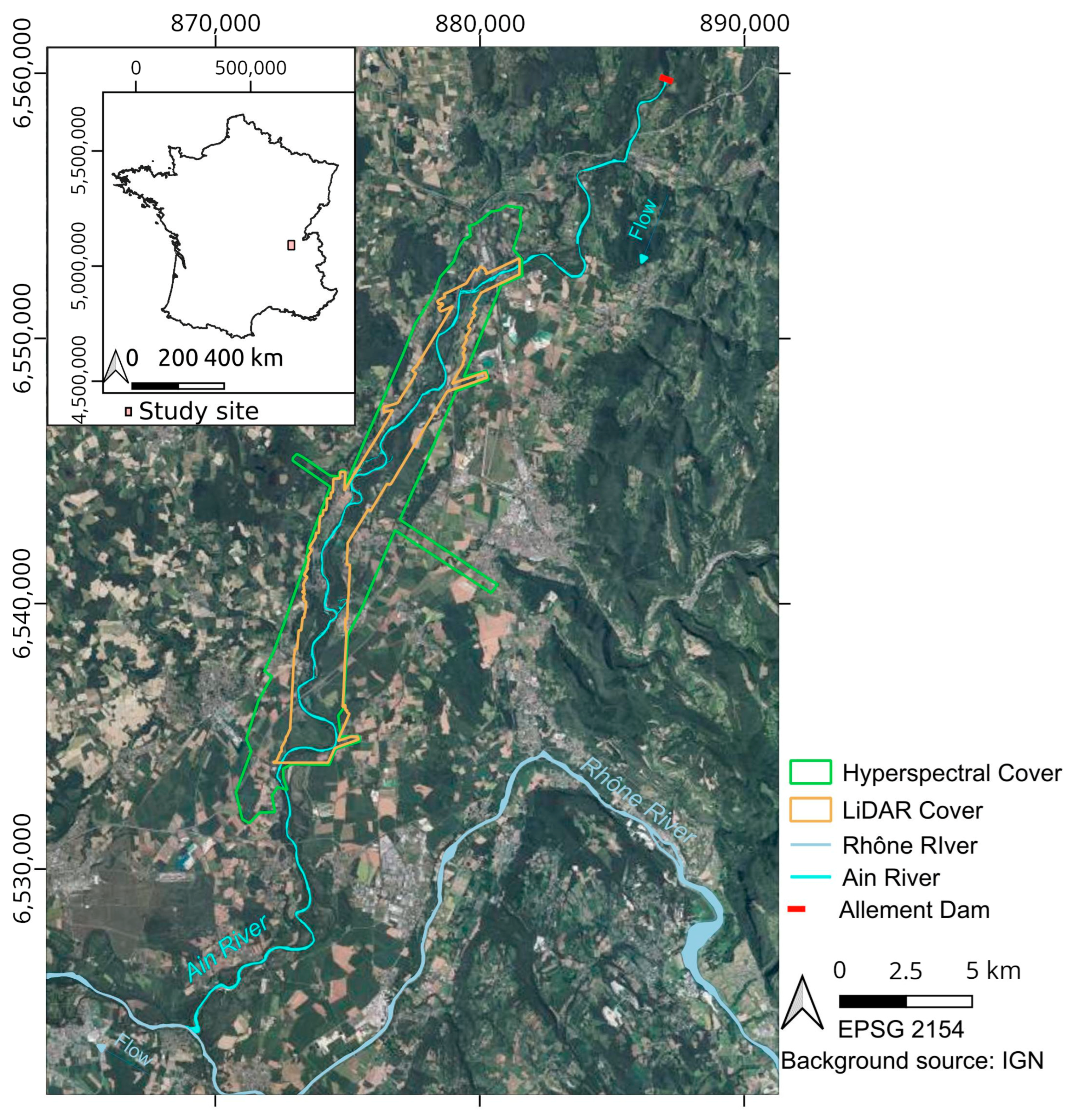
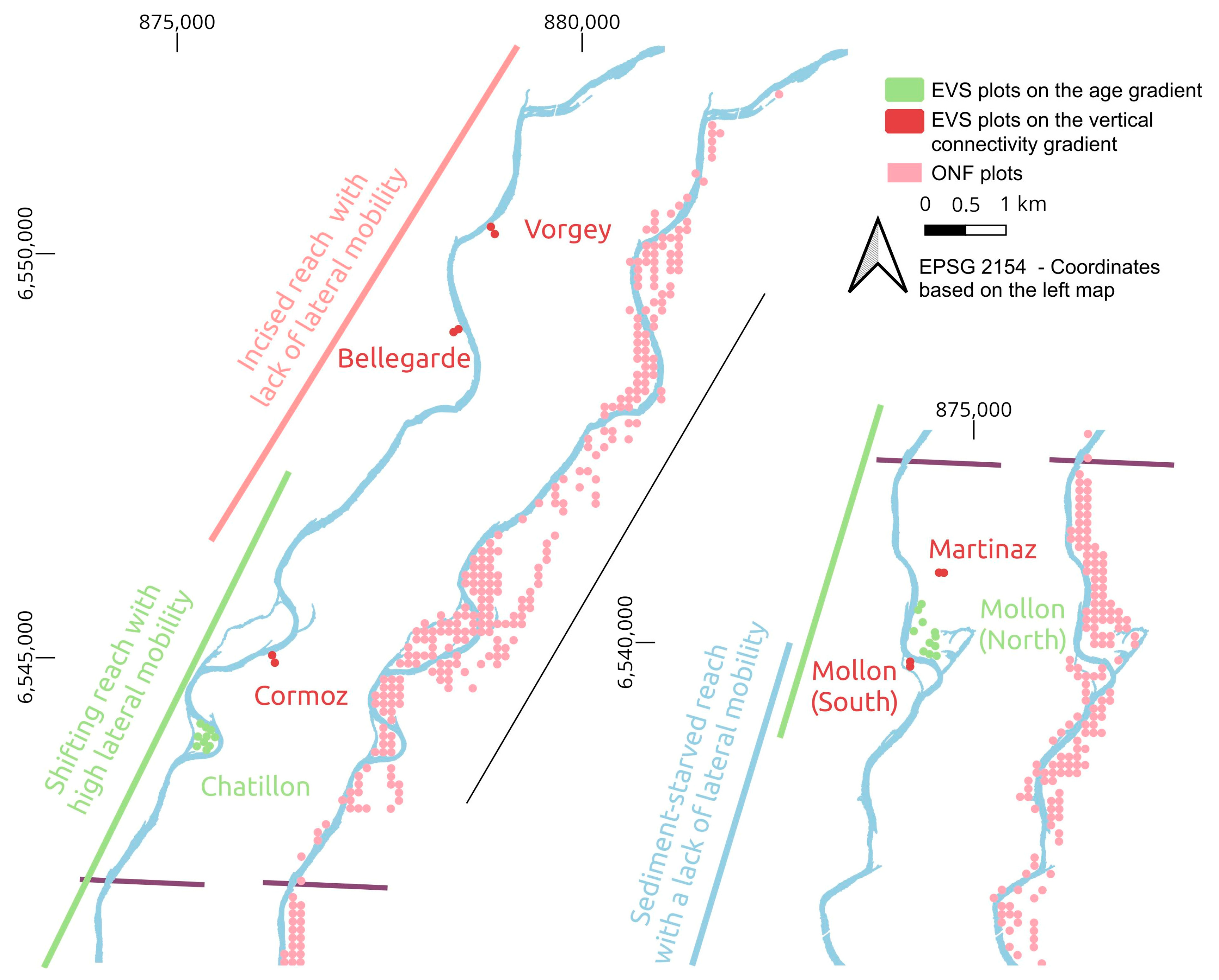
First, we expected that such data would show that some patches become higher, are less affected by overflow sedimentation, and progressively shift from pioneer species to post-pioneer hardwood species along the age gradient. Second, we expected that remote sensing information would be able to show that patches along the hydrological connectivity gradient (considering a similar age-group) become dryer and their vegetation structure becomes less homogeneous and sparser. In both cases, coupling hyperspectral and LiDAR data for the analysis should allow for quantitative estimation of the physical and temporal thresholds associated with important shifts.
We explored these two issues on the Ain River, France, where combined airborne and field data exist within a well-established geomorphic framework [61]. In our analysis, we first took a look at the topographic, structural, and spectral information for the selected forestry plots. Two sites were selected because they have good hydrological connectivity, while also featuring a mosaic of ages with plots ranging from three to forty years old (y.o.). Other sites were selected based on previous studies featuring mature riparian forest of a similar age, but on a gradient of hydrological connectivity due to channel changes (e.g., incised vs. stable or slightly aggrading channels).
We then expand this analysis over a dataset representing 400 ha of riparian forest for which forestry data is available, to see whether similar trends can be identified. Then, we use random forest classification to try to target different indicators of forest connectivity in a riparian landscape.
We can then create maps of the hydrological connectivity of the riparian forest of the Ain River and compare them with preexisting information on the variations in geomorphic characteristics inside the study reach [61].

2. Study Site

The study area is located on the Ain River, which is a large meandering gravel-bed river that is one of the main tributaries of the upper Rhône River, France (Figure 1). In the early 20th century, its fluvial pattern shifted from a braided one towards a sinuous single-thread pattern [62]. Changes in pastoral and silvicultural practices after the Second World War led to colonization of the river’s terrestrial margins [63] by a riparian forest whose main species are black poplar (Populus nigra) and European ash (Fraxinus excelsior).
The free meandering pattern of the Ain River leads to erosion of the older portions of the riparian forest and the creation of gravel bars that are colonized by willow species (Salix alba, Salix elaeagnos) that trap finer sediments and progressively aggrade, allowing colonization by poplars [64]. As the black poplars reach a height greater than that of the willows, other species appear in the understory, such as Norway maple (Acer platanoides), sycamore (Acer pseudoplatanus) and small-leaved lime (Tilia cordata) on dryer soils, while the pioneer willows die off (Figure 2). In older portions of the forest, Fraxinus excelsior overtakes Populus nigra as the most abundant species in the forest. In addition, invasive species, such as ash-leaved maple (Acer negundo) and Japanese knotweed (Fallopia japonica), tend to colonize the younger more-connected portions of the forest, to the detriment of the typical early pioneer species, such as willows.
During the 20th century, a chain of dams was built for hydroelectric purposes upstream of the study reach, with these including the Vouglans dam, which has a reservoir of 600 million cubic meters and induces downstream sediment starvation that propagates 500 m per year on average [61]. As a result, the incision of the riverbed progresses downstream, and only certain portions of the study reach are still sufficiently geomorphologically active to enable rejuvenation of the riparian forest through channel shifting and maintenance of a groundwater level close to the surface.
The impact of these anthropic drivers on the health of the forest has started to be assessed, mostly through long and costly traditional in-field vegetation surveys by the French National Forestry Office (ONF), conducted in 2006 and 2017 [65,66]. These surveys showed that the proportion of poplars and willows is decreasing, and that rejuvenation only occurs in the shifting reaches of the river, which are also associated with an increase in exotic species. A Landsat-based study [67] suggested that the impact of these anthropic drivers on forest health could be assessed through the use of remote sensing, but the spatial scale at which the study was conducted was too limited to assess anything other than a downward trend in the NDVI.
Therefore, the riparian forest of the lower Ain River basin can be considered a complex mosaic, where issues concerning species distributions, rejuvenation, and water stress intertwine as a result of the geomorphological changes that have taken place over the last century. Given the extensive datasets available, this carefully selected case study provides a unique opportunity to study the characterization of riparian forests.

3. Materials

3.1. Remote Sensing Information

The remote sensing data used in this study includes airborne hyperspectral imagery acquired in 2015, two airborne LiDAR surveys (in 2008 and 2015), and a series of aerial photographs that were acquired from eleven campaigns since the 1940s (Table 2).

3.1.1. Hyperspectral Imagery

On 29 September 2015, airborne hyperspectral imagery was acquired as part of a project funded by the European Facility of Airborne Research (EUFAR).
The remote sensing campaign led to the acquisition of twenty hyperspectral flight lines imaged with a Specim AISA Fenix hyperspectral camera sensor flown on a NERC-ARF (Natural Environment Research Council Airborne Research Facility) aircraft. This sensor consisted of two detectors that enabled the coverage of a spectral range between 380 nanometers and 2500 nanometers. The mean full width at half maximum across the 361 spectral bands was 3.98 nanometers. A mean flight altitude of 720 m resulted in each image having a ground resolution of 1 × 1 m.

3.1.2. LiDAR Data

The EUFAR dataset was complemented by a topo-bathymetric LiDAR acquisition made over the study reach in August 2015. This campaign was acquired at the request of Electricité de France (EDF) to study the bathymetry of the river channel [68]. An Optech Titan sensor was flown on an aircraft 329 m above the ground, resulting in around ten billion data points. The final point density was 18.6 points/m2 for each laser, and the vertical accuracy was around 10 cm.
A second and older LiDAR dataset was also used in this study. This dataset was acquired on the 6 and 8 March 2008. However, only a post-processed point cloud without the vegetative cover was available; therefore, it was only used in conjunction with the 2015 topo-bathymetric LiDAR data to extract information related to sedimentation or erosion under the canopy cover between the two dates.

3.1.3. Series of Aerial Photos Since the 1940s

Historical aerial photographs produced by the Institut National de l’Information Géographique et Forestière (IGN) were used to assess the age of riparian vegetation by photo interpretation. These data were collected over 11 campaigns from 1945 to 2012 and were available for the following years: 1945, 1954, 1963, 1971, 1980, 1991, 1996, 2000, 2005, 2009, and 2012. The gap between acquisitions has become shorter in more recent years, and color images have been acquired since the 2000 campaign. The ground resolution of the images varied between 100 and 50 cm per pixel.

3.2. Field Calibration Data

3.2.1. Vegetation Survey during the Airborne Campaign in 2015

Following the 2015 acquisition, fieldwork was conducted in September and October by the EVS laboratory staff to survey the riparian forest in thirty plots with a 10 m radius (Figure 3).
The central position of each plot was acquired with a GeoExplorer 6000 handheld global positioning system. Within a ten-meter radius, each individual tree with a diameter above 30 cm was referenced to a database, and its height was recorded (Table 3). In addition, all individual trees with a diameter above 7.5 cm within a smaller five-meter radius were also referenced to the database. The tree species were assessed according to leaf morphology. Soil-related information, such as organic matter and sediment size, was also assessed.
The locations of the plots were decided, so that the surveys included: (1) two series of plots along an age gradient in shifting reaches of the river, and (2) one series of mature forest plots of the same age along a gradient of vertical connectivity.
The two series of plots sampled along the age gradient (Chatillon and Mollon North) benefited from the lateral mobility of the river. The fluvial dynamics of the reach allow for the creation of new gravel bars, and their colonization by new pioneer vegetation. This mobility helps maintain forest rejuvenation and leads to patches differing in age (from 4 to 40 years for the plots sampled along this gradient) and developmental stage within the same geographic area.
In comparison, the vertical connectivity gradient includes forest plots that are of the same age (70–80 years) but are spread out across differing levels of lateral mobility and channel incision. These plots were chosen on the basis of previous studies conducted by Dufour [63] that highlighted differences in the growth of European ash, depending on the elevation of forest plots, relative to the water level of the river, which affects the distance to groundwater and the frequency of flooding. We consider them to be mature forest plots in the case of the Ain River riparian forest because they belong to the later successional stages identified by the ONF and to some of the oldest sectors of the riparian forest.
Both the Mollon (South) and Martinaz plots are located in the river reach with the highest lateral mobility and feature a low vertical elevation, although the high lateral mobility has resulted in a shift in the main channel in recent years, which explains why the Martinaz plots are laterally distant from the river channel.
Of the remaining sites, the Bellegarde site and the Vorgey site are located in the incised sector of the river, whereas the Cormoz site is near the frontier between these two geomorphic sectors and is situated on an elevated outer bank of the river channel. All three of these sites feature a higher elevation, relative to the river level than the Mollon (south) and Martinaz sites and, therefore, lower degrees of hydrological connectivity.

3.2.2. The Extensive Vegetation Surveys Performed in 2008 and 2017 by ONF

The vegetation surveys (for which remote sensing information was acquired) conducted by the ONF at the request of the local stakeholders in 2008 and 2017 covered c. 400 plots in the study reach, one per hectare of forest (see Figure 3 and Table 2).
For each vegetation plot, the basal area of each species and the total basal area were measured using a relascope. This basal area measurement corresponds to the superficy (assumed to be circular) of a cross-section of the tree at 1.3 m from the ground. Additional information, such as grass cover, was collected within a five-meter radius to assess the ecological diversity of the plot. Information on the presence or absence of key invasive species, such as Fallopia japonica and Acer negundo, was added to the survey database. Species were determined using an identification key focusing on twigs. The soil depth and humidity were also assessed for each plot.
The age indications in this dataset came from post-hoc assessments by the ONF team and relied on identifying the year of colonization by looking at the series of historical aerial photographs, described in Section 3.1.3.
The field operators who performed these surveys were trained forestry professionals and were different from the team of EVS researchers that conducted the survey described in Section 3.2.1.

4. Methods

The methodology used in this paper is divided into four different steps, as shown in Figure 4. First, forest indicators were extracted from the LiDAR and hyperspectral data, providing information about the forest structure, spectral reflectance, and the topography of the corresponding forest plot. Then, this expanded dataset was coupled with the vegetation field surveys, in order to explore the characteristics of the riparian forest along an age gradient from early pioneer individual trees that have not yet reached maturity to later successional stages dominated by 50+ year poplars and post-pioneer species. By simultaneously exploring these characteristics along differing geomorphic reaches, we then studied how forest plots of a given age are impacted by reach-scale geomorphic features, such as channel incision and sediment starvation.
Finally, random forest classifiers—using remotely sensed indicators generated from LiDAR and hyperspectral data as predictors—were constructed to discriminate between different hydrological connectivity levels according to key target species (for wet and dry environments), identify the transition from pioneer poplar forest towards post-pioneer hardwood forest, and identify growing and mature forest patches. The resulting classifications were used to map the key characteristics of the riparian forest along the 20-km reach of the lower Ain River basin and provide a view of the resulting spatial trends at the reach scale.

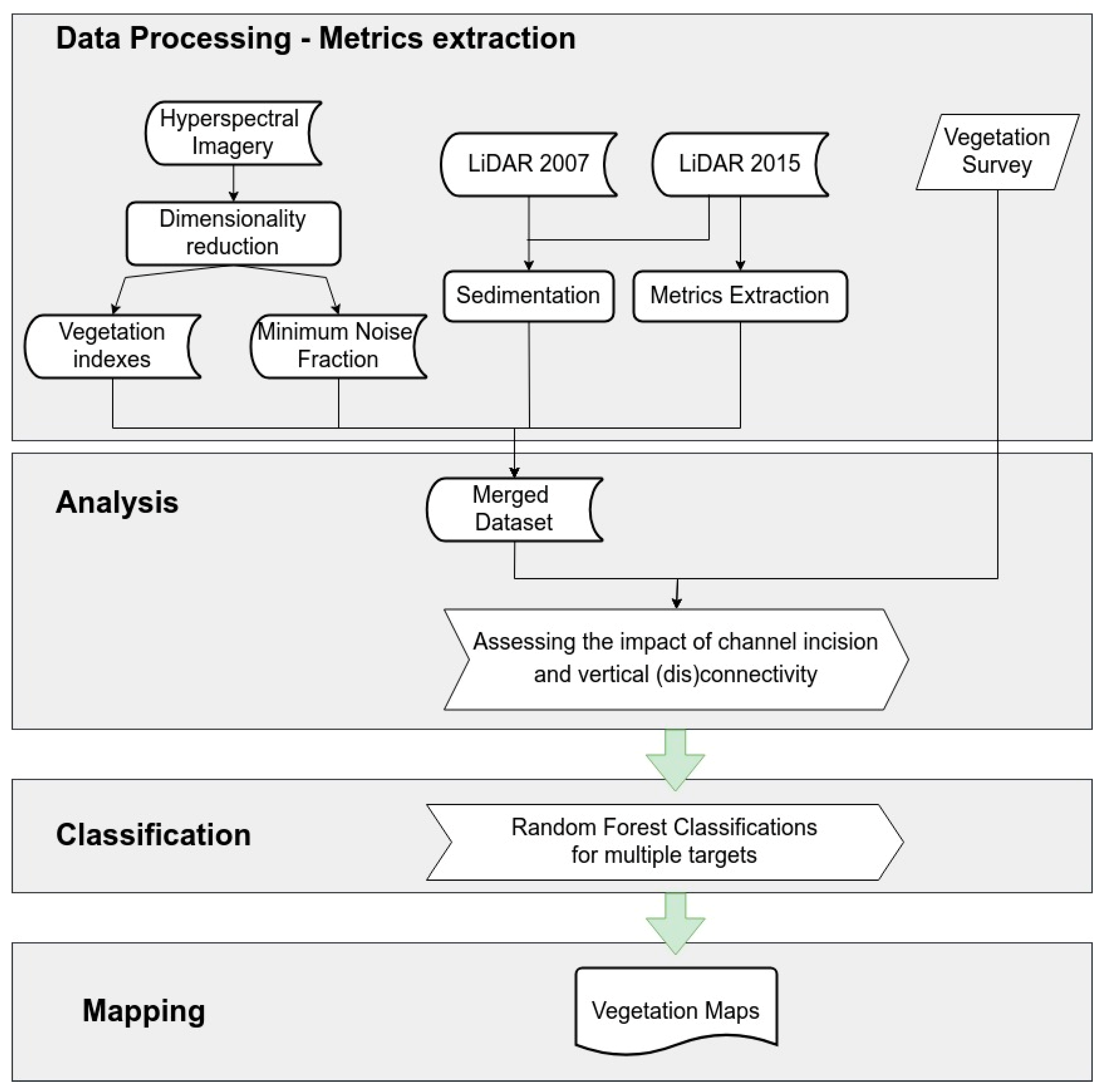
4.1. Data Processing: Extracting Forest Indicators from Hyperspectral and LiDAR Data

Both the hyperspectral and LiDAR datasets were processed to facilitate the extraction of metrics at the plot level. The complete list of metrics can be found in Appendix A, and for each metric, the mean, minimum, maximum, variance, and standard deviation were extracted for each plot in the EVS and ONF dataset.
The LiDAR data from 2015 were initially processed using the lidR library [69] to extract a digital elevation model (DEM), digital height model (DHM), and structural vegetation metrics. The Fluvial Corridor Toolbox [70] was then used to detrend the DEM, relative to the water level under low-flow conditions (Q = 16 m3/s), to provide the relative elevation of each plot, with respect to the water level.
Further processing included using SAGA GIS [71] to extract a wide range of plot-level topographic indexes found to be relevant for riparian grassland classification in a previous study [56].
The LiDAR data from 2008 were also processed using the lidR library to extract a DEM. Only this information was extracted from the data because only ground points were present in the available post-processed point cloud. This digital elevation model was then subtracted from the 2015 model to assess sedimentation processes, according to the difference in plot elevation between the two dates.
The accuracy of this process was assessed by choosing 12 ground control points along the study reach in areas that we assumed to have a stable elevation (such as roads and fields) and looking at the difference in vertical elevation between the two LiDAR datasets for these control points. This resulted in a mean error of 9.6 cm and a median error of 9.5 cm.
Since the spatial coverage of the second LiDAR dataset was also limited, it was not used as a predictor for the random forest classification in step 3 of the methodology, but only to help characterize the vegetation plots in step 2 of the analysis.
For the hyperspectral imagery, a minimum noise fraction was produced, in order to denoise the initial image into meaningful bands holding the majority of the spectral information. The minimum noise fraction was calculated for only the vegetated area of the hyperspectral image by applying a vegetation mask based on the LiDAR-derived canopy height model. In addition, a set of hyperspectral vegetation indexes were calculated, with these targeting key vegetation features, such as pigmentation, greenness, and canopy water content (listed in Appendix A).

4.2. Data Analysis: Studying the Riparian Forest by Assessing the Impact of Channel Incision and Vertical (Dis) Connection to the River System

The data processing phase was then followed by a more classical analysis of forest characteristics, in which they were plotted against the age of the forest and grouped by geomorphic reach (incised, shifting, and sediment-starved). This allowed for visualization of the impact of age on the riparian forest by looking at how individual characteristics evolved through time, and also allowed for trends in forest plots between geomorphic reaches of the same age to be distinguished.
Topographic changes were explored first to better understand the changes in site conditions along both the age and connectivity gradients. Overbank sedimentations and the LiDAR-derived elevation of the forest plot, relative to the water level of the river during low-flow conditions, were used as proxies for forest connectivity (depth to groundwater and flooding frequency), while field survey data provided information about soil development.
Changes in species compositions were then explored to better understand the response of the communities to the changes in site conditions occurring along the two gradients.
Finally, the resulting estimates of changes in the structure of the riparian forest and the reflectance of its canopy were explored by focusing on forest height, canopy greenness, and canopy water content. Variations in forest structures were tested against variations in biochemical characteristics to better understand which of the changes could be driven by stress responses.

4.3. Random Forest Classifications of Forest Connectivity and Resulting Maps

Following the analysis of the forest characteristics, random forest classifiers were constructed for the four different classification targets of age group, forest type, presence of Fallopia japonica, and presence of Tilia cordata (Table 4). All the indexes listed in Appendix A were used as inputs to the classifiers, and a randomly sampled dataset of 50 plots was used for each class.
The classification targeting age groups attempted to distinguish between the growing forest and mature forest patches. Growing forest patches are likely to be located in areas where lateral mobility occurs and leads to forest rejuvenation, whereas mature patches are likely to be located on either well-connected areas of the river that have not yet been eroded or along reaches impacted by sediment starvation. For practical purposes, we distinguished between the “growing” and “mature” types of forest patches by referring to the age at which plot composition shifts towards post-pioneer and vegetation height (therefore, the height of poplar trees in the plot) reaches its maximum. This results in the “growing” class targeting the parts of the riparian forest that are of interest for the local stakeholders, due to having higher patrimonial value.
The forest type classification attempted to distinguish the dominant species at the canopy level. The poplar forest is likely to be located in growing forest patches and well-connected mature forest patches, whereas the post-pioneer forest is the development stage where the poplar population is replaced by the European ash on presumably older and less-connected forest plots.
The last two classifications target the presence or absence of key indicator species that prefer specific soil conditions. In addition, Fallopia japonica is presumably not present in the forest plots at the canopy level. These two classifications provide information about site conditions.
To better understand the classifiers, the best-predictive variables were identified for each of them, and their results were compared with a pre-existing plot classification performed by the ONF and based on field characteristics, such as species composition and stem diameter.
In addition, the classifications were also attempted using only LiDAR data or only hyperspectral data to determine whether both are required for such applications.
Finally, the results from the classifiers were mapped and checked against the three geomorphic reaches to better understand the spatial trends of connectivity of the riparian forest of the Ain River at the reach-scale.

5. Results

5.1. Exploring Forest Characteristics and Their Evolution along the Age Gradient at Varying Degrees of Hydrological Connectivity

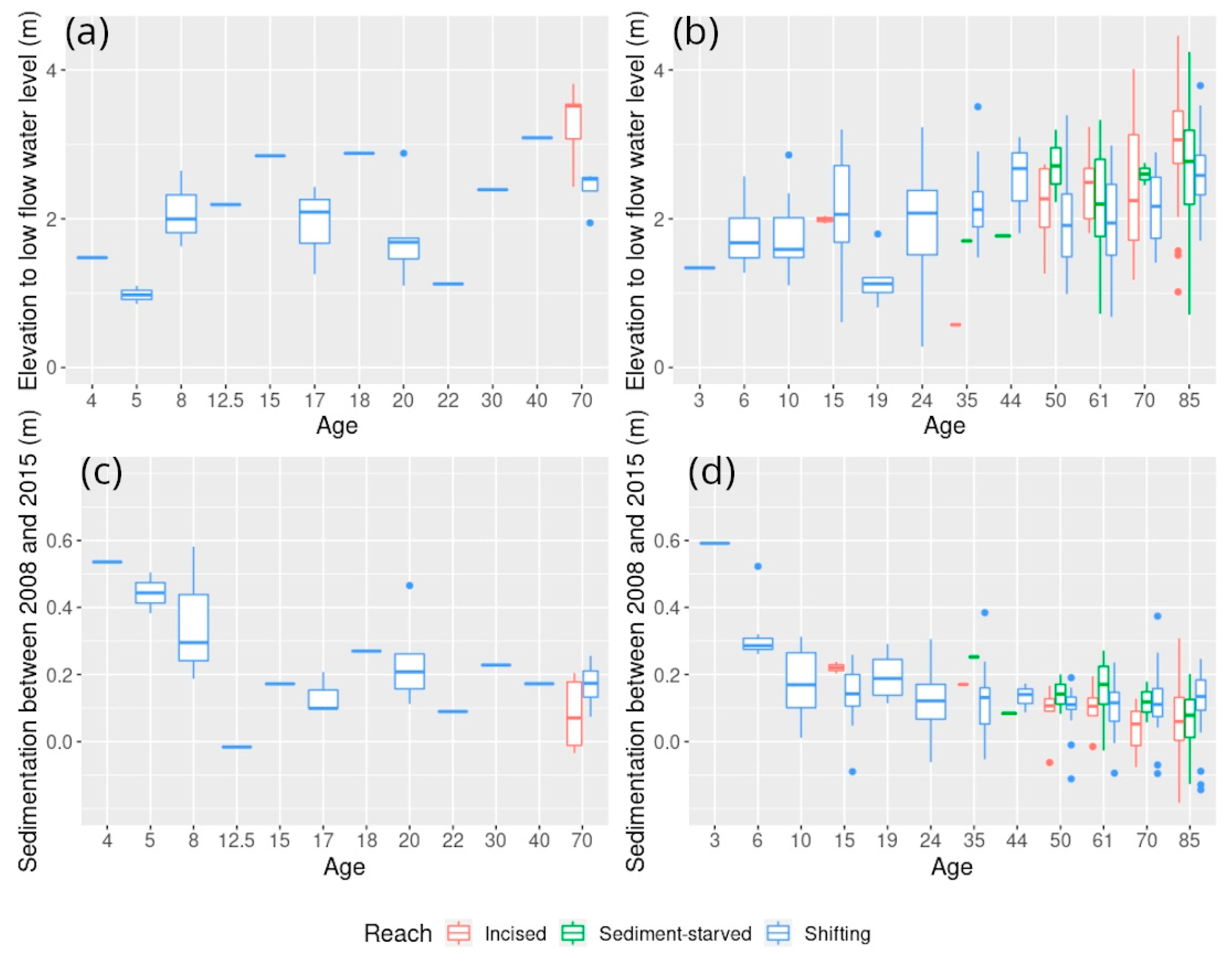
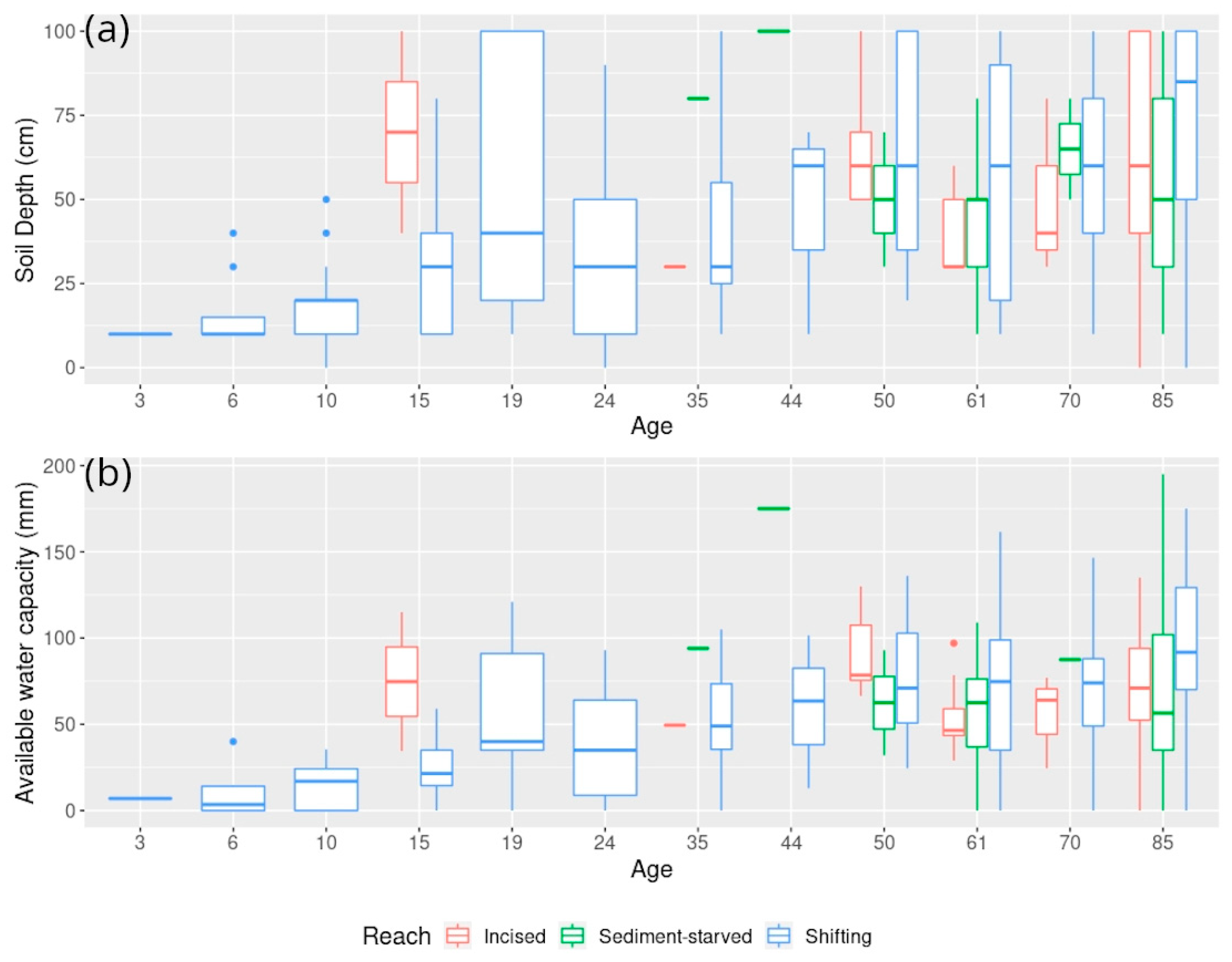
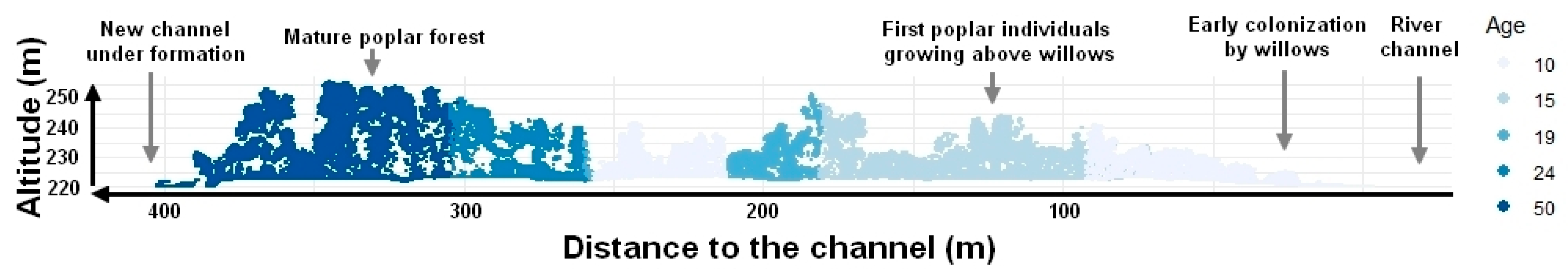
5.1.1. Characterization of Hydrological and Sedimentological Changes

First, two physical indicators of hydrological connectivity derived from the remote sensing data were explored for both forestry surveys: (1) the elevation of vegetation plots relative to the water level of the river (measured under low-flow conditions), and (2) overbank sedimentation under the canopy cover between 2008 and 2015 (Figure 5).
Both overbank sedimentation and the elevation of plots, relative to the water level of the river, provide information about flooding frequency, and therefore, hydrological connectivity, whereas plot elevation also provides information about the distance of the vegetation plot to groundwater resources. Hence, lower overbank sedimentation and higher plot elevation are representative of dryer physical conditions in the corresponding vegetation plots.
The elevation relative to the low-flow water level was lowest for the youngest forest plots of the EVS dataset, which are located on recently-formed gravel bars (Figure 5a). After these, the elevation rose quickly because most forest plots above 8 years old were located two meters above the low-flow water level. Because of the free meandering mechanics of the Ain River within this reach, some of the older plots (17 y.o., 20 y.o., and 22 y.o.) were located near to topographic depressions, such as paleo-channels and cut-off reaches, and featured a lower elevation (<2 m). This suggests that local fluvial dynamics can induce variability in plot elevation within a given reach and for a given age; for example, low elevation due to the presence of paleo-channels that are closer to the water table.
A similar trend can be observed in overbank sedimentation, which relies on frequent flooding and its associated with sediment deposition to drive an increase in plot elevation. The sedimentation rate is initially high for the youngest EVS plots (>20 cm), then drops sharply after ten years, reaching values hovering between 10 and 20 cm (Figure 5c).
Overall, the two indicators combined show trends of increasing elevation and decreasing sedimentation with age, reaching a plateau during the first ten years after plot colonization. This is also the case for the ONF dataset, which provides a more extensive view of the riparian forest of the Ain River, but one in which plots are less homogeneous in age.
Indeed, in the ONF plots, the elevation relative to low-flow water level (Figure 5b) was, on average, lower than two meters for plots up to 10 years old and for the few 19-year-old plots, but was two meters or higher when riparian vegetation was older, reaching values above four meters for some of the oldest plots. The mean overbank sedimentation of plots younger than ten years was above 20 cm, reaching as high as 60 cm on one plot, but this value dropped sharply afterwards, with sedimentation reaching values closer to 10 cm on average (which was also the mean error for the vertical difference between the two LiDAR studies in locations with stable altitude) (Figure 5d).
However, age is not the only driver of change evident on Figure 5, as there are differences between the river reaches with lower lateral mobility (the incised reach and the sediment-starved one, where lateral mobility is constrained by morainic deposits) and the shifting reach of the river where lateral mobility is high. Plots of the same age located in the incised or sediment-starved reaches, as opposed to the shifting reach of the river, feature a higher elevation relative to the water level of the river (averages for different ages varying between 50 and 100 cm) and lower sedimentation (averages for different ages varying by up to 10 cm).
Two field measurements focusing on the soil at the center of each of the forest plots were explored for the ONF dataset: (1) soil depth up to one meter measured by an auger (Figure 6a) and (2) the available water capacity of the soil (Figure 6b). Both measurements are important for the development of riparian vegetation because they affect root growth and the potential abundance of water resources in the upper layer of the soil.
Both soil depth and available water capacity increased with age in the shifting reach, with really low values in the early phase of riparian colonization (soil depth < 25 cm and available water capacity < 25 mm for plots up to 10 years old) when pioneer species help to trap finer sediments on the gravel bar. The values reached plateaus at around 60 cm for soil depth and 75 mm for available water capacity at ages ranging from 50 to 70 years, although plots older than 70 years featured higher average values for both indicators. In addition, the soil depth was probably underestimated because of multiple vegetation plots reaching the maximum depth that could be measured with the hand auger.
Similar to the two previous indicators of hydrological connectivity (elevation relative to low flow water level and sedimentation between 2008 and 2015), the values of soil depth and available water capacity for plots of a given age differ according to which of the hydrogeomorphic reaches of the river they are located in. Both the incised reach of the river and the sediment-starved reach downstream of the shifting reach feature lower soil depth and available water capacity for their age, in comparison with plots located in the reach with high lateral mobility.
However, plots less than 50 years in age do not appear to show the same trend. This is partly due to their low number overall (one observation for ages 35 and 44 and two observations for age 15). These plots are located really close to older and mature forest plots, which may introduce variability, depending on the quality of the geo-referencing and the location of the measurement within the plot.
To summarize, all four indicators show changes along two different gradients: an age gradient that accompanies vegetation growth and a hydrological connectivity gradient that highlights differences between vegetation plots of the same age that are not located in the same geomorphic reach of the river.
The shifting reach, where erosive processes are still occurring, appears to be the one with highest hydrological connectivity, since the rejuvenation of riparian vegetation still occurs in the reach after 1965, contrary to the other two reaches. On average, even older forest plots feature lower elevation (relative to the water level of the river), higher sedimentation, and deeper soil with higher available water capacity. Both of the other reaches seem to be degraded, compared with this reference state, with the incised reach upstream of the study site tending to appear as though it has slightly worse hydrological connectivity than the sediment-starved reach downstream of the shifting portion of the river.

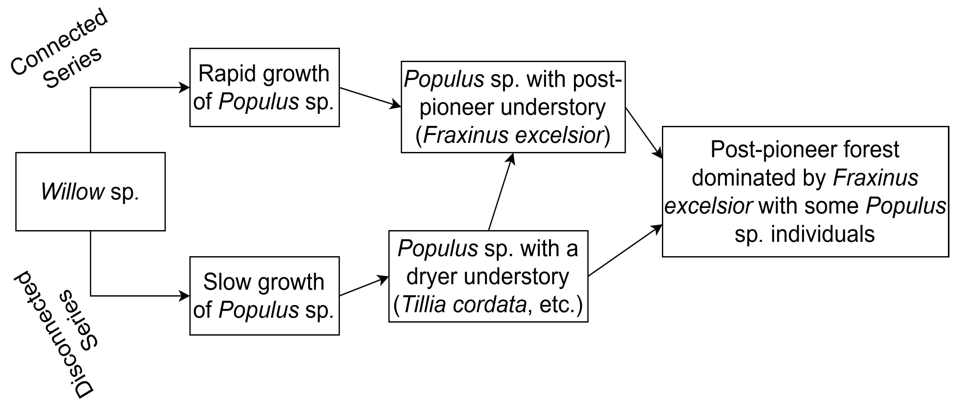
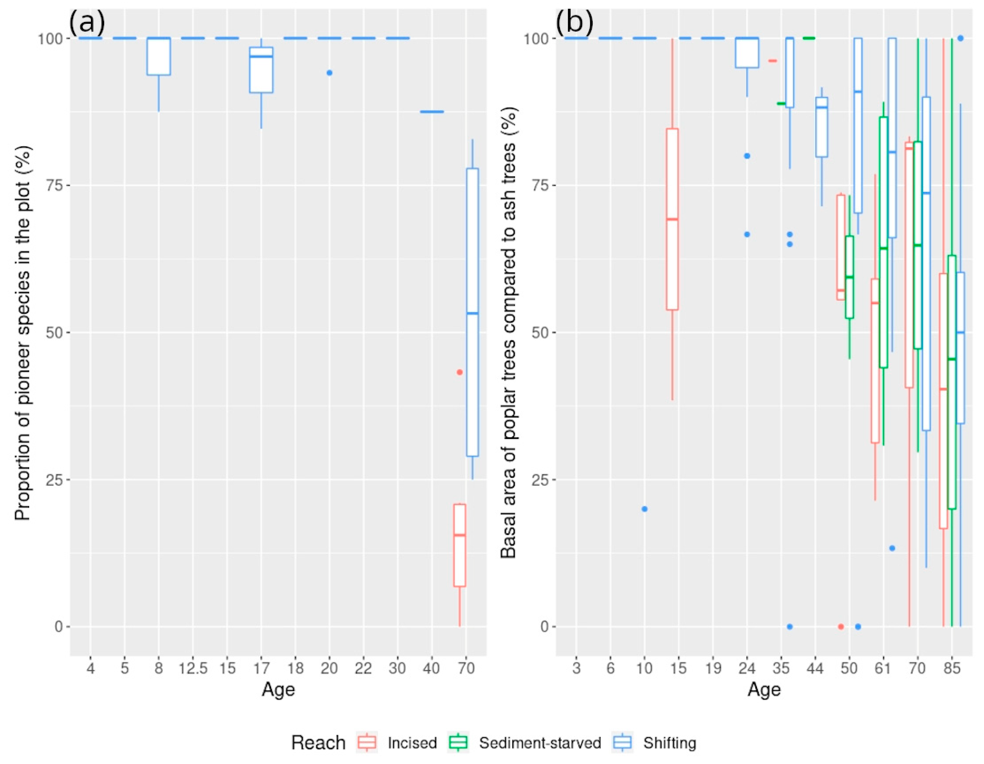
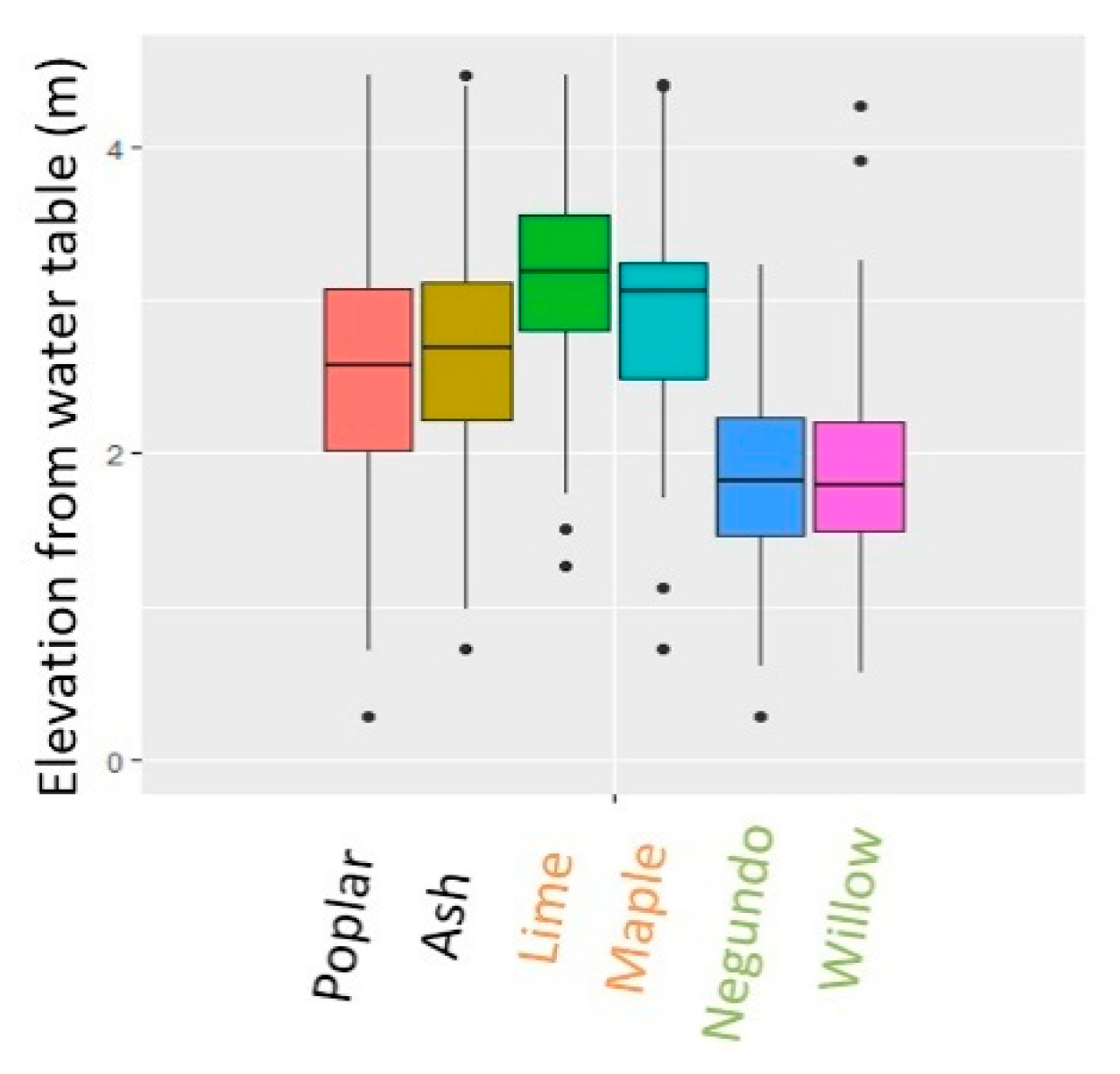
5.1.2. Associated Changes in Species Composition According to Field Surveys

The plots sampled by the EVS survey mainly comprised pioneer riparian species such as Salix sp. and Populus nigra, whose colonizing ability relies on frequent flooding (Figure 7a). Post-pioneer species, such as Fraxinus excelsior, only become more abundant in the older plots that were sampled on the vertical connectivity gradient (70 y.o.) across both the shifting and incised reaches of the river. This shift towards more post-pioneer compositions was more advanced in the plots sampled in the incised reach of the river, with only 20% of pioneer species remaining in a given plot, while 50% remained in the plots located in the shifting reach.
The same trend can be observed for the extensive ONF dataset, which shows the colonization of forest plots by Fraxinus excelsior after 30 years (Figure 7b). Once again, this colonization is more advanced for plots in either the incised or sediment-starved reaches of the river, compared with plots located in the shifting reach. This suggests that the hydrological disconnection caused by the incision of the riverbed creates an environment that is more favorable to Fraxinus excelsior than to the typical pioneer species of the Ain River.
In the case of the survey conducted by EVS, this variation in hydrological connectivity results in the presence of an abundance of species that prefer to colonize dryer soils (Table 5). On the Vorgey and Cormoz sites, Tilia cordata can account for half of the individual trees in a given plot, whereas only one or two individuals have been recorded (when present) on plots with better connectivity, such as the Mollon and Martinaz plots. Those plots with lower connectivity are also favored by shrub species, such as Corylus avellana and Crataegus monogyna.
In addition, the few plots that have not been colonized by Fraxinus excelsior are the ones with the highest amount of Tilia individuals and shrub species, which suggests that, in some locations, the soil is too dry to be favorable to the growth of Fraxinus. However, the vegetation in the Bellegarde site does not contain Tilia individuals and shrub species, despite being located in the incised reach of the river. Instead, the vegetation in these two plots consists of mostly post-pioneer species, with species associations typically found in continental forests, such as Acer campestre, Acer pseudoplatanus, Acer platanoides, and Quercus pedunculata.
Similarly, on older vegetation plots (>50 y.o.) from the ONF survey, those species with a preference for dryer soils (Tilia cordata) or a more mature post-pioneer environment (Acer sp. other than negundo) were present on forest plots with a high elevation, relative to the water level at low flow (Figure 8). On the contrary, plots where a few individuals of Salix sp. or the invasive Acer negundo remain had a lower relative elevation, although they may also be located in plots of less homogeneous age. In this case, the empirical cut-off in relative elevation between these two different compositions appears to be around 2.5 m, which once again highlights the role of vertical (dis)connectivity in the composition of riparian forests.
To summarize, the composition of the riparian forest shifts with age and depends on the vertical connectivity of a given forest plot. Post-pioneer species, such as Fraxinus excelsior, colonize already established forest plots dominated by traditional or invasive pioneer species (Populus nigra, Salix sp., and Acer negundo). This shift towards a more post-pioneer environment is more pronounced for forest plots located in the incised or sediment-starved reaches of the riparian forest, which are also those plots with lower hydrological connectivity (lower flooding frequency, high depth to groundwater, and lower soil water capacity). This shift is also associated with the development of shrub species and the growth of Tilia cordata, which can become dominant in the driest forest plots.

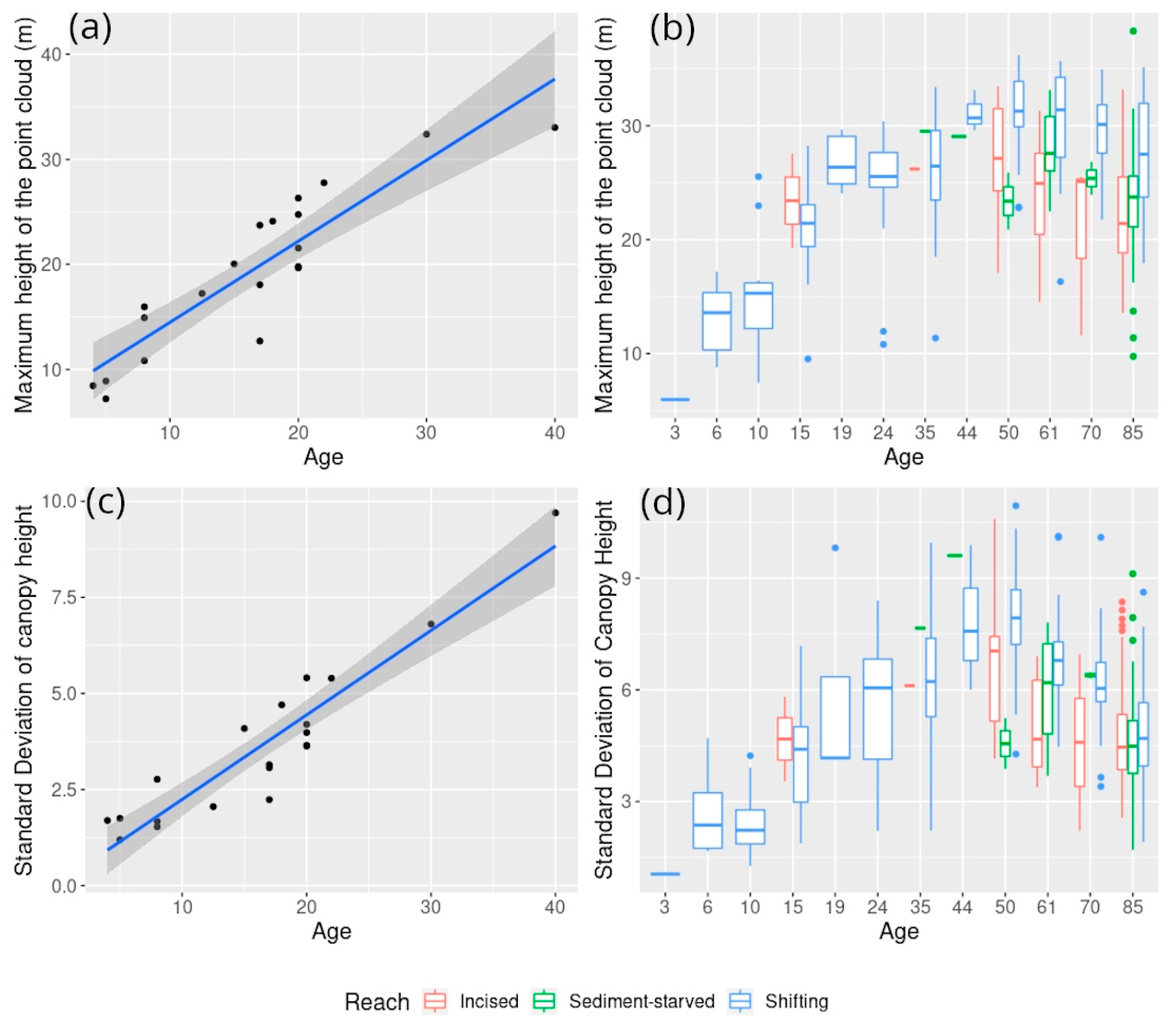
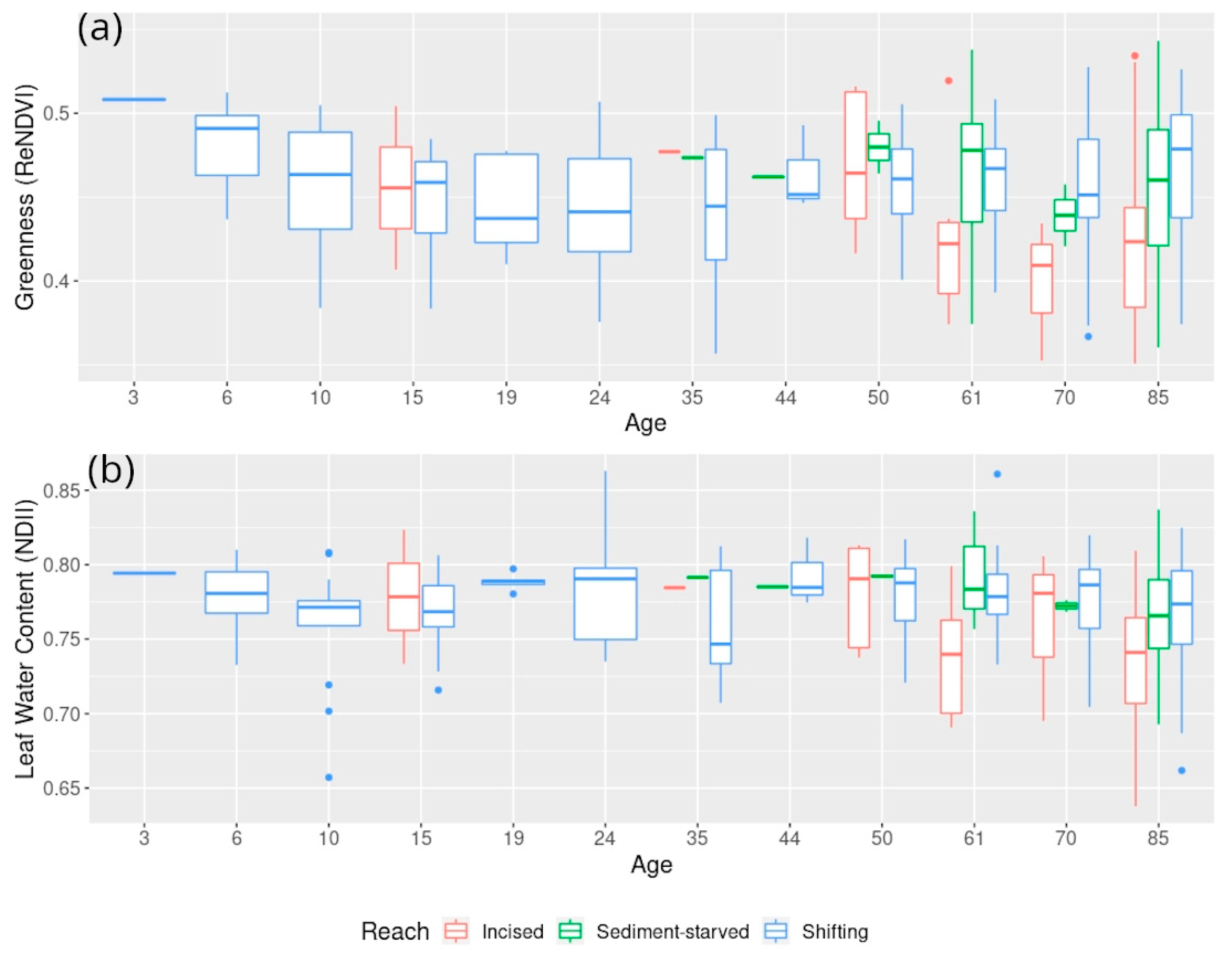
5.1.3. Associated Changes in Forest Structure and Reflectance

As illustrated by a transect of the LiDAR data over the Chatillon site, the structure of the riparian forest changes with age (Figure 9). The early developmental stages of the riparian forest are illustrated by such a transect: the early stages of the floodplain are colonized by willows, and then the poplar trees grow higher than the willow trees, which progressively leads to the development of a more mature pioneer forest, in which an understory can develop.
This growth can be seen at the plot level through structural indexes such as the height of the vegetation in the plot or the standard deviation of canopy height (Figure 10). In the case of the forest plots from the EVS survey sampled along the age gradient, the linear relationship between the age of the plot and the height of the canopy (20 observations in Figure 10a) is strong, with an r2 of 0.82 and a residual standard error of about four years. The standard deviation of canopy height (20 observations in Figure 10c) is also linearly correlated with plot age, with an r2 of 0.87, and a residual standard error of about three years. In both cases, the error from the regression is close to the gap in years between the aerial photographs that were used to determine the age of each plot (one campaign every three to five years for the most recent ones).
The growth of the riparian forest with age is also visible in the plots from the ONF survey, even though the age of each individual plot is less homogeneous. Both the height of the canopy in the plots (Figure 10b) and its standard deviation (Figure 10d) increases with age, until it reaches a plateau in the case of height or decreases in the case of standard deviation at around 40 years. Once again, age is not the only explanatory factor, as forest plots on the incised or sediment-starved reaches tend to have a lower maximum canopy height, compared with plots of the same age in the shifting reach, as well as a lower standard deviation of canopy height.
These changes in the maxima and standard deviation of canopy height also illustrate the successional stages of the riparian forest, with the poplar trees growing above a more uniform shrub-land of willows, therefore giving an increase in canopy height and its standard deviation. When the poplar trees reach maturity, the height of the canopy tends to no longer increase, and as the forest develops, the difference in height between trees in the plot is reduced. However, the changes in the maxima and standard deviation of the canopy height also suggests an impact of the vertical connectivity gradient of the riparian forest, with plots with less access to groundwater and frequent flooding (in the incised and sediment-starved reaches) featuring lower maxima of tree elevation, either due to poplars not growing as high or due to the transition towards smaller post-pioneer species.
This relationship between access to groundwater and tree structure can be assessed using hyperspectral indexes of greenness and canopy water content, such as the ReNDVI or the NDII (Table 6). Although the correlation between height and spectral indexes traditionally used to detect forest or crop stress is low for growing forest plots (≈100 observations), it increases to around 0.5, when only mature forest plots are considered (>50 y.o., ≈300 observations).
This suggests that lower accessibility to the water resource and the resulting stress on individuals or communities is one of the driving factors behind the structural variability of the riparian forest, and that it can be detected using hyperspectral indexes. Indeed, both greenness and canopy water content tended to be lower in forest plots located in the incised or sediment-starved reaches than in the plots located in the shifting reach of the Ain River (Figure 11).

5.2. Can We Predict and Map the Shift in Forest Composition, Structure, and Reflectance That Results from Vertical (Dis)connection of the Riparian Forest Due to Channel Incision?

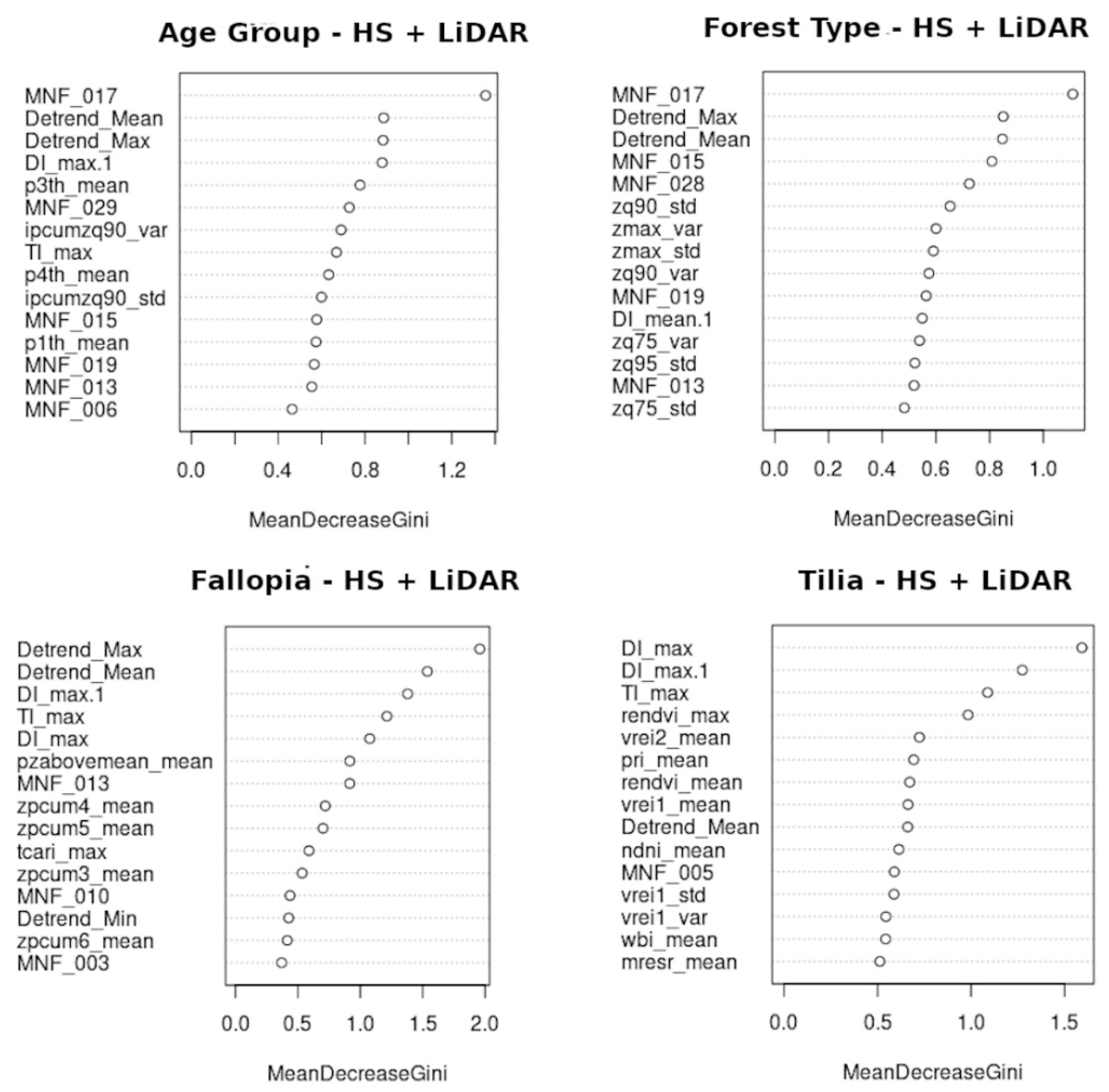
5.2.1. Random Forest Classifications

Random forest classifiers were trained on four distinct binary classification targets for the ONF plots to explore how LiDAR and hyperspectral data are able to predict key characteristics of the riparian forest (Table 7).
The best accuracy for the prediction of forest type was reached in the discrimination between the well-connected poplar forest plots (>75% black poplar trees) and post-pioneer hardwood forest (>75% European ash trees), with a class error between 12% and 14% when using both data types. The accuracy was also high when attempting the classification using only LiDAR (class error between 16% and 18%) or hyperspectral (class error between 18% and 20%) data.
Class errors lower than 20% were reached for the other classification targets when coupling hyperspectral and LiDAR data, resulting in an overall accuracy higher than 80%. This was also the case for predicting plots where the invasive Fallopia japonica or Tilia cordata were present or absent, even though these species are not necessarily dominant or present at the canopy level in the plots in the case of Fallopia japonica. Predicting species that do not present at the canopy level, coupled with the ability to predict degrees of plot elevation (and therefore distance to the water resource) using spectral and structural characteristics, suggests that the classifiers do not necessarily distinguish between specific species, but rather between the degrees of forest connectivity that were observed in the analysis of forest characteristics.
Overall, the class errors were similar once the classifiers were applied to all of the forest plots, instead of the 50 plots–50 plots training samples (Table 8), which suggests that the classifier did not overfit the training data. While the mean error between the two classes dropped slightly for all classification targets, the highest class error was achieved for predicting the presence of Tilia cordata. In this case, the classifier predicted the presence of Tilia cordata in almost a quarter of the forest plots in which the species is absent.
The best-predictive variables in the random forest classifiers were bands from the minimum noise fraction and spectral indexes targeting greenness (ReNDVI, VREI1), or canopy water content (NDNI, WBI) in the case of the hyperspectral data (Figure 12). For the LiDAR data, structural information, such as the variance of the standard deviation of the canopy height (zmax, zq90), and topographic indexes, such as the elevation above the base-flow water level (detrend) and direct insolation (DI), were the best predictors.
However, the mean decrease in gini (feature importance) was relatively low (<2%) for all of the classifications because a lot of the individual variables could be replaced by other correlated variables that achieved similar results.
Comparing the results of the classifications against the forest types determined by traditional forestry techniques by the ONF allows for a more precise look at the results of the classifiers and shows differences between classification targets (Table 9).
The early pioneer forest is defined as the first stage of forest growth and development by the ONF and is easily discriminated across all four classification targets: it corresponds to a poplar forest that is still young and is well-connected to the river channel, therefore being a favorable environment for the growth of the invasive Japanese knotweed.
Both the rapid-growth series and slow-growth series feature riparian forest plots that have not yet reached the most mature stage of growth (developed understory and large tree diameter) of the poplar forest on the Ain River, according to the ONF. The key difference between the two series is that the slow growth one is supposed to grow on elevated riverbanks that are less frequently flooded.
Half of the plots in the series were categorized as mature forest plots by the age group classifier, which suggests they had reached a forest structure similar to the one seen in most forest plots above 50 y.o, an age that the forest plots of both ONF types can reach because the limiting factor for the next stage is tree diameter.
In addition, plots from the slow-growth series, which should be less connected to the river system, are more often predicted as favorable to the development of Tilia cordata, whereas plots from the rapid growth series are more often classified as favorable to the development of Fallopia japonica, which fits with the concept that the main difference between these two forest types is their degree of hydrological connectivity.
Finally, when reaching the most mature stages of the poplar forest, where it transitions towards post-pioneer hardwood forest, the majority of forest plots are predicted as mature and are not favorable to the development of Fallopia japonica. However, less than half of them are predicted as being favorable for Tilia cordata, and half of the plots that the ONF surveyed as representing the final stage of the riparian forest before the transition to hardwood species are predicted as being hardwood forest already, which suggests that they are under transition.
In summary, although the classifications reached similar accuracies, they show variability in how the forest plots are divided between the two classes (more or less connected to the river system) for each classification. The distributions of plots favorable to the development of Fallopia japonica (invasive on well-connected forest plots) and to the development of Tilia cordata (growing on the driest forest plots) are not symmetric, suggesting that some forest plots have a degree of hydrological connectivity in between the levels, clearly differentiating the two classes.

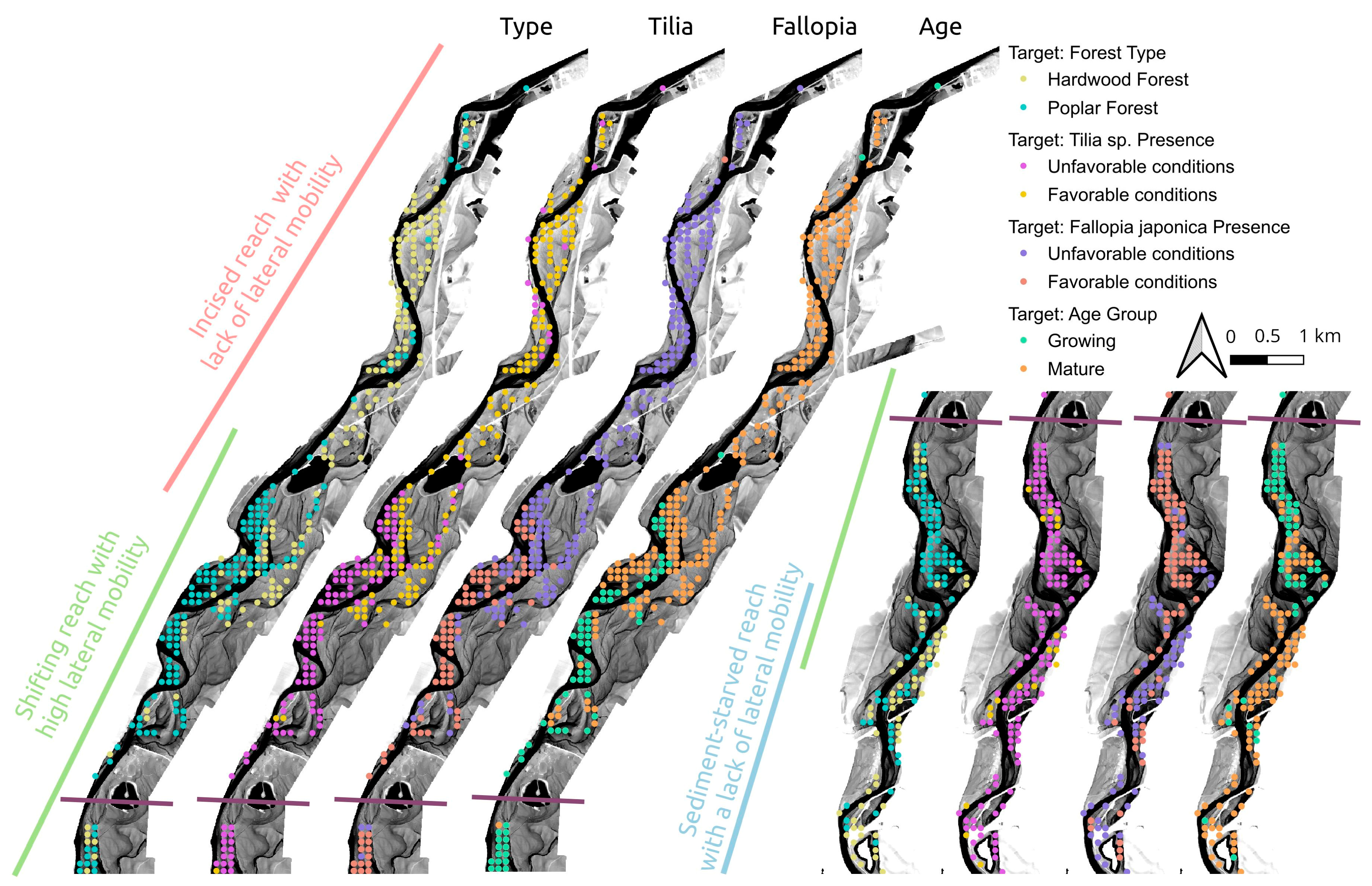
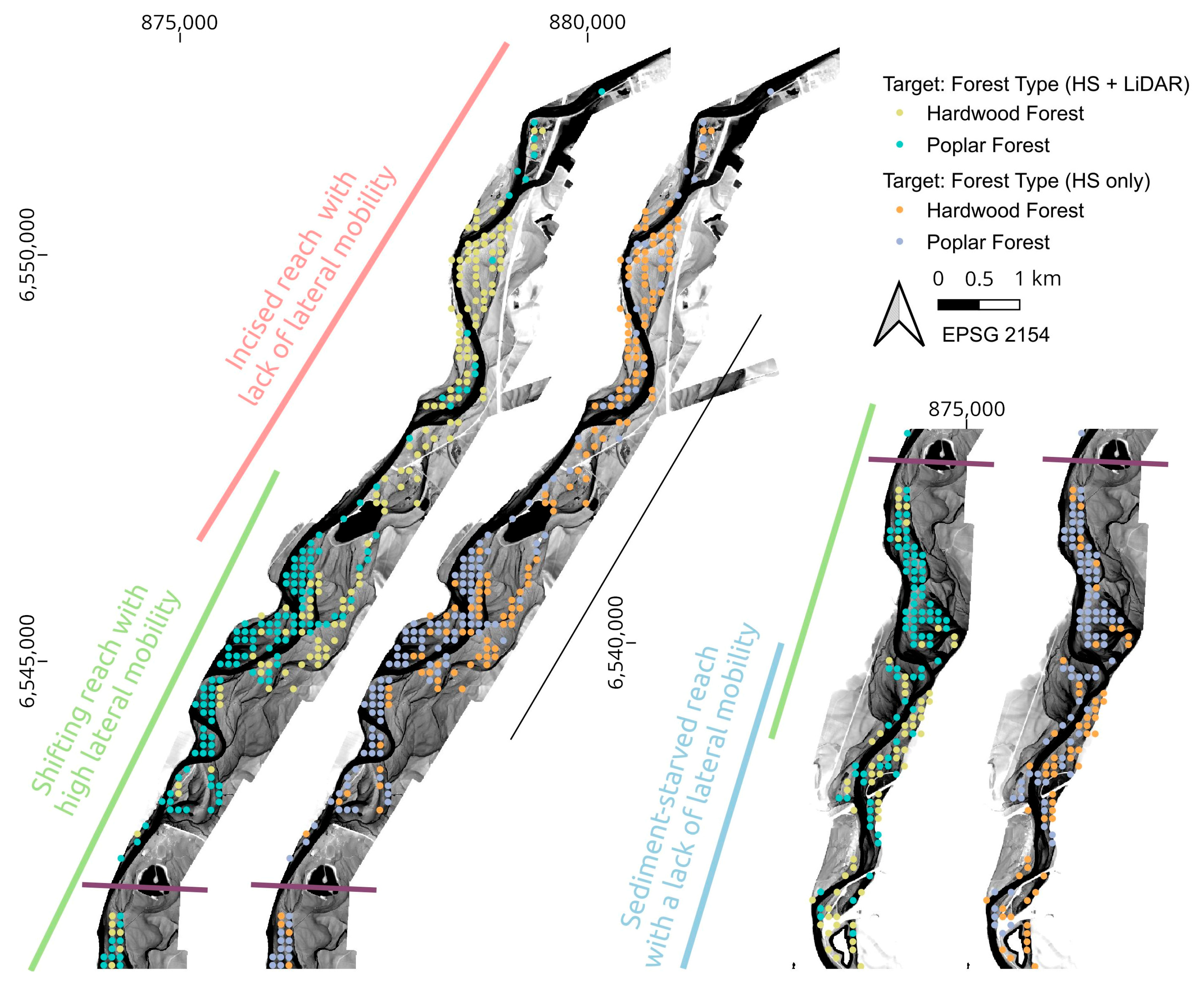
5.2.2. Mapping Indicators of Riparian Forest Connectivity across the Lower Ain River

Overall, the results from the classification offer a specific view of the degree of hydrological connectivity of the riparian forest. The age group classification shows the location of riparian forest plots that are still growing and have been rejuvenated after the construction of the Vouglans dam (≈50 years before the data acquisitions). The forest type shows the location of the typical pioneer forest, comprised mostly of poplar trees, and where it has started transitioning or has transitioned towards the post-pioneer hardwood forest because of a lack of forest rejuvenation. Finally, the presence of either Fallopia japonica or Tilia cordata inside a vegetation plot is an indicator of riparian forest plots that have good hydrological connectivity or that are dry, respectively. Furthermore, all of the classifications resulted in a similar spatial trend across the lower Ain River (Figure 13).
The incised reach located in the upstream portion of the study area is characterized by older vegetation patches, apart from a few exceptions near small gravel bars. These patches were mostly predicted to be post-pioneer hardwood forest plots, although a few plots were still predicted to be poplar forest plots, mostly those located near paleo-channels or extremely close in elevation to the river. In addition, the whole reach features unfavorable conditions for the development of Fallopia japonica, but favorable conditions for the development of Tilia cordata.
In the shifting reach, lateral mobility leads to the rejuvenation of the riparian forest and the presence of many forest plots that have not yet reached maturity, although some mature plots can be seen on more elevated or older riverbanks that have not yet been rejuvenated, such as in the Mollon Site (south), whose specific location can be found in Figure 3. Even though there is a diversity between mature and growing forest plots in this shifting reach of the river, most plots were predicted to be poplar forest plots, rather than post-pioneer hardwood forest plots (irrespective of whether they were predicted in one age group or the other), and were also mostly predicted as being favorable towards the implantation and growth of Fallopia japonica.
Finally, those plots located along the third geomorphic reach, referred to as the sediment-starved reach in this paper, were mostly mature vegetation plots because the lateral mobility of the river was constrained by morainic deposits. While, on the one hand, this element, coupled with the lack of favorable forest patches for Fallopia japonica, shows a low degree of hydrological connectivity, compared with forest patches from the shifting reach; on the other hand, the fact that the same forest patches are also predicted as being unfavorable for Tilia cordata suggests that the degree of hydrological connectivity is higher than that for plots in the incised reach, which would, therefore, be dryer. This degree of connectivity between that of the incised reach and that of the shifting reach would explain the equal division of forest patch predictions between poplar forest and post-pioneer hardwood forest.
All four classification targets generated maps demonstrating that the impact of channel incision on the riparian forest could be assessed by coupling LiDAR and hyperspectral data. However, using hyperspectral data alone can lead to extremely similar maps at the scale of the lower Ain River (Figure 14). Therefore, reflectance data alone were used to predict the upstream–downstream trend of hydrological connectivity of the riparian forest, and to discriminate between the incised and shifting sections of the river.

6. Discussion

Combining hyperspectral, LiDAR, and field data allowed for the analysis of the characteristics of the riparian forest of the lower Ain River, which is a forest featuring patches of varying ages due to rejuvenation that are distributed across reaches with different geomorphic features (high lateral mobility, constrained lateral mobility, and channel incision).
The topographic and sedimentological status of the riparian forest was investigated at a large scale along a 20-km river corridor, which highlighted both age (objective 1) and channel incision (objective 2) as drivers of change. Age led to a reduction in sedimentation processes as forest patches became more elevated and to development of forest soil leading to increased depth and available water capacity, which is in line with previous observations of young trees altering the topography of gravel bars [34]. Channel incision led to a decrease in patch connectivity at a given age, with an increase in plot elevation and a decrease in sedimentation, soil depth, and available water content.
Analysis of the field data showed that a transition from a pioneer forest consisting mainly of poplar trees towards a post-pioneer hardwood forest, from which poplars and other characteristic species of the riparian forest were absent, occurred with age, and this transition was more pronounced for plots affected by channel incision. For plots of the same age, channel incision leads to an increase in species preferring dry soil conditions, such as shrub species or Tilia sp., as is the case on the Drôme and Bès Rivers, where shrublands featured a higher relative elevation than post-pioneer units of the same age [35], or as observed by Dufour along the Magra River in Italy, where channel degradation also favored species adapted to dryer conditions [75].
Both age and patch connectivity were also drivers of change in the overall structure of the riparian forest and its reflectance. We found that LiDAR-derived height was able to predict the age of early pioneer communities up to 30 y.o., similar to the results of work that discriminated poplar developmental stages in Arizona [28]. However, in more mature patches, the structure of the vegetation was not found to be related to age and appeared to be more a function of forest connectivity and its associated shifts in species composition, as the vegetation structure was correlated with canopy water content and vegetation greenness.
Channel incision appeared to lead to a decrease in canopy greenness and water content, due to the resulting constraints on the availability of water resources, which suggests a sign of plant stress following incision, similar to the browning of riparian woodlands in California following a groundwater drop, due to a drought event [40].
The connectivity of forest patches was predicted through random forest classification targeting different indicators, such as the presence of species indicative of dryer soil conditions (objective 3). The accuracy of the classifications was higher than 80%, which is similar to or slightly lower than found in hyperspectral studies classifying species in non-riparian environments [53,54] or detecting the presence of Tamarisk sp. [76] in Southern California.
However, one of the limitations of this work that prevented attempts to directly map species was that it was restricted to forestry information in the form of vegetation plots covering a wide surface area in which multiple individuals of different species co-existed, which resulted in plots of mixed vegetation. Since successful classifications in mixed forests have been achieved with calibration data at the tree level [58,59] and tree crown detection from LiDAR data was achieved in a riparian environment in the Susa Valley of Italy [77], species mapping could be achievable in riparian forests.
Since all four classification targets achieved good results for the Ain River (including predicting the presence in the plot of Fallopia japonica, a species that cannot be seen at the canopy level) and led to similar maps showing the trends in hydrological connectivity of the lower Ain River, caution appears to be necessary when attempting to map species in riparian environments by remote sensing. The hyperspectral indexes selected by the random forest classifier were greenness and canopy water content, which can be indicative of water stress, rather than species. Therefore, it is possible that research work targeting the identification of invasive species using satellite data would produce a map of the forest patches that are more favorable to the growth and development of such species (which can also be of interest for scientists and stakeholders), rather than showing the actual presence of that species.
Therefore, future work should pay attention to the fact that differing degrees of hydrological connectivity, and the water stress that can result from them could interfere with classifications targeted at species detection in riparian environments. Detecting forest connectivity and mapping the impact of channel incision, as performed in this study, also provides useful data for researchers and stakeholders, because it can separate healthy riparian forest from dryer patches at the reach scale. This could lead to better management practices and help in prioritizing restoration actions by targeting dryer forest patches.
It seems possible to extract reproducible results on forest characteristics from LiDAR data, as documented in the previous literature. However, having only one hyperspectral campaign prevented us from assessing the impact of seasonality on the riparian vegetation signature and from knowing whether forest connectivity and health could be monitored from space by multispectral satellite data, such as that from Sentinel-2, or by hyperspectral data from satellites, such as PRISMA.
Not only are there seasonal differences in the reflectance between individuals of the same species [39] and between different species that do not have the same phenological windows [42], but the temperature and water levels are also seasonal. This study used data collected at the end of summer when the discharge of the Ain River was usually low and the temperature was high, which may bias the spectra towards the signature of hydrological connectivity and potentially plant stress.
In order to validate our hypothesis about hydrological connectivity and assess its impact on the spectral signature of riparian trees of the same species, in-field eco-physiological measurements of tree water stress would be necessary, and these could help target remote sensing surveys to the correct temporal and seasonal windows for mapping species and/or forest connectivity and health.

7. Conclusions

In this paper, riparian forest patches were studied by combining in-field surveys with LiDAR and hyperspectral data to better understand how the patches change through age and how they are affected by geomorphic changes, such as channel incision.
The topography underneath the forest patches was found to change with age, with increasing age leading to more elevated patches with a deeper soil that can store more water. However, forest patches in the incised reach of the Ain River were more elevated and featured shallower soils with less water retention capacity than those in non-incised reaches.
The composition of the forest was also found to change with age and the degree of hydrological connectivity. Older forest plots were transitioning towards post-pioneer environments, with this transition being more advanced for a particular age in forest patches located in the incised reach of the river. Channel incision also leads to the implantation of species preferring dryer conditions.
Although the forest grows with age, the heights of forest patches in the incised reach were found to be lower than those of patches in other reaches. In mature forest plots, the canopy structure correlated with hyperspectral indexes of greenness and canopy water content, suggesting that this difference could be due to higher water stress in the communities growing along the incised reach of the Ain River.
In addition to characterizing the impact of age and vertical connectivity on the riparian forest and its health, the datasets were used to attempt to predict forest connectivity from remotely sensed indicators generated from LiDAR and hyperspectral data, with random forest classification being used to target key species, the shift between the poplar forest and post-pioneer hardwood forest, and whether forest plots were still growing or mature.
The resulting forest maps highlighted the downstream–upstream gradient of hydrological connectivity along the studied section of the Ain River. Forest rejuvenation does not occur in the incised reach, and channel incision led to a more post-pioneer type hardwood forest, which is favorable to species liking dry conditions. In contrast, the shifting reach of the river, where fluvial dynamics occur, features a forest where rejuvenation processes are still ongoing and where older and mature patches can still feature the pioneer poplar forest typical of the Ain River, although they are more likely to also be favorable for the development of the invasive Japanese knotweed.
Our study highlights the potential of hyperspectral and LiDAR data for studying riparian forests and understanding the co-occurring processes of forest growth and impacts from anthropic changes, such as channel incision. The techniques could provide diagnostic tools to help differentiate healthy riparian forest from dryer patches that could warrant restoration actions. In addition, the possibility of using reflectance data alone for mapping the connectivity of riparian forests is promising for monitoring our forests and their responses to climate change and restoration actions. However, fully exploring the changes occurring in riparian forests along the two gradients of age and connectivity required good field data and information derived from LiDAR data and was a crucial first step for understanding the processes at play in our study site. Nevertheless, further research is needed to assess the reproducibility of our results and whether they could be obtained using low-cost and readily available multispectral data from satellites.

Author Contributions

Conceptualization, J.G., J.L., L.D., S.B. and H.P.; methodology, J.G.; software, J.G.; validation, J.G.; formal analysis, J.G.; investigation, J.G.; resources, J.L., L.D., S.B., K.M. and H.P.; data curation, J.G. and K.M.; writing—original draft preparation, J.G.; writing—review and editing, J.G., J.L., L.D., S.B., K.M. and H.P.; visualization, J.G.; supervision, J.L., L.D., K.M. and H.P.; project administration, J.L. and H.P.; funding acquisition, J.G., J.L., L.D., S.B. and H.P. All authors have read and agreed to the published version of the manuscript.

Funding

This research was funded by the Graduate School H2O’Lyon (ANR-17-EURE-0018) of the Université de Lyon (UdL), which is part of the program “Investissements d’Avenir” run by Agence Nationale de la Recherche (ANR). This research was also funded by the Rhône-Méditerranée-Corse Water Agency and partially funded by the “National Science Centre, Poland”, under contract agreement UMO-2017/25/B/ST10/0967. The hyperspectral data acquisition was funded by the European Facilities for Airborne Research (EUFAR).

Data Availability Statement

All the remote sensing data used in this paper are referenced on the data web catalog of the UMR 5600 EVS: https://elvis.ens-lyon.fr/geonetwork/srv/fre/catalog.search#/home (accessed on 18 December 2022). Please contact the authors for further details.

Acknowledgments

The authors would like to thank both EDF and the Université de Rennes (UMR 6118) for providing the LiDAR data used in this work, the Airborne Research and Survey Facilities of the Natural Environment Research Council (NERC-ARSF) for carrying out the hyperspectral data acquisition, and the French National Forests Office (ONF) and the Syndicat d’Ain Aval et de ses Affluents (SR3A) for one of the vegetation surveys used in this paper. The authors would also like to thank Cui Dandan, Zhi Zhang, Bianca Räpple, Fanny Arnaud, Christine Mouquet-Noppe, Vincent Warwrzyniak, Franck Perret, and Charles-Robin Gruel for their contributions to the fieldwork.

Conflicts of Interest

The authors declare no conflict of interest.

Appendix A. List of Indexes and Metrics Extracted from the LiDAR and Hyperspectral Data and Their Abbreviations

Appendix A.1. Narrowband Hyperspectral Indexes

1MSI
2NMDI
3WBI
4NDWI
5NDII
6CAI
7LCAI
8PSRI
9PRI
10MCARI
11MRENDVI
12MRESR
13MTVI
14MTVI2
15RENDVI
16TCARI
17TVI
18VREI1
19VREI2
20ARI1
21ARI2
22CRI1
23CRI2
24NDLI
25NDNI

Appendix A.2. Topographic Indexes Derived from LiDAR Data

1Elevation relative to low-flow water level (Detrend)
2Catchment area (CA)
3Catchment slope (CS)
4Modified catchment area (MCA)
5Topographic wetness index (TWI)
6Multiresolution index of ridge top flatness (MRRTF)
7Multiresolution index of valley bottom flatness (MRVBF)
8Direct insolation (DI)
9Diffuse insolation (DI.1)
10Total insolation (TI)
11Duration of insolation (DoI)
12Topographic position index (TPI)

Appendix A.3. Structural Indexes Derived from LiDAR Data

1Maximum height (zmax)
2Mean height (zmean)
3Entropy of height distribution (zentropy)
4Percentage of returns above zmean (pzabovemean)
55th percentile of height distribution (zq5)
610th percentile of height distribution (zq10)
715th percentile of height distribution (zq15)
820th percentile of height distribution (zq20)
925th percentile of height distribution (zq25)
1030th percentile of height distribution (zq30)
1135th percentile of height distribution (zq35)
1240th percentile of height distribution (zq40)
1345th percentile of height distribution (zq45)
1450th percentile of height distribution (zq50)
1555th percentile of height distribution (zq55)
1660th percentile of height distribution (zq60)
1765th percentile of height distribution (zq65)
1870th percentile of height distribution (zq70)
1975th percentile of height distribution (zq75)
2080th percentile of height distribution (zq80)
2185th percentile of height distribution (zq85)
2290th percentile of height distribution (zq90)
2395th percentile of height distribution (zq95)
24Cumulative percentage of returns in the 1st layer (zpcum1)
25Cumulative percentage of returns in the 2nd layer (zpcum2)
26Cumulative percentage of returns in the 3rd layer (zpcum3)
27Cumulative percentage of returns in the 4th layer (zpcum4)
28Cumulative percentage of returns in the 5th layer (zpcum5)
29Cumulative percentage of returns in the 6th layer (zpcum6)
30Cumulative percentage of returns in the 7h layer (zpcum7)
31Cumulative percentage of returns in the 8th layer (zpcum8)
32Cumulative percentage of returns in the 9th layer (zpcum9)
33Total intensity (itot)
34Max intensity (imax)
35Mean intensity (imean)
36Percentage of intensity returned by points classified as ground (ipground)
37Percentage of intensity returned below the 10th percentile (ipcumzq10)
38Percentage of intensity returned below the 30th percentile ipcumzq30
39Percentage of intensity returned below the 50th percentile ipcumzq50
40Percentage of intensity returned below the 70th percentile ipcumzq70
41Percentage of intensity returned below the 90th percentile ipcumzq90
42Percentage of intensity returned by 1st returns (p1th)
43Percentage of intensity returned by 2nd returns (p2th)
44Percentage of intensity returned by 3rd returns (p3th)
45Percentage of intensity returned by 4th returns (p4th)
46Percentage of intensity returned by 5th returns (p5th)
47Percentage of returns classified as ground per square meter (pground)
48Points per square meter (n)

References

  1. Naiman, R.J.; Decamps, H.; Pastor, J.; Johnston, C. The Potential Importance of Boundaries to Fluvial Ecosystems. J. N. Am. Benthol. Soc. 1988, 7, 289–306. [Google Scholar] [CrossRef]
  2. Naiman, R.J.; Decamps, H.; Pollock, M. The Role of Riparian Corridors in Maintaining Regional Biodiversity. Ecol. Appl. A Publ. Ecol. Soc. Am. 1993, 3, 209–212. [Google Scholar] [CrossRef] [PubMed]
  3. Riis, T.; Kelly-Quinn, M.; Aguiar, F.C.; Manolaki, P.; Bruno, D.; Bejarano, M.D.; Clerici, N.; Fernandes, M.R.; Franco, J.C.; Pettit, N.; et al. Global Overview of Ecosystem Services Provided by Riparian Vegetation. BioScience 2020, 70, 501–514. [Google Scholar] [CrossRef]
  4. Poole, G.C.; Berman, C.H. An Ecological Perspective on In-Stream Temperature: Natural Heat Dynamics and Mechanisms of Human-CausedThermal Degradation. Environ. Manag. 2001, 27, 787–802. [Google Scholar] [CrossRef]
  5. Roth, T.R.; Westhoff, M.C.; Huwald, H.; Huff, J.A.; Rubin, J.F.; Barrenetxea, G.; Vetterli, M.; Parriaux, A.; Selker, J.S.; Parlange, M.B. Stream Temperature Response to Three Riparian Vegetation Scenarios by Use of a Distributed Temperature Validated Model. Environ. Sci. Technol. 2010, 44, 2072–2078. [Google Scholar] [CrossRef] [PubMed]
  6. Wondzell, S.M.; Diabat, M.; Haggerty, R. What Matters Most: Are Future Stream Temperatures More Sensitive to Changing Air Temperatures, Discharge, or Riparian Vegetation? J. Am. Water Resour. Assoc. 2019, 55, 116–132. [Google Scholar] [CrossRef] [Green Version]
  7. Dosskey, M.G.; Vidon, P.; Gurwick, N.P.; Allan, C.J.; Duval, T.P.; Lowrance, R. The Role of Riparian Vegetation in Protecting and Improving Chemical Water Quality in Streams1. J. Am. Water Resour. Assoc. 2010, 46, 261–277. [Google Scholar] [CrossRef]
  8. Tabacchi, E.; Lambs, L.; Guilloy, H.; Planty-Tabacchi, A.-M.; Muller, E.; Décamps, H. Impacts of Riparian Vegetation on Hydrological Processes. Hydrol. Process. 2000, 14, 2959–2976. [Google Scholar] [CrossRef]
  9. Décamps, H. How a Riparian Landscape Finds Form and Comes Alive. Landsc. Urban Plan. 2001, 57, 169–175. [Google Scholar] [CrossRef]
  10. González del Tánago, M.; Martínez-Fernández, V.; Aguiar, F.C.; Bertoldi, W.; Dufour, S.; García de Jalón, D.; Garófano-Gómez, V.; Mandzukovski, D.; Rodríguez-González, P.M. Improving River Hydromorphological Assessment through Better Integration of Riparian Vegetation: Scientific Evidence and Guidelines. J. Environ. Manag. 2021, 292, 112730. [Google Scholar] [CrossRef]
  11. Francis, R.A.; Gurnell, A.M.; Petts, G.E.; Edwards, P.J. Survival and Growth Responses of Populus nigra, Salix elaeagnos and Alnus incana Cuttings to Varying Levels of Hydric Stress. For. Ecol. Manag. 2005, 210, 291–301. [Google Scholar] [CrossRef]
  12. Bravard, J.-P.; Amoros, C.; Pautou, G.; Bornette, G.; Bournaud, M.; Creuzé des Châtelliers, M.; Gibert, J.; Peiry, J.-L.; Perrin, J.-F.; Tachet, H. River Incision in South-East France: Morphological Phenomena and Ecological Effects. Regul. Rivers: Res. Manag. 1997, 13, 75–90. [Google Scholar] [CrossRef]
  13. Comiti, F.; Da Canal, M.; Surian, N.; Mao, L.; Picco, L.; Lenzi, M.A. Channel Adjustments and Vegetation Cover Dynamics in a Large Gravel Bed River over the Last 200 years. Geomorphology 2011, 125, 147–159. [Google Scholar] [CrossRef]
  14. Poff, N.L.; Olden, J.D.; Merritt, D.M.; Pepin, D.M. Homogenization of Regional River Dynamics by Dams and Global Biodiversity Implications. Proc. Natl. Acad. Sci. USA 2007, 104, 5732–5737. [Google Scholar] [CrossRef] [PubMed] [Green Version]
  15. Scott, M.L.; Lines, G.C.; Auble, G.T. Channel Incision and Patterns of Cottonwood Stress and Mortality along the Mojave River, California. J. Arid Environ. 2000, 44, 399–414. [Google Scholar] [CrossRef]
  16. Décamps, H.; Fortuné, M.; Gazelle, F.; Pautou, G. Historical Influence of Man on the Riparian Dynamics of a Fluvial Landscape. Landsc. Ecol. 1988, 1, 163–173. [Google Scholar] [CrossRef] [Green Version]
  17. O’Briain, R. Climate Change and European Rivers: An Eco-Hydromorphological Perspective. Ecohydrology 2019, 12, e2099. [Google Scholar] [CrossRef]
  18. Rivaes, R.; Rodríguez-González, P.M.; Albuquerque, A.; Pinheiro, A.N.; Egger, G.; Ferreira, M.T. Riparian Vegetation Responses to Altered Flow Regimes Driven by Climate Change in Mediterranean Rivers. Ecohydrology 2013, 6, 413–424. [Google Scholar] [CrossRef]
  19. Stella, J.C.; Rodríguez-González, P.M.; Dufour, S.; Bendix, J. Riparian Vegetation Research in Mediterranean-Climate Regions: Common Patterns, Ecological Processes, and Considerations for Management. Hydrobiologia 2013, 719, 291–315. [Google Scholar] [CrossRef]
  20. Pautou, G.; Girel, J. La Végétation de La Basse Plaine de l’Ain: Organisation Spatiale et Évolution. In Recherches Interdisciplinaires sur Les Écosystèmes de la Basse Plaine de l’Ain (France): Potentialités Évolutives et Gestion; Documents de Cartographie Ecologique; Laboratoire de biologie végétale: Grenoble, France, 1986; pp. 75–96. [Google Scholar]
  21. Planty-Tabacchi, A.-M.; Tabacchi, E.; Naiman, R.J.; Deferrari, C.; Décamps, H. Invasibility of Species-Rich Communities in Riparian Zones. Conserv. Biol. 1996, 10, 598–607. [Google Scholar] [CrossRef]
  22. Tabacchi, E.; Planty-Tabacchi, A.-M.; Salinas, M.J.; Décamps, H. Landscape Structure and Diversity in Riparian Plant Communities: A Longitudinal Comparative Study. Regul. Rivers Res. Manag. 1996, 12, 367–390. [Google Scholar] [CrossRef]
  23. Carbonneau, P.; Fonstad, M.A.; Marcus, W.A.; Dugdale, S.J. Making Riverscapes Real. Geomorphology 2012, 137, 74–86. [Google Scholar] [CrossRef]
  24. Carbonneau, P.E.; Piégay, H. Introduction: The Growing Use of Imagery in Fundamental and Applied River Sciences. In Fluvial Remote Sensing for Science and Management; John Wiley & Sons, Ltd.: Chichester, UK, 2012; pp. 1–18. [Google Scholar]
  25. Dufour, S.; Rodríguez-González, P.M.; Laslier, M. Tracing the Scientific Trajectory of Riparian Vegetation Studies: Main Topics, Approaches and Needs in a Globally Changing World. Sci. Total Environ. 2019, 653, 1168–1185. [Google Scholar] [CrossRef]
  26. Carbonneau, P.E.; Dietrich, J.T. Cost-Effective Non-Metric Photogrammetry from Consumer-Grade SUAS: Implications for Direct Georeferencing of Structure from Motion Photogrammetry. Earth Surf. Process. Landf. 2017, 42, 473–486. [Google Scholar] [CrossRef] [Green Version]
  27. Huylenbroeck, L.; Laslier, M.; Dufour, S.; Georges, B.; Lejeune, P.; Michez, A. Using Remote Sensing to Characterize Riparian Vegetation: A Review of Available Tools and Perspectives for Managers. J. Environ. Manag. 2020, 267, 110652. [Google Scholar] [CrossRef] [PubMed]
  28. Farid, A.; Goodrich, D.C.; Sorooshian, S. Using Airborne Lidar to Discern Age Classes of Cottonwood Trees in a Riparian Area. West. J. Appl. For. 2006, 21, 149–158. [Google Scholar] [CrossRef] [Green Version]
  29. Bertoldi, W.; Gurnell, A.M.; Drake, N.A. The Topographic Signature of Vegetation Development along a Braided River: Results of a Combined Analysis of Airborne Lidar, Color Air Photographs, and Ground Measurements. Water Resour. Res. 2011, 47, W06525. [Google Scholar] [CrossRef]
  30. Henshaw, A.J.; Gurnell, A.M.; Bertoldi, W.; Drake, N.A. An Assessment of the Degree to Which Landsat TM Data Can Support the Assessment of Fluvial Dynamics, as Revealed by Changes in Vegetation Extent and Channel Position, along a Large River. Geomorphology 2013, 202, 74–85. [Google Scholar] [CrossRef]
  31. Corenblit, D.; Steiger, J.; Charrier, G.; Darrozes, J.; Garófano-Gómez, V.; Garreau, A.; González, E.; Gurnell, A.M.; Hortobágyi, B.; Julien, F.; et al. Populus nigra L. Establishment and Fluvial Landform Construction: Biogeomorphic Dynamics within a Channelized River. Earth Surf. Process. Landf. 2016, 41, 1276–1292. [Google Scholar] [CrossRef]
  32. Husson, E. Images from Unmanned Aircraft Systems for Surveying Aquatic and Riparian Vegetation. PhD Thesis, Swedish University of Agricultural Sciences, Uppsala, Sweden, 2016. [Google Scholar]
  33. Vautier, F.; Corenblit, D.; Hortobágyi, B.; Fafournoux, L.; Steiger, J. Monitoring and Reconstructing Past Biogeomorphic Succession within Fluvial Corridors Using Stereophotogrammetry: Stereophotogrammetry. Earth Surf. Process. Landf. 2016, 41, 1448–1463. [Google Scholar] [CrossRef]
  34. Bywater-Reyes, S.; Wilcox, A.C.; Diehl, R.M. Multiscale Influence of Woody Riparian Vegetation on Fluvial Topography Quantified with Ground-Based and Airborne Lidar. J. Geophys. Res. Earth Surf. 2017, 122, 1218–1235. [Google Scholar] [CrossRef]
  35. Lallias-Tacon, S.; Liébault, F.; Piégay, H. Use of Airborne LiDAR and Historical Aerial Photos for Characterising the History of Braided River Floodplain Morphology and Vegetation Responses. Catena 2017, 149, 742–759. [Google Scholar] [CrossRef]
  36. Räpple, B.; Piégay, H.; Stella, J.C.; Mercier, D. What Drives Riparian Vegetation Encroachment in Braided River Channels at Patch to Reach Scales? Insights from Annual Airborne Surveys (Drôme River, SE France, 2005–2011). Ecohydrology 2017, 10, e1886. [Google Scholar] [CrossRef]
  37. Hortobágyi, B. Multi-Scale Interactions between Riparian Vegetation and Hydrogeomorphic Processes (The Lower Allier River). Doctoral Dissertation, Université Clermont Auvergne, Clermont-Ferrand, France, 2018. [Google Scholar]
  38. Laslier, M. Suivi Des Impacts d’un Arasement de Barrage Sur La Végétation Riveraine Par Télédétection à Très Haute Résolution Spatiale et Temporelle. Doctoral Dissertation, Université Rennes 2, Rennes, France, 2018. [Google Scholar]
  39. Milani, G.; Kneubühler, M.; Tonolla, D.; Doering, M.; Wiesenberg, G.L.B.; Schaepman, M.E. Remotely Sensing Variation in Ecological Strategies and Plant Traits of Willows in Perialpine Floodplains. J. Geophys. Res. Biogeosciences 2019, 124, 2090–2106. [Google Scholar] [CrossRef] [Green Version]
  40. Kibler, C.L.; Schmidt, E.C.; Roberts, D.A.; Stella, J.C.; Kui, L.; Lambert, A.M.; Singer, M.B. A Brown Wave of Riparian Woodland Mortality Following Groundwater Declines during the 2012–2019 California Drought. Environ. Res. Lett. 2021, 16, 084030. [Google Scholar] [CrossRef]
  41. Dufour, S.; Muller, E.; Straatsma, M.; Corgne, S. Image Utilisation for the Study and Management of Riparian Vegetation: Overview and Applications. In Fluvial Remote Sensing for Science and Management; John Wiley & Sons, Ltd.: Hoboken, NJ, USA, 2012; pp. 215–239. ISBN 978-1-119-94079-1. [Google Scholar]
  42. Michez, A.; Piégay, H.; Jonathan, L.; Claessens, H.; Lejeune, P. Mapping of Riparian Invasive Species with Supervised Classification of Unmanned Aerial System (UAS) Imagery. Int. J. Appl. Earth Obs. Geoinf. 2016, 44, 88–94. [Google Scholar] [CrossRef]
  43. Michez, A.; Piégay, H.; Toromanoff, F.; Brogna, D.; Bonnet, S.; Lejeune, P.; Claessens, H. LiDAR Derived Ecological Integrity Indicators for Riparian Zones: Application to the Houille River in Southern Belgium/Northern France. Ecol. Indic. 2013, 34, 627–640. [Google Scholar] [CrossRef]
  44. Demarchi, L.; Bizzi, S.; Piégay, H. Hierarchical Object-Based Mapping of Riverscape Units and in-Stream Mesohabitats Using LiDAR and VHR Imagery. Remote Sens. 2016, 8, 97. [Google Scholar] [CrossRef] [Green Version]
  45. Bizzi, S.; Piégay, H.; Demarchi, L.; Van de Bund, W.; Weissteiner, C.J.; Gob, F. LiDAR-Based Fluvial Remote Sensing to Assess 50–100-Year Human-Driven Channel Changes at a Regional Level: The Case of the Piedmont Region, Italy. Earth Surf. Process. Landf. 2019, 44, 471–489. [Google Scholar] [CrossRef]
  46. Roberts, D.; Roth, K.; Perroy, R. Hyperspectral Vegetation Indices. In Hyperspectral Remote Sensing of Vegetation; CRC Press: Boca Raton, FL, USA, 2011; pp. 309–327. [Google Scholar] [CrossRef]
  47. Gao, B. NDWI—A Normalized Difference Water Index for Remote Sensing of Vegetation Liquid Water from Space. Remote Sens. Environ. 1996, 58, 257–266. [Google Scholar] [CrossRef]
  48. Gitelson, A.; Merzlyak, M.N. Spectral Reflectance Changes Associated with Autumn Senescence of Aesculus Hippocastanum L. and Acer platanoides L. Leaves. Spectral Features and Relation to Chlorophyll Estimation. J. Plant Physiol. 1994, 143, 286–292. [Google Scholar] [CrossRef]
  49. Hunt, E.R.; Rock, B.N. Detection of Changes in Leaf Water Content Using Near- and Middle-Infrared Reflectances. Remote Sens. Environ. 1989, 30, 43–54. [Google Scholar] [CrossRef]
  50. Penuelas, J.; Frederic, B.; Filella, I. Semi-Empirical Indices to Assess Carotenoids/Chlorophyll-a Ratio from Leaf Spectral Reflectance. Photosynthetica 1995, 31, 221–230. [Google Scholar]
  51. Sims, D.A.; Gamon, J.A. Relationships between Leaf Pigment Content and Spectral Reflectance across a Wide Range of Species, Leaf Structures and Developmental Stages. Remote Sens. Environ. 2002, 81, 337–354. [Google Scholar] [CrossRef]
  52. Pascucci, S.; Pignatti, S.; Casa, R.; Darvishzadeh, R.; Huang, W. Special Issue “Hyperspectral Remote Sensing of Agriculture and Vegetation”. Remote Sens. 2020, 12, 3665. [Google Scholar] [CrossRef]
  53. Dalponte, M.; Bruzzone, L.; Gianelle, D. Tree Species Classification in the Southern Alps Based on the Fusion of Very High Geometrical Resolution Multispectral/Hyperspectral Images and LiDAR Data. Remote Sens. Environ. 2012, 123, 258–270. [Google Scholar] [CrossRef]
  54. He, K.S.; Rocchini, D.; Neteler, M.; Nagendra, H. Benefits of Hyperspectral Remote Sensing for Tracking Plant Invasions. Divers. Distrib. 2011, 17, 381–392. [Google Scholar] [CrossRef]
  55. Shoot, C.; Andersen, H.-E.; Moskal, L.M.; Babcock, C.; Cook, B.D.; Morton, D.C. Classifying Forest Type in the National Forest Inventory Context with Airborne Hyperspectral and Lidar Data. Remote Sens. 2021, 13, 1863. [Google Scholar] [CrossRef]
  56. Demarchi, L.; Kania, A.; Ciężkowski, W.; Piórkowski, H.; Oświecimska-Piasko, Z.; Chormański, J. Recursive Feature Elimination and Random Forest Classification of Natura 2000 Grasslands in Lowland River Valleys of Poland Based on Airborne Hyperspectral and LiDAR Data Fusion. Remote Sens. 2020, 12, 1842. [Google Scholar] [CrossRef]
  57. da Silva, A.R.; Demarchi, L.; Sikorska, D.; Sikorski, P.; Archiciński, P.; Jóźwiak, J.; Chormański, J. Multi-Source Remote Sensing Recognition of Plant Communities at the Reach Scale of the Vistula River, Poland. Ecol. Indic. 2022, 142, 109160. [Google Scholar] [CrossRef]
  58. Dutta, D.; Wang, K.; Lee, E.; Goodwell, A.; Woo, D.K.; Wagner, D.; Kumar, P. Characterizing Vegetation Canopy Structure Using Airborne Remote Sensing Data. IEEE Trans. Geosci. Remote Sens. 2017, 55, 1160–1178. [Google Scholar] [CrossRef]
  59. Richter, R.; Reu, B.; Wirth, C.; Doktor, D.; Vohland, M. The Use of Airborne Hyperspectral Data for Tree Species Classification in a Species-Rich Central European Forest Area. Int. J. Appl. Earth Obs. Geoinf. 2016, 52, 464–474. [Google Scholar] [CrossRef]
  60. Shendryk, I.; Broich, M.; Tulbure, M.G.; McGrath, A.; Keith, D.; Alexandrov, S.V. Mapping Individual Tree Health Using Full-Waveform Airborne Laser Scans and Imaging Spectroscopy: A Case Study for a Floodplain Eucalypt Forest. Remote Sens. Environ. 2016, 187, 202–217. [Google Scholar] [CrossRef]
  61. Rollet, A.J.; Piégay, H.; Dufour, S.; Bornette, G.; Persat, H. Assessment of Consequences of Sediment Deficit on a Gravel River Bed Downstream of Dams in Restoration Perspectives: Application of a Multicriteria, Hierarchical and Spatially Explicit Diagnosis. River Res. Appl. 2014, 30, 939–953. [Google Scholar] [CrossRef]
  62. Piégay, H.; Bornette, G.; Citterio, A.; Hérouin, E.; Moulin, B.; Statiotis, C. Channel Instability as a Control on Silting Dynamics and Vegetation Patterns within Perifluvial Aquatic Zones. Hydrol. Process. 2000, 14, 3011–3029. [Google Scholar] [CrossRef]
  63. Dufour, S. Contrôles Naturels Anthropiques de La Structure et de La Dynamique Des Forêts Riveraines. PhD Thesis, Université Jean Moulin Lyon III, Lyon, France, 2005. [Google Scholar]
  64. Dumas, S. Les Habitats Forestiers de La Basse Vallée de l’Ain: Étude et Analyse; Office National des Forêts: Saint Denis, France, 2004; p. 38. [Google Scholar]
  65. Dumas, S.; Perrin, V. Le Suivi de La Forêt Alluviale de La Basse Vallée de l’Ain: Inventaire de Niveau II de 2006; Office National des Forêts: Saint Denis, France, 2006; p. 66. [Google Scholar]
  66. Dumas, S. Inventaire Des Boisements Forestiers de La Basse Vallée de l’Ain; Office National des Forêts: Saint Denis, France, 2017; p. 39. [Google Scholar]
  67. Lejot, J.; Piégay, H.; Hunter, P.D.; Moulin, B.; Gagnage, M. Utilisation de la télédétection pour la caractérisation des corridors fluviaux: Exemples d’applications et enjeux actuels. Géomorphol. Relief Process. Environ. 2011, 17, 157–172. [Google Scholar] [CrossRef] [Green Version]
  68. Lague, D.; Feldmann, B. Topo-Bathymetric Airborne LiDAR for Fluvial-Geomorphology Analysis. In Remote Sensing of Geomorphology; Paolo Tarolli, S.M.M., Ed.; Developments in Earth Surface Processes; Elsevier: Amsterdam, The Netherlands, 2020; Volume 23, pp. 25–54. [Google Scholar]
  69. Roussel, J.-R.; Auty, D.; Coops, N.; Tompalski, P.; Goodbody, T.R.H.; Meador, A.S.; Bourdon, J.-F.; De Boissieu, F.; Achim, A. LidR: An R Package for Analysis of Airborne Laser Scanning (ALS) Data. Remote Sens. Environ. 2020, 251, 112061. [Google Scholar] [CrossRef]
  70. Roux, C.; Alber, A.; Bertrand, M.; Vaudor, L.; Piégay, H. “FluvialCorridor”: A New ArcGIS Toolbox Package for Multiscale Riverscape Exploration. Geomorphology 2015, 242, 29–37. [Google Scholar] [CrossRef]
  71. Conrad, O.; Bechtel, B.; Bock, M.; Dietrich, H.; Fischer, E.; Gerlitz, L.; Wehberg, J.; Wichmann, V.; Böhner, J. System for Automated Geoscientific Analyses (SAGA) v. 2.1.4. Geosci. Model Dev. 2015, 8, 1991–2007. [Google Scholar] [CrossRef] [Green Version]
  72. Vogelmann, J.E.; Rock, B.N.; Moss, D.M. Red Edge Spectral Measurements from Sugar Maple Leaves. Int. J. Remote Sens. 1993, 14, 1563–1575. [Google Scholar] [CrossRef]
  73. Hardisky, M.; Klemas, V. Smart, and The Influence of Soil Salinity, Growth Form, and Leaf Moisture on the Spectral Radiance of Spartina Alterniflora Canopies. Photogramm. Eng. Remote Sens. 1983, 48, 77–84. [Google Scholar]
  74. Wang, L.; Qu, J.J. NMDI: A Normalized Multi-Band Drought Index for Monitoring Soil and Vegetation Moisture with Satellite Remote Sensing. Geophys. Res. Lett. 2007, 34. [Google Scholar] [CrossRef]
  75. Dufour, S.; Rinaldi, M.; Piégay, H.; Michalon, A. How Do River Dynamics and Human Influences Affect the Landscape Pattern of Fluvial Corridors? Lessons from the Magra River, Central–Northern Italy. Landsc. Urban Plan. 2015, 134, 107–118. [Google Scholar] [CrossRef]
  76. Hamada, Y.; Stow, D.A.; Coulter, L.L.; Jafolla, J.C.; Hendricks, L.W. Detecting Tamarisk Species (Tamarix spp.) in Riparian Habitats of Southern California Using High Spatial Resolution Hyperspectral Imagery. Remote Sens. Environ. 2007, 109, 237–248. [Google Scholar] [CrossRef]
  77. Belcore, E.; Latella, M. Riparian Ecosystems Mapping at Fine Scale: A Density Approach Based on Multi-Temporal UAV Photogrammetric Point Clouds. Remote Sens. Ecol. Conserv. 2022, 8, 644–655. [Google Scholar] [CrossRef]
Figure 1. Map of the study site: the lower Ain River, France.
Remotesensing 15 00017 g001
Figure 2. Trajectories of the riparian forest based on surveys conducted by the French National Forestry Office. They distinguish an initial colonization and growing phase (by Salix sp. and Populus nigra) from later successional stages that are more mature, where the tree width of Populus nigra increases and post-pioneer species start appearing in the understory or overtake as the predominant species.
Remotesensing 15 00017 g002
Figure 3. Location of the vegetation plots along the study site.
Remotesensing 15 00017 g003
Figure 4. Overall methodology applied in this paper.
Remotesensing 15 00017 g004
Figure 5. Elevation of reach types, relative to low-flow water level and according to age for EVS plots (a) and ONF plots (b), and overbank sedimentation of reach types between 2008 and 2015 according to the age of EVS plots (c) and ONF plots (d).
Remotesensing 15 00017 g005
Figure 6. Soil depth measured by hand auger (a) and available water capacity (b) for ONF forest plots of a given age in all three geomorphic reaches.
Remotesensing 15 00017 g006
Figure 7. Percentage of pioneer species in vegetation plots according to plot age in the EVS survey (a) and the area of poplar trees in proportion to post-pioneer ash trees according to plot age in the ONF survey (b).
Remotesensing 15 00017 g007
Figure 8. Ranges of relative elevation at which certain species were present in the forest plots of the ONF survey, considering only forest plots older than 50 years.
Remotesensing 15 00017 g008
Figure 9. LiDAR cross-section showing the developmental stages of the pioneer poplar forest of the Ain River on the Chatillon site.
Remotesensing 15 00017 g009
Figure 10. Relationships between structure (maxima and standard deviation of height) and age for the EVS plots on the age gradient (a,c), and for the ONF plots (b,d).
Remotesensing 15 00017 g010
Figure 11. Greenness (a) and Leaf Water Content (b) indexes, according to the age of forest plots and their geomorphic reach.
Remotesensing 15 00017 g011
Figure 12. The fifteen variables with the strongest contributions to each of the random forest models when combining both LiDAR and hyperspectral data, ordered by mean decrease in gini.
Remotesensing 15 00017 g012
Figure 13. Spatial trends of riparian forest connectivity across the lower Ain River, according to the four random forest classifiers and their respective targets. (For coordinate references, see Figure 3 or Figure 14).
Remotesensing 15 00017 g013
Figure 14. Comparison of forest-type prediction between the map resulting from both LiDAR and hyperspectral data and the map resulting from only hyperspectral data.
Remotesensing 15 00017 g014
Table 1. Example remote sensing publications involving riparian forest with poplars and/or willows and the main focus of the studies.
ReferenceData TypeMulti-Date
Acquisition
Species
Identification
Structural
Information
Temporal DynamicsTopography and Hydrological
Connectivity
[28]LiDAR X
[29]RGB imagery + LiDAR X X
[30]Landsat imageryX X
[31]RGB imagery + photogrammetryX XXX
[32]RGB imagery X
[33]RGB imagery + photogrammetryX XXX
[34]LiDAR X X
[35]RGB imagery + LiDARX XXX
[36]RGB imagery + LiDARX XXX
[37]RGB imagery + LiDAR + photogrammetryX X X
[38]RGB imagery + LiDARXXXXX
[39]Hyperspectral imageryX X
[40]Hyperspectral imagery + Landsat imageryX XX
Table 2. Remote sensing datasets used in this study.
Type of DataYears of AcquisitionSpatial ResolutionSpectral Information
Aerial Photographs1945, 1954, 1963, 1971, 1980, 1991, 1996, 2000, 2005, 2009, 20120.5 × 0.5–1 × 1 mColor RGB imagery since 2000, black and white before
LiDAR20081.8 pts/m2NIR Laser, but only topographic points were available
LiDAR201518.6 pts/m2
per laser
NIR laser +
green laser
Hyperspectral20151 × 1 m361 spectral bands
(380–2500 nm)
Table 3. Measurements and observations recorded in the two forestry surveys.
Characteristic2015 Vegetation Plots
(EVS Lab)
2017 Vegetation Plots
(ONF Survey)
Species compositionXX
Tree diameter10 m radius
if diameter > 30 cm
5 m radius
if diameter > 7.5 cm
Tree height
(in 5-m classes)
10 m radius
if diameter > 30 cm
5 m radius
if diameter > 7.5 cm
Basal area X
Understory cover 5 m radius
Grass cover 5 m radius
Dead trees10 m radius5 m radius
if diameter > 30 cm
5 m radius
if diameter > 7.5 cm
Soil depthXX
Soil humidity X
Organic matterX
Age X
Table 4. Classification targets.
Classification TargetClassesSite Conditions
Age groupGrowing and matureIdentifies the presence of lateral mobility and forest rejuvenation
Forest typePoplar forest and hardwood forestThe poplar forest should be located in growing forest patches and in mature forest patches that are well-connected to the river
Fallopia japonicaPresence and absenceRequires a wet environment and well-connected forest patches
Tilia cordataPresence and absenceColonizes and grows on the driest forest patches
Table 5. Example species distributions from the vegetation survey conducted by the EVS laboratory along the vertical gradient (70 y.o.) for plots in both the shifting reach and incised reach.
Site and Plot NumberReachProportion of Tilia sp.Proportion of Shrub SpeciesPresence of Fraxinus excelsior
Mollon 1Shifting2%8%Present
Mollon 2Shifting0%0%Present
Martinaz 1Shifting10%10%Present
Martinaz 2Shifting6%9%Present
Cormoz 1Incised56%0%Absent
Cormoz 2Incised0%85%Absent
Bellegarde 1Incised0%0%Present
Bellegarde 2Incised0%0%Present
Vorgey 1Incised0%41%Present
Vorgey 2Incised78%0%Present
Table 6. The five hyperspectral indexes showing the strongest correlation with canopy height for plots older than 50 years, and their correlation coefficients with forest plots younger than 50 years, forest plots older than 50 years, and all forest plots located in the well-connected shifting reach.
Spectral IndexReferenceTargetR2 vs. Mean Height
(<50 y.o.)
R2 vs. Mean Height
(>50 y.o.)
R2 vs. Mean Height
(All Plots in the Shifting Reach)
ReNDVI[48]Greenness0.090.470.30
VREI1[72]Greenness0.110.520.33
NDII[73]Canopy water content0.210.490.33
NDMI[74]Canopy water content0.200.470.31
MSI[49]Canopy water content0.210.490.33
Table 7. Class error for each of the four random forest classifiers, according to the data used in the classifier–LiDAR and/or hyperspectral (HS). For each class, 50 plots were used to train the classifier.
Classification TargetClassClass Error
LiDAR + HS
Class Error
LiDAR Only
Class Error
HS Only
Age groupGrowing
(<50 y.o.)
18%24%20%
Mature
(>50 y.o.)
16%16%28%
Forest typePoplar forest14%18%20%
Hardwood forest12%16%18%
Presence of Fallopia japonicaPresent20%20%26%
Absent16%14%28%
Presence of Tilia cordataPresent20%36%26%
Absent18%28%24%
Table 8. Class error for each of the four random forest classifiers (HS + LiDAR) once the random forest classifier was used to predict classes for each of the forest plots, instead of only the training data. The total number of plots was lower for the Forest Type classification target, due to the definition of each class (>75% black poplar or European ash trees in the plot), not including all forest plots.
Classification TargetClassPredicted A.Predicted B.Class ErrorMean Error
Age group(A.) Growing
(<50 y.o.)
841918.5%13.5%
(B.) Mature
(>50 y.o.)
282819%
Forest type(A.) Poplar forest1201712%11%
(B.) Hardwood forest87210%
Presence of Fallopia japonica(A.) Present7667.5%12%
(B.) Absent5327716%
Presence of Tilia cordata(A.) Present9699.5%17%
(B.) Absent7523224.5%
Table 9. Forest type of each vegetation plot according to the ONF survey and the number of plots of each type classified in each class of the four random forest classifications.
Forest Type (ONF)Age GroupForest TypeFallopia japonicaTilia cordata
GrowingMaturePoplarHardwoodPresentAbsentPresentAbsent
Early pioneer forest170161152018
Rapid growth series32356254720661
Slow growth series2222291521231529
Mature poplar forest with an understory21225668171078143
Post-pioneer hardwood forest688138115795935
Others2937363036301056
Disclaimer/Publisher’s Note: The statements, opinions and data contained in all publications are solely those of the individual author(s) and contributor(s) and not of MDPI and/or the editor(s). MDPI and/or the editor(s) disclaim responsibility for any injury to people or property resulting from any ideas, methods, instructions or products referred to in the content.

