Enhanced CNN Classification Capability for Small Rice Disease Datasets Using Progressive WGAN-GP: Algorithms and Applications

Abstract

An enhancement generator model with a progressive Wasserstein generative adversarial network and gradient penalized (PWGAN-GP) is proposed to solve the problem of low recognition accuracy caused by the lack of rice disease image samples in training CNNs. First, the generator model uses the progressive training method to improve the resolution of the generated samples step by step to reduce the difficulty of training. Second, to measure the similarity distance accurately between samples, a loss function is added to the discriminator that makes the generated samples more stable and realistic. Finally, the enhanced image datasets of three rice diseases are used for the training and testing of typical CNN models. The experimental results show that the proposed PWGAN-GP has the lowest FID score of 67.12 compared with WGAN, DCGAN, and WGAN-GP. In training VGG-16, GoogLeNet, and ResNet-50 with PWGAN-GP using generated samples, the accuracy increased by 10.44%, 12.38%, and 13.19%, respectively. PWGAN-GP increased by 4.29%, 4.61%, and 3.96%, respectively, for three CNN models over the traditional image data augmentation (TIDA) method. Through comparative analysis, the best model for identifying rice disease is ResNet-50 with PWGAN-GP in X2 enhancement intensity, and the average accuracy achieved was 98.14%. These results proved that the PWGAN-GP method could effectively improve the classification ability of CNNs.

1. Introduction

Rice is one of the most important food crops worldwide, especially in Asian countries, where it plays a crucial role in diets. According to statistics, more than 3 billion people rely on rice as their primary source of food, and rice production accounts for nearly 20% of the world’s total grain output. Additionally, rice is a major export commodity for many countries and regions and has significant impacts on local economies and trade [1]. Rice disease is one of the main factors affecting the high quality, efficiency, and yield of rice, so the recognition of rice diseases is an important method to protect food security.

The traditional method of rice disease recognition relies on visual observation and monitoring by plant protection specialists. However, this method requires experienced rice specialists, and long periods of monitoring are costly on large farms. The shortage of rice specialists, especially in developing countries, prevents effective and timely rice disease control.

With the development of artificial intelligence technology, researchers at home and abroad have successfully applied machine learning methods to the automatic recognition and identification of crop diseases. For example, image processing-based techniques have been used for rice disease detection and recognition with high recognition accuracy [2,3] involving support vectors [4,5], k-Nearest Neighbor [6], and decision trees [7]. Nevertheless, these methods have disadvantages, such as difficulties in implementation for large-scale training samples and solving multiple classification issues and sensitivity to the selection of parameters, which hinder the further improvement of the recognition effect. Significant breakthroughs in deep learning have been achieved with better results in recent years, which include convolutional neural (CNNs) networks [8,9] and migration learning [4,10] for image recognition.

Recently, deep learning has become a key technology for big data intelligence [11] and has been successfully applied to tasks of plant disease identification and classification. Compared with classical machine learning methods, deep learning has a more complex model structure with more powerful feature extraction capabilities. In [12], depthwise separable convolution was proposed for crop disease detection. Experimentally tested on a subset of the PlantVillage dataset, Reduced MobileNet achieved a classification accuracy of 98.34%, with a lower number of parameters than VGG and MobileNet. In [13], aiming at low power consumption and low performance of small devices, a depth-wise separable convolution (DSC)-based PLD (DSCPLD) recognition framework was proposed, which was tested on rice disease datasets, and the accuracy of using S-modified MobileNet and F-modified MobilNet reached 98.53% and 95.53%, respectively. In [4], the model for the classification of rice leaf disease images by ResNet-50 combined with the SVM method achieved an F1 score of 98.38%. In [14], to improve the accuracy of existing rice disease diagnosis, VGG-16 and GooLeNet models were used to train on a dataset of three painless species of diseases, and the experimental results showed that the average classification accuracies of VGG-16 and GoogLeNet were 92.24% and 91.28%, respectively. In [15], the authors constructed a novel rice blast recognition method based on CNN to identify 90% of diseased leaves and 86% of healthy leaves, respectively. Although the above methods achieve accurate recognition of rice diseases, deep learning techniques need to include large datasets that satisfy various criteria to obtain better recognition results. Note that using limited image datasets for training can lead to the overfitting of model training [16]. That is to say, training dataset size has a large impact on deep learning-based disease recognition methods, and their performance will be severely degraded in the case of small samples, uneven data distribution, etc. [17,18].

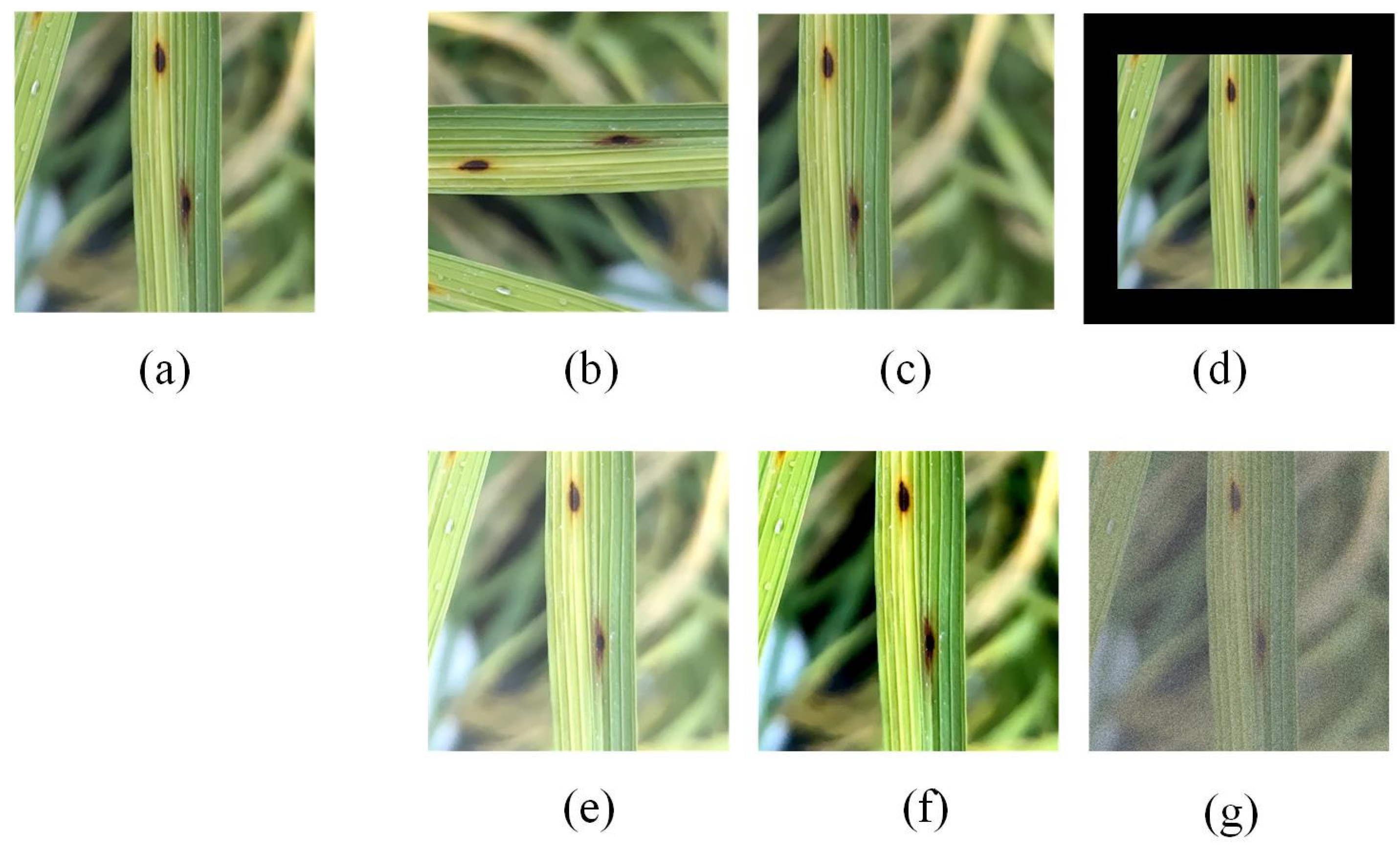
A strategy to solve the data shortage is to convert the original data to generate artificial data, which is usually called data augmentation. Data augmentation is achieved by executing geometric transformations, noise addition, interpolation, color transformation, and other operations on the original data. Common structures in convolutional neural networks include pooling layers, strided convolutions, and downsampling layers. When the position of the input image changes, the output tensor may change drastically. Therefore, convolutional neural networks may misclassify images that have undergone image processing transformations. This type of transformation can be used to enhance small sample image datasets. However, this data augmentation method does not increase the diversity of image features in the original dataset but only exploits the design flaw of convolutional neural networks [19]. Methods based on deep learning provide an effective and powerful way to learn the implicit representation of data distribution. Inspired by the zero-sum game in game theory, the Generative Adversarial Networks (GAN) model has been proposed in [20], which can learn how to approach the true distribution of data and has powerful capabilities in image generation. The original GAN suffers from the problems of difficult convergence, training, and control of the model. 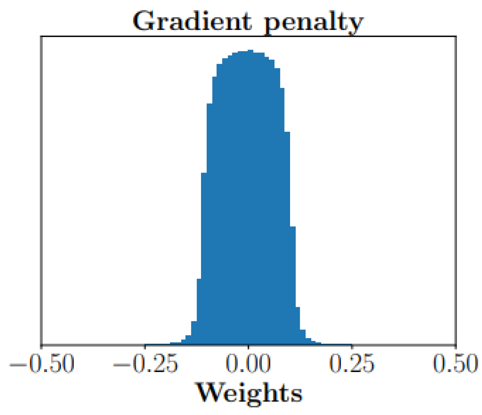To deal with these problems, the Wasserstein Generative Adversarial Network (WGAN) has been proposed in [21] to solve the difficulty of training the original GAN. WGAN training is more stable and theoretically solves the pattern collapse and the gradient disappearance. Whereas WGAN causes issues such as gradient explosion when generating data due to direct weight cropping, which makes the model training unstable. Wasserstein Generative Adversarial Network with Gradient Penalized (WGAN-GP) was developed in [22], a generative adversarial network that controls the gradient by gradient penalty to settle the matters of gradient explosion and pattern collapse.

At present, GAN has been employed effectively in the field of data enhancement. A method has been put forward in [23] based on deep learning for tomato disease diagnostics that uses the conditional generative adversarial network (CGAN) to produce synthetic images of tomato plant leaves. The recognition accuracy of this method in the classification of tomato leaf images into 5, 7, and 10 categories is 99.51%, 98.65%, and 97.11%, respectively. An infrared image-generation approach was designed in [24] depending on CGAN. This method can generate high-quality and reliable infrared image data. In [25], a model combining CycleGAN and U-net has been constructed and applied to a small dataset of tomato plant disease images. The results show that the model is better than the original CycleGAN. A fault recognition mechanism was presented in [26] for bearing small samples based on InfoGAN and CNN. The extracted time-frequency image features are input into InfoGAN for training to expand the data. Tested on the CWRU dataset, the results show that this method is better than other algorithms and models. In [27] a strategy was raised relying on a WGAN combined with a DNN. The cancer image is expanded by GAN to improve the classification accuracy and generalization of DNN. The results show that the classification accuracy of DNN using WGAN is the highest in comparison with other methods. CycleGAN has been put to use in [28] to retreat the CT segmentation task domain dataset for enhancement. The results display that the Dice score on the kidney increases from 0.09 to 0.66, and the effect is significant, while the improvement is small on the liver and spleen. However, WGAN-GP is still not effective at generating high-resolution images. Therefore, Tero Karras proposed Progressive GAN (ProGAN) in [29], a growing GAN-derived model, which generates very low-resolution images first, and then gradually increases the generated resolution during training to generate high-resolution images stably. In [30], a Dual GAN was proposed for generating high-resolution images of rice disease, which is used in the field of data enhancement. Dual GAN uses WGAN-GP to generate rice disease images, and Optimized-Real-ESRGAN is used to improve image resolution. The experimental results show that the accuracy of ResNet-18 and VGG-11 is improved by 4.57% and 4.1%, respectively. In [31], a novel neural network-based hybrid model (GCL) is proposed. CGL includes GAN for data enhancement, CNN for feature extraction, and LSTM for rice disease image classification. The experimental results show that the proposed method can achieve 97% accuracy for disease classification. In [32], a new convolutional neural network was proposed for the identification of three rice leaf diseases, using a GAN-based technique to augment the dataset. The experimental results showed that the proposed method achieved an accuracy of 98.23%. The above studies can show that GAN application is effective for data enhancement in small sample datasets, but the resolution and stability of the current generation are yet to be improved.

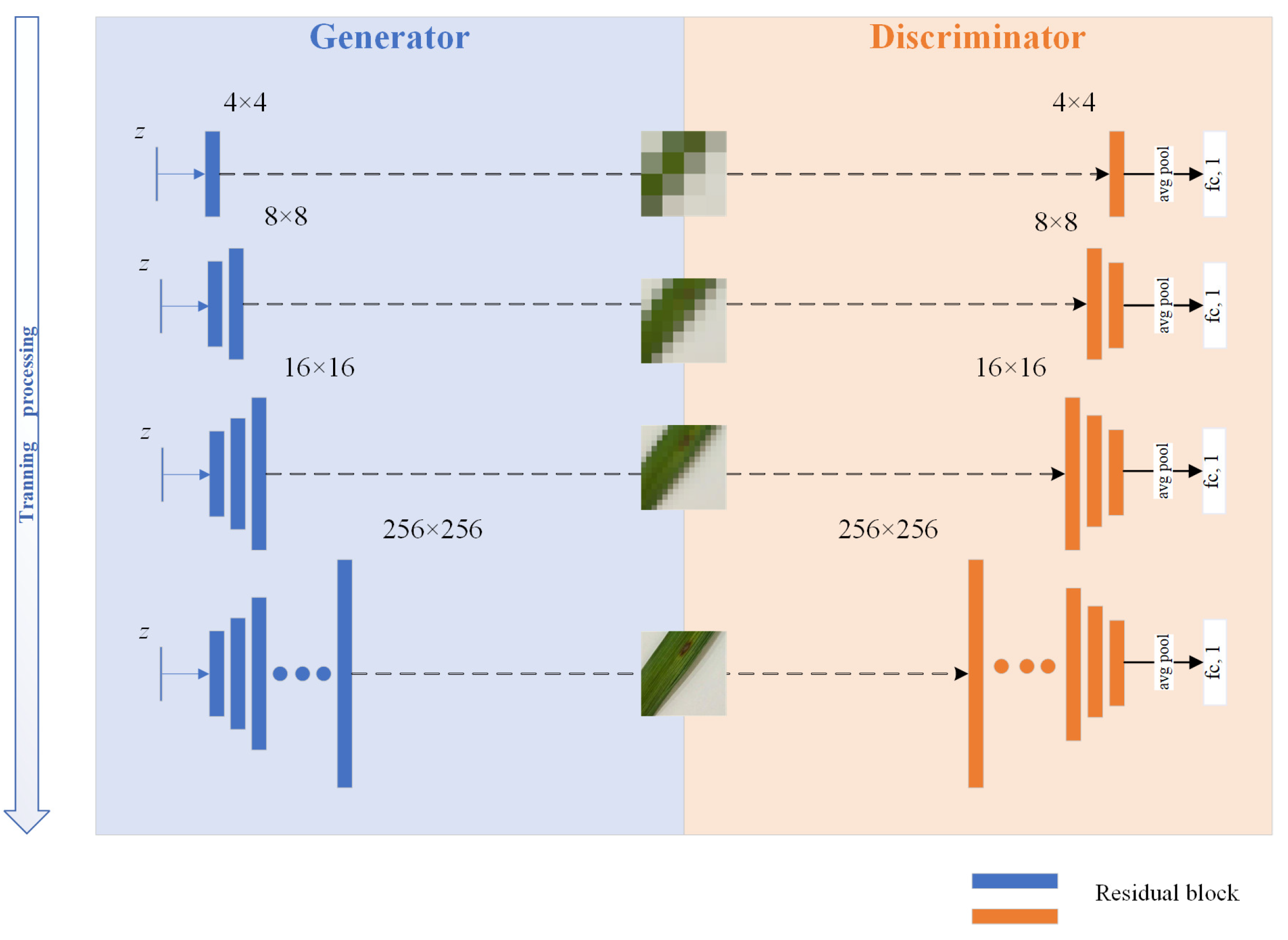
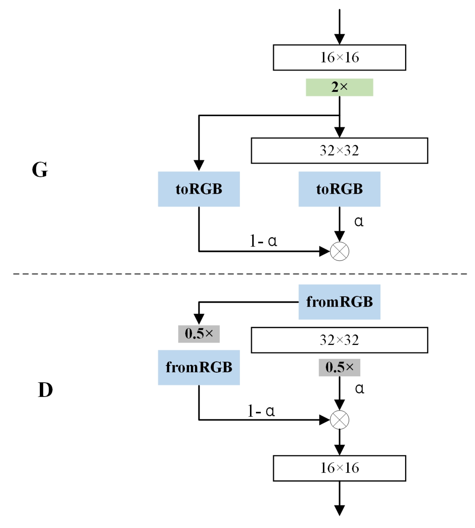
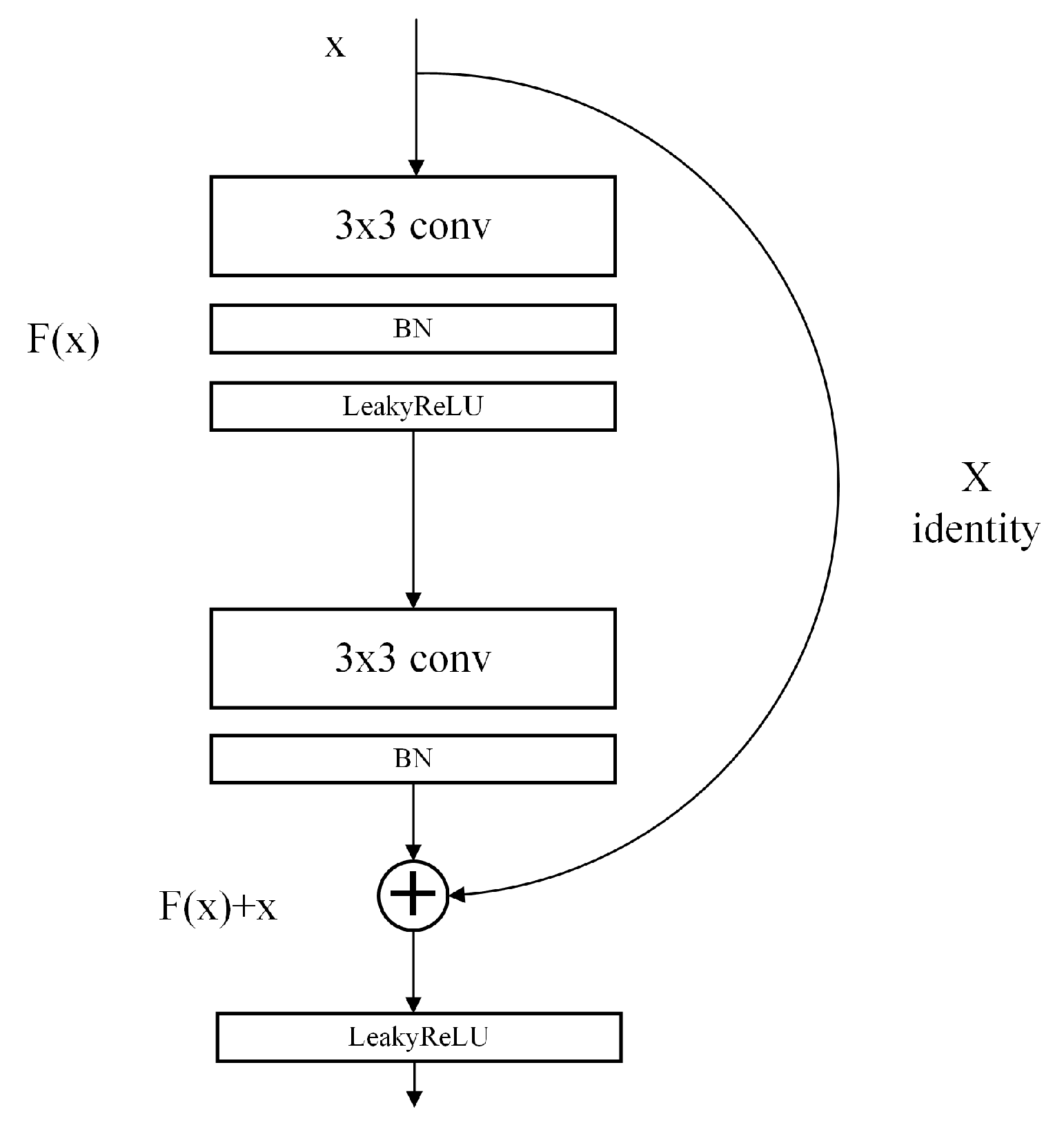
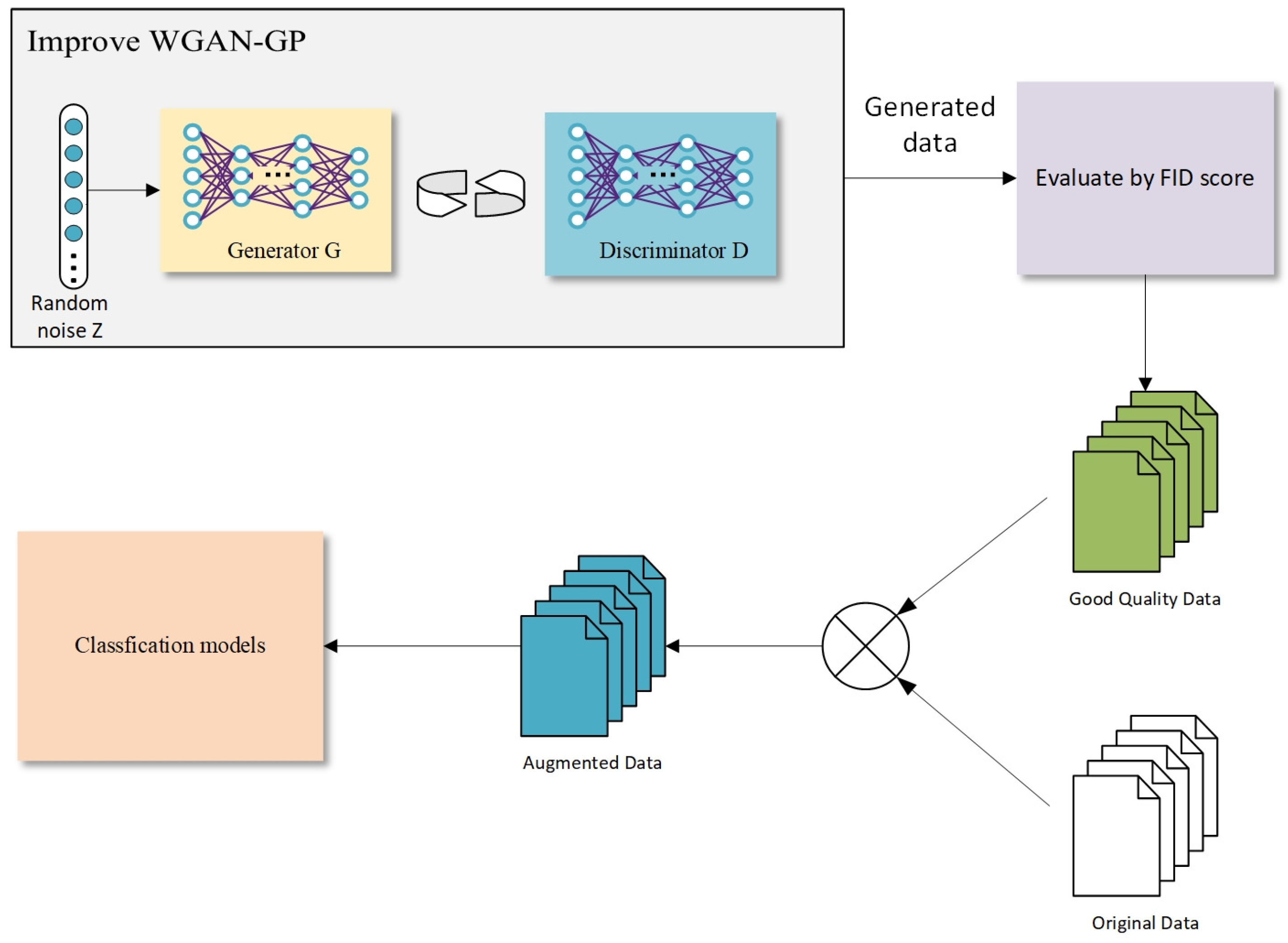
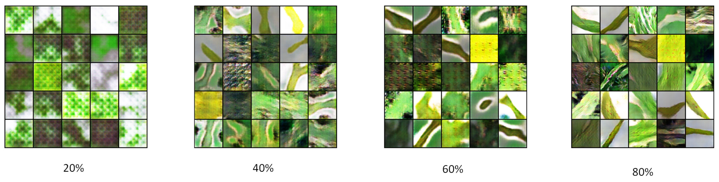
To alleviate the lack of image data on rice diseases, we introduce a Progressive WGAN-GP, which is based on the WGAN-GP model and combines a progressive training method. This model is applied to rice disease image data augmentation to increase the accuracy of the recognition model in small-sample datasets. By analyzing the three diseases in the collected dataset as well as the open-source dataset, the experimental results show that the method has good robustness and generalization ability and has a fine recognition effect under small sample conditions. The main contributions of this paper are twofold. (1) The progressive training method is introduced into the WGAN-GP model. In the field of rice disease image generation, the generation performs better than WGAN-GP, WGAN, and Deep convolutional GAN (DCGAN). (2) The experimental results show that the PWGAN-GP method can not only generate high-quality images of rice diseases but also apply the generated images to the CNNs training by blending the dataset with real images, which can improve the performance of CNNs, and obtain a higher recognition accuracy than other methods.

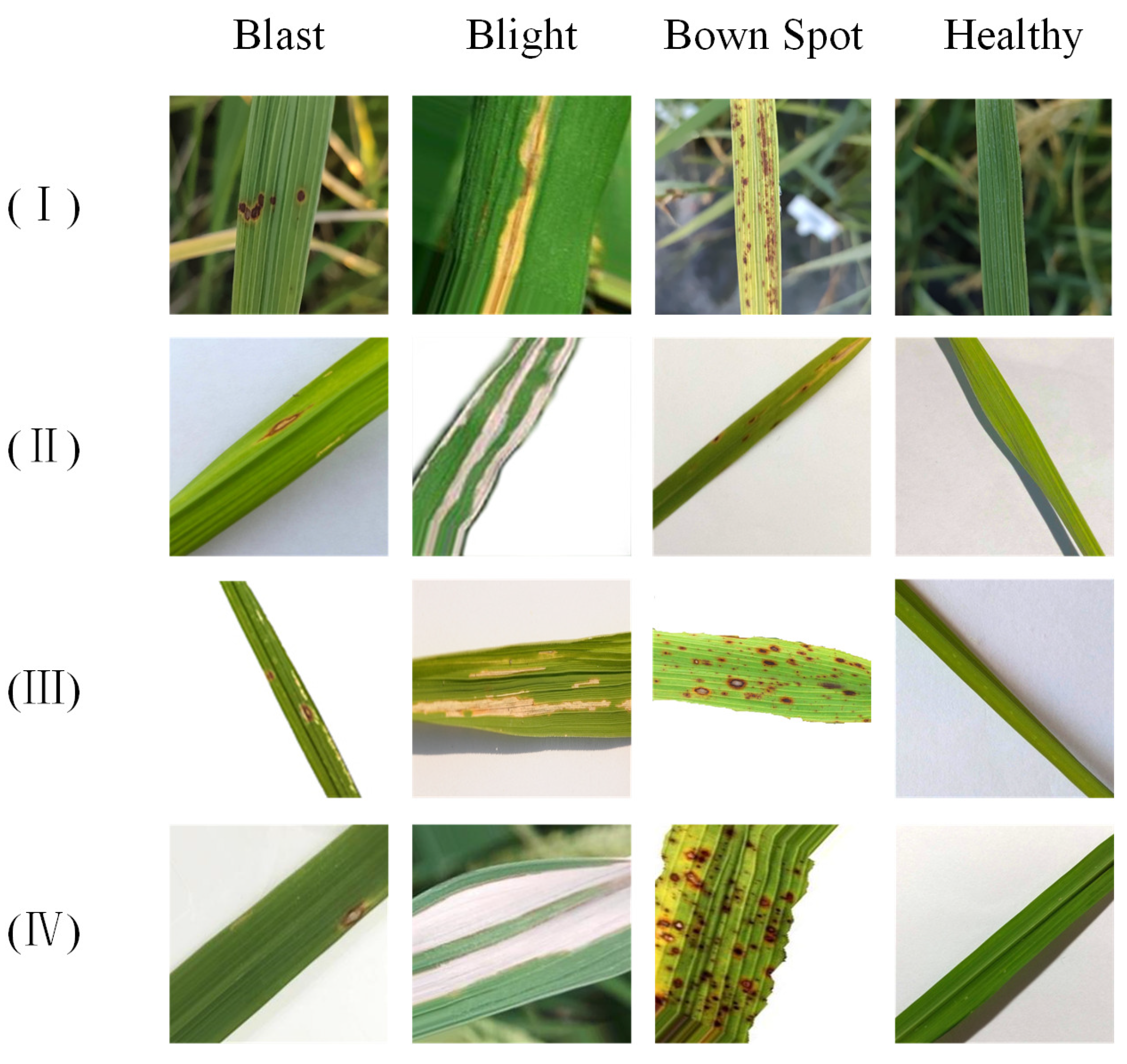
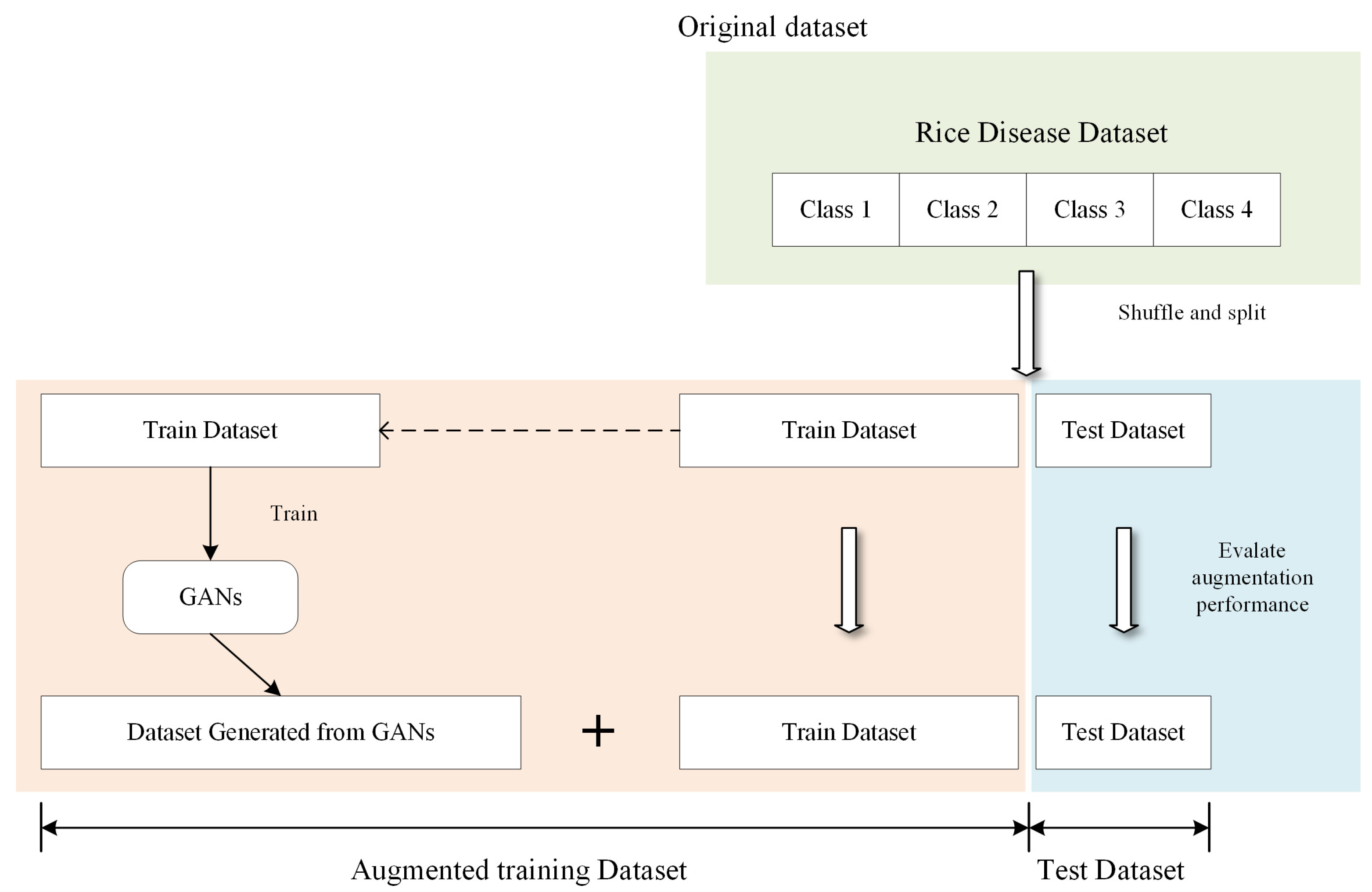
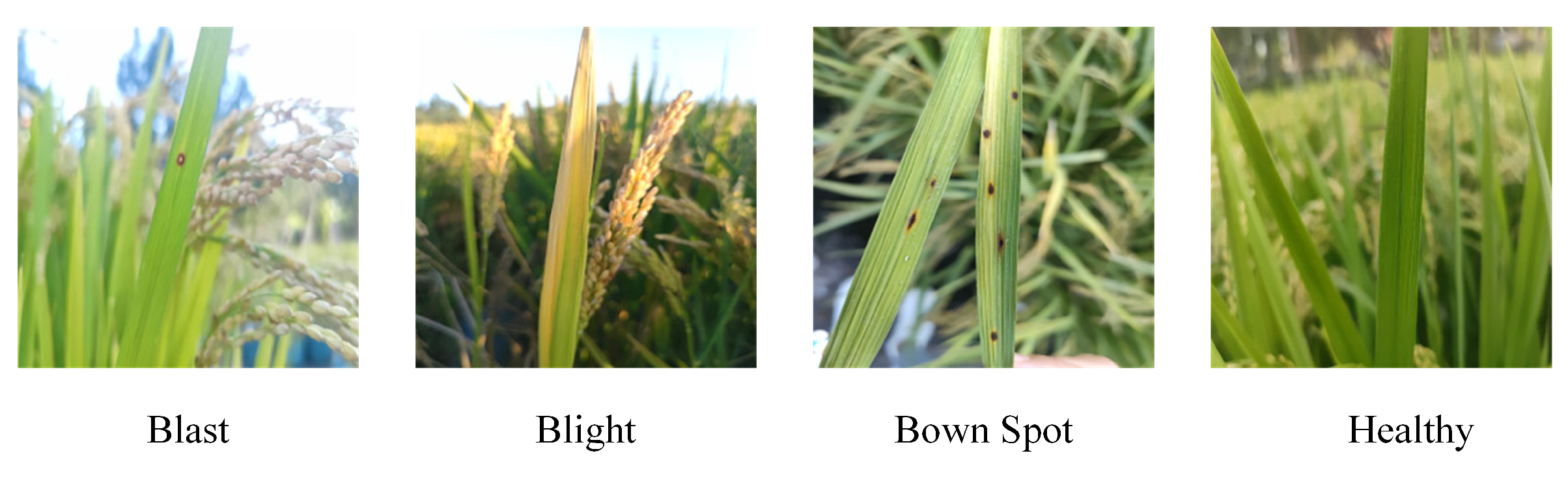
The remainder of this paper is organized as follows. In Section 2, we describe the source and the pre-processing of the data. Section 3 presents the theory related to PWGAN-GP. Section 4 describes the experimental setup of the PWGAN-GP for the application problem of rice disease image generation as well as recognition. Section 5 analyzes the experimental data of image generation and the comparison with other methods. Conclusions are given in Section 6.

2. Dataset

The image dataset used in this paper is shown in Figure 1. The rice disease image (I) is obtained from an experimental farm field at Heilongjiang Bayi Agricultural University. The device used to capture these rice images is a Redmi K30 Pro phone. The image dataset includes rice leaf blast, rice leaf blight, rice leaf brown spot, and healthy rice leaf to increase the diversity of rice disease image samples that are captured separately under different cycles of rice growth, weather conditions, and lighting conditions. The rice disease image datasets (II) [33], (III) [34], and (IV) [35] are from open-source databases available on the web. Database (II) contains 3355 images with 4 categories and an image resolution of 2798 × 2798 pixels; database (III) contains 120 images with 3 categories and an image resolution of 3081 × 897 pixels, and database (IV) contains 2800 images with 5 categories and an image resolution of 256 × 256 pixels. Since the open-source database contains a variety of categories of images, this experiment eliminates the images whose categories are not consistent with the research direction of this paper.

The dataset for this experiment consists of four sources, each with a high resolution from different sources, and in addition, there are differences in the methods of acquisition, which result in a non-uniform style of the dataset. Therefore, data pre-processing of the dataset is required. Duplicate, blurred, and images with insignificant disease characteristics are removed from the dataset. The number of categories in the pre-processed image dataset is shown in

Table 1. Details of the rice leaf disease dataset.

Categories	Numbers
Blast	1654
Brown Spot	1570
Blight	1396
Healthy	2563

.

The workflow of the process of data segmentation and augmentation is shown in Figure 2. We randomly shuffled the order of the original dataset and split 80% of the image samples as the training set for data augmentation and image recognition, while the remaining 20% of the image samples served as the test set for an independent performance evaluation of the data-augmented image recognition. It is important to note that the data in the test set do not participate in the data augmentation phase in order to ensure the fairness of the test. The detailed numbers of training and test sets are shown in

Table 2. Details of the rice leaf disease train and test dataset.

Categories	Train Dataset	Test Dataset
Blast	1323	331
Brown Spot	1256	314
Blight	1116	280
Healthy	2050	513

.

3. Methodology

3.1. GAN

GANs can be trained to generate high-quality images by learning the data distribution from the training set. GANs consist of two parts, one is the generator (G), and the other is the discriminator (D). The generator accepts the noise vector and generates samples. Then generates samples and real samples together to input into the discriminator, which needs to distinguish the real samples from the generated samples accurately. In the process of confrontation between the two models, the generated samples will be more realistic. At the same time, the discriminator’s discriminatory ability will be enhanced. The generator and discriminator will eventually game each other to reach the state of Nash equilibrium [20]. Because the samples generated by the GAN belong to the same labeled class as the original samples, they can be used for image dataset expansion. The objective function of the GAN is shown in Equation (1).

$$\begin{array}{c}\hfill \underset{G}{min}\underset{D}{max}V(D,G)=E_{x\sim p_{data\left(x\right)}}\left[log\left(D\left(x\right)\right)\right]+\\ \hfill E_{z\sim p_{\theta }\left(z\right)}\left[log(1-D\left(G\left(z\right)\right))\right]\end{array}$$

(1)

where $p_{data\left(x\right)}$ is the probability distribution of the real image and $\theta \left(z\right)$ is the input noise distribution of G. G and D fight against each other, with G continuously improving its ability to capture the true sample distribution and generate higher-quality images, and D improving its ability to discriminate the generated images. The original GAN has been shown to provide a more realistic output compared to other generative image algorithms.

However, there are three major problems with the original GAN as follows: (1) the loss function values of the generative and discriminant models are unstable during training, which indirectly leads to the instability of the generated images; (2) the original GAN architecture is prone to pattern collapse, where the generative model finds a limited range of samples from the original data that may result in the discriminator not being able to continue being effectively trained. In addition, the images generated by the generator lack diversity; and (3) adjusting the hyperparameters of the traditional GAN makes it very difficult to make the model converge.

3.2. WGAN

In [21], the theory related to Jensen-Shannon has been analyzed, which concludes that it is not reasonable to use Jensen-Shannon to measure the distance of disjoint parts between distributions. To improve the quality of the images generated by GAN, instead of using Jensen-Shannon, it is pointed out to use the Wasserstein distance measure as the distance between the generated data and the real data distribution. The definition of the Wasserstein distance is shown in Equation (2).

$$W(P_r,P_g)=\underset{\gamma \in \prod (P_r,P_g)}{inf}{E}_{(x,y)\sim \gamma }\left[∥x-y∥\right]$$

(2)

where $P_r$ is the distribution of the real data, $P_g$ is the distribution of the generated data, and $\gamma \in \prod (P_r,P_g)$ is the joint distribution of $P_r$ and $P_g$. The loss function of WGAN is shown in Equation (3).

$$L\left(D\right)=E_{z\sim P_z}\left[f_w\left(G\left(z\right)\right)\right]-E_{x\sim P_x}\left[f_w\left(x\right)\right]$$

(3)

where z is the input noise and x is the real input image. $G\left(z\right)$ is the image generated by the received noise as the input of the generator. $E_{z\sim P_z}$ describes the probability distribution of the noise, $E_{x\sim P_r}$ denotes the probability distribution of the real image. $f_w$ is the discriminator neural network containing parameter w in WGAN. The discriminator uses gradient clipping (weight clipping) so that the discriminator satisfies the condition of the Lipschitz constraint and restricts parameters w of the neural network $f_w$ to be in a certain range $[-c,c]$.

The discriminator of WGAN does not directly distinguish between the generated sample and the real sample but measures the difference by calculating the Wasserstein distance. Therefore, as the value of the loss function decreases, the Wasserstein distance between the real sample and the generated sample approaches zero, meaning that the generated sample is closer to the real sample distribution. However, the use of gradient clipping in the WGAN may cause the weights to converge to the two extremes of the clipping range, leading to gradient explosion, gradient disappearance, an unreasonable generation along with the samples, and other side effects, as shown in Figure 3 [22].

3.3. WGAN-GP

The WGAN-GP model has been proposed to solve this problem by allowing the discriminator to learn smoother decision boundaries through gradient penalty [22], as shown in Figure 4, and the gradient penalty implemented by WGAN-GP can satisfy the Lipschitz constraint. The loss function of WGAN-GP is shown in Equation (4).

$$\begin{array}{c}\hfill L\left(D\right)=\underset{\tilde{x}\sim P_g}{\mathbb{E}}\left[D\left(\tilde{x}\right)\right]-\underset{x\sim P_r}{\mathbb{E}}\left[D\left(x\right)\right]+\\ \hfill \lambda \underset{\widehat{x}\sim P_{\widehat{x}}}{\mathbb{E}}\left[{({∥{▽}_{\widehat{x}}D\left(\widehat{x}\right)∥}_2-1)}^2\right]\end{array}$$

(4)

where $\underset{\tilde{x}\sim P_g}{\mathbb{E}}\left[D\left(\tilde{x}\right)\right]-\underset{x\sim P_r}{\mathbb{E}}\left[D\left(x\right)\right]$ is the loss function of WGAN, $\tilde{x}\sim P_g$ is the sampling of the generated data, and $x\sim P_r$ is the sampling of the real data. $\lambda \underset{\widehat{x}\sim P_{\widehat{x}}}{\mathbb{E}}\left[{({∥{▽}_{\widehat{x}}D\left(\widehat{x}\right)∥}_2-1)}^2\right]$ is the gradient penalty term, $\widehat{x}$ is the random noise therein, $\widehat{x}\leftarrow \epsilon x+(1-\epsilon )\tilde{x}$ with random numbers $\epsilon \sim U[0,1]$.

3.4. Progressive Training

In the traditional training GAN model, the structure of the generative and discriminative models is kept constant, and the resolution of the target images generated by the model is fixed. Due to the ’zero-sum game’ characteristic of GAN, it is very difficult to train the model, and increasing the resolution of the generated images will further increase the training difficulty. In [29], a progressive training approach was proposed the key is to gradually increase the structure of the generative and discriminative models, starting from low resolution, and after the training is stable, adding new layers to the generative and discriminative models, these layers will gradually model the details of the image. This both speeds up the training and stabilizes it greatly, resulting in clear and high-quality generated images.

3.5. Residual Block

The depth of a neural network has a large impact on the performance of the model, and as the depth increases, the model usually has better performance. However, as the network deepens, it is prone to the accuracy rising to a peak and then falling, a problem often called gradient degradation. In [36], the ResNet was proposed, and the key structure of the model is the residual block. The residual block makes features passing features, allowing subsequent network layers to pass less influence and uses all-equal mapping to pass inputs directly to outputs, ensuring the stable performance of the network. The structure of the residual module is shown in Figure 5.

3.6. Progressive WGAN-GP

The Progressive WGAN-GP (PWGAN-GP) model consists of two parts: the generator and the discriminator. The generator consists of a residual block, an upsampling layer, and a LeakyReLU activation layer. The residual block of the generation model is responsible for generating image features, and the upsampling layer is responsible for scaling up the image size. The discriminant model consists of a residual module and a downsampling module. The residual module of the discriminator is responsible for extracting the image features, and the downsampling layer is responsible for reducing the image size. The loss function of WGAN-GP is used. In the training of the model, the residual block layer in the generator and discriminator increases step by step, and the size of the generated samples also increases. The training starts by generating a low-resolution 4 × 4 of the target image, and when the value of the loss function decreases to a stable state, it indicates that the training is completed at that stage. Next, the structure of the production model and the discriminant model is increased by one layer to continue the training. This is repeated to reach the preset target image resolution of 256 × 256. The training process is shown in Figure 6. A detailed description of this model is shown in

Table 3. Generator-related parameters of PWGAN-GP.

Layer Name	Activation Function	Output Tensor
Latent vector	-	512 × 1 × 1
Residual block	LeakyReLu	512 × 4 × 4
Upsample	-	512 × 8 × 8
Residual block	LeakyReLu	512 × 8 × 8
Upsample	-	512 × 16 × 16
Residual block	LeakyReLu	512 × 16 × 16
Upsample	-	128 × 32 × 32
Residual block	LeakyReLu	128 × 32 × 32
Upsample	-	64 × 64 × 64
Residual block	LeakyReLu	64 × 64 × 64
Upsample	-	32 × 128 × 128
Residual block	LeakyReLu	32 × 128 × 128
Upsample	-	16 × 256 × 256
Residual block	LeakyReLu	16 × 256 × 256
Conv 1 × 1	-	3 × 256 × 256

and

Table 4. Discriminator-related parameters of PWGAN-GP.

Layer Name	Activation Function	Output Tensor
Intput image	-	3 × 256 × 256
Conv 1 × 1	LeakyReLU	16 × 256 × 256
Residual block	LeakyReLU	32 × 256 × 256
Downsample	-	32 × 128 × 128
Residual block	LeakyReLU	64 × 128 × 128
Downsample	-	64 × 64 × 64
Residual block	LeakyReLU	128 × 64 × 64
Downsample	-	128 × 32 × 32
Residual block	LeakyReLU	256 × 32 × 32
Downsample	-	256 × 16 × 16
Residual block	LeakyReLU	512 × 16 × 16
Downsample	-	512 × 8 × 8
Residual block	LeakyReLU	512 × 8 × 8
Downsample	-	512 × 4 × 4
Avg pool, fc 1, softmax	-	1 × 1 × 1

.

Since a new layer is added at the end of each training phase, the new layer is still in the initialization state and cannot be directly added to the training; otherwise, it will affect the well-trained parameters as well. In this paper, the parameters of the old layer are fused into the parameter parameters of the new layer by a fusion mechanism. The formula is shown in (5).

$$Output=\alpha \times L_{new}+(1-\alpha )\times L_{old}$$

(5)

$Output$ is the output of the new layer, $\alpha$ is the fusion coefficient factor, $L_{new}$ is the parameter of the new layer, and $L_{old}$ is the parameter of the old layer. The model multiplies the parameters of the old layer by $(\alpha -1)$ plus the parameters of the new layer by $\alpha$. The value increases from 0 to 1 one by one as the number of training increases. $\alpha$ takes values in the range $[0,1]$. The structure is shown in Figure 7.

3.6.1. Residual Block

The residual block needs a convolutional layer to extract features of the input and differentiate the generated image and the real image. The convolutional layer applies the convolutional kernel and the activation function to calculate the feature map. The mathematical definition is shown in Equations (6) and (7).

$$y_j^l=f\left(z_j^l\right)$$

(6)

$$z_j^l=\sum _{i\in M_j}^{}{x}_i^{l-1}\times k_{ij}^l+b_j^l$$

(7)

where $z_j^i$ is the output of the feature map in the l-th layer, $f(·)$ is the LeakyRelu activation function, $z_j^l$ is the weight value of the j-th channel in the l-th layer, $x_i^{l-1}$ is the feature map of the $(l-1)$-th layer, $M_j$ is the subset of the input feature map, and $k_{ij}^l$ is the convolution kernel matrix in layer l, * means the Convolution operation, $b_j^i$ means the bias term [37].

This paper uses a residual block with two layers of the same design. It includes a convolutional layer with a 4 × 4 convolutional kernel, the batch normalization layer, and the LeakyReLU activation layer. The structure is shown in Figure 8.

3.6.2. Upsampling

In this model, the Upsampling layer uses Transposed Convolution represented in deep learning as an inverse process of convolution. This approach can recover the image size and project the feature mapping to a higher dimensional space instead of recovering the original values. Transposed Convolution depends on the size of the convolution kernel and the size of the output. The formula for calculating the tensor size of outputs is shown in Equation (8).

$$o^{\prime }=i^{\prime }+(k-1)-2p$$

(8)

where $o^{\prime }$ represents the output size of the Transposed Convolution, $i^{\prime }$ denotes the size of the input Transposed Convolution, k depicts the size of the Transposed Convolution kernel, and p means the padding size when operating the tensor [38].

3.6.3. Batch Normalization Layer

Batch Normalization is a technique used in deep learning to improve the performance and stability of neural networks. The goal of Batch Normalization is to address the problem of internal covariate shift, which occurs when the distribution of the inputs to a layer changes during training. This can lead to slow convergence or even failure to converge. By normalizing the inputs to each layer, Batch Normalization can reduce the internal covariate shift and accelerate the training process [39]. The calculation formula of Batch Normalization is shown in Equations (9)–(12).

$${\mu }_{\mathcal{B}}\leftarrow \frac{1}{m}\sum _{i=1}^m{x}_i$$

(9)

$${\sigma }_{\mathcal{B}}^2\leftarrow \frac{1}{m}{(\sum _{i=1}^m{x}_i-{\mu }_{\mathcal{B}})}^2$$

(10)

$${\widehat{x}}_i\leftarrow \frac{x_i-{\mu }_{\mathcal{B}}}{\sqrt[]{{\sigma }_{\mathcal{B}}^2+ϵ}}$$

(11)

$$y_i\leftarrow \gamma {\widehat{x}}_i+\beta$$

(12)

where m is the set batch size, $x_i$ stands for the data of each batch, and ${\mu }_{\mathcal{B}}$ represents the mini-batch mean. ${\sigma }_{\mathcal{B}}^2$ means mini-batch variance. ${\widehat{x}}_i$ indicates normalized. $y_i$ reflects the output of Batch Normalizing Transform, $\gamma$ is the equation coefficient, and $\beta$ is the bias term [40].

3.6.4. LeakyReLU

The activation function is essentially the introduction of nonlinear factors into the neural network, through which the neural network can fit various curves. If the activation function is not used, the output of each layer will be a linear function of the input of the previous layer. By introducing a nonlinear function as the activation function, the output will be able to approximate any function. LeakyReLU is an activation function specifically designed to solve the Dead ReLU problem [41]. The mathematical description is shown in Equation (13).

$$LeakyReLU=\left\{\begin{array}{cc}& x,x>0\\ & \alpha x,x\le 0\end{array}\right.$$

(13)

The $LeakyReLU$ function adjusts the zero-gradient problem for negative values by giving a very small linear component of x to the negative input multiplied by 0.01, usually with a value of $\alpha$ of about 0.01. Its function range is negative infinity to positive infinity.

3.7. Traditional Image Data Augmentation

CNN is a powerful model for abstracting features from unstructured data, but they do not have image invariance because of the down-sampling operation that changes the image [42]. Then, the performance of neural networks can be improved by performing some transformations on the dataset to generate a large number of diverse samples to make the neural networks have good robustness. This is realized using data expansion and increasing the number of training sessions is necessary. For the network to obtain invariance to the affine transformation of the samples, the network is usually trained using the Traditional image data augmentation (TIDA) approach. We use rotation, translation, scaling, brightness adjustment, contrast adjustment, and adding noise to transform the images. The transformed images are used to perform data augmentation on the original dataset and are compared with GAN data augmentation methods, as shown in Figure 9.

4. Experiment

In this paper, we validate the effectiveness of the generated data in two aspects as follows: (1) evaluating the quality of the generated data; and (2) assessing the impact of the generated data on the performance of the deep learning model.

4.1. Experimental Setup

The experimental environment is 15 vCPU Intel(R) Xeon(R) Platinum 8358P CPU @ 2.60 GHz processor, 32 G memory, RTX A5000 (24 GB) dual graphics card, Ubuntu 20.04, PyTorch 1.10.0, CUDA 11.3 deep learning platform. The proposed experimental framework is shown in Figure 10.

4.2. Evaluation Metrics

To verify that the PWGAN-GP network designed in this paper can perform the task of generating rice leaf disease images well, an experiment is set up to compare three classical generative adversarial models, i.e., WGAN, WGAN-GP, and DCGAN. The hyperparameters of the generative adversarial model are set to 20,000 epochs, the number of batches per batch is 128, and the learning rate is set to 0.0002. The Fréchet Inception Distance (FID) [43] metric is used to measure the similarity between the rice leaf disease images generated by the above models and the real images, and the lower the FID score means the two datasets have more similar distributions. The FID score is defined as shown in Equation (14).

$$FID=∥{\mu }_x+{\mu }_g∥+Tr({\sum }_x^{}+{\sum }_g^{}-2\sqrt{{\sum }_x^{}\times {\sum }_g^{}})$$

(14)

where ${\mu }_x$ and ${\Sigma }_x$ are the mean and covariance matrices of the 2048-dimensional feature vector set output by the real image collection in Inception-v3, respectively. ${\mu }_g$ and ${\Sigma }_g$ are the mean and covariance matrices of the 2048-dimensional feature vector set output by the generated image collection in Inception Net-v3, respectively. $Tr$ denotes the trace of the matrix.

4.3. Training Process

A random noise z is used as the input of the PWGAN-GP network, and the network is set to train for 20,000 epochs. To be able to monitor the training of the WGAN-GP network in a prompt manner and to evaluate the generation capability, the generated data are stored once every 200 epochs during the training process. Then, the FID score is used to measure the generated samples. The generator of PWGAN-GP generates a large number of high-quality generation samples, which are merged with the original samples for data augmentation. To verify the effectiveness of the data samples generated by the proposed framework, we test the data-augmented samples with the classical classification model.

To verify the effectiveness of PWGAN-GP for rice disease image data augmentation, the original data are randomly divided into a training set and a test set at a ratio of 8:2. The training set is used to train the WGAN-GP model and measure the generation quality of the model by the FID score. The generator of PWGAN-GP is applied to generate an image dataset with a similar distribution to the real image sample. Then, the generated image samples and original training set are mixed to enhance the performance of the CNN model.

4.4. Performance of the Data Augmentation Model

To verify the effectiveness of the rice leaf disease images generated by GANs on the original image dataset enhancement, classical CNN models such as VGG-16 [44], GoogLeNet [45], and ResNet-50 [46] are selected to test the enhanced dataset with accuracy as the main evaluation index of the test. In addition, three enhancement levels (i.e., X1, X2, and X3) are set to analyze the effect on the ratio of the original data to the generated data, where X0 is the original data, X1, X2, and X3 (1:10, 1:20, and 1:30) indicate 10-fold, 20-fold, 30-fold augmentations based on the original data, respectively.

5. Results and Discussion

In this section, experimental results on the quality of the generated data shown can demonstrate the difference between the samples generated by PWGAN-GP and other generative adversarial models and the impact of the enhancement ratio on the original data samples on the absorption of the neural network classification. Finally, the advantages of PWGAN-GP compared to TIDA methods are also discussed, and validation of the CNN model after data augmentation is tested.

5.1. Generating Image Quality

As the data in

Table 5. Generation Result Evaluation of GANs by FID score.

Method	Blast	Brown Spot	Blight	Healthy	FID Score Average
WGAN	118.42	133.71	137.51	131.84	130.37
DCGAN	95.37	107.26	101.68	90.39	98.68
Dual GAN	70.13	86.78	92.24	64.20	78.34
WGAN-GP	75.18	84.96	79.33	72.61	78.02
PWGAN-GP	62.11	71.24	74.38	60.73	67.12

show, the average FID score of the WGAN is the highest, which indicates that the WGAN has the worst effect on the quality of the generated rice disease image dataset. The FID score of DCGAN decreases by 31.69 compared to the WGAN and is 20.66 higher compared to WGAN-GP, so the image generation effect of DCGAN is better than the WGAN and weaker than WGAN-GP. Dual GAN’s FID score is close to that of WGAN-GP. The FID score of PWGAN-GP is the smallest among the comparison models, so the generation effect is also the best.

The details of the rice leaf disease-generated image are shown in Figure 11. It can be seen that the image generated by the original GAN has artifacts, the overall image is blurred, the edges of the leaf in the complex background are not clear, and, most importantly, the detail characteristics of the disease spots are seriously lost. Although the image clarity of the samples generated by Dual GAN is better than that of WGAN-GP, excessive processing of leaf and disease textures leads to excessive detail loss, so the generation effect is not improved. The details of the leaf and disease spots of PWGAN-GP-generated images are substantially improved and close to the real sample, but there are problems of distortions and local blurring. The training results of PWGAN-GP are shown in Figure 12. The image generated by PWGAN-GP has a stable structure with clear edges, most of the details of the lesions are preserved, and the overall sharpness of the image is further improved. Therefore, the PWGAN-GP-generated rice leaf disease images are the best among the selected GAN models.

Although the GAN model has strong feature-learning capabilities, it requires a lot of computational power and a longer training time. The training time for PWGAN-GP, WGAN-GP, DCGAN, and WGAN is shown in

Table 6. Time spent on model training.

Method	Training Time (h)
WGAN	45
DCGAN	52
WGAN-GP	59
PWGAN-GP	88
Dual GAN	97

.

PWGAN-GP training requires a certain number of samples, and when the training set is too small, PWGAN-GP training will be affected, and it cannot produce effective images. The training dataset is reduced to 20%, 40%, 60%, and 80% for testing, and the experimental results are shown in Figure 13. As the dataset is reduced, the generated samples are distorted, blurred, and color confused.

5.2. Performance of the Data Enhancement Model

The results of the tests using the VGG-16, GoogLeNet, and ResNet-50 models with different levels of enhancements to the original data are shown in

Table 7. The effect of the strength of data enhancement on the accuracy of the VGG-16 model (%).

Level	Blast	Brown Spot	Blight	Healthy
X0	83.21	79.76	80.11	82.62
X1	88.48	85.81	87.83	91.97
X2	93.77	89.28	91.35	90.31
X3	90.52	88.31	89.7	88.27
Max. Improve	10.56	9.52	11.24	9.35

,

Table 8. The effect of the strength of data enhancement on the accuracy of the GoogLeNet model (%).

Level	Blast	Brown Spot	Blight	Healthy
X0	83.62	82.53	82.73	84.17
X1	94.84	94.03	93.84	94.16
X2	96.26	94.85	94.91	95.37
X3	95.53	95.01	94.69	95.21
Max. Improve	12.64	12.48	12.18	11.20

and

Table 9. The effect of the strength of data enhancement on the accuracy of the ResNet-50 model (%).

Level	Blast	Brown Spot	Blight	Healthy
X0	84.21	82.09	83.53	85.07
X1	96.77	94.74	95.48	96.81
X2	98.25	95.22	95.94	97.19
X3	97.63	94.44	94.23	96.98
Max. Improve	14.04	13.13	12.41	12.18

. The first row of each table shows the performance of the baseline model, and the next rows represent the accuracy values for enhancement levels X1, X2, and X3. The bolded numbers show the highest accuracy values for a single category in the test results. The last row of the table shows the maximum accuracy improvement compared with the benchmark model. The numerical units in the table are expressed using percentages. The experimental results display that the VGG-16, GoogLeNet, and ResNet-50 models show a significant increase in classification accuracy for different disease categories, including healthy leaves, after data augmentation. The data visualization is shown in Figure 14. Among them, ResNet-50 has the highest increased accuracy of 14.04%, 13.13%, 12.41%, and 12.18%, respectively, compared to the original data. In addition, the best enhancement intensity is X2 (1:20) for the three models, which has the best effect on the accuracy increase for the deep learning classification model.

The experimental results of the effects of different data enhancement methods on the training accuracy of neural networks are shown in

Table 10. Impact of data augmentation on the accuracy of the VGG-16 model (%).

Method	Blast	Brown Spot	Blight	Healthy	Avg.
Actual data	83.21	79.76	80.11	82.62	81.03
TIDA	88.15	88.04	88.71	89.16	88.27
PWGAN-GP	93.77	89.28	91.35	90.31	91.47

,

Table 11. Impact of data enhancement on the accuracy of the GoogLeNet model (%).

Method	Blast	Brown Spot	Blight	Healthy	Avg.
Actual data	83.62	82.53	82.73	84.17	82.96
TIDA	91.44	90.57	91.43	92.46	91.48
PWGAN-GP	96.26	94.85	94.91	95.37	95.34

and

Table 12. Impact of data enhancement on the accuracy of the ResNet-50 model (%).

Method	Blast	Brown Spot	Blight	Healthy	Avg.
Actual data	84.21	82.09	83.53	85.07	83.28
TIDA	93.12	93.31	93.18	93.83	93.36
PWGAN-GP	98.25	95.22	95.94	97.19	96.47

. The experiments of training neural network classification models using the original data directly with the enhanced dataset are compared between adopting the TIDA method and adopting the PWGAN-GP data enhancement method. The experimental results show that the TIDA method and the PWGAN-GP data augmentation method have a significant increase in the classification accuracy of VGG-16, GoogLeNet, and ResNet-50. The TIDA method increased by 7.24%, 8.52%, and 10.08%, respectively, over the situation without data augmentation in the average accuracy metrics of the three models. It can be shown that the data augmentation of the TIDA method can improve the recognition accuracy and generalization ability of the classical CNN models to some extent. PWGAN-GP increased by 10.44%, 12.38%, and 13.19%, respectively, over the situation without data augmentation. PWGAN-GP increased by 3.2%, 3.86%, and 3.11%, respectively, over the TIDA method. It can be seen that PWGAN-GP can significantly increase the accuracy and improve the generalization ability of the classical CNN model compared with the TIDA method. A visual analysis of the impact of data augmentation is shown in Figure 15 on the accuracy of the neural network model.

To obtain the best hyperparameters for ResNet-50 on rice disease identification, relevant validation experiments were conducted on learning rate, batch size, and optimizer. The hyperparameters of the experiment are shown in

Table 13. Hyper-parameter details of ResNet-50.

Hyperparameter	Condition
learning rate	0.001, 0.005, 0.01, 0.05, 0.1
batch size	16, 32, 64, 128, 256
optimizer	SGD, Adam, RMSProp

. The test results of hyperparameter selection experiments are shown in Figure 16. It can be seen that ResNet-50 performs best when the learning rate is 0.005, the batch size is 128, and the optimizer is RMSProp. The training under the optimal hyperparameter condition is shown in Figure 17. The accuracy of Resnet-50 is improved to 98.14%.

From Table 2, it can be seen that the test set is also imbalanced due to imbalanced datasets. An imbalanced test dataset may affect the test results of the model. Therefore, we adjusted the number of all categories in the test set to 280, manually simulated a balanced test set, and used the ResNet-50 with PWGAN-GP data augmentation to test. The experiment was repeated five times to find the average; its performance on balanced and imbalanced datasets is shown in

Table 14. The influence of the imbalanced datasets on ResNet-50 testing.

Dataset Type	Average Accuracy (%)
Balanced dataset	98.04
Imbalanced dataset	98.33

and Figure 18. The experimental results show that the performance of the enhanced ResNet-50 model on balanced and imbalanced datasets is close. Therefore, imbalanced test sets have little impact on test results.

Complex situations, such as overlapping disease features, exist in natural environments [47]. In order to test the recognition effect of the data augmentation model under complex disease feature conditions, we selected samples with complex backgrounds from the field-collected rice dataset as the test set, as shown in Figure 19. The number of test sets is shown in

Table 15. Details of the datasets in complex environments.

Categories	Numbers
Blast	56
Brown Spot	62
Blight	60
Healthy	60

.

From

Table 16. ResNet-50 testing in the dataset of complex environments.

Model	Average Accuracy (%)
ResNet-50	81.55
TIDA+ResNet-50	94.84
PWGAN-GP+ResNet-50	97.03

, ResNet-50 without data augmentation had a minimum accuracy of 81.55% in a complex background, indicating weak generalization of the model with insufficient data. The accuracy of ResNet-50 with TIDA is 94.84%, and the accuracy of ResNet-50 with PWGAN-GP is the highest, reaching 97.03%. The model is shown to have good generalization. Under the condition of overlapping features, the main convolutional outputs and feature maps of each layer during the inference of ResNet-50 are shown in Figure 20.

6. Conclusions

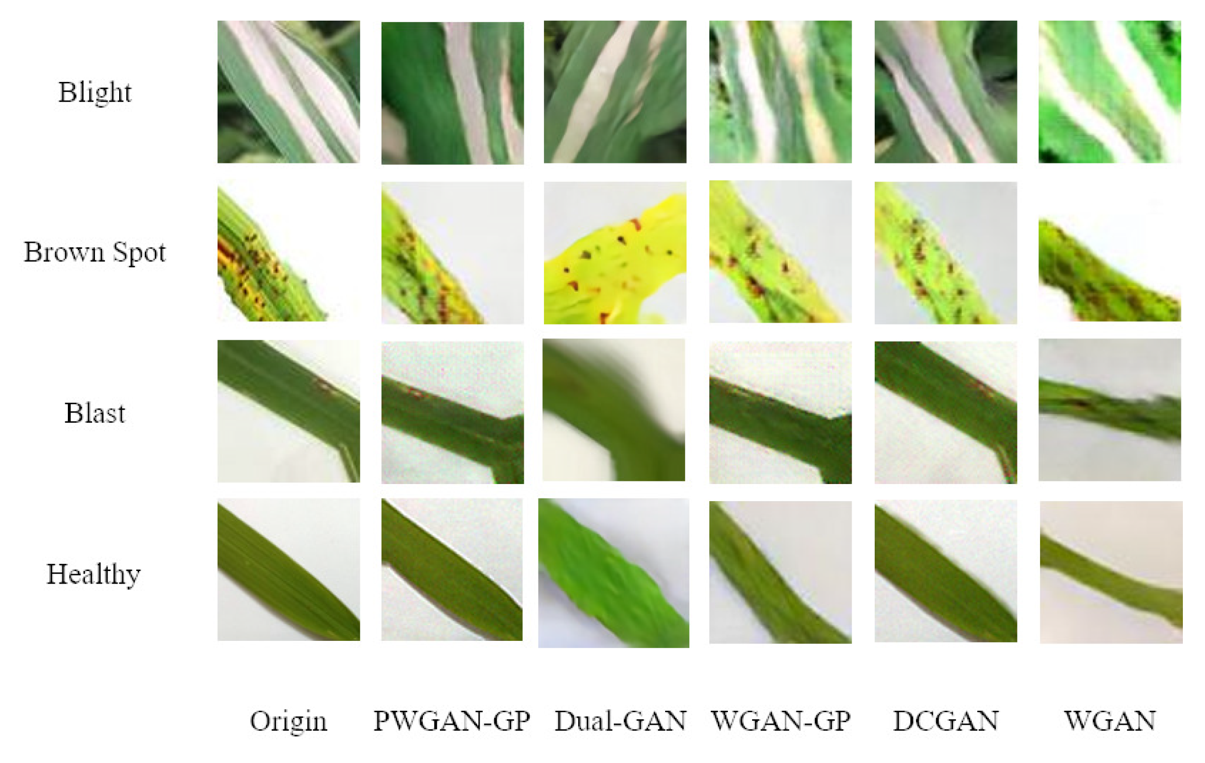
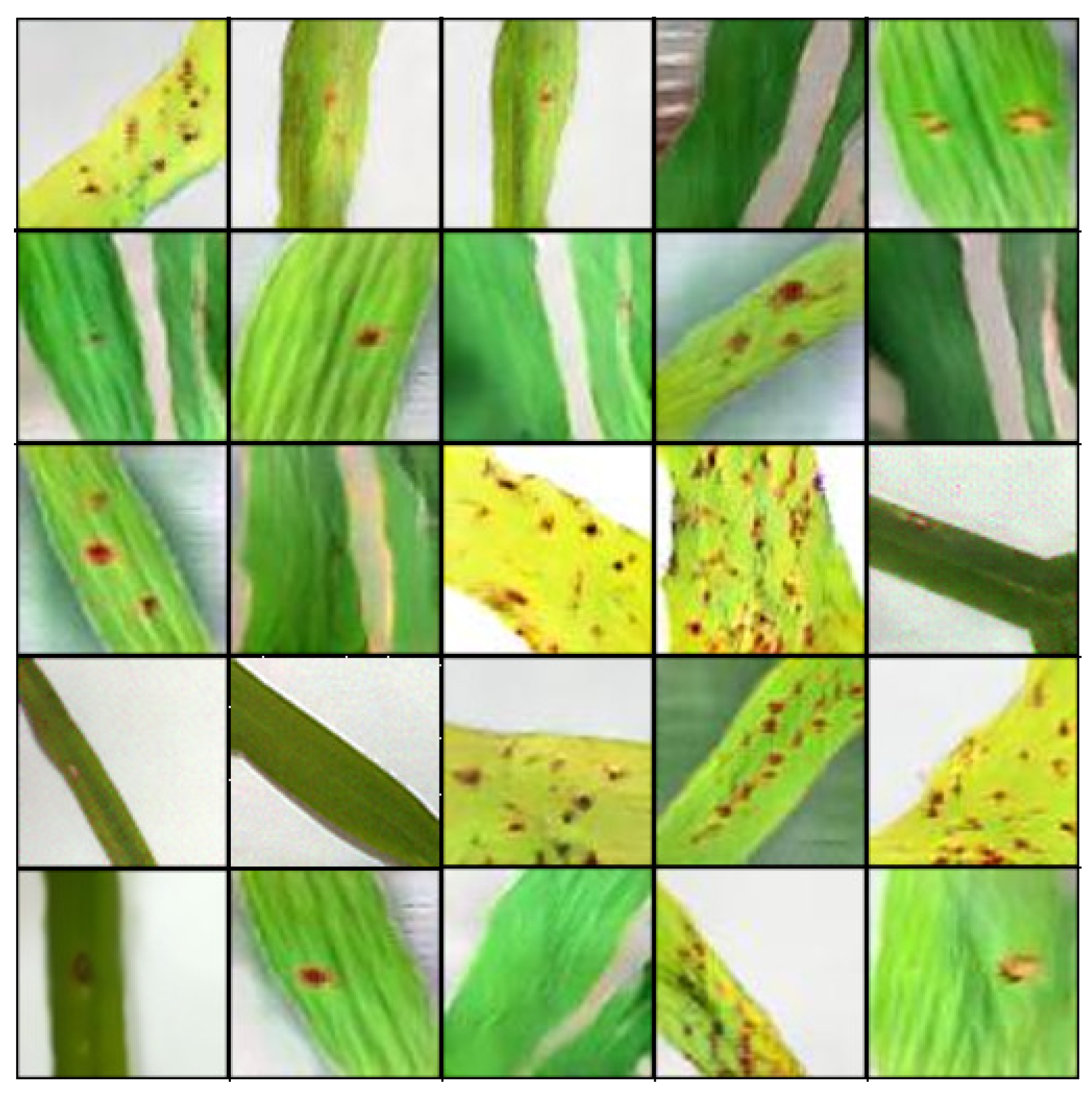
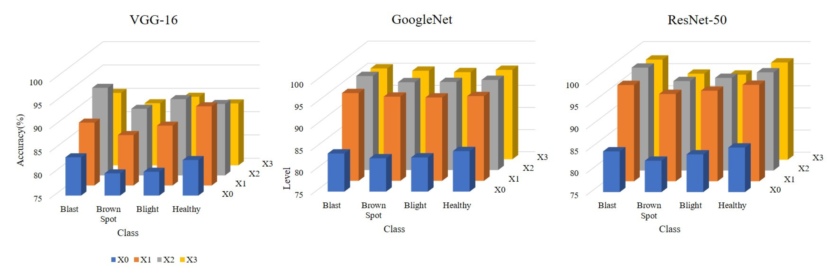
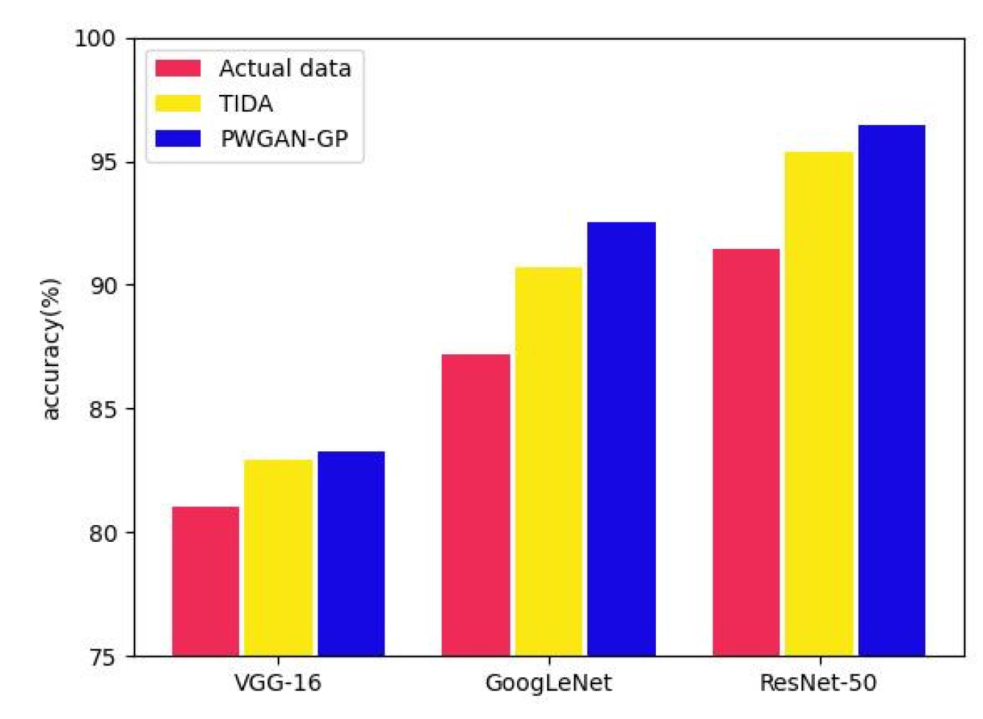
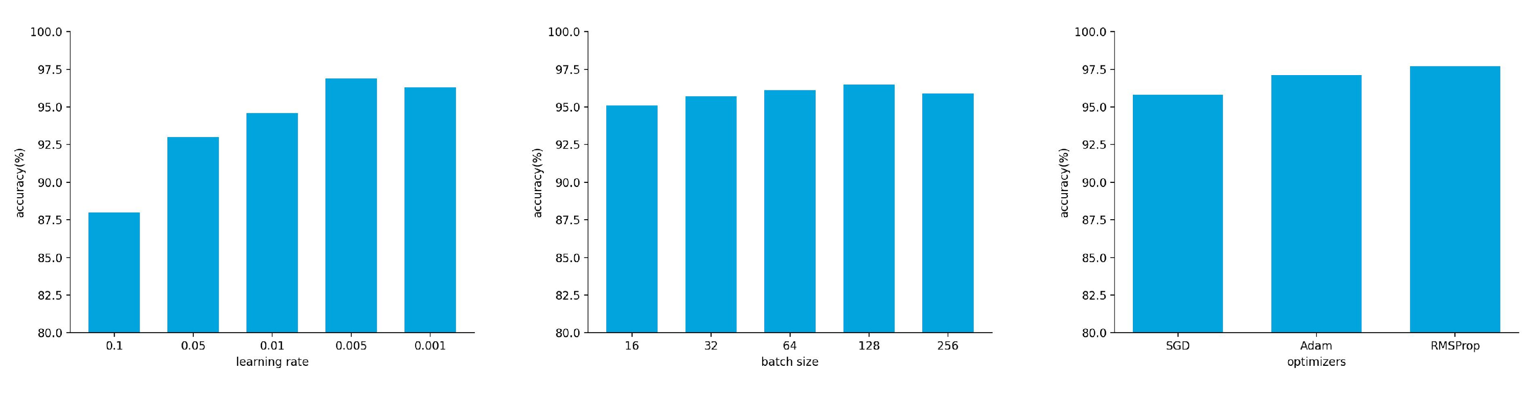
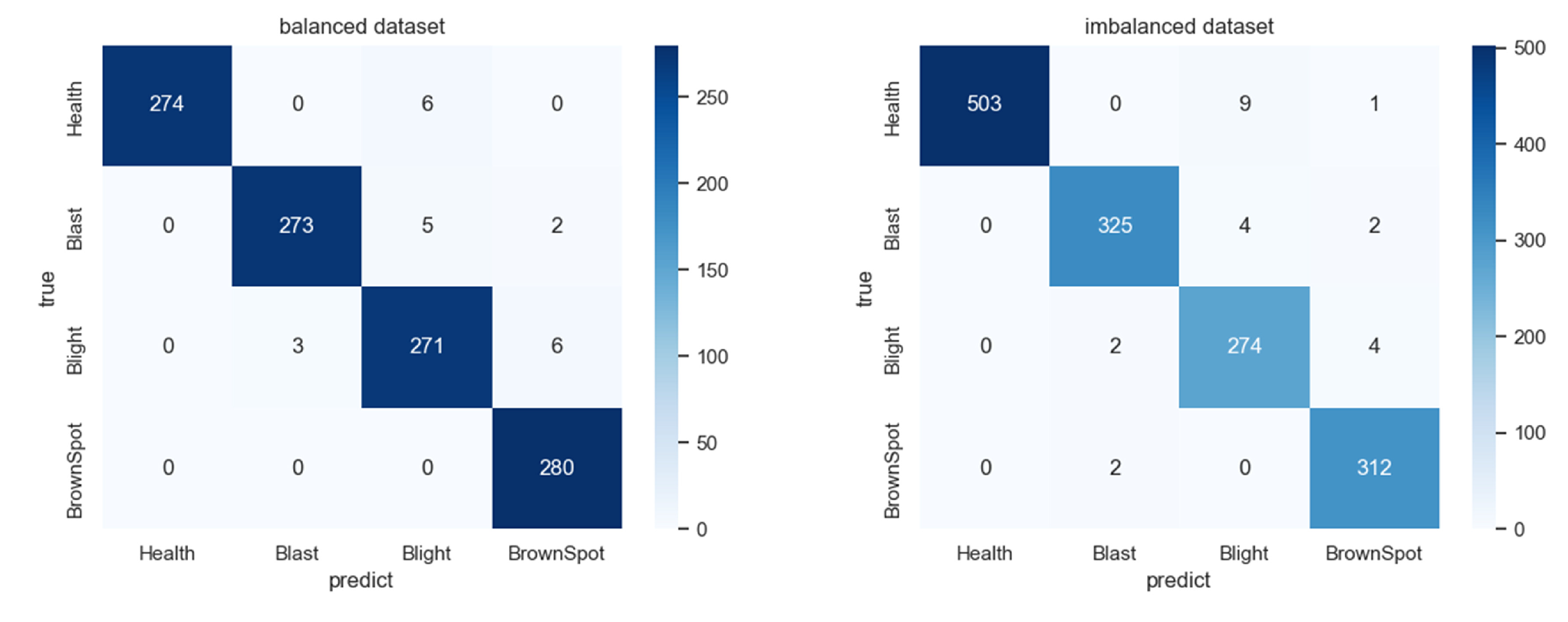
To solve the problem of low accuracy caused by the lack of rice disease image datasets in training CNNs, PWGAN-GP is proposed to generate rice leaf disease images in this paper. First, we use the progressing training method to train the generator model and discriminator model, and a loss function is added to the discriminator model. It has been concluded that the PWGAN-GP network is the best to generate rice leaf disease images compared with WGAN, DCGAN, and WGAN-GP. Second, the experimental results show that the accuracy of VGG-16, GoogLeNet, and ResNet-50 using PWGAN-GP is 10.44%, 12.38%, and 13.19% higher than those without PWGAN-GP. Compared with a traditional image data augmentation method, the accuracy is increased by 3.2%, 3.86%, and 3.11%, respectively. The accuracy of CNNs can be maximized under the condition of X2 (1:20) enhancement intensity. Finally, under hyperparameter optimization, the ResNet-50 with PWGAN-GP achieved 98.14% for identifying three rice diseases. In addition, we also tested the performance of ResNet-50 in some scenarios, and the results were good. Therefore, it has been shown that PWGAN-GP has better image generation ability and improves the classification ability of CNNs.

At present, the model proposed in this paper also has the problem of long training time and slow convergence. In future work, we will solve these two problems by optimizing model parameters and combining deep learning with control theory [48,49,50,51,52].

References

1. Huang, S.; Wang, P.; Yamaji, N.; Ma, J.F. Plant Nutrition for Human Nutrition: Hints from Rice Research and Future Perspectives. Mol. Plant 2020, 13, 825–835. [Google Scholar] [CrossRef]
2. Gayathri Devi, T.; Neelamegam, P. Image processing based rice plant leaves diseases in Thanjavur, Tamilnadu. Clust. Comput. 2019, 22, 13415–13428. [Google Scholar] [CrossRef]
3. Chawathe, S.S. Rice disease detection by image analysis. In Proceedings of the 2020 10th Annual Computing and Communication Workshop and Conference (CCWC), Las Vegas, NV, USA, 6–8 January 2020; pp. 0524–0530. [Google Scholar]
4. Sethy, P.K.; Barpanda, N.K.; Rath, A.K.; Behera, S.K. Deep feature based rice leaf disease identification using support vector machine. Comput. Electron. Agric. 2020, 175, 105527. [Google Scholar] [CrossRef]
5. Sulistyaningrum, D.; Rasyida, A.; Setiyono, B. Rice disease classification based on leaf image using multilevel Support Vector Machine (SVM). J. Phys. Conf. Ser. 2020, 1490, 012053. [Google Scholar] [CrossRef]
6. Adiyarta, K.; Zonyfar, C.; Fatimah, T. Identification of rice leaf disease based on rice leaf image features using the k-Nearest Neighbour (k-NN) technique. In Proceedings of the International Conference on IT, Communication and Technology for Better Life, ICT4BL, Bangkok, Thailand, 17–18 July 2019; pp. 160–165. [Google Scholar]
7. Mekha, P.; Teeyasuksaet, N. Image Classification of Rice Leaf Diseases Using Random Forest Algorithm. In Proceedings of the 2021 Joint International Conference on Digital Arts, Media and Technology with ECTI Northern Section Conference on Electrical, Electronics, Computer and Telecommunication Engineering, Cha-am, Thailand, 3–6 March 2021; pp. 165–169. [Google Scholar]
8. Rasjava, A.R.; Sugiyarto, A.W.; Kurniasari, Y.; Ramadhan, S.Y. Detection of Rice Plants Diseases Using Convolutional Neural Network (CNN). In Proceedings of the International Conference on Science and Engineering, Male, Maldives, 14–16 January 2020; Volume 3, pp. 393–396. [Google Scholar]
9. Zhang, X.; Qiao, Y.; Meng, F.; Fan, C.; Zhang, M. Identification of maize leaf diseases using improved deep convolutional neural networks. IEEE Access 2018, 6, 30370–30377. [Google Scholar] [CrossRef]
10. Swasono, D.I.; Tjandrasa, H.; Fathicah, C. Classification of tobacco leaf pests using VGG16 transfer learning. In Proceedings of the 2019 12th International Conference on Information & Communication Technology and System (ICTS), Surabaya, Indonesia, 18 July 2019; pp. 176–181. [Google Scholar]
11. LeCun, Y.; Bengio, Y.; Hinton, G. Deep learning. Nature 2015, 521, 436–444. [Google Scholar] [CrossRef] [PubMed]
12. Kc, K.; Yin, Z.; Wu, M.; Wu, Z. Depthwise Separable Convolution Architectures for Plant Disease Classification. Comput. Electron. Agric. 2019, 165, 104948. [Google Scholar] [CrossRef]
13. Hossain, S.M.M.; Deb, K.; Dhar, P.K.; Koshiba, T. Plant Leaf Disease Recognition Using Depth-Wise Separable Convolution-Based Models. Symmetry 2021, 13, 511. [Google Scholar] [CrossRef]
14. Yakkundimath, R.; Saunshi, G.; Anami, B.; Palaiah, S. Classification of Rice Diseases Using Convolutional Neural Network Models. J. Inst. Eng. (India) Ser. B 2022, 103, 1047–1059. [Google Scholar] [CrossRef]
15. Liang, W.j.; Zhang, H.; Zhang, G.f.; Cao, H.x. Rice blast disease recognition using a deep convolutional neural network. Sci. Rep. 2019, 9, 1–10. [Google Scholar] [CrossRef] [Green Version]
16. Belkin, M.; Ma, S.; Mandal, S. To understand deep learning we need to understand kernel learning. In Proceedings of the International Conference on Machine Learning, PMLR, Stockholm, Sweden, 10–15 July 2018; pp. 541–549. [Google Scholar]
17. D’souza, R.N.; Huang, P.Y.; Yeh, F.C. Structural analysis and optimization of convolutional neural networks with a small sample size. Sci. Rep. 2020, 10, 834. [Google Scholar] [CrossRef] [Green Version]
18. Johnson, J.M.; Khoshgoftaar, T.M. Survey on deep learning with class imbalance. J. Big Data 2019, 6, 1–54. [Google Scholar] [CrossRef] [Green Version]
19. Zhang, R. Making Convolutional Networks Shift-Invariant Again. arXiv 2019. [Google Scholar] [CrossRef]
20. Goodfellow, I.J.; Pouget-Abadie, J.; Mirza, M.; Xu, B.; Warde-Farley, D.; Ozair, S.; Courville, A.; Bengio, Y. Generative adversarial nets. Adv. Neural Inf. Process. Syst. 2014, 27, 1–9. [Google Scholar]
21. Arjovsky, M.; Chintala, S.; Bottou, L. Wasserstein Generative Adversarial Networks. In Proceedings of the International Conference on Machine Learning, Sydney, Australia, 6–11 August 2017. [Google Scholar]
22. Gulrajani, I.; Ahmed, F.; Arjovsky, M.; Dumoulin, V.; Courville, A.C. Improved Training of Wasserstein GANs. In Proceedings of the Advances in Neural Information Processing Systems 30 (NIPS 2017), Long Beach, CA, USA, 4–9 December 2017; Volume 30. [Google Scholar]
23. Abbas, A.; Jain, S.; Gour, M.; Vankudothu, S. Tomato plant disease detection using transfer learning with C-GAN synthetic images. Comput. Electron. Agric. 2021, 187, 106279. [Google Scholar] [CrossRef]
24. Bing, L.; Yong, X.; Daqiao, Z. Infrared Image Generation Algorithm Based on Conditional Generation Adversarial Networks. Acta Photonica Sin. 2021, 50, 1110004. [Google Scholar]
25. Nazki, H.; Lee, J.; Yoon, S.; Park, D.S. Image-to-image translation with GAN for synthetic data augmentation in plant disease datasets. Smart Media J. 2019, 8, 46–57. [Google Scholar] [CrossRef]
26. Yang, Q.; Lu, J.G.; Tang, X.H.; Gu, X.; Sheng, X.J.; Yang, R.H. Bearing small sample fault diagnosis based on InfoGAN and CNN. J. Ordnance Equip. Eng. 2021, 42, 235–240. [Google Scholar]
27. Liu, Y.; Zhou, Y.; Liu, X.; Dong, F.; Wang, C.; Wang, Z. Wasserstein GAN-based small-sample augmentation for new-generation artificial intelligence: A case study of cancer-staging data in biology. Engineering 2019, 5, 156–163. [Google Scholar] [CrossRef]
28. Sandfort, V.; Yan, K.; Pickhardt, P.J.; Summers, R.M. Data augmentation using generative adversarial networks (CycleGAN) to improve generalizability in CT segmentation tasks. Sci. Rep. 2019, 9, 16884. [Google Scholar] [CrossRef] [Green Version]
29. Karras, T.; Aila, T.; Laine, S.; Lehtinen, J. Progressive growing of gans for improved quality, stability, and variation. arXiv 2017, arXiv:1710.10196. [Google Scholar]
30. Zhang, Z.; Gao, Q.; Liu, L.; He, Y. A High-Quality Rice Leaf Disease Image Data Augmentation Method Based on a Dual GAN. IEEE Access 2023, 11, 21176–21191. [Google Scholar] [CrossRef]
31. Lamba, S.; Baliyan, A.; Kukreja, V. A Novel GCL Hybrid Classification Model for Paddy Diseases. Int. J. Inf. Technol. 2023, 15, 1127–1136. [Google Scholar] [CrossRef] [PubMed]
32. Lamba, S.; Baliyan, A.; Kukreja, V. GAN Based Image Augmentation for Increased CNN Performance in Paddy Leaf Disease Classification. In Proceedings of the 2022 2nd International Conference on Advance Computing and Innovative Technologies in Engineering (ICACITE), Greater Noida, India, 28–29 April 2022; pp. 2054–2059. [Google Scholar] [CrossRef]
33. Shayan, R. Rice Leafs. 2019. Available online: https://www.kaggle.com/shayanriyaz/riceleafs (accessed on 24 February 2023).
34. Marsh. Rice Leaf Diseases Dataset. 2019. Available online: https://www.kaggle.com/vbookshelf/rice-leaf-diseases (accessed on 24 February 2023).
35. Rajeshbhattacharjee. rice_diseases_using_cnn_and_svm. 2019. Available online: https://www.kaggle.com/rajeshbhattacharjee/rice-diseases-using-cnn-and-svm (accessed on 24 February 2023).
36. He, K.; Zhang, X.; Ren, S.; Sun, J. Deep residual learning for image recognition. In Proceedings of the IEEE Conference on Computer Vision and Pattern Recognition, Las Vegas, NV, USA, 27–30 June 2016; pp. 770–778. [Google Scholar]
37. Ding, W.; Taylor, G. Automatic moth detection from trap images for pest management. Comput. Electron. Agric. 2016, 123, 17–28. [Google Scholar] [CrossRef] [Green Version]
38. Dumoulin, V.; Visin, F. A guide to convolution arithmetic for deep learning. arXiv 2016, arXiv:1603.07285. [Google Scholar]
39. Ioffe, S.; Szegedy, C. Batch normalization: Accelerating deep network training by reducing internal covariate shift. In Proceedings of the International Conference on Machine Learning, Lille, France, 6–11 July 2015; pp. 448–456. [Google Scholar]
40. Ioffe, S.; Normalization, C.S.B. Accelerating deep network training by reducing internal covariate shift. arXiv 2014, arXiv:1502.03167. [Google Scholar]
41. Wang, S.H.; Muhammad, K.; Hong, J.; Sangaiah, A.K.; Zhang, Y.D. Alcoholism Identification via Convolutional Neural Network Based on Parametric ReLU, Dropout, and Batch Normalization. Neural Comput. Appl. 2020, 32, 665–680. [Google Scholar] [CrossRef]
42. Azulay, A.; Weiss, Y. Why Do Deep Convolutional Networks Generalize so Poorly to Small Image Transformations? arXiv 2019, arXiv:1805.12177. [Google Scholar]
43. Heusel, M.; Ramsauer, H.; Unterthiner, T.; Nessler, B.; Hochreiter, S. Gans trained by a two time-scale update rule converge to a local nash equilibrium. In Proceedings of the Advances in Neural Information Processing Systems 30 (NIPS 2017), Long Beach, CA, USA, 4–9 December 2017; Volume 30. [Google Scholar]
44. Jiang, F.; Lu, Y.; Chen, Y.; Cai, D.; Li, G. Image recognition of four rice leaf diseases based on deep learning and support vector machine. Comput. Electron. Agric. 2020, 179, 105824. [Google Scholar] [CrossRef]
45. Jadhav, S.B.; Udupi, V.R.; Patil, S.B. Identification of plant diseases using convolutional neural networks. Int. J. Inf. Technol. 2021, 13, 2461–2470. [Google Scholar] [CrossRef]
46. Sethy, P.K.; Barpanda, N.K.; Rath, A.K.; Behera, S.K. Nitrogen deficiency prediction of rice crop based on convolutional neural network. J. Ambient. Intell. Humaniz. Comput. 2020, 11, 5703–5711. [Google Scholar] [CrossRef]
47. Hossain, S.M.M.; Tanjil, M.M.M.; Ali, M.A.B.; Islam, M.Z.; Islam, M.S.; Mobassirin, S.; Sarker, I.H.; Islam, S.M.R. Rice Leaf Diseases Recognition Using Convolutional Neural Networks. In Proceedings of the Advanced Data Mining and Applications, Foshan, China, 12–14 November 2020; Yang, X., Wang, C.D., Islam, M.S., Zhang, Z., Eds.; Lecture Notes in Computer Science. Springer: Cham, Switzerland; pp. 299–314. [Google Scholar] [CrossRef]
48. Hu, J.; Jia, C.; Liu, H.; Yi, X.; Liu, Y. A survey on state estimation of complex dynamical networks. Int. J. Syst. Sci. 2021, 52, 3351–3367. [Google Scholar] [CrossRef]
49. Hu, J.; Zhang, H.; Liu, H.; Yu, X. A survey on sliding mode control for networked control systems. Int. J. Syst. Sci. 2021, 52, 1129–1147. [Google Scholar] [CrossRef]
50. Tan, H.; Shen, B.; Peng, K.; Liu, H. Robust recursive filtering for uncertain stochastic systems with amplify-and-forward relays. Int. J. Syst. Sci. 2020, 51, 1188–1199. [Google Scholar] [CrossRef]
51. Li, X.; Han, F.; Hou, N.; Dong, H.; Liu, H. Set-membership filtering for piecewise linear systems with censored measurements under Round-Robin protocol. Int. J. Syst. Sci. 2020, 51, 1578–1588. [Google Scholar] [CrossRef]
52. Li, Q.; Liang, J. Dissipativity of the stochastic Markovian switching CVNNs with randomly occurring uncertainties and general uncertain transition rates. Int. J. Syst. Sci. 2020, 51, 1102–1118. [Google Scholar] [CrossRef]
Figure 1. Images of rice diseases collected.
Remotesensing 15 01789 g001
Figure 2. Dataset split strategy.
Remotesensing 15 01789 g002
Figure 3. Weight clipping.
Remotesensing 15 01789 g003
Figure 4. Gradient penalty.
Remotesensing 15 01789 g004
Figure 5. Residual block.
Remotesensing 15 01789 g005
Figure 6. PWGAN-GP model.
Remotesensing 15 01789 g006
Figure 7. New layer fusion.
Remotesensing 15 01789 g007
Figure 8. Two-layer residual block.
Remotesensing 15 01789 g008
Figure 9. TIDA approach, where (a) is the original image, (b) rotation, (c) panning, (d) scaling, (e) brightness adjustment, (f) contrast adjustment, and (g) adding noise.
Remotesensing 15 01789 g009
Figure 10. Flow chart of the experimental framework.
Remotesensing 15 01789 g010
Figure 11. Comparison of generated samples.
Remotesensing 15 01789 g011
Figure 12. The images generated by PWGAN-GP.
Remotesensing 15 01789 g012
Figure 13. Effect of reducing the number of training sets on PWGAN-GP.
Remotesensing 15 01789 g013
Figure 14. The effect of the level of data enhancement on the accuracy of neural network models.
Remotesensing 15 01789 g014
Figure 15. Impact of data enhancement on the accuracy of neural networks.
Remotesensing 15 01789 g015
Figure 16. Hyperparameter optimization of ResNet-50.
Remotesensing 15 01789 g016
Figure 17. ResNet-50 training chart under optimal hyperparameter.
Remotesensing 15 01789 g017
Figure 18. Confusion matrix for the effect of imbalanced test set on ResNet-50 test results.
Remotesensing 15 01789 g018
Figure 19. Datasets in complex environments.
Remotesensing 15 01789 g019
Figure 20. ResNet-50 forward propagation feature map.
Remotesensing 15 01789 g020