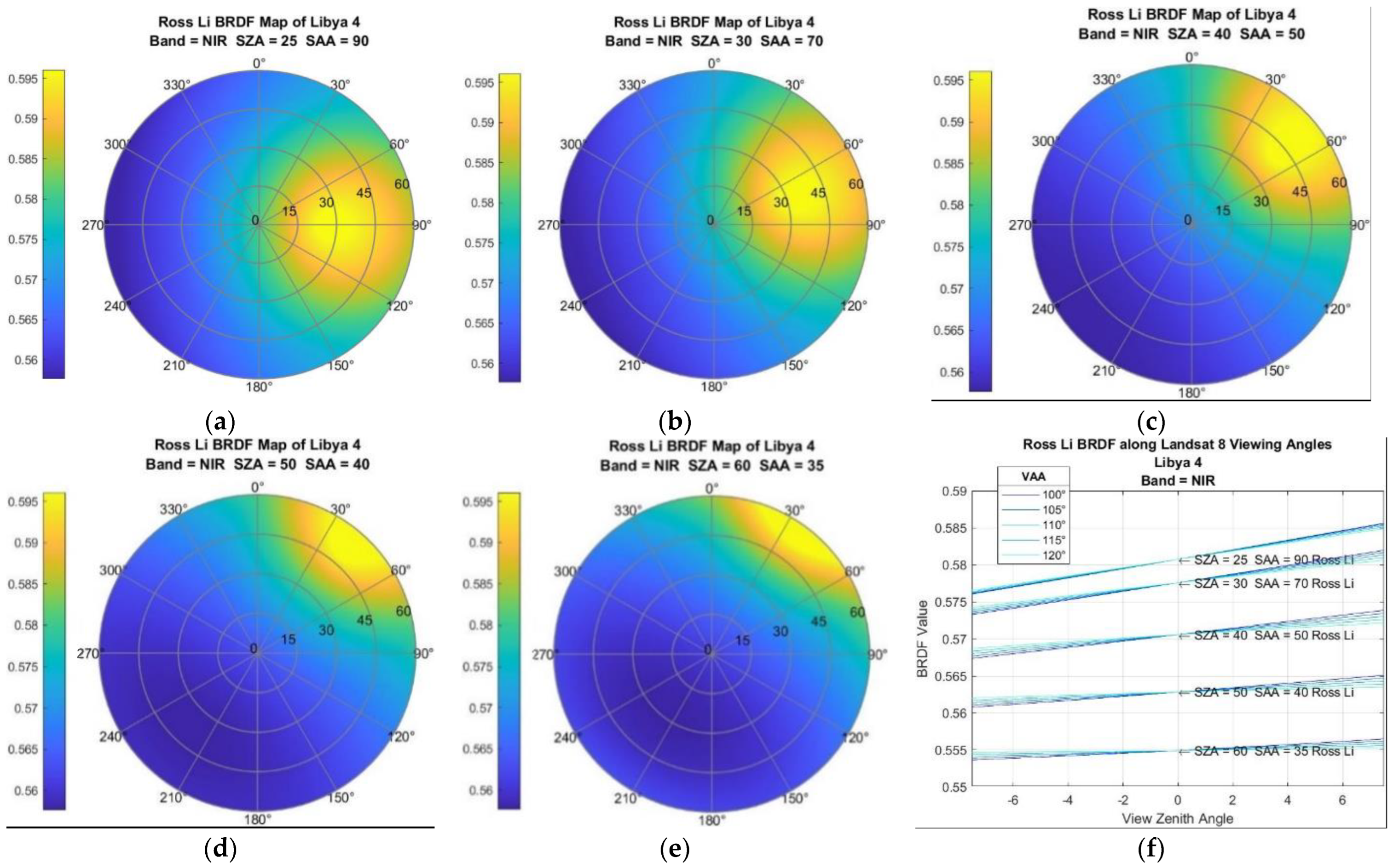
Figure 1.
(
a–
e): BRDF models of grass pasture for different SZA and SAA locations. Note how hot spot follows solar location as the sun moves lower in the sky. (
f): Linearity of BRDF versus VZA for entire range of Landsat viewing angles. Note how the slope is greater as the sensor view angle moves closer to the “hot spot”. Image source: [
5].
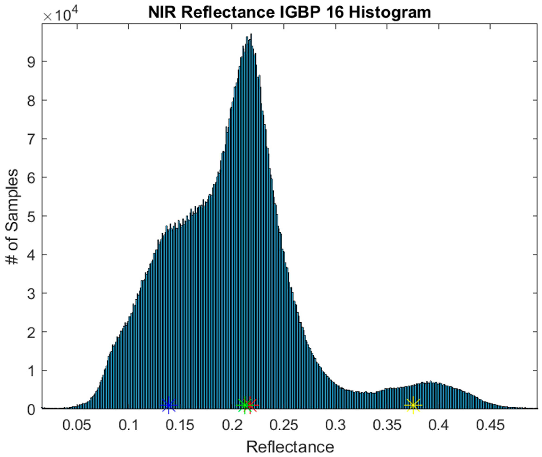
Figure 2.
Global NIR reflectance distribution of barren land cover. Note that the colored stars are the reflectance values for each group calculated by the k-means algorithm.
Figure 2.
Global NIR reflectance distribution of barren land cover. Note that the colored stars are the reflectance values for each group calculated by the k-means algorithm.
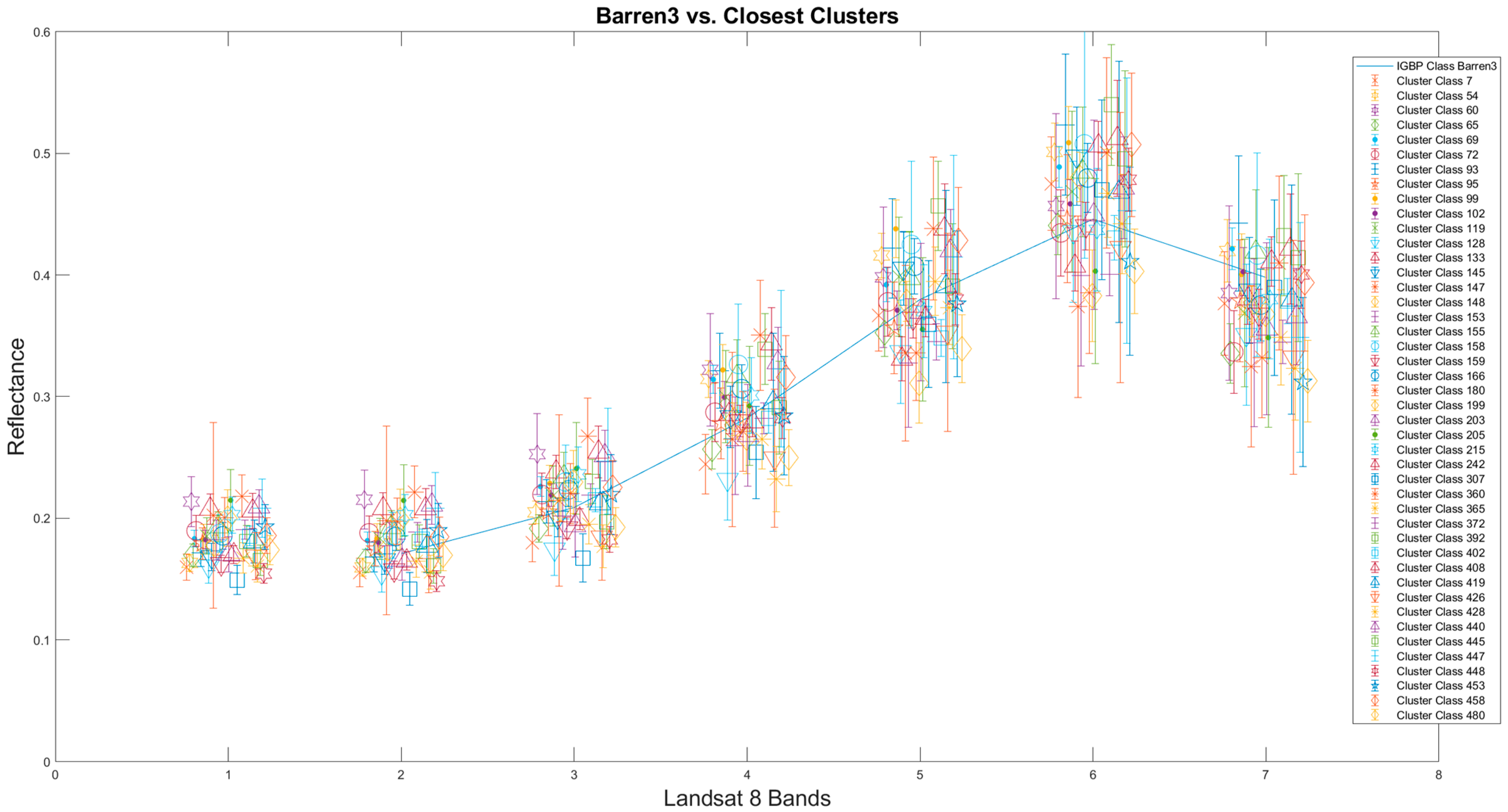
Figure 3.
Barren3 reflectance profile plotted against matching clusters. Note the clusters grouping around the banded IGBP profile. The CA band does not have an IGBP value since MODIS does not have a CA band equivalent.
Figure 3.
Barren3 reflectance profile plotted against matching clusters. Note the clusters grouping around the banded IGBP profile. The CA band does not have an IGBP value since MODIS does not have a CA band equivalent.
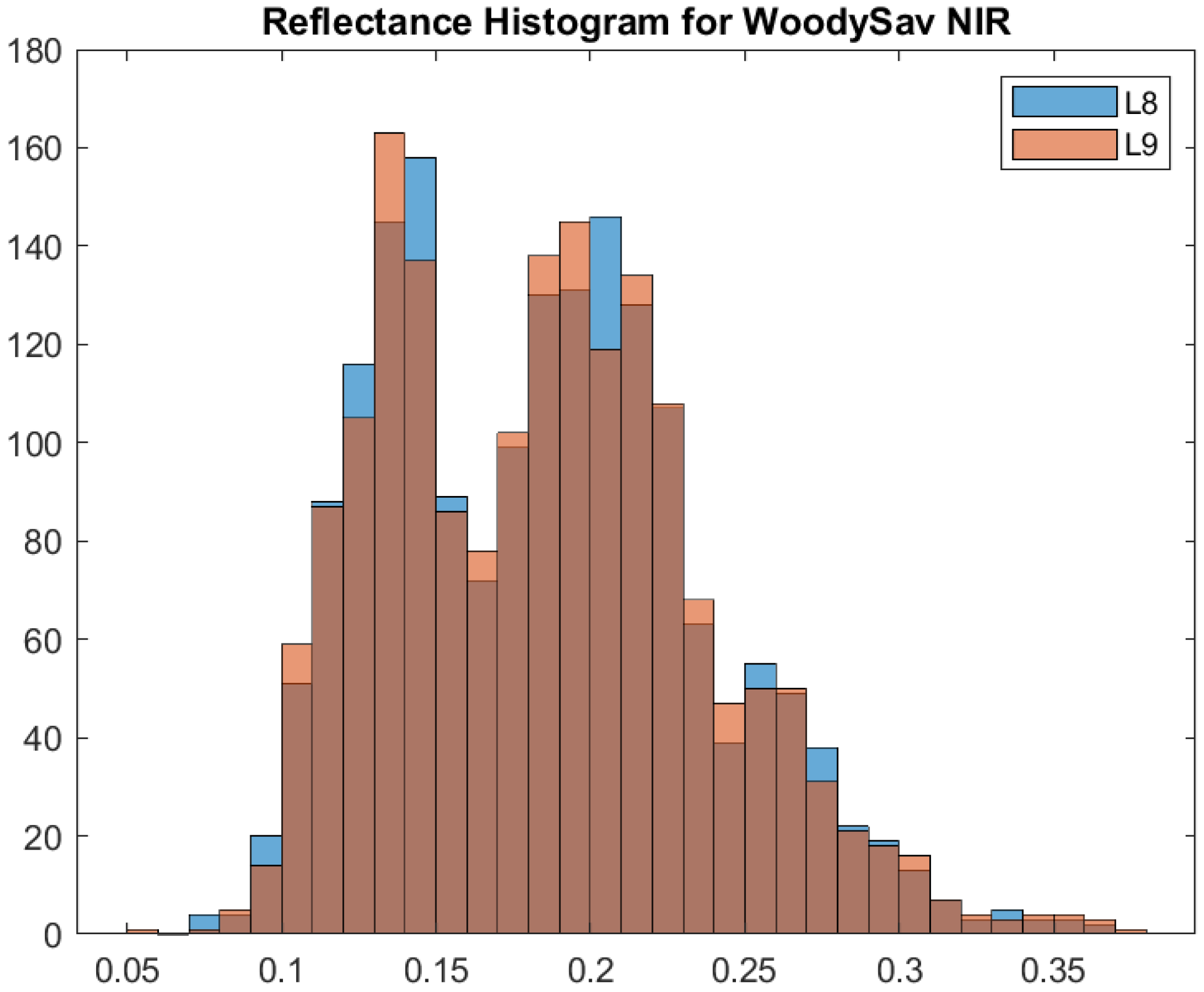
Figure 4.
Woody Savanna IGBP global NIR band reflectance distribution. Note the two peaks in the distribution.
Figure 4.
Woody Savanna IGBP global NIR band reflectance distribution. Note the two peaks in the distribution.
Figure 5.
(a) Woody Savanna global NIR band reflectance distribution. This plot corresponds to reflectances above the Tropic of Cancer latitude. (b) This plot corresponds to reflectances below Tropic of Cancer. Note the peaks split up after separating by latitude.
Figure 5.
(a) Woody Savanna global NIR band reflectance distribution. This plot corresponds to reflectances above the Tropic of Cancer latitude. (b) This plot corresponds to reflectances below Tropic of Cancer. Note the peaks split up after separating by latitude.
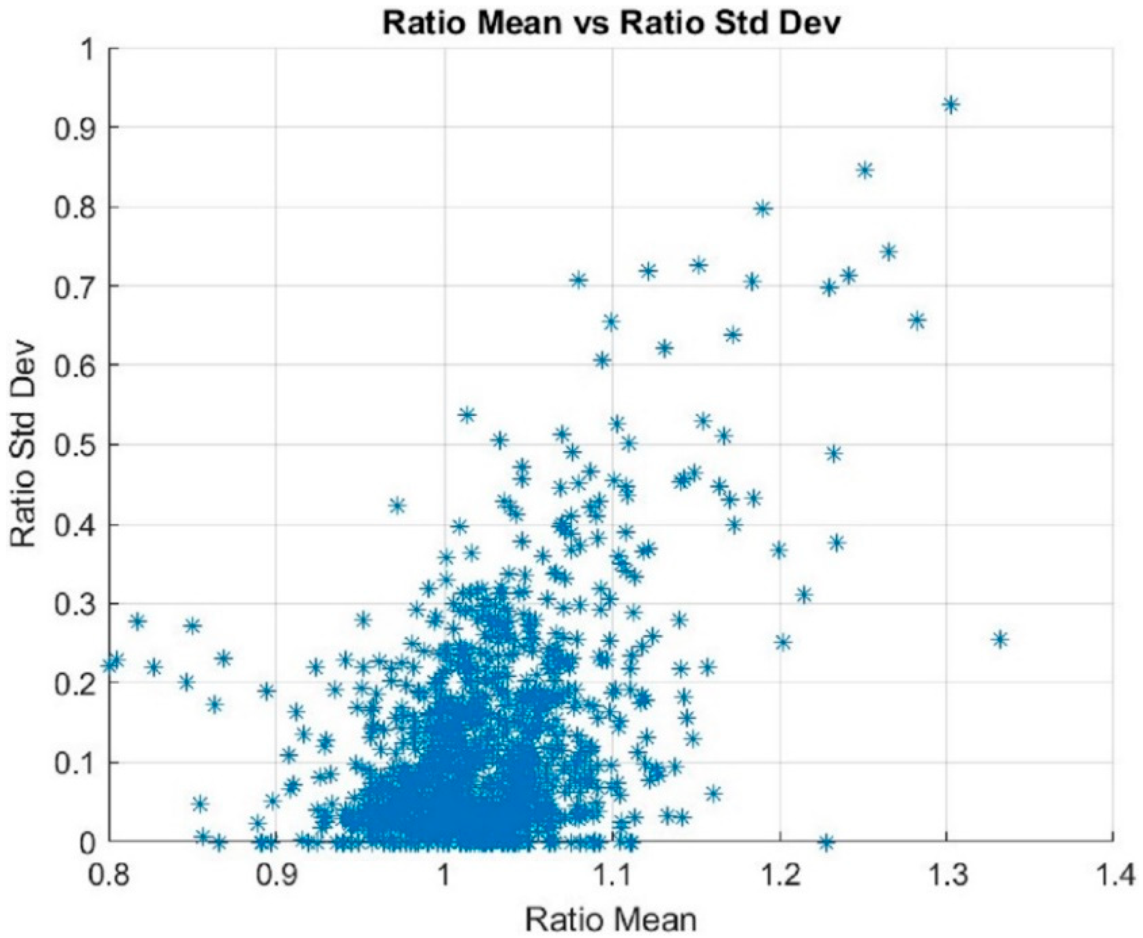
Figure 6.
Ratio mean vs. ratio standard deviation. Note the discernable positive linear trend above a ratio standard deviation of 0.2 as the data drift to larger values. Since the ratio is derived by taking the reflectance of Landsat 8 to 9, this behavior could be a real and observable phenomenon. Image source: [
5].
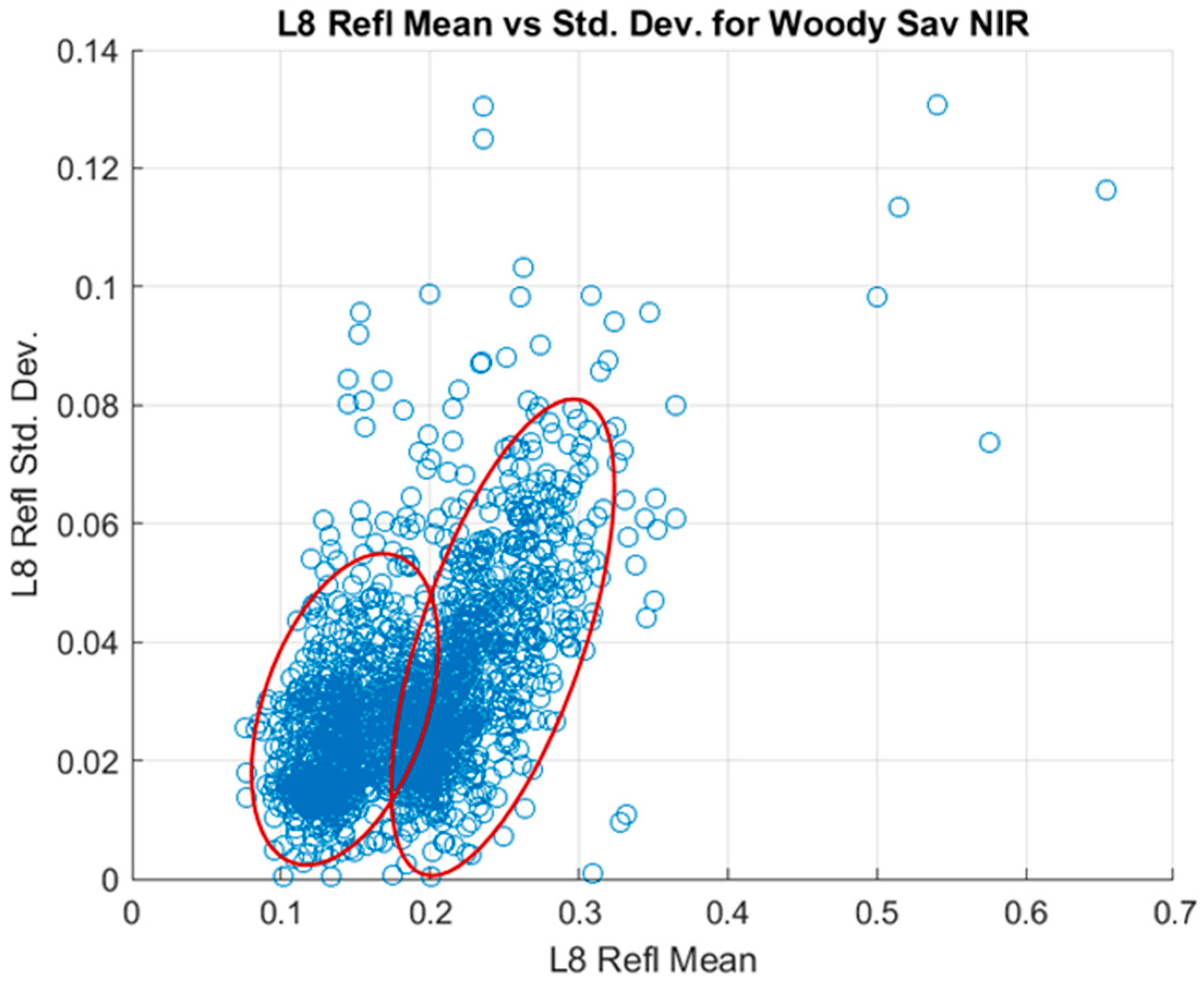
Figure 7.
Signal to noise relationship of Woody Savanna NIR band. Note the two clusters of data points, which can be discerned by latitude.
Figure 7.
Signal to noise relationship of Woody Savanna NIR band. Note the two clusters of data points, which can be discerned by latitude.
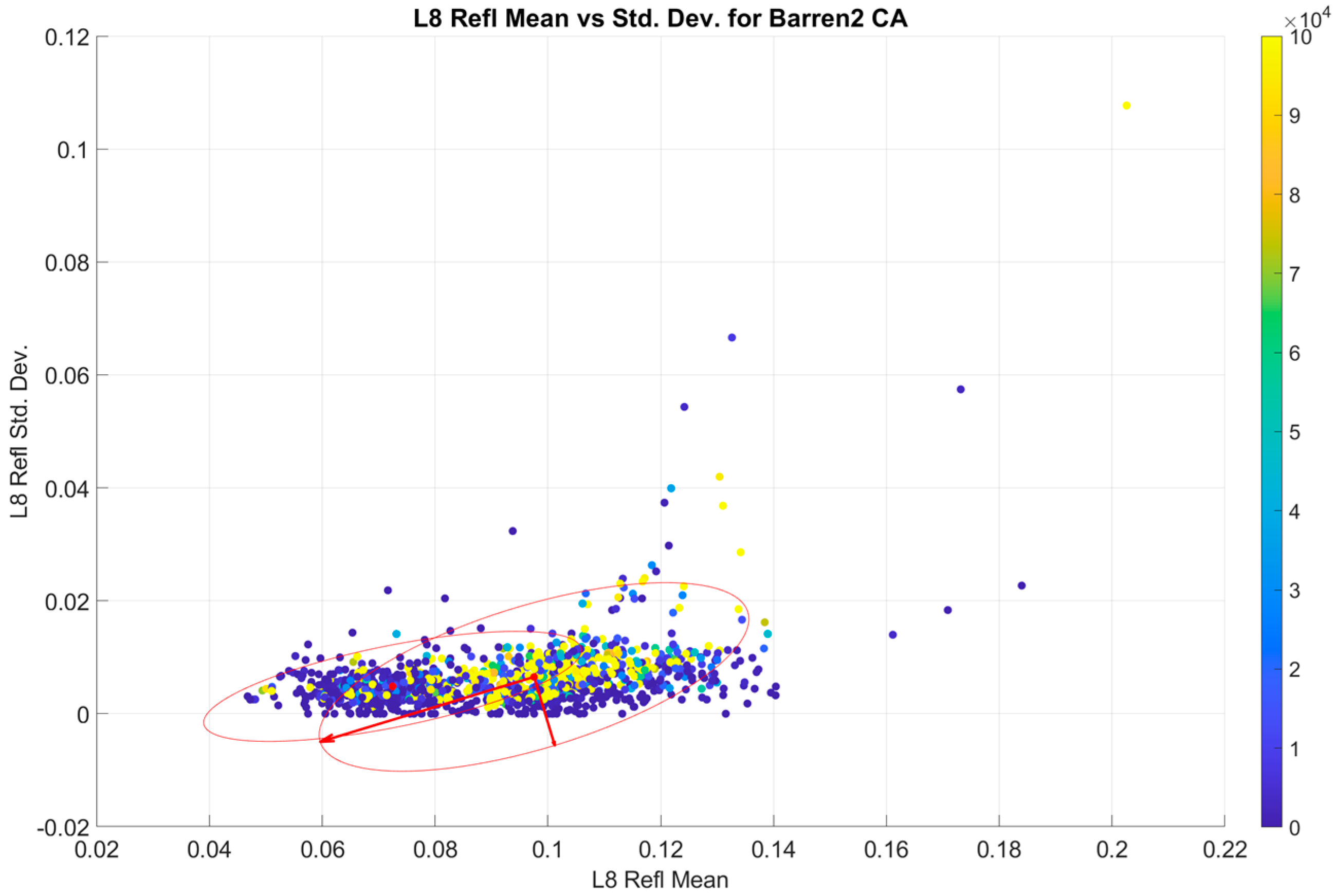
Figure 8.
Weighted ellipse filter for Barren2 CA band, with the eigenvectors dictating the shape of the ellipse. Note that in this example, the high pixel counts of the outliers “pull” the slope of the ellipse up. The points are color coded by pixel count, with the scale on the right of the plot. The arrows indicate the eigenvectors that create the boundaries of the ellipse.
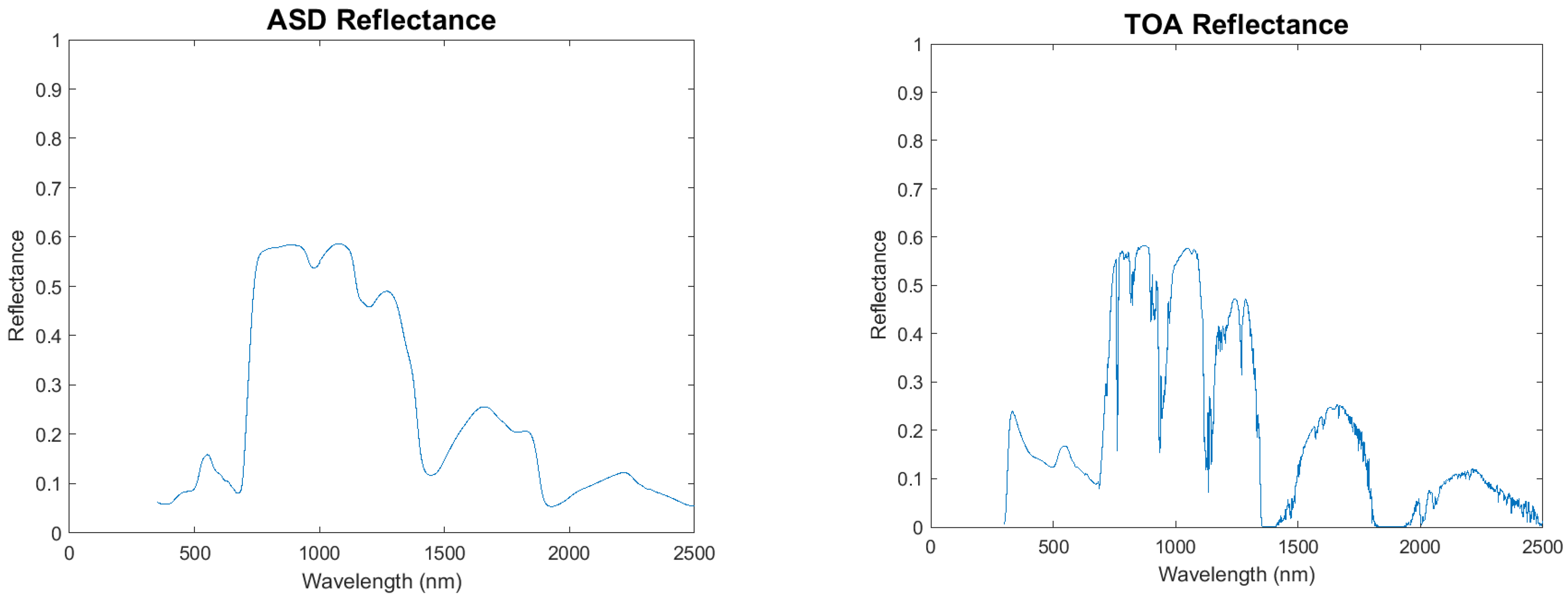
Figure 9.
Surface level reflectance of a white fir tree vs. MODTRAN-simulated TOA reflectance. Note the water absorption in the longer wavelengths and the scattering due to aerosols in the shorter wavelengths.
Figure 9.
Surface level reflectance of a white fir tree vs. MODTRAN-simulated TOA reflectance. Note the water absorption in the longer wavelengths and the scattering due to aerosols in the shorter wavelengths.
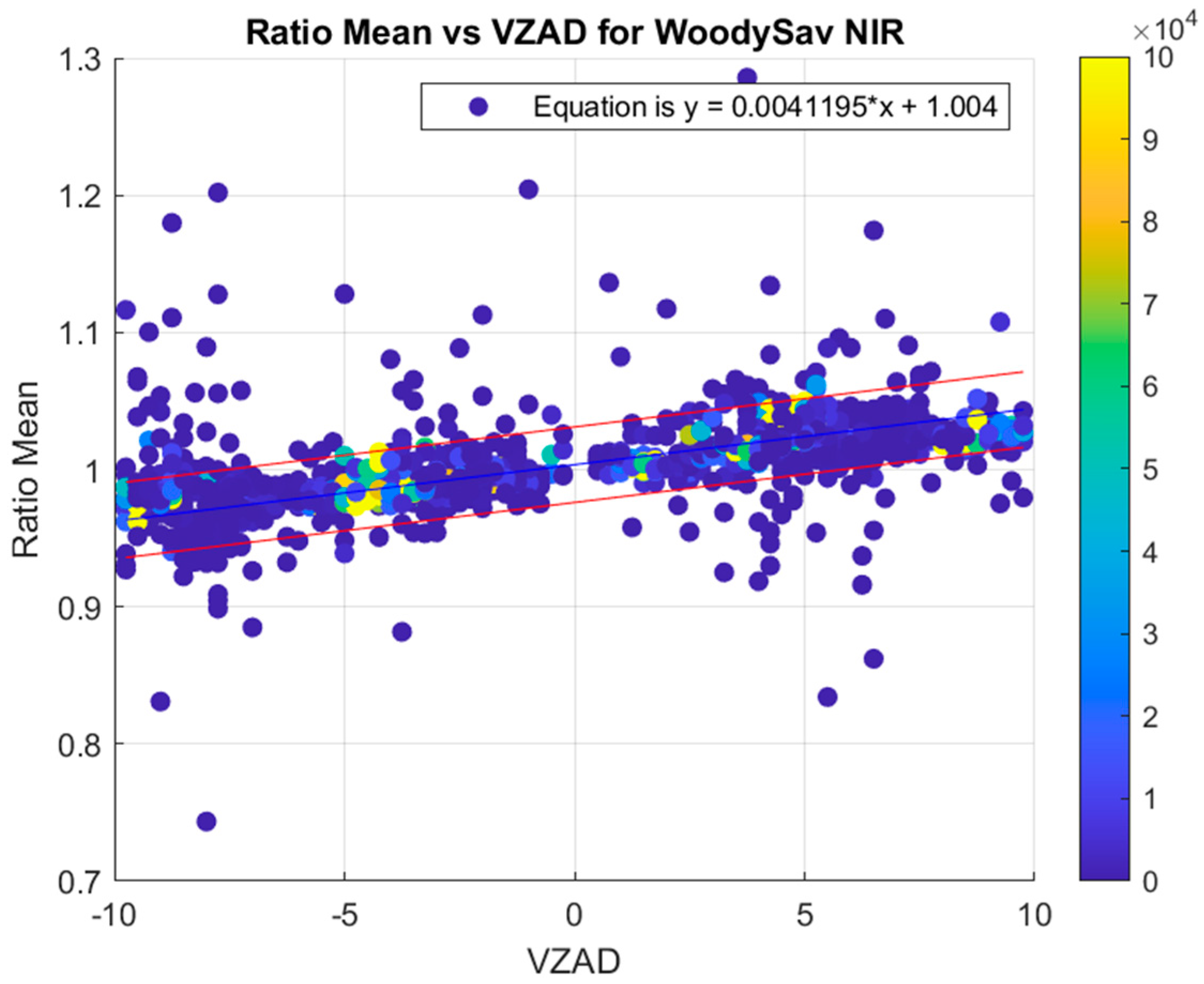
Figure 10.
VZAD vs. ratio mean weighted linear fit. Note the colored data points which indicate the number of pixels per observation, with yellow points being weighted higher in the linear fit equation.
Figure 10.
VZAD vs. ratio mean weighted linear fit. Note the colored data points which indicate the number of pixels per observation, with yellow points being weighted higher in the linear fit equation.
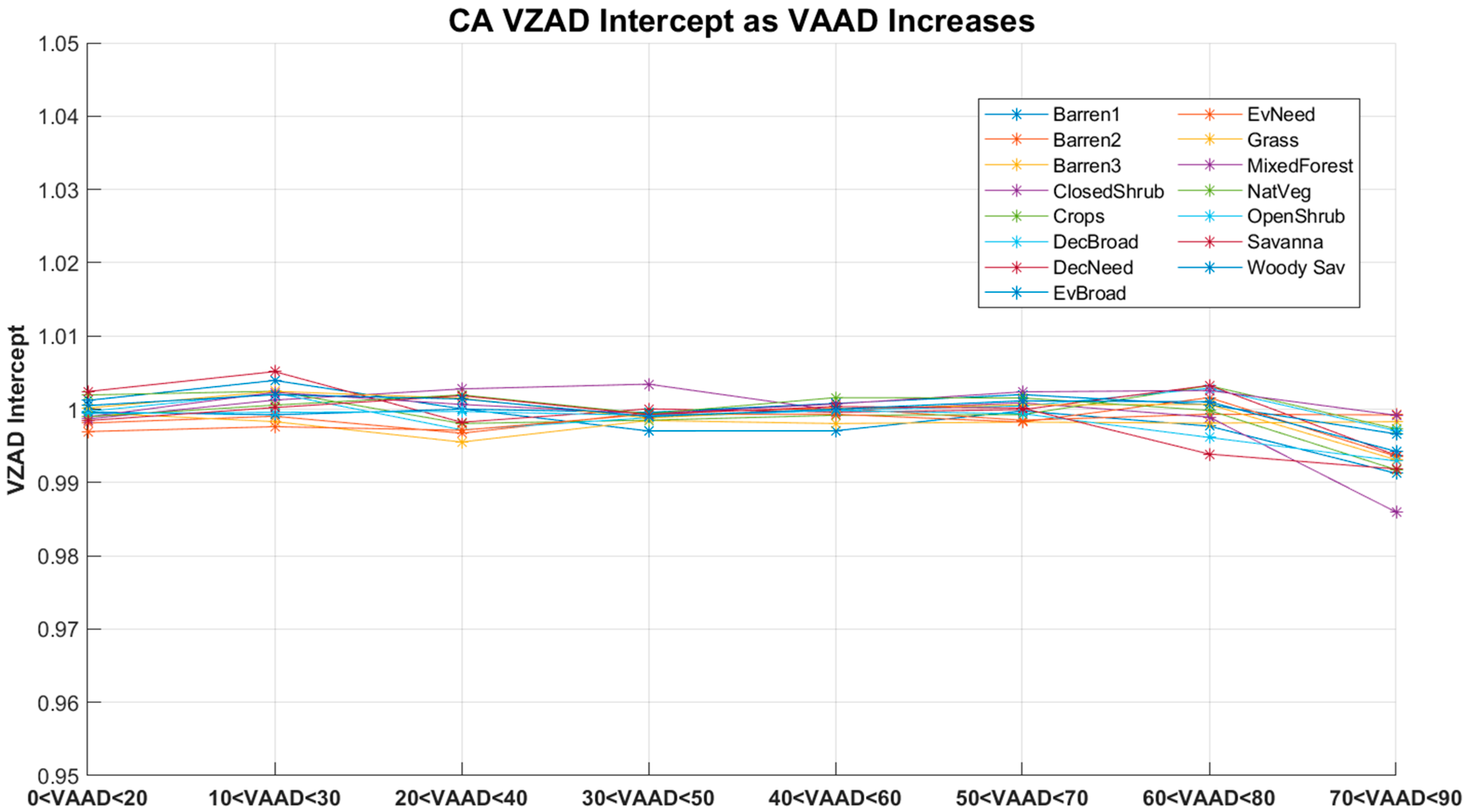
Figure 11.
The VZAD intercept for all IGBP types as VAAD increases from 0–90° in the CA band. Note how the intercepts are about ±0.5% for all VZAD slices, except at the 70 < VAAD < 90 range, which is likely driven by number of samples; there are very few underfly scenes at that range.
Figure 11.
The VZAD intercept for all IGBP types as VAAD increases from 0–90° in the CA band. Note how the intercepts are about ±0.5% for all VZAD slices, except at the 70 < VAAD < 90 range, which is likely driven by number of samples; there are very few underfly scenes at that range.
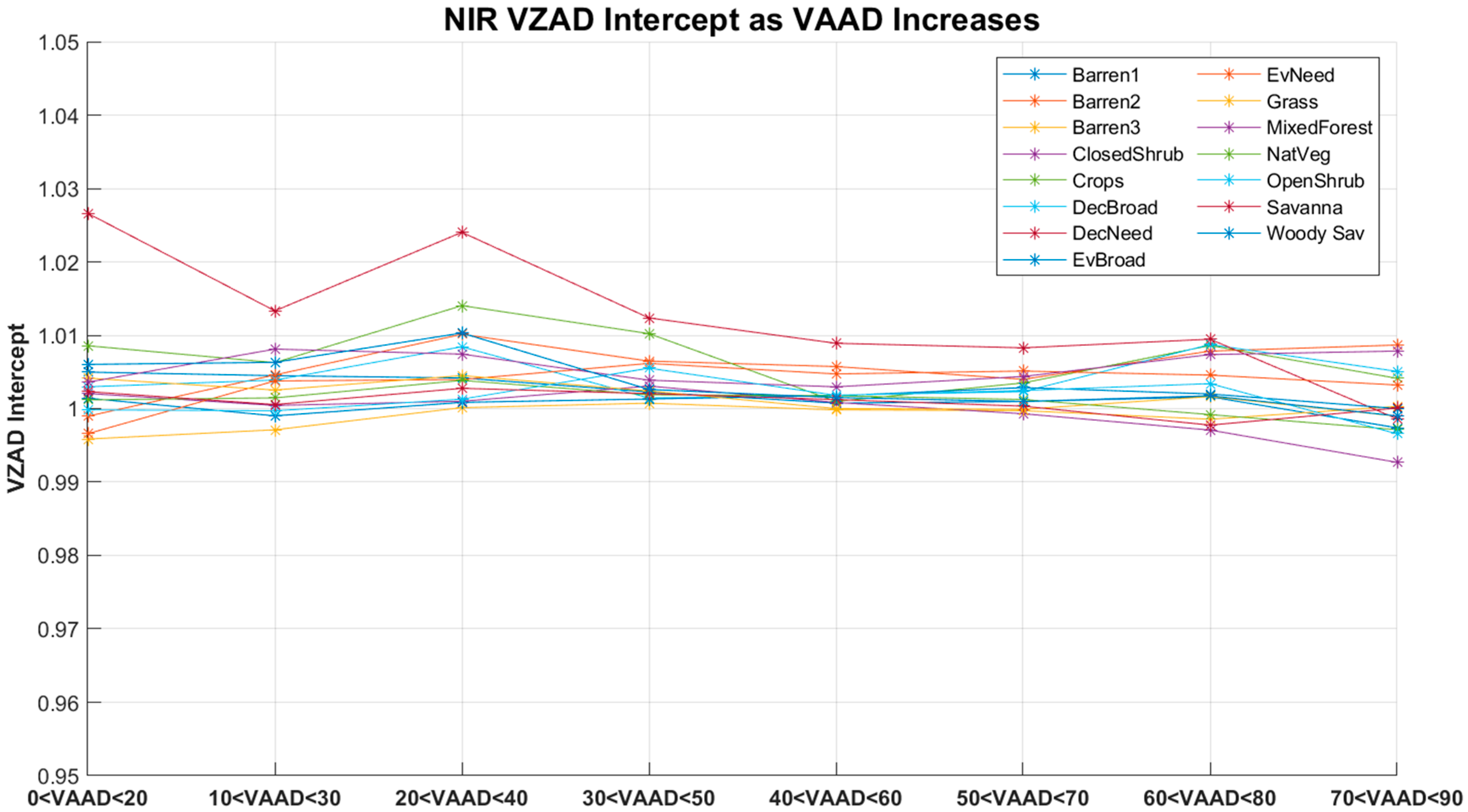
Figure 12.
The VZAD intercept for all IGBP types as VAAD increases from 0–90° in the NIR band. Note how the intercepts are about ±1% for all VZAD slices, except for the Deciduous Needleleaf class, which has a very low SNR, which likely drives its atypical performance. The “tightest” VAAD slice appeared to be the 50 < VAAD < 70 range, which had the greatest number of samples during the underfly, so a t-test was performed to test if the other VAAD slices were statistically similar to it.
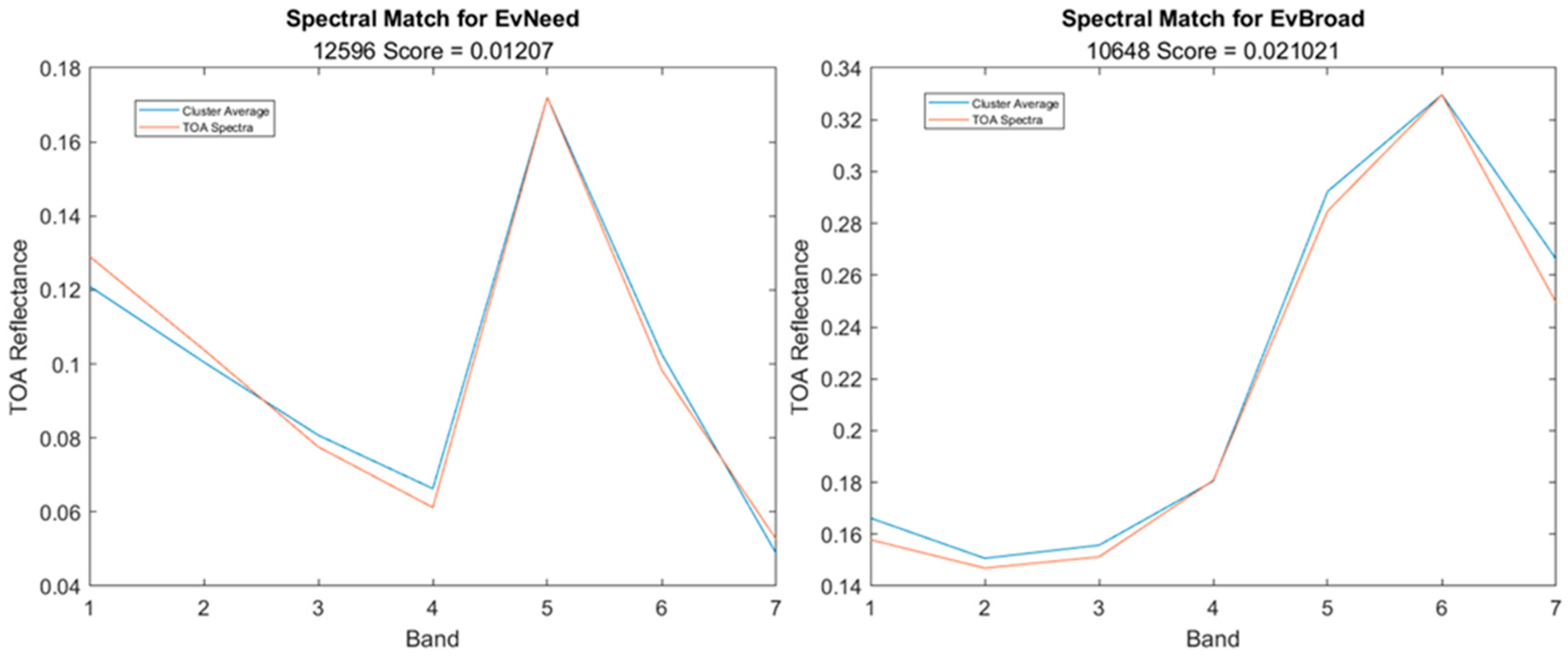
Figure 13.
IGBP to Banded hyperspectral signature matched examples. Note the score in the subtitles of the plots, as it is the resulting value from Equation (4). The lower the value, the closer the spectral match of the IGBP profile to the spectral library profile. The results show the spectra are about one to two reflectance units different from their corresponding match. The number to the left of the score signifies the sample in the spectral library used to match.
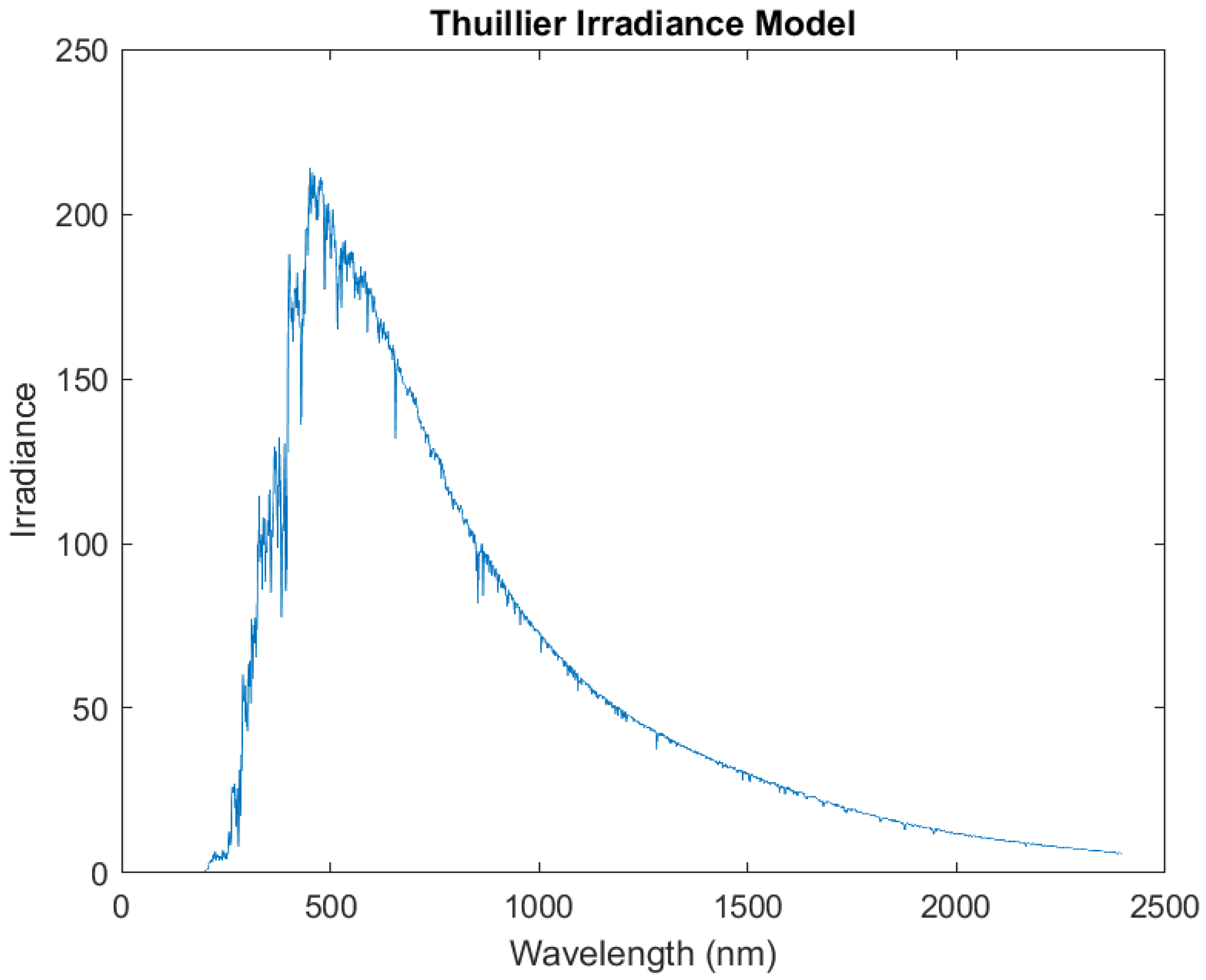
Figure 14.
Thullier irradiance model. This irradiance was applied to the reflectance curves in the SDSU-compiled spectral library to determine the radiance of each sample.
Figure 14.
Thullier irradiance model. This irradiance was applied to the reflectance curves in the SDSU-compiled spectral library to determine the radiance of each sample.
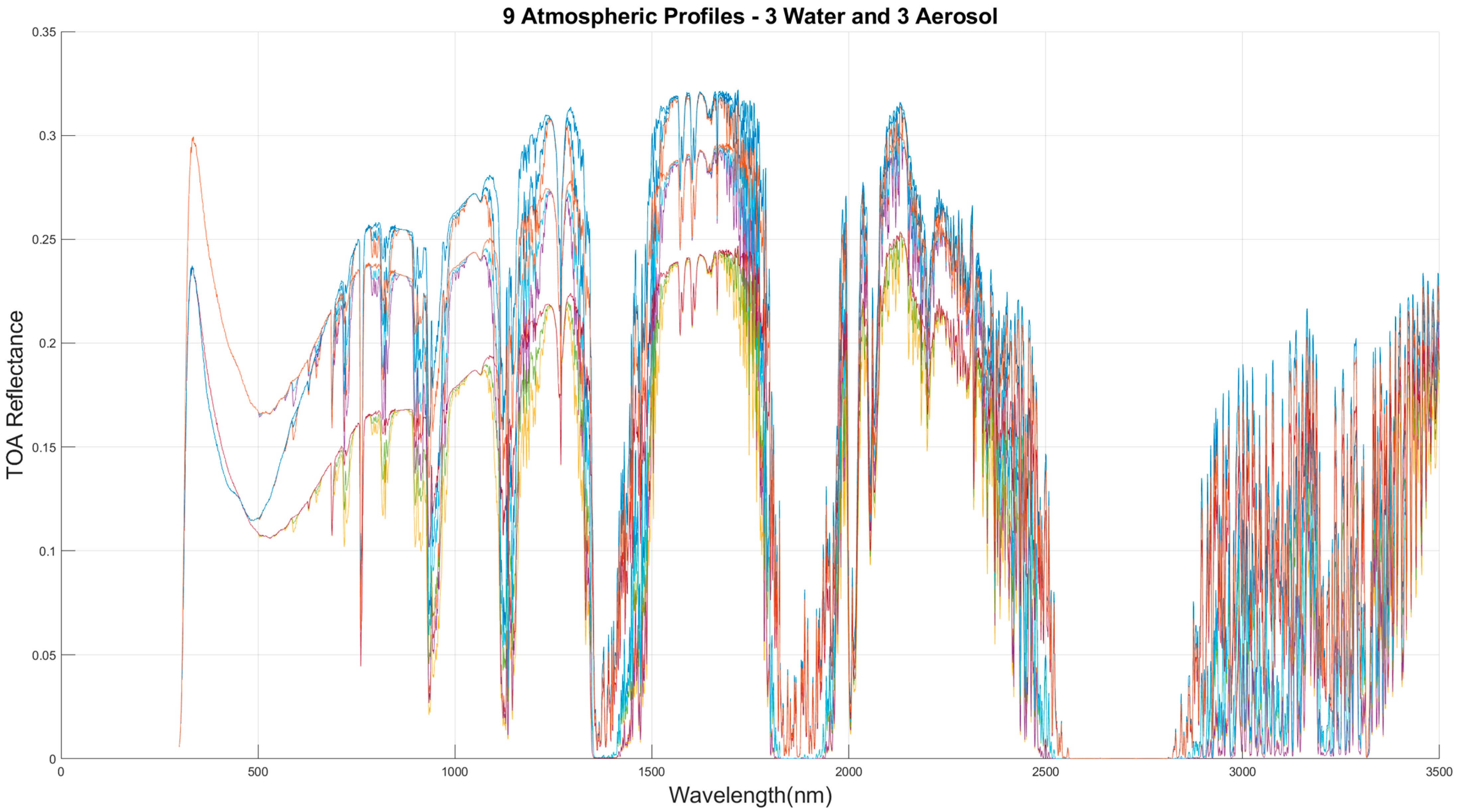
Figure 15.
Barren3 atmospheric profiles for spectral uncertainty analysis. Note there are three aerosol profiles and three water absorption profiles, which, combined, give a total of nine combinations. This large range of atmospheric profiles gave the spectral uncertainty analysis enough simulations to cover all possible scenarios during the underfly.
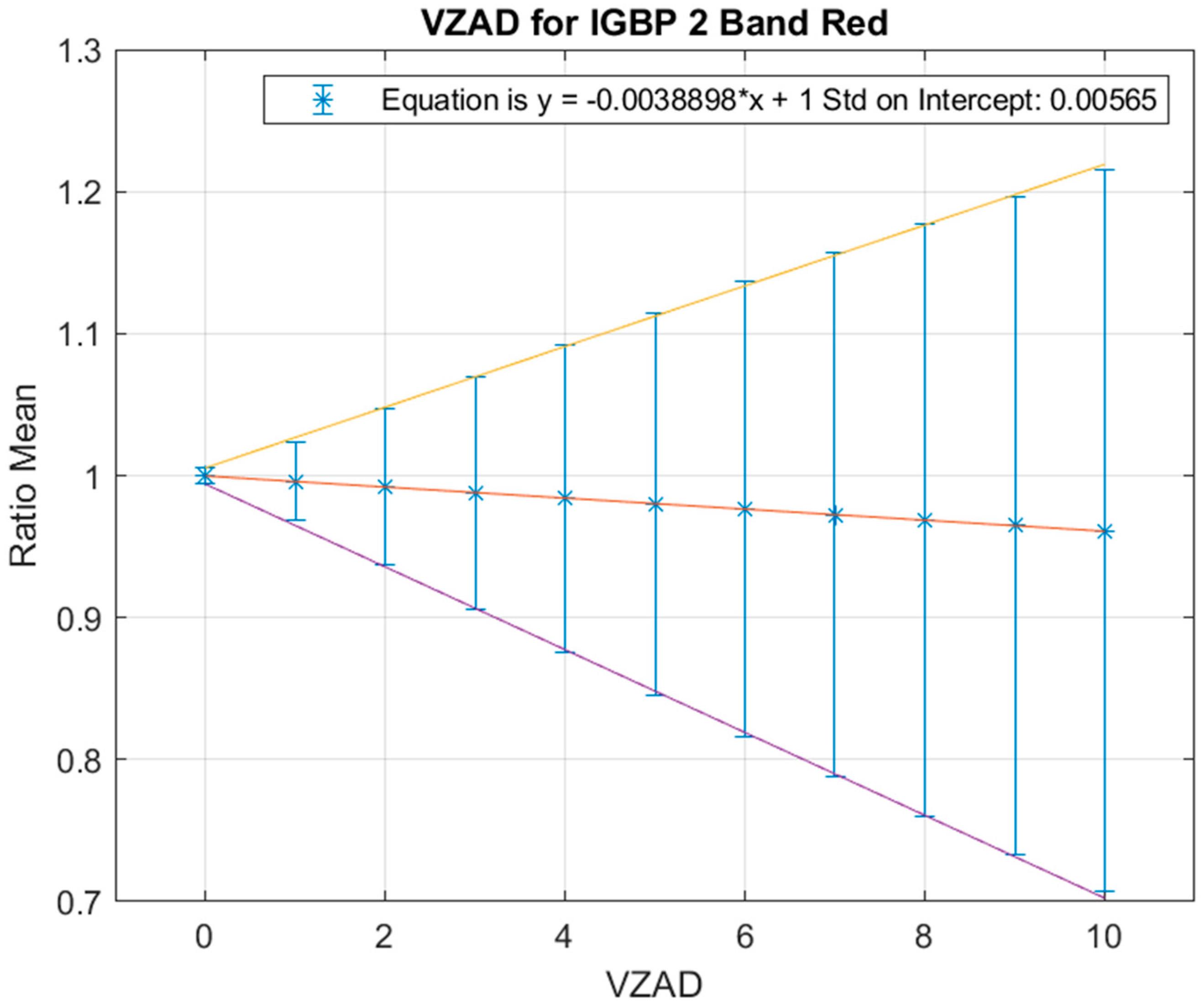
Figure 16.
BRDF uncertainty at the VZAD intercept. Note that the “bowtie” effect is prominent when looking at the BRDF uncertainties while exclusively in the principal plane, which gave the worst-case scenario for uncertainty. The error bars on the VZAD intercept are the estimated BRDF uncertainty at VZAD = 0° based on the uncertainties of VZADs = 1–10°. This value was averaged with the VZAD intercept uncertainties of every IGBP type in each band to find the overall BRDF uncertainty for all the bands.
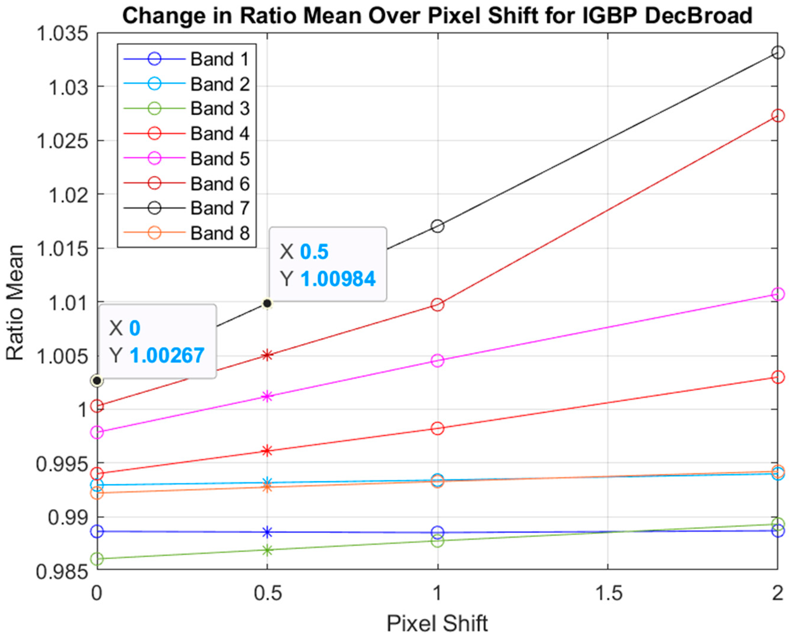
Figure 17.
Geometric bias plot. Pixel shift 0 has an uncertainty of ~1/3 pixel, so the bias introduced at that value needed to be determined. The ratio value between 0 and 1 at 0.5 was interpolated, denoted by *. Since the bias at pixel 0.5 is likely larger or equal to the bias introduced at ~1/3, that value was used to overestimate the bias as a worst-case scenario. The difference between 1.00984 and 1.00267 was determined to be the geometric bias on the SWIR2 band, being 0.00717.
Table 1.
Landsat 8 bands.
Table 1.
Landsat 8 bands.
| Bands | Wavelengths
(Micrometers) | Resolution
(Meters) |
|---|
| Band 1—Coastal Aerosol | 0.43–0.45 | 30 |
| Band 2—Blue | 0.45–0.51 | 30 |
| Band 3—Green | 0.53–0.59 | 30 |
| Band 4—Red | 0.64–0.67 | 30 |
| Band 5—Near Infrared (NIR) | 0.85–0.88 | 30 |
| Band 6—Short Wave Infrared 1 (SWIR1) | 1.57–1.65 | 30 |
| Band 7—SWIR2 | 2.11–2.29 | 30 |
| Band 8—Panchromatic Band | 0.50–0.68 | 15 |
| Band 9—Cirrus | 1.36–1.38 | 30 |
| Band 10—Thermal Infrared 1 (TIRS 1) | 10.6–11.19 | 100 |
| Band 11—TIRS 2 | 11.5–12.51 | 100 |
Table 2.
IGBP land cover types.
Table 2.
IGBP land cover types.
| Name | Value | Description |
|---|
| Evergreen Needleleaf Forests | 1 | Dominated by evergreen conifer trees (canopy > 2 m). Tree cover > 60%. |
| Evergreen Broadleaf Forests | 2 | Dominated by evergreen broadleaf and palmate trees (canopy > 2 m). Tree cover > 60%. |
| Deciduous Needleleaf Forests | 3 | Dominated by deciduous needleleaf (larch) trees (canopy > 2 m). Tree cover > 60%. |
| Deciduous Broadleaf Forests | 4 | Dominated by deciduous broadleaf trees (canopy > 2 m). Tree cover > 60%. |
| Mixed Forests | 5 | Dominated by neither deciduous nor evergreen (40–60% of each) tree type (canopy > 2 m). Tree cover > 60%. |
| Closed Shrublands | 6 | Dominated by woody perennials (1–2 m height) > 60% cover. |
| Open Shrublands | 7 | Dominated by woody perennials (1–2 m height) 10–60% cover. |
| Woody Savannas | 8 | Tree cover 30–60% (canopy > 2 m). |
| Savannas | 9 | Tree cover 10–30% (canopy > 2 m). |
| Grasslands | 10 | Dominated by herbaceous annuals (<2 m). |
| Permanent Wetlands | 11 | Permanently inundated lands with 30–60% water cover and >10% vegetated cover. |
| Croplands | 12 | At least 60% of area is cultivated cropland. |
| Urban and Built-up Lands | 13 | At least 30% impervious surface area including building materials, asphalt, and vehicles. |
| Cropland/Natural Vegetation Mosaics | 14 | Mosaics of small-scale cultivation 40–60% with natural tree, shrub, or herbaceous vegetation. |
| Permanent Snow and Ice | 15 | At least 60% of area is covered by snow and ice for at least 10 months of the year. |
| Barren | 16 | At least 60% of area is non-vegetated barren (sand, rock, soil) areas with less than 10% vegetation. |
| Water Bodies | 17 | At least 60% of area is covered by permanent water bodies. Has not received a map label because of missing inputs. |
Table 3.
TOA reflectance profiles for IGBP types.
Table 3.
TOA reflectance profiles for IGBP types.
| IGBP | 1 | 2 | 3 | 4 | 5 | 6 | 7 | 8 | 9 | 10 | 12 | 14 |
|---|
| Blue | 0.103 | 0.147 | 0.072 | 0.129 | 0.120 | 0.097 | 0.127 | 0.121 | 0.129 | 0.120 | 0.131 | 0.126 |
| Green | 0.076 | 0.151 | 0.053 | 0.109 | 0.113 | 0.086 | 0.128 | 0.114 | 0.129 | 0.111 | 0.111 | 0.131 |
| Red | 0.058 | 0.181 | 0.048 | 0.103 | 0.121 | 0.107 | 0.185 | 0.124 | 0.147 | 0.119 | 0.101 | 0.161 |
| NIR | 0.179 | 0.291 | 0.075 | 0.209 | 0.228 | 0.195 | 0.285 | 0.231 | 0.242 | 0.201 | 0.198 | 0.264 |
| SWIR1 | 0.116 | 0.339 | 0.037 | 0.170 | 0.216 | 0.261 | 0.372 | 0.233 | 0.267 | 0.221 | 0.167 | 0.278 |
| SWIR2 | 0.055 | 0.262 | 0.021 | 0.117 | 0.148 | 0.195 | 0.306 | 0.164 | 0.199 | 0.157 | 0.099 | 0.220 |
Table 4.
Separated barren reflectance profiles.
Table 4.
Separated barren reflectance profiles.
| IGBP | Barren1 | Barren2 | Barren3 | Barren4 |
|---|
| Blue | 0.097 | 0.098 | 0.169 | 0.137 |
| Green | 0.095 | 0.084 | 0.201 | 0.124 |
| Red | 0.105 | 0.067 | 0.276 | 0.132 |
| NIR | 0.139 | 0.213 | 0.375 | 0.217 |
| SWIR1 | 0.178 | 0.142 | 0.457 | 0.264 |
| SWIR2 | 0.153 | 0.071 | 0.398 | 0.201 |
Table 5.
Reflectance cross-calibration gain estimates for each IGBP type before SBAF correction.
Table 5.
Reflectance cross-calibration gain estimates for each IGBP type before SBAF correction.
| Cross-Cal Gains | Barren1 | Barren2 | Barren3 | ClosedShrub | Crops | DecBroad | DecNeed | EvBroad |
| Band | Mean | ±Sigma | Mean | ±Sigma | Mean | ±Sigma | Mean | ±Sigma | Mean | ±Sigma | Mean | ±Sigma | Mean | ±Sigma | Mean | ±Sigma |
| CA | 1.000 | 0.014 | 0.999 | 0.014 | 0.997 | 0.021 | 0.999 | 0.012 | 0.998 | 0.016 | 0.999 | 0.013 | 1.000 | 0.014 | 1.000 | 0.015 |
| Blue | 1.001 | 0.016 | 1.000 | 0.015 | 0.998 | 0.026 | 1.000 | 0.014 | 1.000 | 0.018 | 1.001 | 0.016 | 1.001 | 0.017 | 1.002 | 0.019 |
| Green | 0.996 | 0.020 | 0.993 | 0.021 | 0.997 | 0.033 | 0.995 | 0.017 | 0.994 | 0.028 | 0.995 | 0.025 | 0.992 | 0.024 | 0.999 | 0.024 |
| Red | 1.002 | 0.029 | 1.001 | 0.027 | 0.997 | 0.032 | 0.998 | 0.019 | 0.999 | 0.036 | 1.001 | 0.034 | 1.000 | 0.038 | 1.001 | 0.031 |
| NIR | 1.003 | 0.031 | 1.005 | 0.028 | 0.998 | 0.024 | 0.999 | 0.023 | 1.002 | 0.031 | 1.001 | 0.029 | 1.008 | 0.054 | 1.001 | 0.026 |
| SWIR1 | 1.010 | 0.045 | 1.014 | 0.037 | 0.997 | 0.026 | 1.002 | 0.021 | 1.008 | 0.055 | 1.007 | 0.040 | 1.020 | 0.069 | 1.002 | 0.027 |
| SWIR2 | 1.009 | 0.040 | 1.018 | 0.054 | 0.997 | 0.032 | 1.000 | 0.029 | 1.009 | 0.060 | 1.007 | 0.089 | 1.028 | 0.082 | 1.001 | 0.035 |
| Pan | 1.002 | 0.019 | 0.996 | 0.021 | 1.005 | 0.038 | 1.000 | 0.015 | 0.993 | 0.022 | 1.000 | 0.015 | 0.968 | 0.034 | 1.005 | 0.023 |
| | | EvNeed | Grass | MixedFor | NatVeg | OpenShrub | Savanna | WoodySav | |
| | Band | Mean | ±Sigma | Mean | ±Sigma | Mean | ±Sigma | Mean | ±Sigma | Mean | ±Sigma | Mean | ±Sigma | Mean | ±Sigma | |
| | CA | 0.999 | 0.014 | 1.000 | 0.013 | 1.000 | 0.015 | 0.999 | 0.013 | 0.999 | 0.019 | 0.999 | 0.012 | 1.000 | 0.015 | |
| | Blue | 1.001 | 0.014 | 1.001 | 0.014 | 1.002 | 0.018 | 1.001 | 0.015 | 1.001 | 0.021 | 1.000 | 0.020 | 1.002 | 0.018 | |
| | Green | 0.992 | 0.021 | 0.996 | 0.017 | 0.996 | 0.028 | 0.998 | 0.020 | 1.000 | 0.022 | 0.996 | 0.022 | 0.997 | 0.024 | |
| | Red | 0.999 | 0.031 | 1.000 | 0.022 | 1.003 | 0.026 | 1.000 | 0.030 | 1.000 | 0.022 | 1.000 | 0.022 | 1.003 | 0.032 | |
| | NIR | 1.004 | 0.039 | 1.001 | 0.024 | 1.004 | 0.024 | 1.001 | 0.022 | 1.000 | 0.017 | 1.001 | 0.022 | 1.004 | 0.027 | |
| | SWIR1 | 1.011 | 0.052 | 1.005 | 0.027 | 1.011 | 0.034 | 1.002 | 0.027 | 0.999 | 0.019 | 1.003 | 0.025 | 1.009 | 0.034 | |
| | SWIR2 | 1.016 | 0.051 | 1.003 | 0.032 | 1.012 | 0.041 | 1.001 | 0.034 | 0.999 | 0.024 | 1.002 | 0.031 | 1.010 | 0.043 | |
| | Pan | 0.984 | 0.024 | 1.001 | 0.019 | 1.001 | 0.019 | 1.003 | 0.017 | 1.006 | 0.018 | 1.003 | 0.016 | 1.004 | 0.016 | |
Table 6.
Inverse-weighted mean variance estimation before SBAF correction.
Table 6.
Inverse-weighted mean variance estimation before SBAF correction.
| | Weighted
Variance
Estimator |
|---|
| Band | Mean | Std Dev |
|---|
| CA | 0.999 | 0.004 |
| Blue | 1.001 | 0.004 |
| Green | 0.996 | 0.006 |
| Red | 1.000 | 0.007 |
| NIR | 1.001 | 0.007 |
| SWIR1 | 1.004 | 0.008 |
| SWIR2 | 1.004 | 0.010 |
| Pan | 1.000 | 0.005 |
Table 7.
SBAFs for each of the IGBP land cover types.
Table 7.
SBAFs for each of the IGBP land cover types.
| IGBP | CA | Blue | Green | Red | NIR | SWIR1 | SWIR2 | Pan |
|---|
| EvNeed | 0.998 | 0.999 | 0.998 | 1.000 | 1.000 | 1.001 | 1.004 | 1.005 |
| EvBroad | 0.999 | 1.000 | 1.000 | 1.001 | 1.000 | 1.001 | 1.001 | 0.997 |
| DecNeed | 0.998 | 0.999 | 0.998 | 1.000 | 1.000 | 1.001 | 1.003 | 1.006 |
| DecBroad | 0.998 | 0.999 | 0.998 | 1.000 | 1.000 | 1.001 | 1.002 | 1.004 |
| Mixedfor | 0.999 | 0.999 | 0.998 | 1.000 | 1.000 | 1.002 | 1.002 | 1.005 |
| ClosedShrub | 0.999 | 1.000 | 0.999 | 1.001 | 1.000 | 1.001 | 1.002 | 1.000 |
| OpenShrub | 0.999 | 0.999 | 1.001 | 1.001 | 1.000 | 1.000 | 1.000 | 0.992 |
| WoodySav | 0.998 | 0.999 | 0.998 | 1.000 | 1.000 | 1.001 | 1.002 | 1.003 |
| Savanna | 0.999 | 1.000 | 0.999 | 1.001 | 1.000 | 1.001 | 1.001 | 0.999 |
| Grass | 0.998 | 0.999 | 0.999 | 1.001 | 1.000 | 1.001 | 1.001 | 0.999 |
| Crops | 0.999 | 0.999 | 0.999 | 1.000 | 1.000 | 1.002 | 1.003 | 1.003 |
| NatVeg | 0.999 | 1.000 | 0.999 | 1.001 | 1.000 | 1.001 | 1.002 | 1.000 |
| Barren1 | 0.998 | 0.999 | 0.999 | 1.001 | 1.000 | 1.001 | 1.001 | 0.999 |
| Barren2 | 0.998 | 0.999 | 0.998 | 0.999 | 1.000 | 1.002 | 1.003 | 1.009 |
| Barren3 | 1.000 | 1.000 | 1.002 | 1.001 | 1.000 | 1.000 | 1.000 | 0.992 |
Table 8.
SBAF-corrected cross-calibration gains. The inverse-weighted mean variance estimation results were the values recommended to USGS EROS for final reflectance cross-calibration. Note how the values are within 0.5% of unity, which further supports how effective Phase 1 was.
Table 8.
SBAF-corrected cross-calibration gains. The inverse-weighted mean variance estimation results were the values recommended to USGS EROS for final reflectance cross-calibration. Note how the values are within 0.5% of unity, which further supports how effective Phase 1 was.
SBAF
Corrected Gains | Barren1 | Barren2 | Barren3 | ClosedShrub | Crops | DecBroad | DecNeed | EvBroad |
| Band | Mean | ±Sigma | Mean | ±Sigma | Mean | ±Sigma | Mean | ±Sigma | Mean | ±Sigma | Mean | ±Sigma | Mean | ±Sigma | Mean | ±Sigma |
| CA | 1.001 | 0.014 | 1.001 | 0.015 | 0.997 | 0.021 | 1.001 | 0.012 | 1.000 | 0.016 | 1.001 | 0.013 | 1.002 | 0.014 | 1.001 | 0.015 |
| Blue | 1.002 | 0.016 | 1.002 | 0.015 | 0.998 | 0.026 | 1.000 | 0.014 | 1.001 | 0.018 | 1.002 | 0.016 | 1.002 | 0.017 | 1.003 | 0.019 |
| Green | 0.997 | 0.020 | 0.995 | 0.021 | 0.995 | 0.033 | 0.996 | 0.017 | 0.995 | 0.028 | 0.996 | 0.025 | 0.993 | 0.024 | 0.999 | 0.024 |
| Red | 1.001 | 0.029 | 1.001 | 0.027 | 0.996 | 0.032 | 0.998 | 0.019 | 0.999 | 0.036 | 1.001 | 0.034 | 1.000 | 0.038 | 1.000 | 0.030 |
| NIR | 1.003 | 0.031 | 1.005 | 0.028 | 0.998 | 0.024 | 0.999 | 0.023 | 1.002 | 0.031 | 1.001 | 0.029 | 1.008 | 0.054 | 1.001 | 0.026 |
| SWIR1 | 1.009 | 0.045 | 1.011 | 0.037 | 0.997 | 0.026 | 1.001 | 0.021 | 1.006 | 0.055 | 1.005 | 0.040 | 1.018 | 0.069 | 1.001 | 0.027 |
| SWIR2 | 1.008 | 0.040 | 1.015 | 0.054 | 0.996 | 0.032 | 0.999 | 0.029 | 1.006 | 0.060 | 1.005 | 0.089 | 1.026 | 0.082 | 1.000 | 0.035 |
| Pan | 1.003 | 0.019 | 0.988 | 0.021 | 1.013 | 0.038 | 1.000 | 0.015 | 0.989 | 0.022 | 0.996 | 0.014 | 0.962 | 0.034 | 1.009 | 0.023 |
| | EvNeed | Grass | MixedFor | NatVeg | OpenShrub | Savanna | WoodySav | Inverse-Weighted Variance Estimator |
| Band | Mean | ±Sigma | Mean | ±Sigma | Mean | ±Sigma | Mean | ±Sigma | Mean | ±Sigma | Mean | ±Sigma | Mean | ±Sigma | Mean | Std Dev |
| CA | 1.000 | 0.015 | 1.001 | 0.013 | 1.001 | 0.015 | 1.001 | 0.013 | 1.000 | 0.019 | 1.000 | 0.012 | 1.002 | 0.015 | 1.001 | 0.004 |
| Blue | 1.002 | 0.014 | 1.001 | 0.014 | 1.002 | 0.018 | 1.002 | 0.015 | 1.002 | 0.021 | 1.001 | 0.020 | 1.002 | 0.018 | 1.002 | 0.004 |
| Green | 0.994 | 0.021 | 0.996 | 0.017 | 0.998 | 0.028 | 0.998 | 0.020 | 0.999 | 0.022 | 0.997 | 0.022 | 0.998 | 0.024 | 0.996 | 0.006 |
| Red | 0.999 | 0.031 | 0.999 | 0.022 | 1.003 | 0.026 | 1.000 | 0.030 | 0.999 | 0.022 | 0.999 | 0.022 | 1.002 | 0.032 | 1.000 | 0.007 |
| NIR | 1.004 | 0.039 | 1.001 | 0.024 | 1.004 | 0.024 | 1.000 | 0.022 | 1.000 | 0.017 | 1.000 | 0.022 | 1.003 | 0.027 | 1.001 | 0.007 |
| SWIR1 | 1.009 | 0.052 | 1.004 | 0.027 | 1.009 | 0.034 | 1.000 | 0.027 | 0.999 | 0.019 | 1.002 | 0.025 | 1.008 | 0.034 | 1.003 | 0.008 |
| SWIR2 | 1.013 | 0.050 | 1.002 | 0.032 | 1.009 | 0.041 | 1.000 | 0.034 | 0.999 | 0.024 | 1.001 | 0.031 | 1.008 | 0.042 | 1.002 | 0.010 |
| Pan | 0.978 | 0.023 | 1.002 | 0.019 | 0.997 | 0.019 | 1.004 | 0.017 | 1.015 | 0.018 | 1.004 | 0.016 | 1.001 | 0.016 | 0.999 | 0.005 |
Table 9.
Radiance SBAF-corrected cross-calibration gain estimates. These values are further from unity than the reflectance values, which was the main focus of Phase 1.
Table 9.
Radiance SBAF-corrected cross-calibration gain estimates. These values are further from unity than the reflectance values, which was the main focus of Phase 1.
| | Inverse-Weighted Variance
Estimator |
| Band | Mean | Std Dev |
| CA | 1.001 | 0.004 |
| Blue | 0.999 | 0.004 |
| Green | 0.997 | 0.006 |
| Red | 0.996 | 0.007 |
| NIR | 0.996 | 0.007 |
| SWIR1 | 0.992 | 0.008 |
| SWIR2 | 0.990 | 0.010 |
| Pan | 0.996 | 0.005 |
| Band 10 | 0.998 | 0.008 |
| Band 11 | 1.010 | 0.008 |
Table 10.
Spectral uncertainty table. Uncertainty units are reflectance.
Table 10.
Spectral uncertainty table. Uncertainty units are reflectance.
| Band | CA | Blue | Green | Red | NIR | SWIR1 | SWIR2 | Pan |
|---|
| Ratio Mean | 0.9989 | 0.9995 | 0.9992 | 1.0004 | 1.0001 | 1.0011 | 1.0013 | 1.0009 |
| Uncertainty | 0.0012 | 0.0007 | 0.0010 | 0.0007 | 0.0008 | 0.0017 | 0.0015 | 0.0022 |
Table 11.
BRDF uncertainty table.
Table 11.
BRDF uncertainty table.
| Band | CA | Blue | Green | Red | NIR | SWIR1 | SWIR2 | Pan |
|---|
| Uncertainty | 0.0007 | 0.0011 | 0.0024 | 0.0015 | 0.0026 | 0.0017 | 0.0009 | 0.0017 |
Table 12.
Geometric bias table.
Table 12.
Geometric bias table.
| Band | CA | Blue | Green | Red | NIR | SWIR1 | SWIR2 | Pan |
|---|
| Uncertainty | 0.0001 | 0.0002 | 0.0006 | 0.0020 | 0.0055 | 0.0080 | 0.0081 | 0.0007 |
Table 13.
Total uncertainty table.
Table 13.
Total uncertainty table.
| Band | CA | Blue | Green | Red | NIR | SWIR1 | SWIR2 | Pan |
|---|
| Uncertainty | 0.0014 | 0.0013 | 0.0027 | 0.0026 | 0.0062 | 0.0084 | 0.0083 | 0.0029 |


