Article

InSAR-Based Early Warning Monitoring Framework to Assess Aquifer Deterioration

1
Department of Civil, Building and Environmental Engineering (DICEA), Sapienza University of Rome, 00185 Rome, Italy
2
Department of Water Resources, Faculty of Agricultural Engineering, University of Concepción, Chillan 3780000, Chile
3
Department of Civil Engineering, University of Concepcion, Concepcion 4070409, Chile
4
Water Resources Center for Agriculture and Mining (CRHIAM), University of Concepcion, Concepcion 4089100, Chile
*
Author to whom correspondence should be addressed.
Remote Sens. 2023, 15(7), 1786; https://doi.org/10.3390/rs15071786
Submission received: 21 February 2023 / Revised: 16 March 2023 / Accepted: 22 March 2023 / Published: 27 March 2023
(This article belongs to the Special Issue Remote Sensing Approaches to Groundwater Management and Mapping)

Abstract

:
Aquifer surveillance is key to understanding the dynamics of groundwater reservoirs. Attention should be focused on developing strategies to monitor and mitigate the adverse consequences of overexploitation. In this context, ground surface deformation monitoring allows us to estimate the spatial and temporal distribution of groundwater levels, determine the recharge times of the aquifers, and calibrate the hydrological models. This study proposes a methodology for implementing advanced multitemporal differential interferometry (InSAR) techniques for water withdrawal surveillance and early warning assessment. For this, large open-access images were used, a total of 145 SAR images from the Sentinel 1 C-band satellite provided by the Copernicus mission of the European Space Agency. InSAR processing was carried out with an algorithm based on parallel computing technology implemented in cloud infrastructure, optimizing complex workflows and processing times. The surveillance period records 6-years of satellite observation from September 2016 to December 2021 over the city of Chillan (Chile), an area exposed to urban development and intensive agriculture, where ~80 wells are located. The groundwater flow path spans from the Andes Mountain range to the Pacific Ocean, crossing the Itata river basin in the Chilean central valley. InSAR validation measurements were carried out by comparing the results with the values of continuous GNSS stations available in the area of interest. The performance analysis is based on spatial analysis, time series, meteorological stations data, and static level measurements, as well as hydrogeological structure. The results indicate seasonal variations in winter and summer, which corresponds to the recovery and drawdown periods with velocities > −10 mm/year, and an aquifer deterioration trend of up to 60 mm registered in the satellite SAR observation period. Our results show an efficient tool to monitor aquifer conditions, including irreversible consolidation and storage capacity loss, allowing timely decision making to avoid harmful exploitation.

Graphical Abstract

1. Introduction

Land subsidence, which refers to the sinking of the land surface due to natural or anthropogenic processes related to aquifer depletion, has become a pressing global issue [1,2]. The rate of land subsidence is accelerating in many parts of the world due to increased groundwater extraction and the loss of support provided by the overlying soil layer, caused by mining and urban construction activities [3,4]. Furthermore, with climate change being a major environmental concern, the potential for increased drought and rainfall events could also exacerbate the impacts of land subsidence due to the overexploitation of groundwater resources [5]. It has already been shown that the combination of these factors can modify aquifer balances and the structure of the aquifer system in itself [6,7]. This has not only raised concerns relating to the vulnerability of existing infrastructure to damage from land subsidence in the future, but also to the possible increase in environmental problems such as changes in rivers, canals, and drawing flow systems and flooding risk in low-lying areas, as well as the decrease in groundwater levels used for irrigation and human consumption, increases in inland seawater intrusion, and the deterioration of soil and water conditions, affecting groundwater-dependent ecosystems [8,9,10].
Land subsidence can occur slowly without being noticed by the local population until the consequences are severe enough. Therefore, it is important to develop an effective early warning surveillance system based on remote sensing data that can monitor changes in groundwater levels and provide timely information that can be used to mitigate potential impacts, as well as serve as a tool for correct water management.
Many approaches have been developed for the study of aquifer compaction, including the fundamental relationship between groundwater head, water flow direction, water pressure, and aquifer compaction [11]. The results of these studies have allowed solving the compaction process with respect to the drainage age [12].The theoretical models used today are usually complicated and require many resources. Therefore, it is noted that more research is needed for more efficient modeling of drainage-induced ground surface displacement [13].
Ground deformations surveillance is a resource-intensive task and must be achieved by using traditional ground-based techniques. Ground displacement can be performed based on in situ instrumentation such as GNSS or traditional surveying, which provide reliable measurements to monitor subsidence [14]. However, they are limited due to logistics and costs, as well as in terms of spatial coverage. The use of satellite radar interferometry monitoring in aquifer studies represents an important advance, due to its high millimeter precision, its low cost, and optimal spatial and temporal coverage. In particular, SAR remote sensing data acquired by Synthetic Aperture Radar (SAR) satellite sensors and processed through Differential Interferometry SAR (InSAR) techniques, greatly contribute to surface deformation analyses [15,16,17]. These have been used mainly in the geophysical [18,19], volcanic [20,21], or even for infrastructure monitoring [22,23]. In recent years, many InSAR studies have been developed, illustrating large deformations in aquifer compaction [24,25,26,27,28]; however, it is possible to explore InSAR for early warning surveillance, considering the accuracy of the measurements, the continuous updating of Sentinel 1 open data, and the rapid results of SAR image processing with a cloud computing infrastructure.
The InSAR multitemporal technique allows measuring ground displacement using the phase difference with a series of interferograms generated at different times in the same area [15]. InSAR implementation seems to be one of the most promising techniques for monitoring aquifers, since it allows monitoring the ground surface remotely and with updated SAR images. The rapid development of InSAR technology has contributed to significant progress in monitoring drainage-related land surface deformation [29]. Combining InSAR results with in situ data makes a broader approach to water hazard assessment possible [30,31]. In addition, these techniques, due to their spatial coverage, allow us to identify and understand the phenomenon of aquifer compaction due to water withdrawals [32].
The use of InSAR makes it possible to determine the structural limits of aquifer systems, the spatiotemporal distribution of displacements, and the hydrogeological heterogeneity of the system, as well as estimates of storage coefficients [11]. The principles of InSAR technology are based on two coherent pixel selection approaches: the first is the Persistent Scatterers (PS) technique developed by Ferretti et al. [33], and the second is SBAS (Small BAseline Subset), developed by Bernardino et al. [34]. These approaches process multiple SAR images, providing displacement patterns over an observation period, collecting time series with centimeter and/or millimeter precision [35,36,37].
InSAR observations from satellites are becoming more reliable for long-term displacement monitoring in urban areas. The main contribution of this technique is the exploitation of a large number of observed point displacements, distributed throughout the landscape using open SAR images, becoming one of the most powerful and economical means; however, the measurements are not absolute, as they are relative with respect to a reference point located in the observed area. In this study we use the P-SBAS algorithm [38,39] developed by CNR—IREA (Italian Institute for Remote Sensing for the Environment). This approach is based on the principle of SBAS implemented in parallel computing and allows obtaining a long time series from a robust interferometric stack. The processing of the SAR images was carried out through the P-SBAS algorithm configured in the computing cloud of the Geohazard platform [40,41,42,43].
The advantage of using parallelization is to automate the processing chain of a very complex algorithm. This is undoubtedly decisive to obtain quick results for environmental surveillance and mitigation, decision making, and early warning surveillance, contributing to water sustainability and the development of future empirical models. Therefore, the proposed framework focuses on the rapid detection of the land deformations obtained from the satellite orbit. The results of this study show the behavior and the temporal and spatial variability of the aquifer, using the Line-Of-Sight (LOS) of the SAR sensor, and the production of velocities maps LOS [mm/year] and cumulative displacement [mm] in the area of the Central Valley of Chile. The analysis compares the measurements of the InSAR time series with continuous GNSS stations, static levels, and weather stations, confirming the potential of the technique for early warning surveillance from open access SAR images and the latest generation tools.

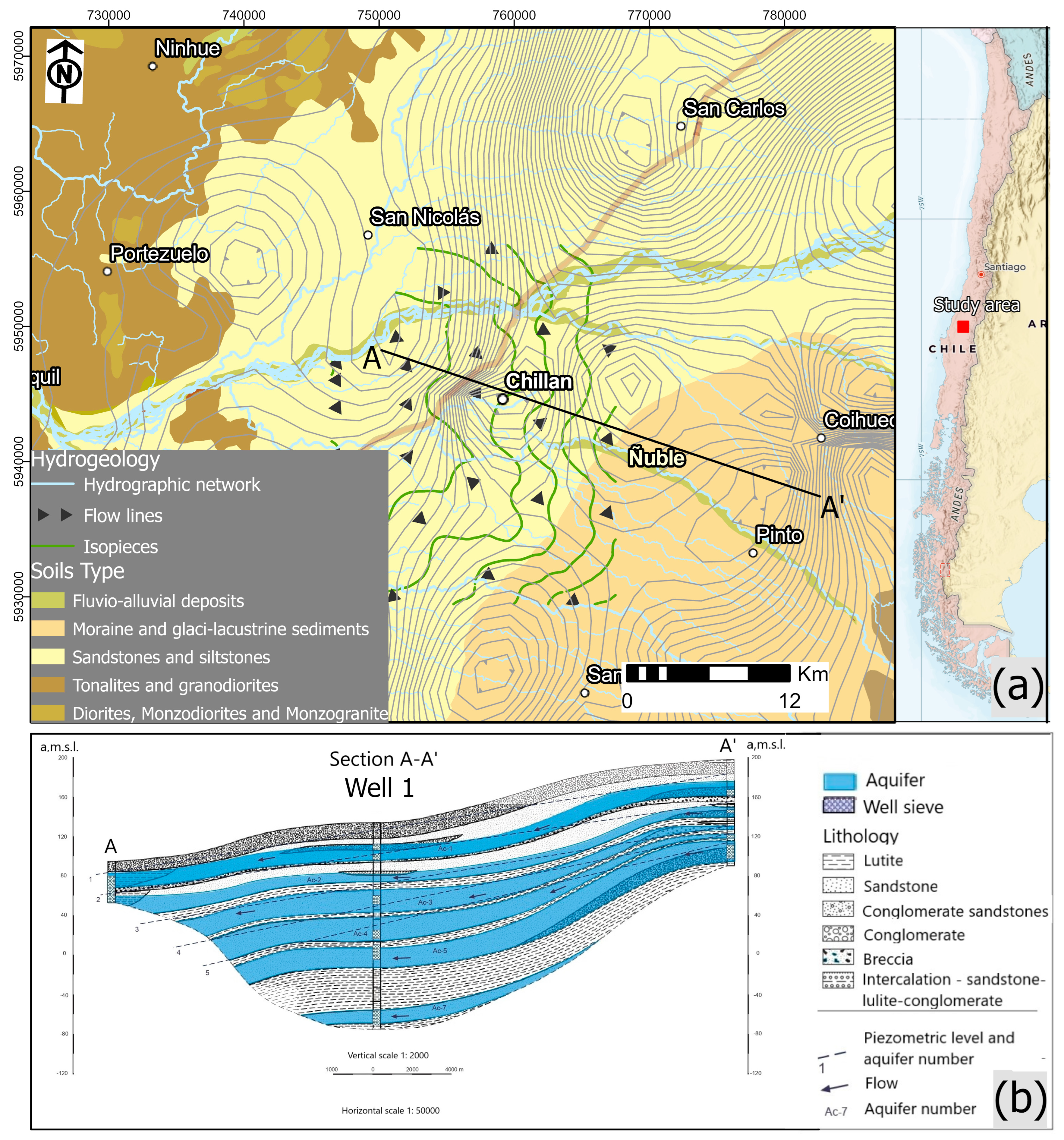
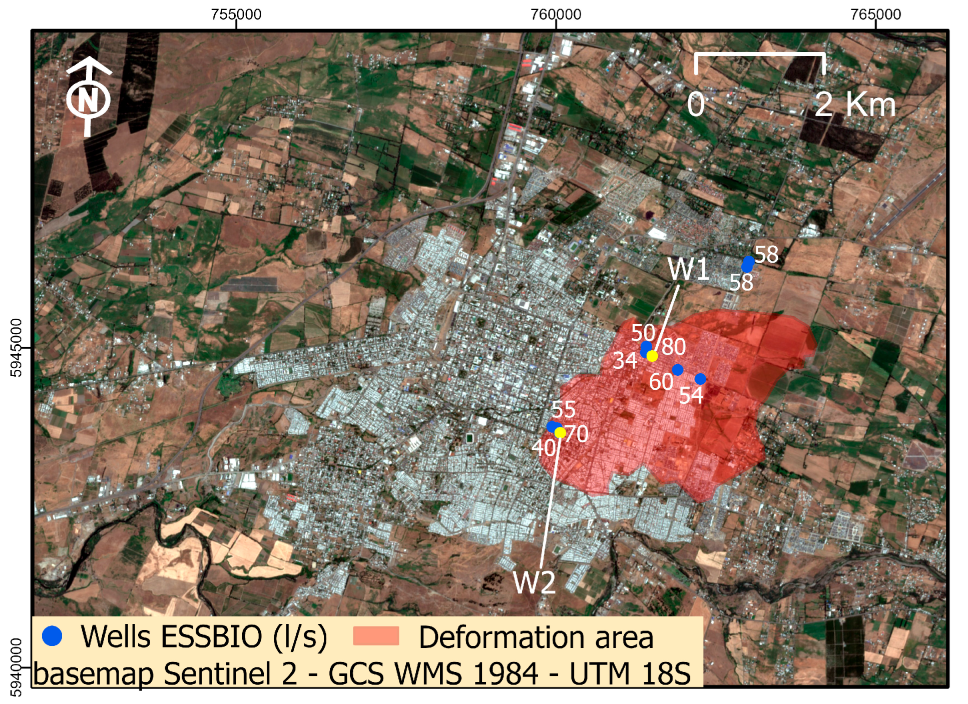
2. Study area and Hydrogeological Context

The study area is the town of Chillan, which is located in the Central Valley of Chile, west of the coastal mountain range and east of the Andes Mountain Range, within the hydrographic basin of the Itata River, between its tributary rivers (Ñuble and Larqui) (Figure 1). Specifically, it is located between the geographic coordinates 36°17′–36°54′ South Latitude and 71°43′–71°41′ West Longitude, covering approximately 2500 “km2” of extension.

Hydrogeological Context

The hydrogeological context of the study area is shown in the hydrogeological map (see Figure 2a). The hydrogeological section A-A′ (see Figure 2b) is composed of Paleozoic intrusive rocks, corresponding to the unit called South Coastal Batholith (BCS), and by Pleisto-Holocene sedimentary rocks that constitute the Mininco Formation. Petrographically, the intrusive is classified as granite and continuously outcrops to the NW of Estero Pataguas and Río Ñuble. It is considered a unit of low hydrogeological performance due to its anisotropic permeability, which depends on the magnitude, density, and geometry of the discontinuities, as well as the degree of alteration that the rock presents. On the other hand, the sediments of the Mininco Formation are widely distributed, are of fluvial and volcano-sedimentary origin, and are composed of an alternation of horizontal and lenticular strata with varied granulometry (clay, sand, and gravel), which frequently present lateral changes of lithofacies. With the lithostratigraphic information, an aquifer system composed of seven hydrogeological units (aquifers) housed in strata of the Mininco Formation is defined and characterized. The piezometric level varies from winter to summer, with a progressive decrease from East to West, while its depth is less than 15 m that otherwise has an average of 11.46 m in the study area. The direction of groundwater movement has a dominant E-W trajectory and coincides with the general patterns of surface flow [44].

3. Materials and Method

The method uses the InSAR multiple image approach of a parallel algorithm based on cloud technology together with in situ data on water extraction, the geological characteristics of the area, and hydrogeological interpretation of the phenomenon. The P-SBAS processing chain was properly developed to efficiently exploit the parallelism offered by modern computing platforms. The different distributed computing infrastructures available today, such as cluster, grid, and Cloud Computing (CC) [45,46], are suitable enough to be used effectively to process a large amount of Sentinel 1 data.
The P-SBAS processing chain modules addressed well-defined tasks within the remote sensing process, implementing parallelization strategies with reliable results. The method deals with the dynamics of reservoirs for groundwater management, with InSAR data, displacement maps (mm/year), and cumulative displacement maps (mm) generated for the summer and winter peaks, while the spatial deformation is performed with kriging spatial interpolation methods. In addition, GNSS measurements and InSAR with high coherence PSI, and InSAR measurements were compared with precipitation, the seasonal levels of the wells, and the hydrogeological structure of the study area.

3.1. InSAR Approach

The InSAR approach adopted to derive a time series of ground deformation in the study area is based on the principles of the SBAS method [34] defined below. The SBAS uses multi-interferograms produced from pairs of SAR images with high coherence, measuring the interferometric phase contained in the pixels of Sentinel 1. The interferometric phase is the sensor-target distance in the direction of the LOS. For each pixel, SBAS produces time-resolved ground deformation time-series from SAR images and millimeter-accuracy LOS velocity maps.
Considering a set of N SAR images acquired by Sentinel 1 over the study area, K interferograms with small temporal and spatial baselines are generated. For a given interferogram i in the interferogram stack, the observed phase of pixel x , y in the radar coordinates can be written as [33,34]:
o b s , i x , y = t o p o , i x , y + d e f , i x , y + a t m , i x , y + n o i s e , i x , y
where i refers to the i-th interferogram in the stack of differential interferograms (i ; [1,K]), t o p o , i is the residual topographic phase error due to inaccuracy of the reference DEM, d e f , i represents the phase caused by displacement of the pixel in the satellite LOS direction, a t m , i accounts for the phase contributed by the atmospheric inhomogeneities between two radar acquisition times, and n o i s e , i corresponds to the phase introduced by thermal noise and co-registration errors.
To achieve a better accuracy in estimation of ground deformation d e f , i , other components t o p o , i , a t m , i and n o i s e , i need to be accurately estimated and removed from the observed signal o b s , i . Therefore, the ground deformation time-series calculated with the SBAS method can be represented as follows:
A V l o s = o b s V l o s = A + o b s d l o s i + 1 = d l o s i + V l o s i + 1 r i + 1
where A represents a K 9 N-1 matrix of time intervals [47], V l o s represents the velocity vector in LOS direction, o b s is a vector of the interferogram and d l o s i is LOS displacement at time t i . The singular value decomposition (SVD) method is carried out to evaluate the pseudo-inverse of the matrix A, represented with A + , which gives the minimum norm Least-Squares (LS) solution of Equation (2).

3.2. Data Set

The data set consists of 145 SAR images from Sentinel 1 sensor operating in C-band covering the period from September 2016 to December 2021. Only the descending orbits were selected, considering the significant number of archives that were available for the area of interest. Data collection was limited to Sentinel 1B (12-day revisit time) (see Table 1) and is considered optimal for detecting spatio-temporal changes in the ground surface. Finally, SAR images were acquired as a Single Look Complex (SLC) product from the ESA Open Access Hub repository. Furthermore, the Interferometric Wide Swath (IW) acquisition mode was selected, based on the Terrain Observation with Progressive Scans SAR (TOPSAR), and to cover the area of interest, the width of the fringe was used. IW-2 and bursts 2–3.

3.3. P-SBAS Processing

The Geohazard TEP application was used to process the SAR images. This platform supports the exploitation of satellite Earth Observations (EO) for geohazards, including land deformation. The SAR image processing is based on the cluster operated by Terrafirma with an approximate duration of 48 h. This application uses the on-demand processing service “CNR-IREA P-SBAS Sentinel-1” v.1.0.0, implemented in the ESA GRID [38] computing-based operating environment.
The algorithm has been adapted to run efficiently in high-performance distributed computing and configured for Sentinel-1 IW TOPS data processing [39]. The main processing steps of this approach consist of the generation of pairs of interferograms formed with a small orbital separation (spatial baseline) to reduce spatial decorrelation and the topographic effects of the Shuttle Radar Topography Mission (SRTM) [48] with 1 arcsecond DEM from the National Aeronautics and Space Administration (NASA).
Processing begins with the retrieval of the input SLC data from the files, and continues with joint recording of each stack of SLC data at the single burst level, ensuring very high recording accuracy, as required for TOPS data due to the large Doppler centroid along the variations of the path [49]. The next step is the calculation of the temporal coherence and the minimum temporal coherence threshold that allows selecting coherence targets > 0.85. Then, noise components such as atmospheric phase are identified and removed. The reference point for processing the P-SBAS was established in the same place in the town of Chillán with the coordinates −74.553, −37.172. Additionally, the use of a reference point allowed the internal calibration of the two output data sets.

4. Results and Discussions

4.1. Measurement and Classifications

The results of the SAR processing are .CSV output files, which are transformed into vector (shapefile) GIS files that contain the geographical locations of the points corresponding to Persistent Scatterers Interferometry (PSI). Each PSI is assigned an offset time-series, LOS velocities (mm/year), temporal coherence > 0.85, average elevation (Topography), and the directional cosines of Line-Of-Sight (LOS), which are the unit vectors in east (E), north (N), and zenith (U) directions. The data sets are available as supplementary materials in a .kmz file, indicating the PSI of each case used, and are homogenized in a Global Coordinate System (GCS): WGS84—UTM Zone 18S.
The overall view and LOS displacement map (mm/year) for temporal coverage of September 2016—December 2021 was obtained using the PSI target, covering 4866 km2 in study area (see Figure 3). The point density of the Sentinel 1B dataset is approximately 100 PSI/km2, with an average spacing between PSI of 90 m distributed in the area of interest, which is enough to detect unstable areas at different points of the anomalous area. The displacement of the ground is registered through the velocities detected along the LOS and the corresponding PSI products were classified in colors that vary from green (velocity rates > 2 mm/year) to red (PSI < −10 mm/year) to symbolize stable and unstable areas, respectively. With the color classification, it was possible to detect anomalies occurring within the aquifer, indicating a certain degree of association with the characteristics of the groundwater system. The Ñuble river located in the study area receives water from the aquifer, thus the water table is controlled by the height of the channels [50]. Furthermore, displacements around this channel tend to be positive, which can be associated with the fact that they correspond to the natural recharge zones of the aquifer where the natural flow of the aquifer is concentrated. There is also a concentration of negative displacements around the towns of San Carlos and Chillán, where intensive pumping is carried out for water consumption.

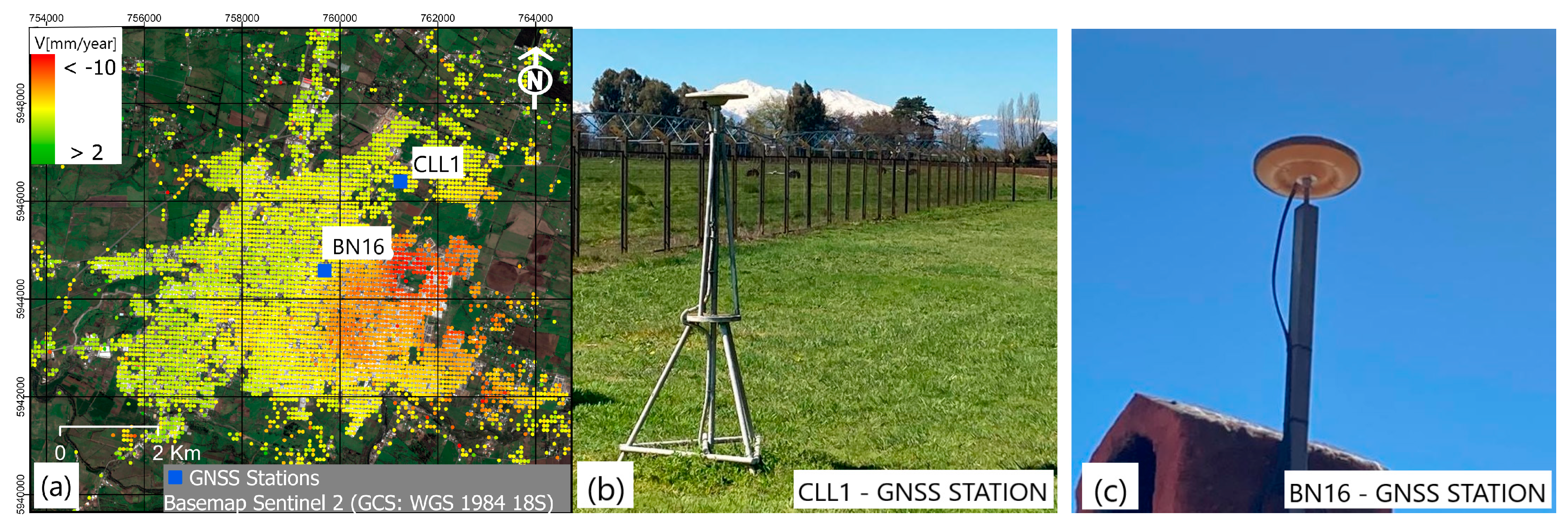
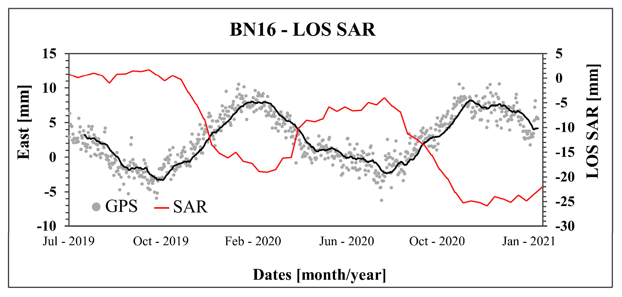
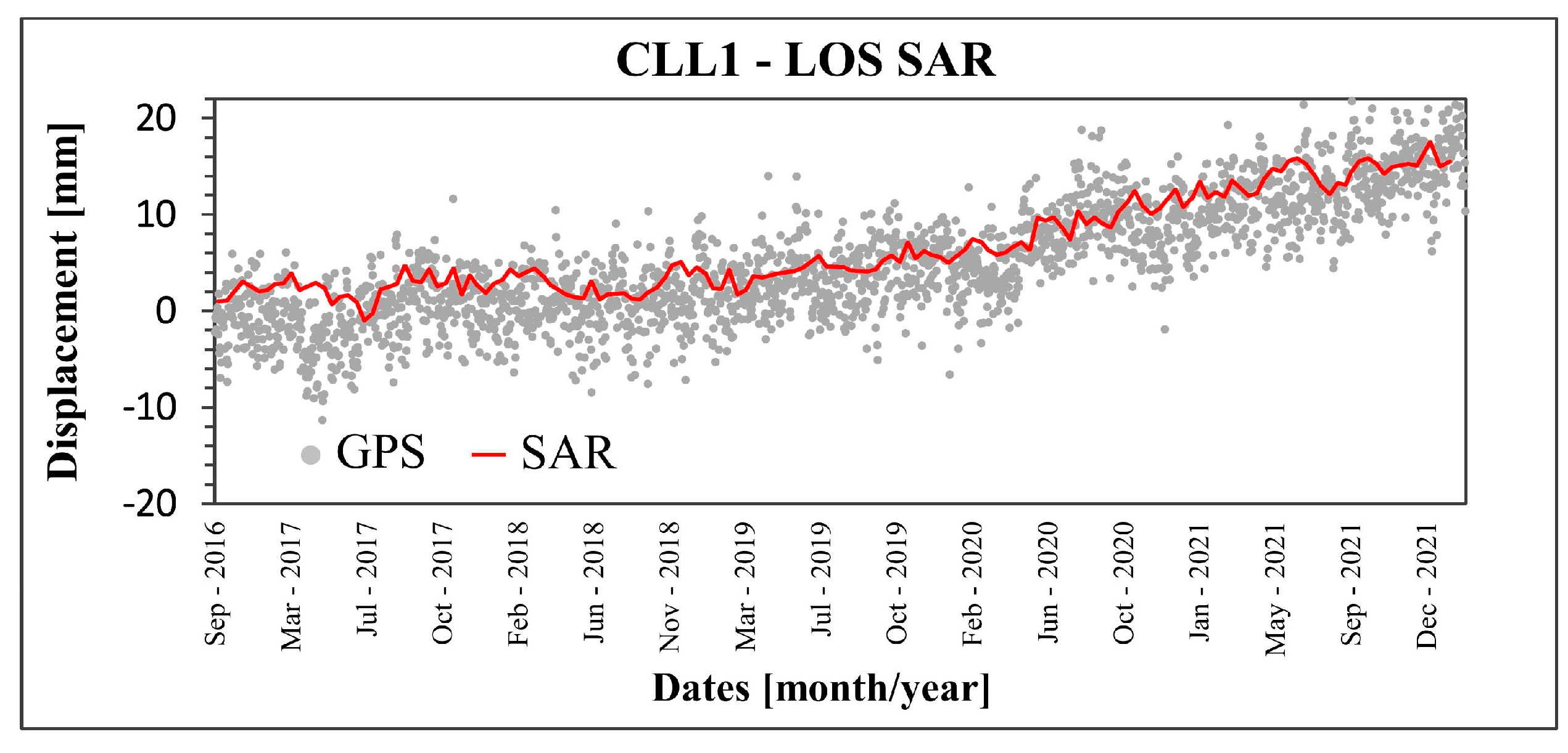
InSAR Measurement Verification

The SAR measurements were validated by comparing the time series of the continuous GNSS stations available in the study area. GPS accuracy, unlike InSAR, has 3D offset fields; however, in our case, East and LOS components were used. GPS data were obtained from an open access resource and accumulated surface displacements at GPS stations were obtained from daily solutions processed at the Nevada Geodetic Laboratory (NGL) of the University of Nevada, Reno, NV, USA [51]. The NGL also routinely updates the data for stations moving in a global reference frame. The time series of the P-SBAS algorithm has been successfully compared and validated in previous studies [18,39]. The reliability of the results was verified through the correlation of time series using InSAR with GPS measurements. The location of the GPS devices is generally in stable soils; in our this case, BN16 is located in the deformation area and CLL1 is located outside the deformation area (see Figure 4a). The GNSS stations used, BNL16 and CLL1, are shown in Figure 4b,c, respectively.
Below presents the comparisons between both independent signals plotted in the GPS InSAR and BN16 time series. Comparing the LOS SAR and the East component of the BN16, we observed a deformation with a seasonal trend for the recorded period 2019–2021; GPS recording began in 2019. For the winter periods, the SAR measurements registered an uplift and west displacement for GPS. On the contrary, in the summer period, the SAR measurements registered subsidence and east displacement for GPS (see Figure 5).
As a second verification, a projection of the GPS CLL1 has been made using the unit vectors of LOS SAR, which are the directional cosines (E), (N), and (U). According to the results, for both signals there was a minor uplift of 15 mm in a 6-year period caused by tectonic influence due to the location of the study area in the Chilean subduction zone. It follows that the results obtained for both GPS-SAR signals show common displacement trends (see Figure 6), which implies reliable successive analysis.

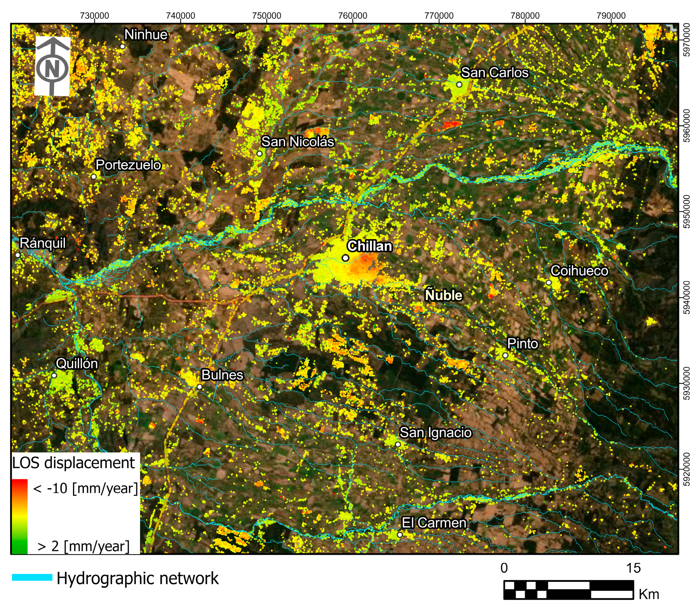
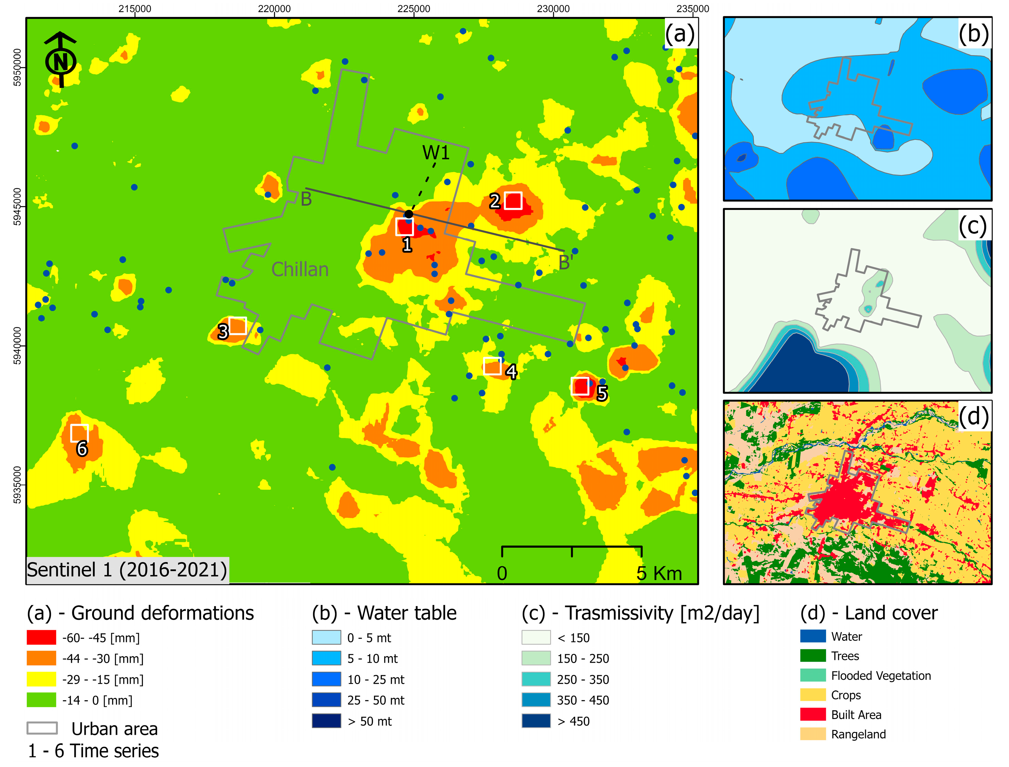
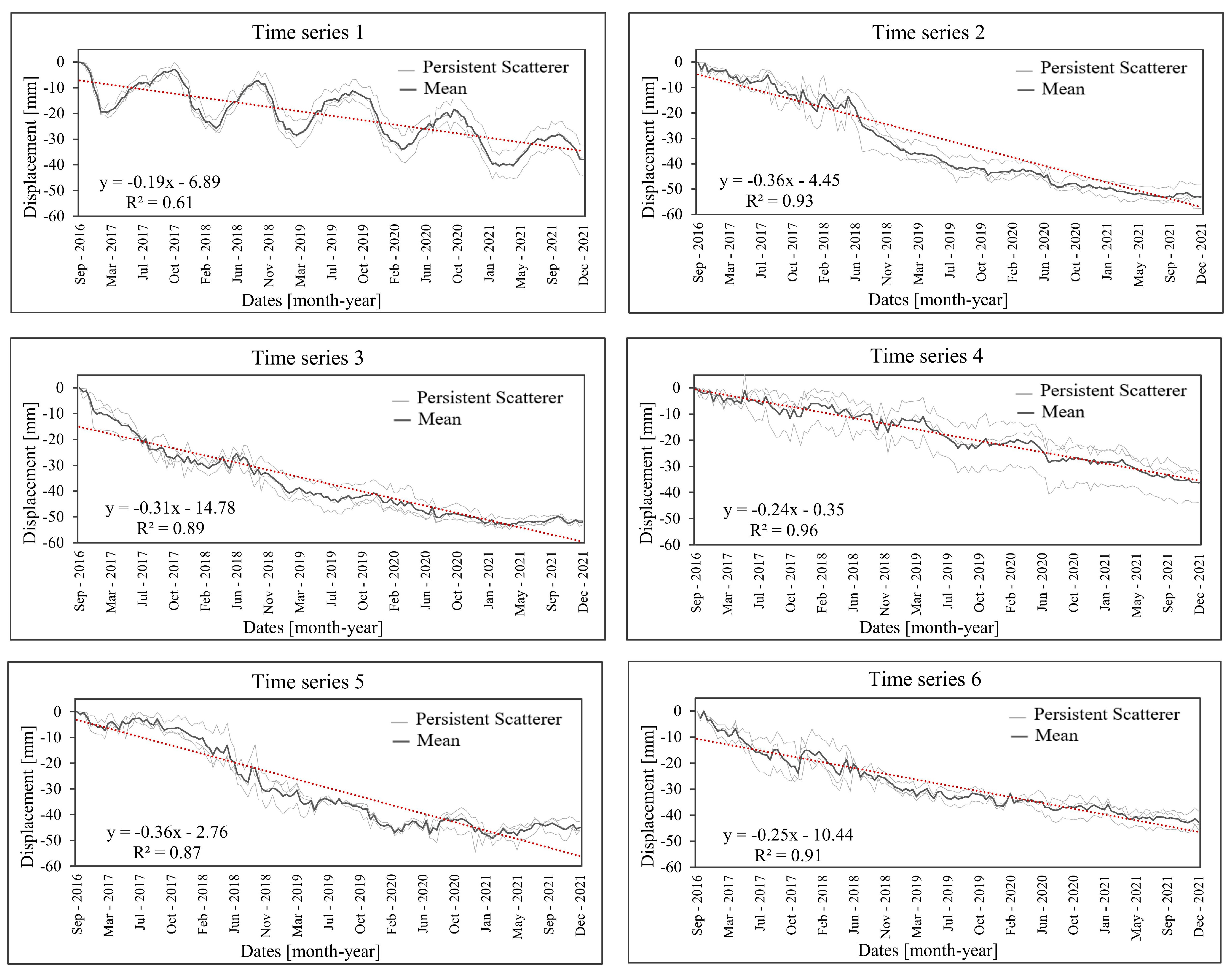
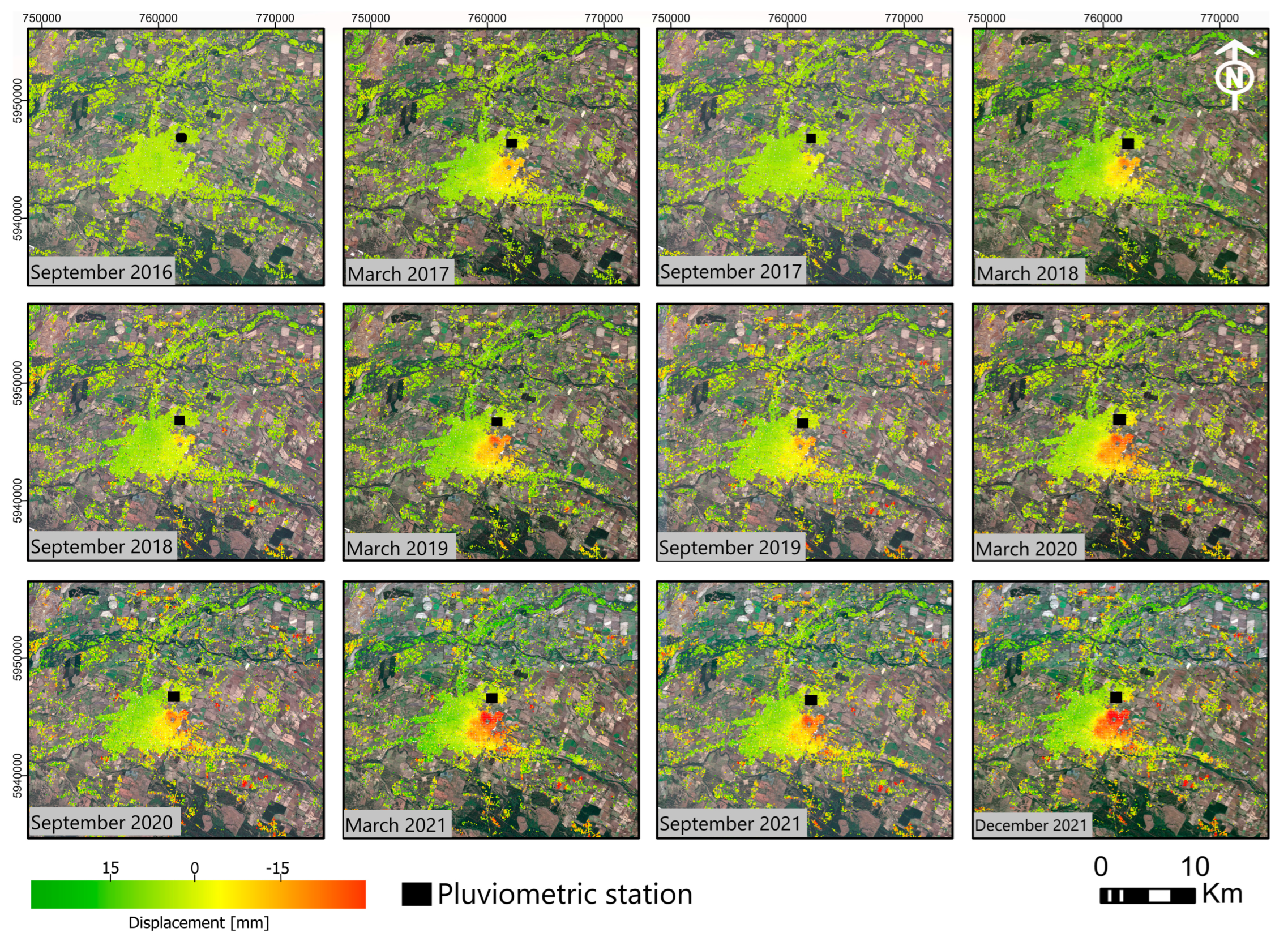
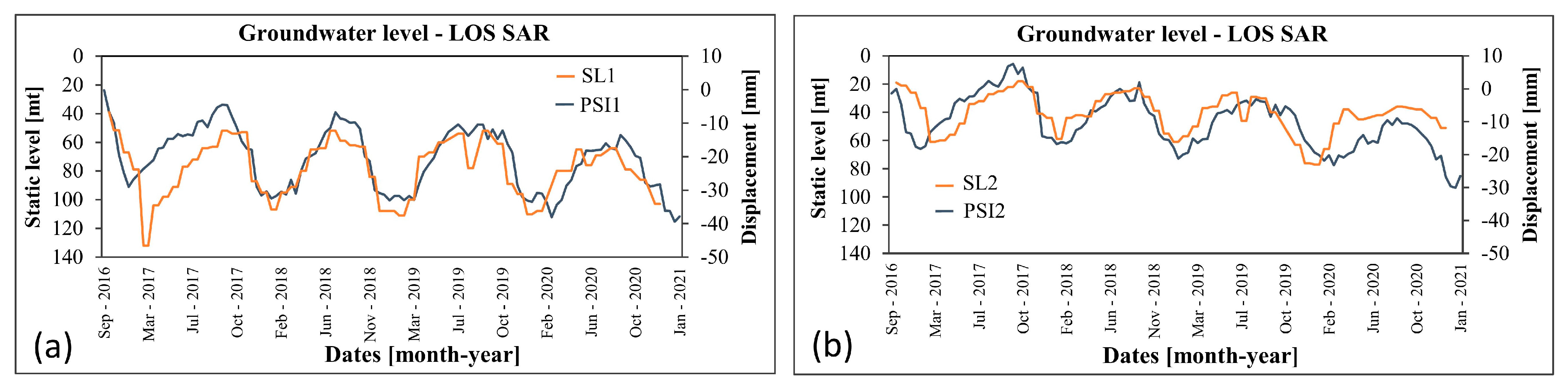
4.2. Ground Deformation and Time-Series

The InSAR results provided a total of 15,543 PSI targets for the study area. This made it possible to estimate the continuous deformation in the entire extension of the area and the compressible thicknesses. To achieve this, the kriging geostatistical interpolation tool [52] was used, where the cumulative displacement in mm was classified for the satellite surveillance period 2016–2021 (see Figure 7a). The main source of natural recharge of the aquifer system corresponds to rain infiltration, which is estimated at 209.82 mm per year and is equivalent to a volume of 116.94 Hm3, with an estimated natural infiltration time of approximately one month for areas where the piezometric level does not exceed 20 m depth (see Figure 7b). The calculation and zoning of the transmissivity in the study area indicate that the most favorable hydraulic conditions are found in the N-E sector of the city of Chillan. This sector has an elongation with a NW-SE direction and has a transmissibility range between 100 and 240 m2/day. The values indicate a deformation rate of up to 60 mm near the Chillan area, and other anomalous deformations in areas where the extraction wells are located. Based on the study conducted by F. Avilés [44], for the Chillan area, we can observe that the transmissivity varies between 150 and 450 m2/day (see Figure 7c). In addition, it is known that soil cover can have profound effects on aquifer recharge processes and soil types, and vegetation densities can influence evapotranspiration patterns. In this case, a large number of crops are observed that influence the dynamics of the aquifer (see Figure 7d).
The main cause of ground deformation may be due to the intensive pumping carried out by the Sanitary company to supply drinking water to the city of Chillan, which is concentrated in a confined aquifer located between 100 and 250 m deep. By concentrating the pumping between several wells, an area is produced where the hydraulic pressure within the aquifer decreases, which translates into a reduction in the bearing capacity of the soil, generating a subsidence process, with deformations of up to 60 mm, which affects the city of Chillan and its surroundings.
To determine aquifer deterioration and its relation to changes in piezometric levels, it is vital to understand the temporal evolution. In this sense, InSAR offers the possibility of obtaining the time series of displacements with a temporal resolution that goes from 6 to 12 days of Sentinel 1 by providing the deformation history of each of the 145 SAR images between September 2016 and December 2021, which is essential to study the kinematics of a certain phenomenon caused by groundwater withdrawal.
The time series were carried out in the deformation area; for this we selected three PSI targets contained in six cells of 100 × 100 m each and numbered from 1 to 6 (white box), as shown in Figure 7a. The time series shown in Figure 8 evidence the variations in the PSI target and the mean calculated for each PSI contained in the cell, indicated in the color blue. According to the results of the time series, there is a very good fit between the PSI measurements of the cell, indicated as mean; in addition, R2 determines the dynamic evolution of groundwater and soil compaction.
Time series 1 shows very pronounced seasonal values, influenced by the extraction of water in the wells close to cell 1, which reach extraction flow rates of 80 l/s for well 1 (W1). This type of behavior responds to the concatenation of periods of depletion, followed by a period of recovery of the aquifer. This response is usually associated with small seasonal variations correlated with the time of year and in aquifers with high elastic mechanical behavior [54]. In some cases, this behavior can also be observed in areas that are affected by strategic pumping in times of drought if the elastic component is high [55].
Time series 2–6 indicate less accentuated seasonal values and a tendency to subsidence, reaching deformation values of up to 60 mm in a 6-year period; this situation possibly responds to a continuous decrease in piezometric levels [25,31,56].

4.3. Spatial and Temporal Variations

In this section, we explore the main factor that causes the deformation of the surface due to the extraction of groundwater and investigate the spatial relationship between the seasonal variation in the water table and ground surface deformation. For this, we sought to estimate the variability of the water table from the winter–summer surface deformations by considering the accumulated seasonal displacements in millimeter units.
To determine the seasonal variations, the temporal and spatial evolution is mapped, with the winter (September) and the summer maps (March) shown in Figure 9. This principle applies when it is required to know an equivalent behavior of variability of the water table in basins or specific areas using PSI measurements. Starting from the temporary record, it can be observed for September 2016 that the signal indicates a cumulative displacement close to 0, while in the last record of December 2021, the subsidence is evident and reaches values of up to 60 mm of cumulative displacement. It is confirmed that the subsidence increases gradually in the summer periods, where there is an evident deterioration of the aquifer; on the contrary, in the winter periods, there is a recovery, procured by precipitations and the increase in snowfall in the Andes mountain range.
The fluctuation of the water table depends on the amount, distribution, and frequency of rainfall. For this reason, it was necessary to register the records of precipitation at the meteorological station of the University of Concepción between the period September 2016 and December 2021. These were compared with the displacements of the earth’s surface detected by the SAR sensor using the PSI target with the greatest displacement of the deformation area (see Figure 10), evidencing a high correlation in the seasonal variation for winter (July–August–September) and summer (January–February–March).
Determining the spatial influence of water withdrawals is one of the most useful results for aquifer surveillance. Since the aquifers are tapped through a large number of wells, they amplify each other to create a deformed area. Extractions of water through pumping wells generate a cone of depression in the aquifer that is reflected on the surface as subsidence [57]. Therefore, the deformed area of 8.25 “km2” is identified in red, with the number of wells and their respective flow (see Figure 11). The deformed area is affected by seasonal fluctuations in the aquifer that are altered by variations in well production, rainfall, and sediment type. In the deformation area, the flow rates of the wells varied during the analyzed period, with increased and decreased in production between 40 and 80 l/s, acquired both in height and depth.
InSAR technologies have achieved significant improvements in spatial and temporal resolution. The precision of the measurements are useful resources for the monitoring and management of water resources storage. The piezometric measurement can only be carried out in a timely manner, without continuous data, with a low density of control points; however, InSAR technology, due to its good spatial density of PSI targets, makes it possible to observe the depressions on the surface and correlate them with the groundwater dynamics. To demonstrate the fluctuation of the deformation area, we have selected Well 1 (W1) and Well 2 (W2) to the northeast and southeast, respectively, where the seasonal deformation of the sediments in PSI 1 and PSI 2 is shown, and the static level (SL1) and (SL2) show synchronized variations (see Figure 12). This phenomenon occurs throughout the deformation area and is accentuated in the area near the wells. In addition, a decrease in the recovery capacity of the aquifer is evidenced, dominated by the elastic deformation of the sediments.

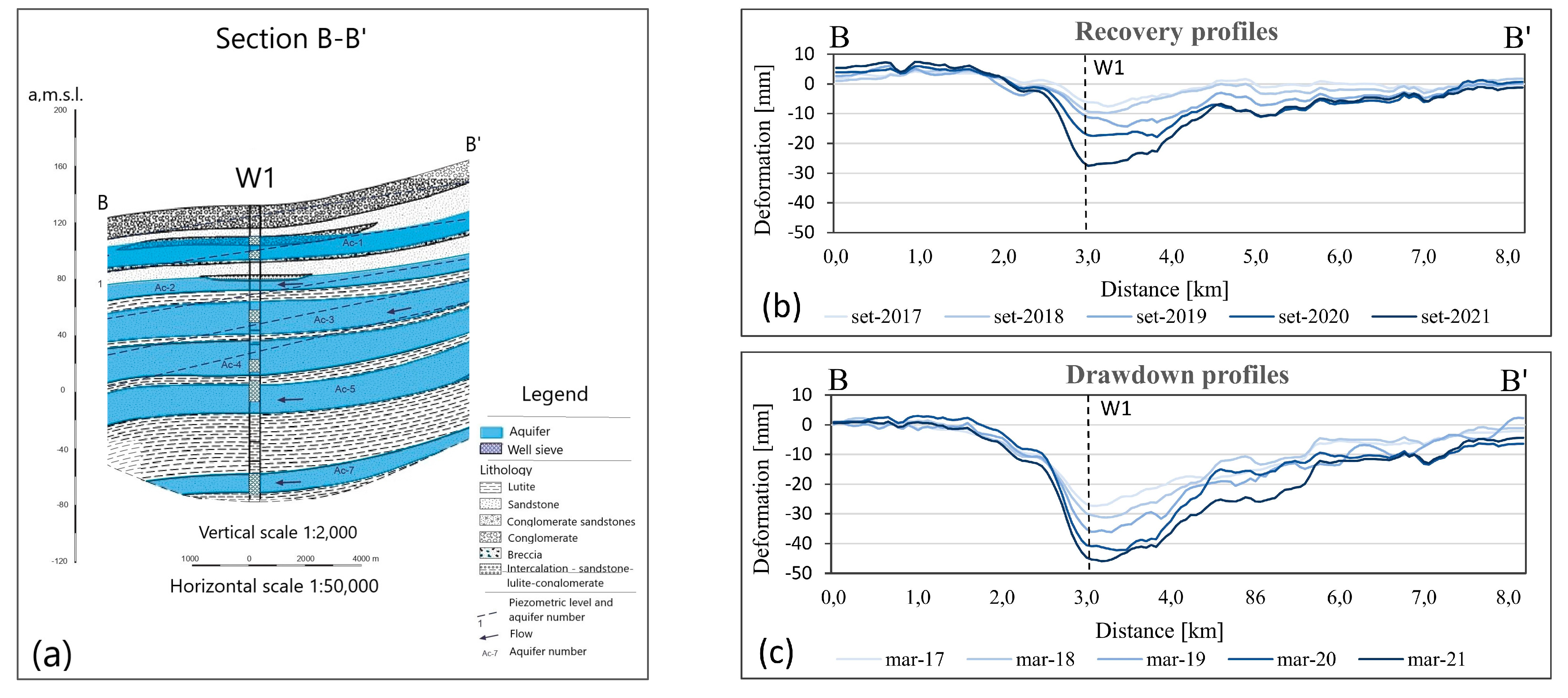
4.4. Geological and Hydrogeological Interpretations

The hydrogeological structure and soil types that make up an aquifer are primarily responsible for the dynamics and changes in piezometric levels. The aquifers located in the study area are detrital aquifers composed of complex combinations of sediments of different particle sizes and hydraulic properties. The most productive parts are made up of coarse sediments and have a more elastic behavior, typical of coarser sediments (sand and gravel). The areas of fine sediments (sandstones and silts) act as aquitards and are scarcely exploited due to their low transmissivities. When these layers desaturate, they begin to transfer water to the underlying areas, producing a compaction of the materials (subsidence). Therefore, elastoplastic deformation is produced that is only partially recovered in later times when the extractions stop and the piezometric levels are recovered. This leaves a permanent LOS deformation that can be captured by InSAR signals. Inelastic subsidence is of concern from both the structural and management points of view of the aquifer, since the total storage capacity may be reduced due to the reorganization of the sediment structure under pressure change [58].
The main factors that control storage are compression ratio and effective stress and direct and inverse dependency. Effective stress increases with depth, so larger effects are expected in shallow aquifers [28]. According to the elastic pore model developed by Terzaghi, K. [59] and Biot, M. [60], the effective stress variation is related to the changes in the hydraulic head (Δh) of the sediment, so if there is a change in a given stress field, caused in this case by a change in pore pressure (Δu), it will result in a deformation of the surface. For aquifer systems, the steady decrease in Δh at piezometers suggests that, at those sites, the heads fall further and further below consolidation, thus overcoming pre-consolidation stress and causing irreversible deformation of the aquifer system [61]. Therefore, InSAR-derived compaction, which is the trend in the time series (e.g., Figure 8), reflects the inelastic components and provides a lower bound on the magnitude of subsidence. In addition, the compression index depends on the granulometry of the soil; fine soils (i.e., Lutite and Sandstone) have higher compression, while coarse and more rigid soils (i.e., Breccia and Conglomerate) have lower compression values. Details of the structure are shown in Figure 13a.
The variation in the water table allows to determine with greater precision the hydrogeological behavior of what happens in the area of interest, being one of the most important inputs in the analysis of unstable areas [58]. The knowledge of the spatial distribution of the finer sediments prone to compaction is important for the interpretation of the surface deformation results obtained with InSAR. In this sense, the hydrogeological data obtained in F. Aviles [44], mostly through research boreholes and the drilling witnesses of some of the wells, are the best information that is usually available. It is important to relate aquifer deformation to hydrogeological factors, so we have extracted a detail from the hydrogeological section, a B-B″ profile over the deformation zone (see Figure 13a).
Subsequently, the seasonal deformation has been estimated for the recovery periods in September (winter), as shown in Figure 13b, and the depletion times in March (summer), shown in Figure 13c. In both cases the depression of the aquifer is evidenced in the period observed with InSAR (2016–2021), in section B-B, Well 1 (W1) is identified with the coordinates 36°36′19″ Sud latitude 72°4′36″ West longitude and an extraction of 80 l/s, located in the urban center of the city of Chillan.
It is also taken into account that there are causes induced by the viscoelastic behavior of the materials and the appearance of a softening and loss of rigidity of the materials with the passage of time. These causes are not so directly related to the evolution of the piezometric levels and require more in-depth analysis to confirm them. All the information that has been obtained in this study can be used to carry out successive numerical and geo-mechanical models for aquifer deterioration trends.

5. Conclusions

InSAR technology is very advanced. In this particular study, it has been shown that the precision of the measurements can support decision makers for a timely management of groundwater storage, water resources management, and to mitigate potential hazards. The detection of subsidence has allowed us to determine the most vulnerable areas; in addition, the hydrogeological frameworks have allowed us to obtain a better understanding of the phenomenon. However, there is a challenge for the development of forecast models of aquifer confinement and groundwater flow dynamics that complement numerical modeling and geo-mechanical models.
By considering the InSAR technique and the in situ data, the displacements of the earth’s surface are confirmed as a consequence of the extraction of groundwater. It was possible to detect the impact of pumping from the wells used for the drinking water supply in an urban area with high water demand, demonstrating the possibilities of this method to quickly measure environmental impacts associated with intensive groundwater withdrawals. InSAR has proven useful in recording deformations and variations in aquifers and allowing us to investigate seasonal variations in groundwater. The flexibility of the information obtained from InSAR allows for the efficient organization and distribution of information in GIS. This could contribute significantly to public and private institutions in regard to environmental surveillance, allowing them to identify and communicate an alert situation and enabling them to respond and act appropriately in the event of overexploitation of water, reducing the irreversible deterioration of aquifers.
InSAR early warning surveillance has been shown to be an efficient and low-cost technology that can be used for correct water management and sustainability. There is a high correlation between the measurements of ground deformation registered with InSAR and static levels; this is key for the management of groundwater storage and relevant to groundwater resource exploration and associated groundwater-induced hazards such as land subsidence. The large amount of open SAR data available has made it possible to create a high-frequency updated time series, obtaining very reliable results. The use of an algorithm based on parallel computing has reduced processing times, which in many cases is a very complex routine. SAR sensor results were displayed similarly to continuous GNSS stations. Despite the orbital angle of incidence, we consider that both technologies are complementary. However, InSAR allowed us to have greater spatial coverage, which is key to determining the areas of aquifer deterioration.

Supplementary Materials

The following supporting information can be downloaded at: https://www.mdpi.com/article/10.3390/rs15071786/s1, Supplementary Materials provide LOS displacement map of study area in .kmz file, in addition, GNSS time series from BN16 and CLL1 stations, in .txt and .png files.

Author Contributions

Conceptualization, F.O., D.R., G.M. and J.L.A.; methodology, F.O., D.R., G.M. and J.L.A.; SAR data processing, F.O.; validation F.O.; writing F.O., D.R., G.M. and J.L.A.; supervision, G.M. and J.L.A. All authors have read and agreed to the published version of the manuscript.

Funding

Financial supported by CRHIAM, Center for Research on Water for Agriculture and Mining (ANID/FONDAP/15130015).

Data Availability Statement

DGA provides the location of the registered wells at the area directly through their internet web page and the Chilean Superintendency of Sanitary Services (SISS) provides pumping data of the well upon request by Transparency Law. Hydrogeological information such as maps and stratigraphic profiles, from F. Aviles’ [44], available at the Department of Water Resources of the University of Concepcion, Chile, as layer formats (Shapefile). Digital Elevation Model (DEM), is georeferenced in WGS84—UTM Zone 18S, provided by the Chilean National Geoportal IDE https://www.ide.cl/ (accessed on 15 March 2022).

Acknowledgments

To the CRHIAM Water Research Center for Agriculture and Mining (ANID/FONDAP/15130015). F.O. acknowledgments the operational support of Geohazard TEP and Terradue.

Conflicts of Interest

The authors declare no conflict of interest.

References

  1. Wang, H.-W.; Lin, C.-W.; Yang, C.-Y.; Ding, C.-F.; Hwung, H.-H.; Hsiao, S.-C. Assessment of Land Subsidence and Climate Change Impacts on Inundation Hazard in Southwestern Taiwan. Irrig. Drain. 2018, 67, 26–37. [Google Scholar] [CrossRef]
  2. Dinar, A.; Esteban, E.; Calvo, E.; Herrera, G.; Teatini, P.; Tomás, R.; Li, Y.; Ezquerro, P.; Albiac, J. We lose ground: Global assessment of land subsidence impact extent. Sci. Total Environ. 2021, 786, 147415. [Google Scholar] [CrossRef] [PubMed]
  3. Minderhoud, P.S.J.; Erkens, G.; Pham, V.H.; Bui, V.T.; Erban, L.; Kooi, H.; Stouthamer, E. Impacts of 25 years of groundwater extraction on subsidence in the Mekong delta, Vietnam. Environ. Res. Lett. 2017, 12, 064006. [Google Scholar] [CrossRef] [PubMed]
  4. Ferreira, C.S.; Seifollahi-Aghmiuni, S.; Destouni, G.; Ghajarnia, N.; Kalantari, Z. Soil degradation in the European Mediterranean region: Processes, status and consequences. Sci. Total Environ. 2022, 805, 150106. [Google Scholar] [CrossRef]
  5. Li, H.; Zhu, L.; Dai, Z.; Gong, H.; Guo, T.; Guo, G.; Wang, J.; Teatini, P. Spatiotemporal modeling of land subsidence using a geographically weighted deep learning method based on PS-InSAR. Sci. Total Environ. 2021, 799, 149244. [Google Scholar] [CrossRef] [PubMed]
  6. Smith, R.G.; Majumdar, S. Groundwater Storage Loss Associated with Land Subsidence in Western US Mapped Using Machine Learning. Water Resour. Res. 2020, 56, e2019WR026621. [Google Scholar] [CrossRef]
  7. Liu, R.; Zhao, Y.; Cao, G.; Wang, Q.; Ma, M.; Li, E.; Deng, H. Threat of land subsidence to the groundwater supply capacity of a multi-layer aquifer system. J. Hydrol. Reg. Stud. 2022, 44, 101240. [Google Scholar] [CrossRef]
  8. Abidin, H.Z.; Andreas, H.; Gumilar, I.; Sidiq, T.P.; Gamal, M. Environmental impacts of land subsidence in urban areas of Indonesia. In FIG Working Week; TS 3—Positioning and Measurement: Sofia, Bulgaria, 2015; pp. 1–12. [Google Scholar]
  9. Wu, W.Y.; Lo, M.H.; Wada, Y.; Famiglietti, J.S.; Reager, J.T.; Yeh, P.J.F.; Ducharne, A.; Yang, Z.L. Divergent effects of climate change on future groundwater availability in key mid-latitude aquifers. Nat. Commun. 2020, 11, 3710. [Google Scholar] [CrossRef]
  10. La Vigna, F. Review: Urban groundwater issues and resource management, and their roles in the resilience of cities. Hydrogeol. J. 2022, 30, 1657–1683. [Google Scholar] [CrossRef]
  11. Guzy, A.; Malinowska, A.A. State of the Art and Recent Advancements in the Modelling of Land Subsidence Induced by Groundwater Withdrawal. Water 2020, 12, 2051. [Google Scholar] [CrossRef]
  12. Ceccatelli, M.; Del Soldato, M.; Solari, L.; Fanti, R.; Mannori, G.; Castelli, F. Numerical modelling of land subsidence related to groundwater withdrawal in the Firenze-Prato-Pistoia basin (central Italy). Hydrogeol. J. 2021, 29, 629–649. [Google Scholar] [CrossRef]
  13. Galloway, D.L.; Burbey, T.J. Review: Regional Land Subsidence Accompanying Groundwater Extraction. Hydrogeol. J. 2011, 19, 1459–1486. [Google Scholar] [CrossRef]
  14. Arangio, S.; Bontempi, F.; Ciampoli, M. Structural integrity monitoring for dependability. Struct. Infrastruct. Eng. 2011, 71, 75–86. [Google Scholar] [CrossRef]
  15. Crosetto, M.; Monserrat, O.; Cuevas, M.; Crippa, B. Spaceborne Differential SAR Interferometry: Data Analysis Tools for Deformation Measurement. Remote Sens. 2011, 3, 305–318. [Google Scholar] [CrossRef] [Green Version]
  16. Manunta, M.; Marsella, M.; Zeni, G.; Sciotti, M.; Atzori, S.; Lanari, R. Two-scale surface deformation analysis using the SBAS-DInSAR technique: A case study of the city of Rome, Italy. Int. J. Remote Sens. 2008, 29, 1665–1684. [Google Scholar] [CrossRef]
  17. Bozzano, F.; Esposito, C.; Mazzanti, P.; Patti, M.; Scancella, S. Imaging Multi-Age Construction Settlement Behaviour by Advanced SAR Interferometry. Remote Sens. 2018, 10, 1137. [Google Scholar] [CrossRef] [Green Version]
  18. Orellana, F.; Hormazábal, J.; Montalva, G.; Moreno, M. Measuring Coastal Subsidence after Recent Earthquakes in Chile Central Using SAR Interferometry and GNSS Data. Remote Sens. 2022, 14, 1611. [Google Scholar] [CrossRef]
  19. Foumelis, M.; Papageorgiou, E.; Stamatopoulos, C. Episodic ground deformation signals in Thessaly Plain (Greece) revealed by data mining of SAR interferometry time series. Int. J. Remote Sens. 2016, 37, 3696–3711. [Google Scholar] [CrossRef]
  20. Sun, Q.; Zhang, L.; Ding, X.L.; Hu, J.; Li, Z.W.; Zhu, J.J. Slope deformation prior to Zhouqu, China landslide from InSAR time series analysis. Remote Sens. Environ. 2015, 156, 45–57. [Google Scholar] [CrossRef]
  21. Brunori, C.A.; Norini, G.; Stramondo, S.; Capra, L.; Zucca, F.; Groppelli, G.; Bignami, C.; Chini, M.; Manea, M.; Manea, V. Crustal deformation induced by volcanic activity measured by InSAR time series analysis (Volcan de Colima-Mexico). In EGU General Assembly Conference Abstracts; 2010; p. 6958. Available online: https://ui.adsabs.harvard.edu/abs/2010EGUGA..12.6958B/abstract (accessed on 1 January 2022).
  22. Orellana, F.; Delgado Blasco, J.M.; Foumelis, M.; D’Aranno, P.J.V.; Marsella, M.A.; Di Mascio, P.D. Dinsar for road infrastructure monitoring: Case study highway network of Rome metropolitan (Italy). Remote Sens. 2020, 12, 3697. [Google Scholar] [CrossRef]
  23. Infante, D.; Di Martire, D.; Confuorto, P.; Tessitore, S.; Ramondini, M.; Calcaterra, D. Differential Sar Interferometry Technique for Control of Linear Infrastructures Affected by Ground Instability Phenomena. ISPRS Int. Arch. Photogramm. Remote Sens. Spat. Inf. Sci. 2018, 3, 251–258. [Google Scholar] [CrossRef] [Green Version]
  24. Cigna, F.; Tapete, D. Urban growth and land subsidence: Multi-decadal investigation using human settlement data and satellite InSAR in Morelia, Mexico. Sci. Total Environ. 2022, 811, 152211. [Google Scholar] [CrossRef] [PubMed]
  25. Ezquerro, P.; Tomás, R.; Béjar-Pizarro, M.; Fernández-Merodo, J.A.; Guardiola-Albert, C.; Staller, A.; Sánchez-Sobrino, J.A.; Herrera, G. Improving multi-technique monitoring using Sentinel-1 and Cosmo-SkyMed data and upgrading groundwater model capabilities. Sci. Total Environ. 2020, 703, 134757. [Google Scholar] [CrossRef] [PubMed] [Green Version]
  26. Chen, B.; Gong, H.; Chen, Y.; Li, X.; Zhou, C.; Lei, K.; Zhu, L.; Duan, L.; Zhao, X. Land subsidence and its relation with groundwater aquifers in Beijing Plain of China. Sci. Total Environ. 2020, 735, 139111. [Google Scholar] [CrossRef] [PubMed]
  27. Awasthi, S.; Jain, K.; Bhattacharjee, S.; Gupta, V.; Varade, D.; Singh, H.; Narayan, A.B.; Budillon, A. Analyzing urbanization induced groundwater stress and land deformation using time-series Sentinel-1 datasets applying PSInSAR approach. Sci. Total Environ. 2022, 844, 157103. [Google Scholar] [CrossRef]
  28. Orellana, F.; Moreno, M.; Yáñez, G. High-Resolution Deformation Monitoring from DInSAR: Implications for Geohazards and Ground Stability in the Metropolitan Area of Santiago, Chile. Remote Sens. 2022, 14, 6115. [Google Scholar] [CrossRef]
  29. Amitrano, D.; Di Martino, G.; Iodice, A.; Mitidieri, F.; Papa, M.N.; Riccio, D.; Ruello, G. Sentinel-1 for Monitoring Reservoirs: A Performance Analysis. Remote Sens. 2014, 6, 10676–10693. [Google Scholar] [CrossRef] [Green Version]
  30. Bozzano, F.; Esposito, C.; Franchi, S.; Mazzanti, P.; Perissin, D.; Rocca, A.; Romano, E. Understanding the Subsidence Process of a Quaternary Plain by Combining Geological and Hydrogeological Modelling with Satellite InSAR Data: The Acque Albule Plain Case Study. Remote Sens. Environ. 2015, 168, 219–238. [Google Scholar] [CrossRef]
  31. Ezquerro, P.; Herrera, G.; Marchamalo, M.; Tomás, R.; Béjar-Pizarro, M.; Martínez, R. A Quasi-Elastic Aquifer Deformational Behavior: Madrid Aquifer Case Study. J. Hydrol. 2014, 519, 1192–1204. [Google Scholar] [CrossRef] [Green Version]
  32. Ezquerro, P.; Guardiola-Albert, C.; Herrera, G.; Fernández-Merodo, J.A.; Béjar-Pizarro, M.; Bonì, R. Groundwater and Subsidence Modeling Combining Geological and Multi-Satellite SAR Data over the Alto Guadalentín Aquifer (SE Spain). Geofluids 2017, 2017, 1359325. [Google Scholar] [CrossRef]
  33. Ferretti, A.; Prati, C.; Rocca, F. Permanent scatterers in SAR interferometry. IEEE Trans. Geosci. Remote Sens. 2001, 39, 8–20. [Google Scholar] [CrossRef]
  34. Berardino, P.; Fornaro, G.; Lanari, R.; Sansosti, E. A new algorithm for surface deformation monitoring based on small baseline differential SAR interferograms. IEEE Trans. Geosci. Remote Sens. 2002, 40, 2375–2383. [Google Scholar] [CrossRef] [Green Version]
  35. Crosetto, M.; Monserrat, O.; Cuevas-González, M.; Devanthéry, N.; Crippa, B. Persistent Scatterer Interferometry: A Review. ISPRS J. Photogramm. Remote Sens. 2016, 115, 78–89. [Google Scholar] [CrossRef] [Green Version]
  36. Ferretti, A.; Fumagalli, A.; Novali, F.; Prati, C.; Rocca, F.; Rucci, A. A New Algorithm for Processing Interferometric Data-Stacks: SqueeSAR. IEEE Trans. Geosci. Remote Sens. 2011, 49, 3460–3470. [Google Scholar] [CrossRef]
  37. Hooper, A.J. A Multi-Temporal InSAR Method Incorporating Both Persistent Scatterer and Small Baseline Approaches. Geophys. Res. Lett. 2008, 35. [Google Scholar] [CrossRef] [Green Version]
  38. Casu, F.; Elefante, E.; Imperatore, P.; Zinno, I.; Manunta, M.; De Luca, C.; Lanari, R. SBAS-DInSAR Parallel Processing for Deformation Time Series Computation. IEEE J. Sel. Top. Appl. Earth Obs. Remote Sens. 2014, 7, 3285–3296. [Google Scholar] [CrossRef]
  39. Manunta, M.; De Luca, C.; Zinno, I.; Casu, F.; Manzo, M.; Bonano, M.; Fusco, A.; Pepe, A.; Onorato, G.; Berardino, P.; et al. The Parallel SBAS Approach for Sentinel-1 Interferometric Wide Swath Deformation Time-Series Generation: Algorithm Description and Products Quality Assessment. IEEE Trans. Geosci. Remote Sens. 2019, 57, 6259–6281. [Google Scholar] [CrossRef]
  40. Manunta, M.; Casu, F.; Zinno, I.; de Luca, C.; Pacini, F.; Brito, F.; Blanco, P.; Iglesias, R.; Lopez, A.; Briole, P.; et al. The Geohazards Exploitation Platform: An advanced cloud-based environment for the Earth Science community. In Proceedings of the19th EGU General Assembly, EGU2017, Vienna, Austria, 23–28 April 2017; p. 14911. [Google Scholar]
  41. Foumelis, M.; Papadopoulou, T.; Bally, P.; Pacini, F.; Provost, F.; Patruno, J. Monitoring Geohazards Using On-Demand and Systematic Services on Esa’s Geohazards Exploitation Platform. In Proceedings of the IGARSS 2019, IEEE International Geoscience and Remote Sensing Symposium, Yokohama, Japan, 28 July–2 August 2019; IEEE: Piscataway, NJ, USA, 2019; pp. 5457–5460. [Google Scholar] [CrossRef]
  42. Galve, J.P.; Pérez-Peña, J.V.; Azañón, J.M.; Closon, D.; Calò, F.; Reyes-Carmona, C.; Jabaloy, A.; Ruano, P.; Mateos, R.M.; Notti, D.; et al. Evaluation of the SBAS InSAR Service of the European Space Agency’s Geohazard Exploitation Platform (GEP). Remote Sens. 2017, 9, 1291. [Google Scholar] [CrossRef] [Green Version]
  43. Reyes-Carmona, C.; Galve, J.P.; Barra, A.; Monserrat, O.; Maria Mateos, R.; Azañón, J.M.; Perez-Pena, J.V.; Ruano, P. The Sentinel-1 CNR-IREA SBAS service of the European Space Agency’s Geohazard Exploitation Platform (GEP) as a powerful tool for landslide activity detection and monitoring. In Proceedings of the EGU General Assembly, Vienna, Austria, 3–8 May 2020; p. 19410. [Google Scholar] [CrossRef]
  44. Avilés, F. Hydrogeological characterization of the Chillán sheet (36°30′–36°45′South Latitude and 72°00′–72°15′ West Longitude), VIII Region of Bíobío, Chile; Report to qualify for the title of Geologist; University of Concepción: Concepcion, Chile, 2006. [Google Scholar]
  45. Zinno, I.; Casu, F.; De Luca, C.; Elefante, S.; Lanari, R.; Manunta, M. A cloud computing solution for the efficient implementation of the P-SBAS DInSAR approach. IEEE J. Sel. Top. Appl. Earth Obs. Remote Sens. 2016, 10, 802–817. [Google Scholar] [CrossRef]
  46. Imperatore, P.; Pepe, A.; Sansosti, E. High performance computing in satellite SAR interferometry: A critical perspective. Remote Sens. 2021, 13, 4756. [Google Scholar] [CrossRef]
  47. Dong, S.; Samsonov, S.; Yin, H.; Ye, S.; Cao, Y. Time-series analysis of subsidence associated with rapid urbanization in Shanghai, China measured with SBAS InSAR method. Environ. Earth Sci. 2014, 72, 677–691. [Google Scholar] [CrossRef]
  48. Farr, T.G.; Rosen, P.A.; Caro, E.; Crippen, R.; Duren, R.; Hensley, S.; Kobrick, M.; Paller, M.; Rodriguez, E.; Roth, L.; et al. The Shuttle Radar Topography Mission. Rev. Geophys. 2007, 45, RG2004. [Google Scholar] [CrossRef] [Green Version]
  49. Yague-Martinez, N.; DeZan, F.; Prats-Iraola, P. Coregistration of Interferometric Stacks of Sentinel-1 TOPS Data. IEEE Geosci. Remote Sens. Lett. 2017, 14, 1002–1006. [Google Scholar] [CrossRef] [Green Version]
  50. Arumí, J.L.; Rivera, D.; Muñoz, E.; Billib, M. Interactions between surface and groundwater in the Bío Bío region of Chile. Work. Proj. 2012, 12, 4–13. [Google Scholar]
  51. Blewitt, G.; Hammond, W.C.; Kreemer, C. Harnessing the GPS data explosion for interdisciplinary science. Eos 2018, 99, 485. [Google Scholar] [CrossRef]
  52. Goovaerts, P. Geostatistics for Natural Resources Evaluation; Oxford University Press: Oxford, UK, 1997. [Google Scholar] [CrossRef]
  53. Brown, C.F.; Brumby, S.P.; Guzder-Williams, B.; Birch, T.; Hyde, S.B.; Mazzariello, J.; Czerwinski, W.; Pasquarella, V.J.; Haertel, R.; Ilyushchenko, S.; et al. Dynamic World, Near real-time global 10 m land use land cover mapping. Sci. Data 2022, 9, 251. [Google Scholar] [CrossRef]
  54. Galloway, D.L.; Hoffmann, J. The application of satellite differential SAR interferometry-derived ground displacements in hydrogeology. Hydrogeol. J. 2006, 15, 133–154. [Google Scholar] [CrossRef] [Green Version]
  55. González, P.J.; Tiampo, K.F.; Palano, M.; Cannavó, F.; Fernández, J. The 2011 Lorca earthquake slip distribution controlled by groundwater crustal unloading. Nat. Geosci. 2012, 5, 821–825. [Google Scholar] [CrossRef] [Green Version]
  56. Bonì, R.; Herrera, G.; Meisina, C.; Notti, D.; Béjar-Pizarro, M.; Zucca, F.; González, P.J.; Palano, M.; Tomás, R.; Fernández, J.; et al. Twenty-year advanced DInSAR analysis of severe land subsidence: The Alto Guadalentín Basin (Spain) case study. Eng. Geol. 2015, 198, 40–52. [Google Scholar] [CrossRef] [Green Version]
  57. Taftazani, R.; Kazama, S.; Takizawa, S. Spatial Analysis of Groundwater Abstraction and Land Subsidence for Planning the Piped Water Supply in Jakarta, Indonesia. Toilet 2022, 14, 3197. [Google Scholar] [CrossRef]
  58. Earle, S. Physical Geology. Victoria, BC: BCcampus. 2015. Available online: https://opentextbc.ca/geology/ (accessed on 21 March 2023).
  59. Terzaghi, K. Principles of soil mechanics: IV. Settlement and consolidation of clay. Erdbaummechanic 1925, 95, 874–878. [Google Scholar]
  60. Biot, M. General theory of three-dimensional consolidation. J. Appl. Phys. 1941, 12, 155–164. [Google Scholar] [CrossRef]
  61. Cigna, F.; Tapete, D. Land Subsidence and Aquifer-System Storage Loss in Central Mexico: A Quasi-Continental Investigation with Sentinel-1 InSAR. Geophys. Res. Lett. 2022, 49, e2022GL098923. [Google Scholar] [CrossRef]
Figure 1. Study area: Chile central valley, Chillan location in Itata basin, background Digital Elevation Model (DEM) ALOS Palsar 30 mt.
Remotesensing 15 01786 g001
Figure 2. (a) Hydrogeological map, and (b) Section A-A’ in the study area, (modified from F. Aviles [44]).
Remotesensing 15 01786 g002
Figure 3. Overall view in study area, distribution of Persistent Scatterers Interferometry (PSI) and LOS displacement map [mm/year], background ESRI maxar source.
Remotesensing 15 01786 g003
Figure 4. (a) Location GNSS stations in the study area, (b) CLL1 GPS, and (c) BNL16 GPS devices.
Remotesensing 15 01786 g004
Figure 5. GPS and SAR time series, for BNL16 station and LOS SAR direction.
Remotesensing 15 01786 g005
Figure 6. GPS and SAR time series, projected along the LOS SAR directions.
Remotesensing 15 01786 g006
Figure 7. (a) Ground deformation map [mm], (b) Water table map (c) Transmissivity map (modified from F. Avilés [44]) and (d) Land cover map, available in dynamic world data (Brown et al. [53]).
Remotesensing 15 01786 g007
Figure 8. InSAR 1–6 time series, from September 2016 to December 2021, from 145 Sentinel 1 acquisitions, gray line represents Persistent Scatterers, and black line the mean.
Remotesensing 15 01786 g008
Figure 9. Seasonal variations map, winter (September) and summer (February–December), background Sentinel 2 image ESA (2022).
Remotesensing 15 01786 g009
Figure 10. Comparison plots of the InSAR time series and monthly rainfall between September 2016–December 2021.
Remotesensing 15 01786 g010
Figure 11. Deformation area and location wells of Sanitary Services Company (ESSBIO), background image Sentinel 2 ESA (2022), yellow dots Well 1 (W1) and Well 2 (W2).
Remotesensing 15 01786 g011
Figure 12. Groundwater level and LOS SAR time series, (a) SL1 and PSI1 for Well 1 (W1), and (b) SL2 and PSI2 for Well 2 (W2).
Remotesensing 15 01786 g012
Figure 13. (a) Details Hydrogeological structure section B-B′ and, (b) Deformation profiles recovery and, (c) Deformation profile drawdown.
Remotesensing 15 01786 g013
Table 1. Features of the Sentinel 1 dataset.
OrbitDescending
SensorSentinel 1B
N° acquisitions145
Date of measurement start10 September 2016
Date of measurement end30 December 2021
Relative orbit156
PolarizationVV
SwathIW-2
Bursts2–3
Disclaimer/Publisher’s Note: The statements, opinions and data contained in all publications are solely those of the individual author(s) and contributor(s) and not of MDPI and/or the editor(s). MDPI and/or the editor(s) disclaim responsibility for any injury to people or property resulting from any ideas, methods, instructions or products referred to in the content.

