Technical Note

Improving Consistency of GNSS-IR Reflector Height Estimates between Different Frequencies Using Multichannel Singular Spectrum Analysis

1
School of Civil Engineering and Architecture, Guangxi University, Nanning 530004, China
2
Chinese Antarctic Center of Surveying and Mapping, Wuhan University, Wuhan 430079, China
3
School of Geomatics Science and Technology, Nanjing Tech University, Nanjing 211816, China
*
Author to whom correspondence should be addressed.
Remote Sens. 2023, 15(7), 1779; https://doi.org/10.3390/rs15071779
Submission received: 15 February 2023 / Revised: 20 March 2023 / Accepted: 24 March 2023 / Published: 27 March 2023
(This article belongs to the Special Issue Applications of GNSS Reflectometry for Earth Observation III)

Abstract

:
Previous studies of GNSS-IR mainly focused on the legacy L1C signal; the potential of modernized signals (L2C and L5Q) has not yet been fully exploited. In this paper, we applied the Multichannel Singular Spectrum Analysis (M-SSA) method to extract common interference patterns from different frequencies simultaneously. The three-frequency (L1C, L2C, and L5Q) signal-to-noise ratio (SNR) measurements from a total of 840 satellite rising and setting arcs, occurring between day of year 250 to 279 in year 2020 and 2021, were used. By comparing GNSS-IR reflector heights obtained from the original and M-SSA-reconstructed SNR time series, we found that M-SSA significantly improves the between-frequency consistency, as shown by an increase in the values of R-squared of linear regression from (0.69, 0.67, 0.89) to (0.95, 0.96, 0.98), and a decrease in RMSE from (0.10 m, 0.10 m, 0.06 m) to (0.04 m, 0.04 m, 0.02 m) for S1C-S2C, S1C-S5Q, and S2C-S5Q pair, respectively. Our results validate (1) the effectiveness of the M-SSA method in extracting common interference patterns from multi-frequency SNR time series, and (2) the superiority of modernized civil signals L2C and L5Q over the legacy L1C signal in GNSS-IR studies. We also emphasize the important role that the L5 signal will play in future GNSS-IR research because of its compatibility and interoperability among different satellite navigation systems.

1. Introduction

GNSS interferometric reflectometry (GNSS-IR) is a method for sensing the environment near a geodetic-quality GNSS site. The GNSS antenna can receive direct transmission and coherent reflections simultaneously; this so-called multipath effect is one of the main error sources in positioning and timing studies and can be recorded by the signal-to-noise ratio (SNR) data as interferograms [1]. Unlike other GNSS reflection techniques that require a specialized or rotated antenna to enhance its ability to measure reflected signals, GNSS-IR utilizes the interference patterns in SNR measurements to retrieve environmental variables with (nominally) multipath-suppressing antennas in an upright orientation [2]. The use of GNSS-IR for sensing the near-field environment offers numerous benefits [3]. The resolution of GNSS-IR, approximately 1000 m2 around a 2-m-high antenna, is higher than that of classical satellites or aircrafts with a resolution of several square kilometers. GNSS-IR’s validity is not impacted by weather conditions, such as rain or fog, or by changes in illumination between day and night, making it an ideal choice for continuous monitoring. GNSS-IR is an intriguing and complementary remote sensing technique, and has been validated for measuring surface soil moisture [4], snow depth [5,6], permafrost melt [7], and ocean tides [8].
Previous GNSS-IR studies mainly focused on the legacy L1C signal and/or L2C signal; the potential of modernized signals has not yet been fully exploited [9]. The GNSS signals used and discussed in this paper pertain to the GPS system, but the method can be analogously extended to other GNSS systems. Despite being confined to GPS, the term GNSS-IR is still used for the purpose of discussing its comprehensiveness. The L1C signal, or the so-called L1 Coarse/Acquisition code, boasts the benefit of being tracked by all satellites and always being recorded in the rinex files; however, quality concerns can arise, especially with certain receivers [10]. In order to address this issue, the GPS modernization was initiated in the late 1990s; it aimed to improve positioning accuracy, measurement precision, and system robustness by improving frequency diversity, increasing signal power, and modifying signal structure [11]. The L2C and L5 civil signals were implemented in 2005 and 2010 with the successful launches of the first block IIR-M and the first block IIF satellites, respectively [12]. The high cross-correlation performance of the modernized civil signals L2C and L5 improves the acquisition of weak signals. Nievinski and Larson found that the L2C signal, due to its longer code, has a lower distortion than the L1C signal [2]. The L5 and L2C signals share similar features and have almost identical wavelengths (25.5 cm and 24.4 cm, respectively), leading to an anticipated comparable performance in GNSS-IR [13]. For example, the estimated snow depth with L2C and L5 signals are very close [9]. Wang et al. used Multi-GNSS SNR measurements to estimate the sea level of station BRST and found that the SNR measurements at L2 and L5 frequencies had optimal precisions for the GPS system. Moreover, the combined sea level time series, retrieved using multi-GNSS measurements, had an approximately 40–75% accuracy improvement compared to individual sea level time series [14]. The L5 signal has a faster chipping rate, making the main peak in the auto-correlation function sharper by a factor of ten, and its Q channel signal (L5Q) has the strongest effective power, which, allied with its shorter code length, contributes to clearer fringe visibility and better tracking performance [13]. Moreover, the L5 signal, due to its compatibility and inter-operability among different satellite navigation systems, can be utilized to estimate or validate the inter-system bias or to link the GNSS-IR estimates from different GNSS systems [15], making it worthy of further attention and study.
Furthermore, both mitigating noise in SNR measurements and retrieving correct peak in power spectrum are also important for estimating the GNSS-IR reflector height ( H R ). Generally, the GNSS-IR model and the SNR measurements fit well when the scattering medium is flat and homogeneous; it deteriorates as the medium shows roughness and/or becomes heterogeneous (e.g., a medium with mixtures of soil and snow) [1,16]. An irregular reflection surface, as well as secondary reflection, occlusion, and instrument-related issues, can result in noise or even unavailability in SNR measurements, affecting the accuracy and reliability of GNSS-IR inversion. The retrieval quality at a GNSS-IR site may vary greatly over different azimuths; for a high-quality track cluster, some retrievals might be discarded due to factors such as receiver failures and intense rainfall/snowfall [3]. Noise mitigation aims at not only addressing measurement errors, but also compensating for model deficiencies, as long as the errors and deficiencies are not shared among different clusters. Typically, a Lomb-Scargle periodogram (LSP) is calculated on the detrended SNR (dSNR) time series for each satellite rising/setting arc to ensure that only a distinct primary peak is present, and tracks with multiple peaks or low average power are discarded [6]. It is recommended to have more than one cycle of SNR measurements in the processing window, and significant low frequencies should be analyzed carefully as they may be residuals from an imperfect removal of the direct SNR signal. However, no one can guarantee that the primary peak corresponds to the correct H R ; even if one can identify the correct peak, the grid spacing does not indicate the precision of the spectral peak [5,6]. To improve the accuracy and reliability of H R , it is advisable to take a daily average or median using tens to hundreds of tracks over a region.
Researchers have worked on ways to reduce noise and improve accuracy in GNSS-IR and have achieved noteworthy outcomes. Wang et al. used the wavelet transform to analyze the dSNR time series and emphasized the ability of wavelet transform analysis to estimate the instantaneous frequency [8]. Zhang et al. employed empirical mode decomposition to the SNR time series [17]. By selecting intrinsic mode functions with frequencies matching the coherent patterns to perform LSP analysis, the accuracy of reflector heights H R is improved. To address the issues of low identification and frequency leakage in LSP, Li et al. proposed using the fast Fourier transform spectrum approach and nonlinear least square fitting method to analyze dSNR time series [18]. Ran et al. improved soil moisture retrieval in undulating terrains by adopting an arc editing method [4]. Their method involves editing the dSNR time series and retaining only the data exhibiting a cosine interference pattern. This method can eliminate the potential for multiple dominant frequencies and increase the power of the dominant frequency, thus resulting in better soil moisture retrieval accuracy. Hu et al. demonstrated the effectiveness and superiority of the variational mode decomposition algorithm for fitting and separating the trend term in SNR time series [19,20]. The root-mean-square error (RMSE) and correlation coefficient of the snow depth inversion improved, with an increase in the number of available observations. Ansari et al. applied a kernel extreme learning machine (KELM) technique, combined with variational mode decomposition, to reconstruct tidal variability from multi-GNSS SNR measurements. Mean errors between KELM-reconstructed estimates and tide gauge observations were often close to zero, indicating that the GNSS-IR based on KELM can provide unbiased tidal estimates compared to traditional tide gauge observations [21]. Liu et al. applied the singular spectrum analysis (SSA) method to adaptively decompose the SNR measurements into several singular spectrum components (SSCs) with varying frequencies [22]. The corresponding SSCs were selected based on empirical snow depth to reconstruct the ‘pure’ dSNR time series. The reconstructed dSNR time series were then analyzed using LSP to obtain snow depth. Their results showed that snow depth, inverted using the ‘pure’ dSNR time series, is more consistent with in situ measurements compared to the traditional process, particularly during the early stage of snowfall.
SSA aims to extract information from short and noisy time series, with a focus on breaking down univariate and non-stationary time series into trends, oscillations, and noise [23]. The common procedure for carrying out univariate SSA involves several steps, such as embedding, singular value decomposition, grouping of eigentriples, and averaging of diagonals [24,25]. However, like the other methods mentioned previously for reducing noise and improving accuracy, SSA can only analyze dSNR time series for a single frequency at a time but cannot fully utilize the temporal and spatial correlations shared by dSNR time series at different frequencies. For a typical GNSS-IR arc, the dSNR time series recorded by different frequencies (e.g., L1C, L2C, and L5) all capture interference fringes at the same time and (approximately) at the same reflected point. In this paper, we try to extract, simultaneously, the interference features shared by dSNR time series at all frequencies for each satellite arc. For this purpose, we introduce the multivariate form of SSA, known as multichannel-SSA or M-SSA [26,27]. M-SSA is a data-adaptive method that allows for the unravelling of transient variations, periodic oscillations, and background noise embedded in the dataset. It utilizes the spatial and temporal correlations within the dataset to identify underlying common modes, without the need of a priori hypotheses about their spatiotemporal structure and/or their noise characteristics. M-SSA is effective for handling multivariate datasets and has been successfully applied to extract periodic and nonperiodic variations in fields such as finance [28] and earth science [29,30]. Based on its advantages, we choose M-SSA here to mainly mitigate noise and to extract common interference patterns shared by multi-frequency SNR time series.
This paper aims to improve the internal consistency between reflector heights inverted from different frequencies using M-SSA. The structure of the paper is organized as follows: Section 2 introduces the methods and data used in the study, Section 3 describes the results, and Section 4 provides a discussion. The conclusion is given in Section 5.

2. Methods and Data

2.1. Basic Principle of GNSS-IR Inversion Model

GNSS-IR studies are primarily based on analyzing the SNR patterns, which are created by the interference between direct and reflected signals. The reflection geometry changes as a satellite moves across the sky, resulting in the constructive and destructive oscillations in the recorded power. The SNR measurements are impacted by these oscillations, resulting in being dependent on the direct signal power, the reflected signal power, and the phase difference between them. The frequency of the interference oscillations is determined by the vertical distance between the antenna phase center and the reflection surface, as well as the signal wavelength and satellite elevation. After removing the contribution of direct signal using a quadratic polynomial function, the detrended SNR (dSNR) measurements for a single satellite can be modelled as:
d S N R e = A ( e ) sin 4 π H R λ sin e + ϕ ,
where e is the satellite elevation angle, λ is the signal wavelength, H R is the reflector height, ϕ is a phase constant, and A ( e ) is the amplitude. The different applications of GNSS-IR are based on different assumptions of these parameters. For example, by fixing H R (in other words, assuming the reflector height is known), one can derive the surface soil moisture from variations in the estimated ϕ or measure the vegetation water content from changes in the estimated A . In this paper, we focus on estimating the inherent multipath frequency term 2 H R sin e λ and the corresponding reflector height H R .

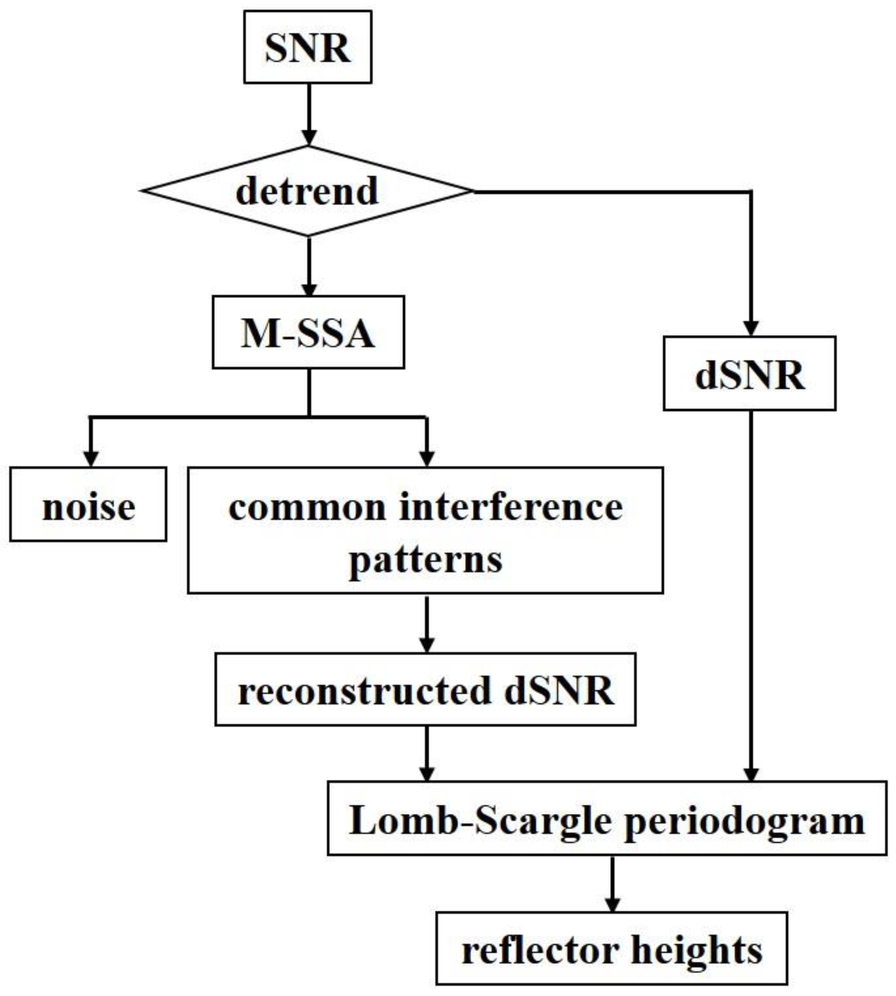
2.2. Mathematical Framework of M-SSA

Multichannel SSA, often referred to as M-SSA, is a generalization of SSA to time series of vectors or maps. This multivariate and nonparametric approach separate the time series into statistically independent components within the augmented vector space of interest, without any a priori hypotheses about their spatiotemporal structure or noise characteristics. These statistically independent components can be classified into trends, periodic oscillations, and noise. It is an important feature of M-SSA that the trends need not be linear and that the oscillations can be amplitude and phase modulated. Consider an L -channel time series X l t : l = 1 , , L ; t = 1 , , N with each channel containing N data points that are at equal intervals n t . The first step is to augment each channel X l t : t = 1 , , N , 1 l L of X with M lagged copies of itself,
X ~ l = X l 1 X l 2 . . X l M X l 2 X l 3 . . X l M + 1 . . . . . X l N 1 . . . X l N 1 X l N X l N + 1 . . X l N , 1 l L
and then forming the full augmented trajectory matrix:
X ~ = X ~ 1 , X ~ 2 , , X ~ L .
Thus, the grand lag-covariance matrix C ~ X is given by [26],
C ~ X = 1 N X ~ t X ~ = C 1,1 C 1,2 . . . C 1 , L C 2,1 C 2,2 . . . . . . . . . . . . . . C l , l . . . . . . . . . . . . C L 1 , L C L , 1 C L , 2 . . C L , L 1 C L , L ,
and the blocks in C ~ X are given by
C l , l = 1 N X ~ l t X ~ l ,
with entries
( C l , l ) j , j = C ~ I J = 1 N t = 1 N X l t + j 1 X l t + j 1 ,
where N = N M + 1 , I = j + M ( l 1 ) , and J = j + M ( j 1 ) .
We used the singular-value decomposition to compute the L M eigenpairs (eigenvectors E k and the corresponding eigenvalues λ k , with 1 k L M ) for the L M × L M matrix C ~ X . Each eigenvector E k is composed of L segments of length M , with its elements denoted by E l k ( j ) . The eigenvectors E k of the grand lag-covariance matrix C ~ X are called the empirical orthogonal functions (EOFs), and the eigenvalues λ k represent the variance captured by the corresponding eigenvectors. The spatiotemporal principal components (PCs) A k can be computed by projecting X ~ onto the EOFs:
A k t = j = 1 M l = 1 L X l t + j 1 E l k j , 1 t N .
and one can recover the kth reconstructed component (RC) at time t for channel l by convolving A k with E k :
R l k t = 1 M t j = L t U t A k t j + 1 E l k j ,
in which the normalization factor M t , the lower and upper bounds of summation, L t and U t , are given by
M t , L t , U t = t , 1 , t , 1 t M 1 M , 1 , M , M t N N t + 1 , t N + M , M , N + 1 t N ,
The original time series of channel l ( X l ) can be recovered by adding up all the RCs ( R l k , 1 k L M ) without any information lost. It is also worth mentioning that the R l k captures the phase of the original X l in a least squares sense, so R l k and X l can be superimposed on the same time scale. This is an advantage of the RCs over the PCs, which have length N M and do not contain direct phase information within the window width M .

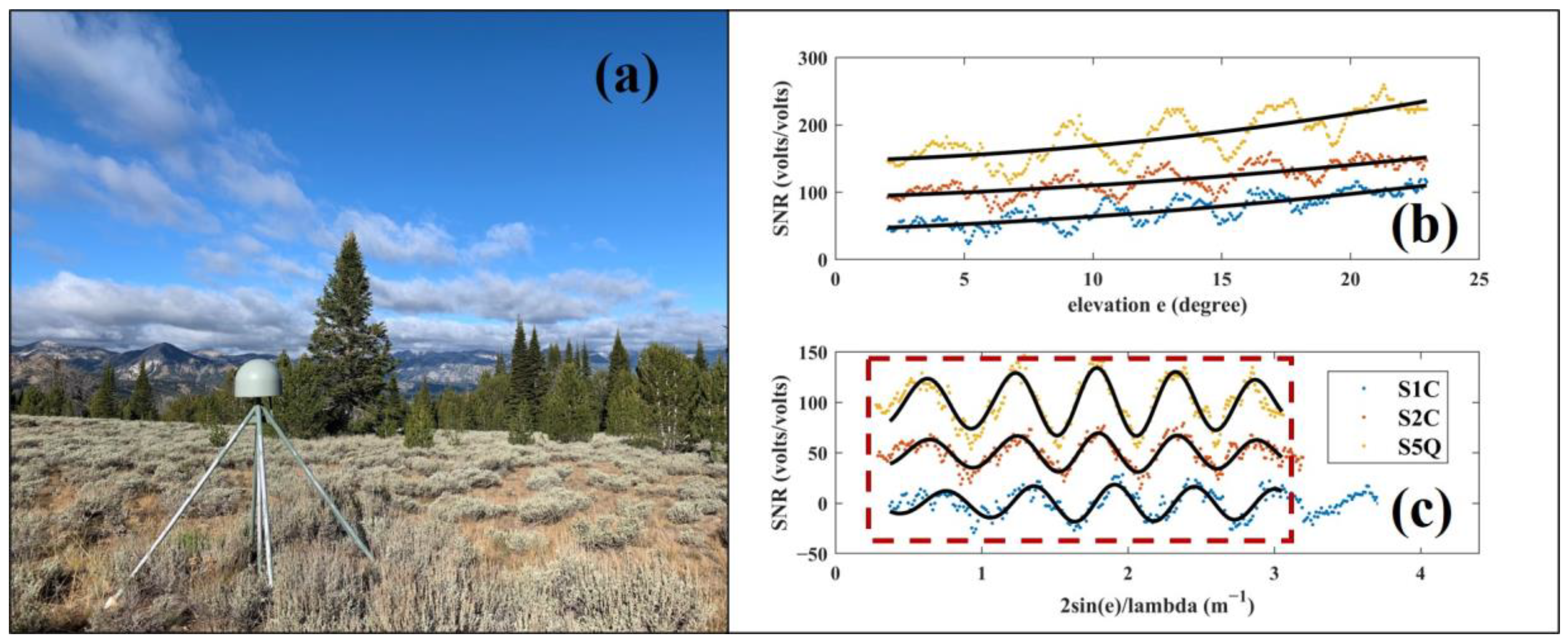
2.3. SNR Measurements

As part of the EarthScope project, the Plate Boundary Observatory (PBO) network consists of over 1200 GNSS and other geodetic instruments located along the western coast of North America [10]. The primary goal of the PBO network is to study plate tectonics, earthquakes, and other geophysical processes. The P351 site of the PBO network is located in Montana Ketchum (~43.87°N, 114.72°W), USA, with an altitude of about 2693 m (Figure 1a). The P351 site records the GNSS measurements, at a sampling interval of 15 s, with a SEPT POLARX5 receiver and a TRM59800 antenna. The P351 is situated in an open environment and experiences approximately 200 days of snow coverage annually, making it a suitable site for GNSS-IR snow depth inversion. The antenna is about 2 m above the gently inclined and undulating ground. The SNR measurements collected at P351 show peaks and troughs as the coherent direct and reflected signals go in and out of phase; these interference fringes are utilized to calculate the reflector height H R based on the inversion model specified in Equation (1) (Figure 1b,c). The L1C, L2W, L2C, and L5Q signals, with their corresponding S1C, S2W, S2C, and S5Q SNR measurements, are recorded and saved in the daily rinex files. Previous studies suggested that, as a result of the semi-codeless method used for tracking the signal that is encrypted by anti-spoofing, or similar techniques, a spurious peak in the LSP may appear for the S2W signal [31]. Therefore, the S2W signal is excluded and SNR measurements of S1C, S2C, and S5Q are used in our experiments. Not all GPS satellites are capable of receiving signals at these three frequencies, and not all setting/rising arcs in every azimuth show significant interference oscillations. SNR measurements from 12 satellites, including PRN01, 03, 04, 06, 08, 10, 18, 24, 25, 26, 30, and 32, were utilized after screening, with a total of 60 days from day of year 250 to 279 in the years 2020 and 2021. The experimental dataset consisting of 840 rising/setting arcs concentrate in a snow-free period and are primarily used (1) to investigate the ability of M-SSA to suppress noise introduced by, e.g., an undulating surface, and (2) to quantify the consistency of reflector heights between different frequencies after M-SSA processing. Although the empirical reflector height of P351 is about 2 m, determining an accurate value is difficult due to its inclined and undulating topography. Therefore, this experiment only provides results of internal consistency (precision) of the inverted reflector heights between different frequencies. By disregarding the subtle differences of the reflection points and of the antenna phase centers among different frequencies, the inverted reflector heights at different frequencies for the same arc, and the same satellite should be theoretically equal or differ by a constant. By comparing and analyzing this kind of consistency for results from (1) the traditional LSP method, (2) SSA + LSP method, and (3) M-SSA + LSP method, the efficiency and advantage of M-SSA in GNSS-IR data preprocessing is demonstrated. The accuracy improvement in the snow height inversion using M-SSA will be discussed in a future study.

3. Results

Figure 2 shows the data processing flowchart of this paper. The original SNR measurements from 840 arcs are first converted from a logarithmic scale in dB-Hz units to a linear scale in Volt units using S N R l i n e a r = 10 S N R / 20 [16], then the detrended SNR (dSNR) time series are isolated by fitting a second-order polynomial (shown as black curves in Figure 1b) to eliminate the low-frequency trends, mainly from direct signals [16]. After conversion and detrending, the resulting dSNR time series in Volt units primarily contain the sinusoidal interference fringes. Next, the sampling independent variable x = e (Figure 1b) is rescaled to x = 2 s i n ( e ) / λ i ( i = 1,2 , 5 ) in order to express the frequencies of the dSNR time series, in terms of the reflector height H R , in meters (Figure 1c). This transformation makes the interference fringes, at different frequencies, dependent only on the reflector height, allowing for the use of M-SSA to extract common oscillations among different frequencies. Although a GNSS receiver tracks signals at even time intervals, the interval between the new axis x during any given observing window will be uneven due to the satellite elevation and its sinusoidal operator. To make the dataset suitable for M-SSA, which requires an evenly spaced input dataset, the dSNR time series are linearly interpolated into equally spaced intervals x = 0.01 , meaning that each unit on the x scale contains 100 samples (Figure 1c). As the lengths of the resampled dSNR time series at different frequencies are no longer equal on the new x axis (a result of the different wavelength λ i for each frequency), and M-SSA requires equal-length input datasets, we chose to use data of the same length ([ 2 s i n ( e m i n ) / λ 1 , 2 s i n ( e m a x ) / λ 5 ]) for the following experiment, as shown by the red box in Figure 1c.
The window size (lag parameter) M of M-SSA plays a crucial role in determining its capability to separate oscillations with similar frequencies. This means that M has to be chosen to ensure that it encompasses at least one complete cycle of the oscillation to be separated. We conservatively selected M = 80 as the window size to separate the periodic oscillation corresponding to an approximate 2-m reflector height. This choice, that 80 intervals are sufficient to encompass one complete cycle of the oscillation, can be justified by observing Figure 1c. After performing M-SSA on the 3-channel dataset in the red box in Figure 1c, we can recover the corresponding reconstructed components (RCs). Figure 3 shows the first 8 RCs corresponding to the first 8 eigenvalues in a decreasing order. Among them, RC1 and RC2 primarily reproduce the oscillations resulting from the interference fringes. Note that the first two EOFs (not shown here), which capture the spatial and temporal variations of the first two RCs, are in quadrature. Such a pair corresponds to the nonlinear counterpart of a sine-cosine pair in standard Fourier analysis for linear problems. The advantage of the EOFs obtained from M-SSA over sines and cosines is that they are not limited to being harmonic functions and can effectively capture anharmonic oscillation shapes. Those amplitude-varying and quasi-sinusoid oscillations often require using multiple harmonics or subharmonics of the fundamental period when performing classical Fourier analysis, whereas a single pair of M-SSA eigenmodes might suffice. This can be confirmed in the RC1–2, where their amplitudes are not constant but change over time. For each frequency, or for each so-called channel, the oscillation amplitudes of the RC1-2 are different. The amplitudes of S1C and S2C are similar and approximately equal to 10 Volts/Volts, while the amplitudes of S5Q are the largest, reaching 20 Volts/Volts, confirming that the L5Q signal has strong effective power and clear fringe visibility. RC3–5 primarily consist of a residual trend, indicating that polynomials are insufficient to fully remove those nonlinear effects from the direct signal. Care should be taken for the impact of the residual nonlinear trend on the inversion of interference fringes when dSNR time series, with low reflector heights, are to be processed. The RC6–8 represent high-frequency noise. According to the model described in Equation (1), only RC1–2, which contain the quasi-periodic signals, are related to the interference oscillations. Therefore, summing up RC1–2 yields filtered versions of the original time series. The black curves in Figure 1c are recovered from RC1–2. The reconstructed dSNR time series effectively captures the interference patterns in the original dSNR time series. For all 840 arcs, the use of only RC1–2 can recover more than 60% of the variance of the original dSNR time series. If the transient trend signals from RC3–5 are added, more than 70% of the variance is recovered. It is worth noting that the previous studies using methods such as empirical mode decomposition, variational mode decomposition, and SSA require the empirical selection of intrinsic modes or singular spectrum components that relate to the interference pattern. By processing multiple dSNR time series at different frequencies simultaneously, M-SSA can effectively recover common-mode interference signals. All RC1–2 reconstructed from our experimental data correctly recover their corresponding interference patterns, indicating that the data-adaptive feature of M-SSA is superior to other univariate methods.
Then, the conventional LSP analysis was applied to the reconstructed dSNR time series to retrieve the reflector height H R . Additionally, the same procedure was applied to the original dSNR time series for comparison. Figure 4 shows results of the LSP analysis of both the original dSNR time series and the reconstructed dSNR time series, where the x-axis represents the estimated reflector height H R and the y-axis represents the linear amplitude in Volts. The results from original dSNR time series show that the value of S1C-inverted H R is 1.70 m, which is approximately 10 cm different from S2C’s 1.78 m and S5Q’s 1.80 m. However, after preprocessing using M-SSA, the estimated H R of S1C, S2C, and S5Q are 1.77 m, 1.78 m, and 1.78 m, respectively, with precision improved to the level of 1 cm. The results indicate that the signal structure, tracking quality, and even wavelength may all have an impact on SNR measurements and the corresponding H R estimates, leading to the poor performance of the legacy L1C signal. The modernized civil signals L2C and L5Q are superior to the legacy L1C signal in the GNSS-IR related studies, since their H R estimates are close to each other even without M-SSA preprocessing. The M-SSA method can effectively extract common modes among signals in different channels and thus, improve the reliability and consistency of estimated H R at different frequencies. Comparing the interference strengths of different frequencies, the L5Q signal shows a stronger amplitude than the S1C and S2C signals, confirming that the L5Q has clearer fringe visibility and better tracking performance than other signals [13]. The amplitude of the reconstructed dSNR time series, using the first two RCs, is higher than that of the original time series, which indicates the capability of noise suppression and information extraction of the M-SSA method.

4. Discussion

The same processing procedure was applied to the original and reconstructed dSNR time series from all 840 arcs to obtain their corresponding H R estimates. Figure 5 compares the consistency between the estimated H R at different frequencies. The top panel, consisting of Figure 5a–c, shows scatter plots obtained using the original dSNR time series, while the bottom panel, consisting of Figure 5d–f, shows scatter plots obtained using the reconstructed dSNR time series. The solid line of linear fitting using the equation y = a x + b between each pair are also given, along with the y = x reference dash line. By disregarding the subtle differences of the reflection points and of the antenna phase centers among different frequencies, the inverted H R at different frequencies for the same satellite and same arc should be theoretically equal or differ by a constant. In our experiment, this means that the closer the coefficient a is to 1, and the closer the coefficient b is to 0, the more consistent the H R estimates are between each two-frequency pair. The consistency between the H R estimates of the S1C signal and those of the S2C and S5Q signals is poor for the original dSNR time series, with coefficient a being 0.77 and 0.76, respectively, and coefficients b reaching 0.49 and 0.51, respectively. Meanwhile, the consistency of the H R estimates between the S2C and S5Q signals is better, with coefficient a being 0.94 and coefficient b being 0.13. The results indicate that, although the L1C signal has the advantage of being tracked for all satellites and always being recorded in the rinex files, the modernized civil L2C and L5Q signals have superior signal quality and better cross-correlation performance. The comparison of results from the original and reconstructed dSNR time series shows a noticeable consistency improvement, in which the values of coefficient a improve from (0.77, 0.76, and 0.94) to (0.97, 0.99, and 1.00), and the values of coefficient b decreased from (0.49, 0.51, and 0.13) to (0.07, 0.03, and −0.01) for S1C–S2C, S1C–S5Q, and S2C–S5Q, respectively. In Table 1, additional statistics of R-squared and RMSE of the linear regression are given. The R-squared are improved from (0.69, 0.67, and 0.89) to (0.95, 0.96, and 0.98), while the RMSE are reduced from (0.10 m, 0.10 m, and 0.06 m) to (0.04 m, 0.04 m, and 0.02 m) for S1C–S2C, S1C–S5Q, and S2C–S5Q, respectively. The consistency between two frequencies is improved by 60%, 60%, and 67%, in terms of the improvement of RMSE. These results again indicate that the signal structure, tracking quality, and even the wavelength of SNR indeed have an impact on SNR measurements and their corresponding H R estimates. By using the M-SSA method, it can effectively extract the common modes in different signals and suppress the impact of noise on the inverted results, thus improving the reliability and consistency of the different-frequency H R estimates. Due to the differences in the H R estimates at different frequencies, it is straightforward to take the average of them as the expectation of H R estimates for the same satellite and the same rising/setting arc. Figure 6 shows the average arc-wise H R estimates for all 840 arcs, along with the corresponding standard deviation 1 σ . Even for a snow-free reflection medium, due to its certain slopes and undulations, the range of H R estimates at different times and different azimuths vary from 1.70 m to 2.30 m, making it challenging to obtain a ‘true’ value to evaluate the accuracy of H R estimates. This is why we only consider consistency and precision but not accuracy. The average of arc-wise standard deviations calculated using the original and reconstructed dataset for all 840 arcs are 4.5 cm and 1.4 cm, respectively. The consistency (or the precision) of the H R estimates between different frequencies has been improved by 69%, which is in line with the improvement of the RMSE mentioned previously. Finally, our results demonstrate good consistency of the L5Q and L2C signals in GNSS-IR reflector height inversion. Benefiting from its faster chipping rate, stronger effective power, and shorter code length, as well as the compatibility and inter-operability among different satellite navigation systems [13], the L5 signal will play a more important role in GNSS-IR related research.
The aforementioned results confirm the potential of M-SSA in improving the consistency of estimating reflector heights at different frequencies, with the input dataset in the form of 3-channel. At the end of this paper, the results of the 2-channel M-SSA and the univariate SSA are presented. Figure 7a–c give scatter plots of the inverted H R from the reconstructed dSNR time series using 2-channel M-SSA, which is composed of S1C–S2C, S1C–S5Q, and S2C–S5Q, respectively. Figure 7d–f are scatter plots between the inverted H R obtained using the univariate SSA individually on S1C, S2C, and S5Q, respectively. Table 1 also summarizes the values of coefficients a and b , as well as R-squared and RMSE of the linear regression. Regardless of whether the original dSNR time series were processed using 2-channel M-SSA or SSA, the consistency between S1C and S2C/S5Q signals is lower than that between S2C and S5Q, which is in agreement with previous results and indicates that the modernized civil signals L2C and L5Q are indeed superior to the legacy L1C signal in GNSS-IR inversion studies. The scatter plots in Figure 7a–c, as well as their fitting lines, are more closely aligned with the reference y = x dash line, since the 2-channel M-SSA method is only composed of dual-frequency data. The values of coefficient a are 1.00, 1.00, and 0.99, respectively, and the values of coefficient b are 0.01, 0.01, and 0.01, respectively. These numeric results suggest that the common inference fringes and corresponding H R estimates extracted by 2-channel M-SSA have better consistency than those obtained by 3-channel M-SSA. However, the R-squared of linear regression using 2-channel M-SSA are 0.88, 0.94, and 0.98, which are slightly lower than the values of the 3-channel case, as well as slightly higher than the RMSE of 0.06 m, 0.04 m, and 0.02 m, respectively. This could be due to the fact that the common oscillation extracted from the 2-channel M-SSA might be overly optimistic. The addition of a more (relatively) independent channel is equivalent to making redundant observations, based on which M-SSA can find the best expectation of the estimates in the least-square way. This so-called data adjustment can lead to a more accurate and reliable result, as errors in individual observations are reduced or eliminated using M-SSA. For the univariate SSA results, the consistency between the inverted H R at different frequencies is lower than the results of 2-channel and 3-channel M-SSA, but better than the results directly obtained using the original dSNR time series. Our experiment demonstrates the ability of the univariate SSA in terms of noise suppression and information extraction. However, it also indicates that the dSNR time series were affected by noise, part of it is closer to Gaussian white noise that can be removed or attenuated by methods such as SSA, while part of it is time-related and may remain in the filtered dataset and impact subsequent inversion results.

5. Conclusions

The data-adaptive and multivariate M-SSA method is effective in separating the time series into long-term trends, periodic oscillations, and high-frequency noise, without relying on a priori hypotheses about their spatiotemporal structure or noise characteristics. In this paper, we applied the M-SSA method to extract common interference patterns from different frequencies simultaneously. The three-frequency (L1C, L2C, and L5Q) SNR measurements from a total of 840 satellite rising and setting arcs, occurring between day of year 250 to 279 in year 2020 and 2021, were used. By comparing GNSS-IR reflector heights obtained from original and M-SSA-reconstructed SNR time series, we found that M-SSA significantly improves the between-frequency consistency, with an increase in the values of R-squared of linear regression from (0.69, 0.67, 0.89) to (0.95, 0.96, 0.98), and a decrease in RMSE from (0.10 m, 0.10 m, 0.06 m) to (0.04 m, 0.04 m, 0.02 m) for S1C–S2C, S1C–S5Q, and S2C–S5Q pair, respectively. The average standard deviation of reflector height estimates at different frequencies for 840 arcs was 4.5 cm for the original dSNR time series and 1.4 cm for the reconstructed dSNR time series. The consistency of reflector height estimates between different frequencies had improved by over 60% in terms of both RMSE and average standard deviation. Our results confirmed the effectiveness of M-SSA in extracting common interference patterns from multi-frequency SNR time series, and demonstrated that the modernized civil signals L2C and L5Q outperform the legacy L1C signal in GNSS-IR studies. Furthermore, the L5 signal’s compatibility and interoperability across different satellite navigation systems makes it a crucial component of future GNSS-IR research.

Author Contributions

Conceptualization, J.L. and S.Z.; Methodology, W.L.; Software, W.L.; Writing—original draft, J.L.; Writing—review & editing, S.Z. All authors have read and agreed to the published version of the manuscript.

Funding

This research was funded by the National Key Research and Development Program of China [2017YFA0603104] and the National Natural Science Foundation of China [42074006].

Data Availability Statement

The GNSS data used in this study are available at: https://data.unavco.org/archive/gnss/rinex/obs/, accessed on 14 February 2023.

Conflicts of Interest

The authors declare no conflict of interest.

References

  1. Nievinski, F.G.; Larson, K.M. An open source GPS multipath simulator in Matlab/Octave. GPS Solut. 2014, 18, 473–481. [Google Scholar] [CrossRef]
  2. Nievinski, F.G.; Larson, K.M. Forward modeling of GPS multipath for near-surface reflectometry and positioning applications. GPS Solut. 2013, 18, 309–322. [Google Scholar] [CrossRef]
  3. Roesler, C.; Larson, K.M. Software tools for GNSS interferometric reflectometry (GNSS-IR). GPS Solut. 2018, 22, 80. [Google Scholar] [CrossRef] [Green Version]
  4. Ran, Q.; Zhang, B.; Yao, Y.; Yan, X.; Li, J. Editing arcs to improve the capacity of GNSS-IR for soil moisture retrieval in undulating terrains. GPS Solut. 2022, 26, 19. [Google Scholar] [CrossRef]
  5. Nievinski, F.G.; Larson, K.M. Inverse Modeling of GPS Multipath for Snow Depth Estimation—Part I: Formulation and Simulations. IEEE Trans. Geosci. Remote Sens. 2014, 52, 6555–6563. [Google Scholar] [CrossRef]
  6. Nievinski, F.G.; Larson, K.M. Inverse Modeling of GPS Multipath for Snow Depth Estimation—Part II: Application and Validation. IEEE Trans. Geosci. Remote Sens. 2014, 52, 6564–6573. [Google Scholar] [CrossRef]
  7. Hu, Y.; Wang, J.; Li, Z.; Peng, J. Ground surface elevation changes over permafrost areas revealed by multiple GNSS interferometric reflectometry. J. Geod. 2022, 96, 56. [Google Scholar] [CrossRef]
  8. Wang, X.; Zhang, Q.; Zhang, S. Sea level estimation from SNR data of geodetic receivers using wavelet analysis. GPS Solut. 2019, 23, 6. [Google Scholar] [CrossRef]
  9. Tabibi, S.; Nievinski, F.G.; van Dam, T.; Monico, J.F.G. Assessment of modernized GPS L5 SNR for ground-based multipath reflectometry applications. Adv. Space Res. 2015, 55, 1104–1116. [Google Scholar] [CrossRef] [Green Version]
  10. Larson, K.M.; Nievinski, F.G. GPS snow sensing: Results from the EarthScope Plate Boundary Observatory. GPS Solut. 2012, 17, 41–52. [Google Scholar] [CrossRef]
  11. Fontana, R.; Latterman, D. GPS Modernization and the Future. In Proceedings of the IAIN World Congress and the 56th Annual Meeting of The Institute of Navigation, San Diego, CA, USA, 28 June 2000. [Google Scholar]
  12. Steigenberger, P.; Thölert, S.; Montenbruck, O. Flex power on GPS Block IIR-M and IIF. GPS Solut. 2019, 23, 8. [Google Scholar] [CrossRef] [Green Version]
  13. Navstar, G.P.S. Space Segment/Navigation User Segment Interfaces. In Interface Specification; (IS-GPS-200E); National Coordination Office for Space-Based Positioning, Navigation, and Timing: Washington, DC, USA, 2013. [Google Scholar]
  14. Wang, X.; He, X.; Zhang, Q. Evaluation and combination of quad-constellation multi-GNSS multipath reflectometry applied to sea level retrieval. Remote Sens. Environ. 2019, 231, 111229. [Google Scholar] [CrossRef]
  15. Strode, P.R.R.; Groves, P.D. GNSS multipath detection using three-frequency signal-to-noise measurements. GPS Solut. 2015, 20, 399–412. [Google Scholar] [CrossRef] [Green Version]
  16. Martín, A.; Luján, R.; Anquela, A.B. Python software tools for GNSS interferometric reflectometry (GNSS-IR). GPS Solut. 2020, 24, 94. [Google Scholar] [CrossRef]
  17. Zhang, S.; Liu, K.; Liu, Q.; Zhang, C.; Zhang, Q.; Nan, Y. Tide variation monitoring based improved GNSS-MR by empirical mode decomposition. Adv. Space Res. 2019, 63, 3333–3345. [Google Scholar] [CrossRef]
  18. Li, Z.; Chen, P.; Zheng, N.; Liu, H. Accuracy analysis of GNSS-IR snow depth inversion algorithms. Adv. Space Res. 2021, 67, 1317–1332. [Google Scholar] [CrossRef]
  19. Hu, Y.; Yuan, X.; Liu, W.; Hu, Q.; Wickert, J.; Jiang, Z. Snow depth estimation from GNSS SNR data using variational mode decomposition. GPS Solut. 2022, 27, 33. [Google Scholar] [CrossRef]
  20. Hu, Y.; Yuan, X.; Liu, W.; Wickert, J.; Jiang, Z. GNSS-R Snow Depth Inversion Based on Variational Mode Decomposition With Multi-GNSS Constellations. IEEE Trans. Geosci. Remote Sens. 2022, 60, 1–12. [Google Scholar] [CrossRef]
  21. Ansari, K.; Seok, H.W.; Jamjareegulgarn, P. Quasi zenith satellite system-reflectometry for sea-level measurement and implication of machine learning methodology. Sci. Rep. 2022, 12, 21445. [Google Scholar] [CrossRef] [PubMed]
  22. Liu, S.; Yue, J.; Chu, Z.; Zhu, S.; Liu, Z.; Wu, J. An improved snow depth retrieval method with adaptive noise reduction for GPS/GLONASS/Galileo/BDS multi-frequency signals. Meas. Sci. Technol. 2022, 33, 085011. [Google Scholar] [CrossRef]
  23. Dettinger, M.D.; Ghil, M.; Strong, C.M.; Weibel, W.; Yiou, P. Software expedites singular-spectrum analysis of noisy time series. EOS Trans. Am. Geophys. Union 2012, 76, 12–21. [Google Scholar] [CrossRef]
  24. Ansari, K.; Panda, S.K.; Jamjareegulgarn, P. Singular spectrum analysis of GPS derived ionospheric TEC variations over Nepal during the low solar activity period. Acta Astronaut. 2020, 169, 216–223. [Google Scholar] [CrossRef]
  25. Dabbakuti, J.K.; Peesapati, R.; Panda, S.K.; Thummala, S. Modeling and analysis of ionospheric TEC variability from GPS–TEC measurements using SSA model during 24th solar cycle. Acta Astronaut. 2021, 178, 24–35. [Google Scholar] [CrossRef]
  26. Ghil, M.; Allen, M.R.; Dettinger, M.D.; Ide, K.; Kondrashov, D.; Mann, M.E.; Robertson, A.W.; Saunders, A.; Tian, Y.; Varadi, F.; et al. Advanced Spectral Methods for Climatic Time Series. Rev. Geophys. 2002, 40, 3-1–3-41. [Google Scholar] [CrossRef] [Green Version]
  27. Groth, A.; Ghil, M. Multivariate singular spectrum analysis and the road to phase synchronization. Phys. Rev. 2011, 84, 036206. [Google Scholar] [CrossRef] [PubMed] [Green Version]
  28. Škare, M.; Porada-Rochoń, M. Multi-channel singular-spectrum analysis of financial cycles in ten developed economies for 1970–2018. J. Bus. Res. 2020, 112, 567–575. [Google Scholar] [CrossRef]
  29. Groth, A.; Ghil, M. Monte Carlo Singular Spectrum Analysis (SSA) Revisited: Detecting Oscillator Clusters in Multivariate Datasets. J. Clim. 2015, 28, 7873–7893. [Google Scholar] [CrossRef] [Green Version]
  30. Walwer, D.; Calais, E.; Ghil, M. Data-adaptive detection of transient deformation in geodetic networks. J. Geophys. Res. Solid Earth 2016, 121, 2129–2152. [Google Scholar] [CrossRef] [Green Version]
  31. Wang, X.; He, X.; Xiao, R.; Song, M.; Jia, D. Millimeter to centimeter scale precision water-level monitoring using GNSS reflectometry: Application to the South-to-North Water Diversion Project, China. Remote Sens. Environ. 2021, 265, 112645. [Google Scholar] [CrossRef]
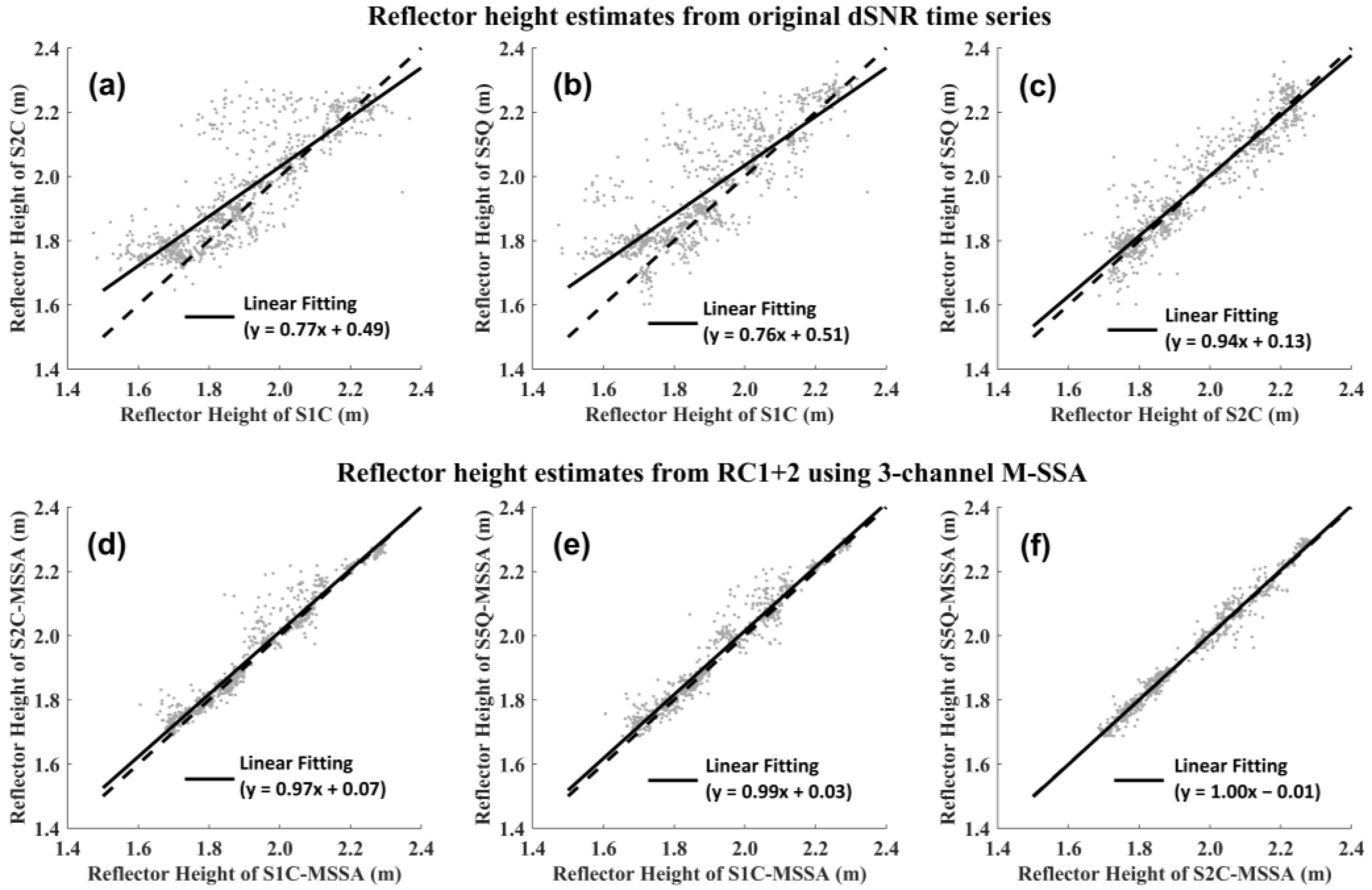
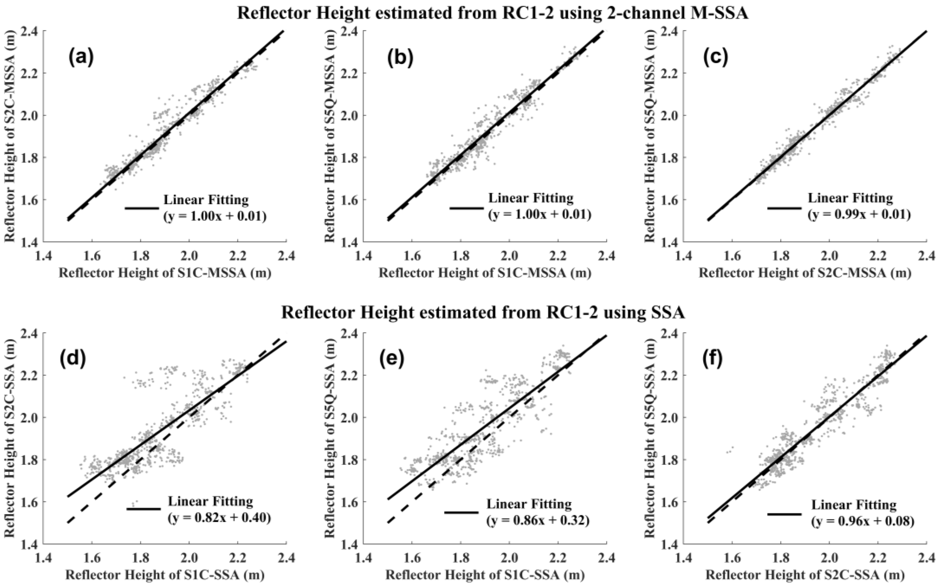
Figure 1. (a) Photograph of P351 GNSS site. The antenna is attached to a ~2-m-height monument. The surrounding environment is open, with a topography gently inclined and undulating. Photo courtesy of UNAVCO. (b) Typical SNR measurements (one rising arc at day 274) as a function of elevation e . All three time-series show interference patterns with low-frequency trends (black curves). Arbitrary constants are added for clarity to the S2C and S5Q signals. (c) The detrended and uniformly interpolated version of (b). A quadratic polynomial is used to remove the direct signal, and a linear interpolation is used to transform the SNR measurements into equally spaced intervals. Note that the x-axis has changed from elevation e to 2 s i n ( e ) / λ . The SNR measurements within the red box are used to form the input dataset for M-SSA. The black curves are the reconstructed time series, by adding the first two reconstructed components, after M-SSA preprocessing. The reconstructed time series effectively recovers the interference patterns in the original time series.
Remotesensing 15 01779 g001
Figure 2. The flowchart of data processing.
Remotesensing 15 01779 g002
Figure 3. The first 8 reconstructed components (RCs) of the dSNR time series of different frequency using M-SSA.
Remotesensing 15 01779 g003
Figure 4. The LSP analysis of the original and reconstructed dSNR time series.
Remotesensing 15 01779 g004
Figure 5. Scatters of estimated reflector heights between S1C, S2C, and S5Q frequencies. (ac) show scatter plots obtained using the original dSNR time series, and (df) show scatter plots obtained using the reconstructed dSNR time series.
Remotesensing 15 01779 g005
Figure 6. The average reflector height in an increasing order and its corresponding standard deviation.
Remotesensing 15 01779 g006
Figure 7. Scatters of estimated reflector heights between S1C, S2C, and S5Q frequencies using 2-channel M-SSA and univariate SSA. (ac) are scatter plots of the inverted H R from the reconstructed dSNR time series using 2-channel M-SSA, which is composed of S1C–S2C, S1C–S5Q, and S2C–S5Q, respectively. (df) are scatter plots between the inverted H R obtained using the univariate SSA individually on S1C, S2C, and S5Q, respectively.
Remotesensing 15 01779 g007
Table 1. Linear fitting statistics between estimated reflector heights from different frequencies using LSP, 3-channel M-SSA + LSP, 2-channel M-SSA + LSP, and SSA + LSP.
Original3-Channel M-SSA2-Channel M-SSASSA
S1–S2S1–S5S2–S5S1–S2S1–S5S2–S5S1–S2S1–S5S2–S5S1–S2S1–S5S2–S5
a0.770.760.940.970.991.011.001.000.990.820.860.96
b0.490.510.130.070.03−0.010.010.010.010.400.320.08
R 2 0.690.670.890.950.960.980.880.940.980.670.730.88
RMSE (m)0.100.100.060.040.040.020.060.040.020.090.090.06
Disclaimer/Publisher’s Note: The statements, opinions and data contained in all publications are solely those of the individual author(s) and contributor(s) and not of MDPI and/or the editor(s). MDPI and/or the editor(s) disclaim responsibility for any injury to people or property resulting from any ideas, methods, instructions or products referred to in the content.

